Article

ADDTID: An Alternative Tool for Studying Earthquake/Tsunami Signatures in the Ionosphere. Case of the 2011 Tohoku Earthquake

by
Heng Yang
1,2,*,
Enrique Monte Moreno
1 and
Manuel Hernández-Pajares
2,3
1
Department of Signal Theory and Communications, TALP, Universitat Politècnica de Catalunya, 08034 Barcelona, Spain
2
Department of Mathematics, IonSAT, Universitat Politècnica de Catalunya, 08034 Barcelona, Spain
3
IEEC-CTE-CRAE, Institut d’Estudis Espacials de Catalunya, 08034 Barcelona, Spain
*
Author to whom correspondence should be addressed.
Remote Sens. 2019, 11(16), 1894; https://doi.org/10.3390/rs11161894
Submission received: 3 July 2019 / Revised: 6 August 2019 / Accepted: 9 August 2019 / Published: 13 August 2019
(This article belongs to the Section Atmospheric Remote Sensing)

Abstract

:
In this work, we characterized the ionospheric disturbances generated during the Japan Tohoku earthquake of 11 March 2011, by means of the Atomic Decomposition Detector of Traveling Ionospheric Disturbances (ADDTID) algorithm. This algorithm automatically detects and characterizes Traveling Ionospheric Disturbances (TIDs) from Global Navigation Satellite System (GNSS) measurements. Applying the high-precision estimates of ADDTID, the propagation parameters would make it easier to distinguish TIDs from different origins, in particular the characteristics conforming the acoustic gravity waves driven by the earthquake/tsunami. This method does not assume that disturbances follow a circular pattern of propagation, and can estimate the location by the propagation pattern of tsunami wavefronts and related TIDs. In this work, we present in a single framework a description of phenomena observed by different researchers. By means of the ADDTID algorithm, we detect: (a) simultaneous TIDs of different characteristics, where the detection was robust against the curvature of the wave fronts of the perturbations and the accuracy of the estimated parameters. The results were double-checked by visual inspection from detrended Vertical Total Electron Content (VTEC) maps and keogram plots, and the parameters of the slow-speed TIDs were consistent with the tsunami waveform measurements; (b) different wavefronts between the west and east TIDs around the epicenter, consistent in time and space with the post-earthquake tsunami; (c) complete evolution of the circular TIDs driven by the tsunami during the GNSS observable area; (d) fast and short circular TIDs related to the acoustic waves of earthquake; (e) the pre-seismic activity consisting of a set of fast westward TIDs, and the comparison with neighboring days; (f) the location estimation of the tsunami wavefront along the coast and the possible use as early warning. Finally, we report disturbances that had not been previously published with a possible application to local and real-time detection of tsunamis.

Graphical Abstract

1. Introduction

In this article, we will analyze the relationship between earthquake/tsunami signatures in the ionosphere, in the form of Traveling Ionospheric Disturbances (TIDs). We will do this using as a tool the Atomic Decomposition Detector of Traveling Ionospheric Disturbances (ADDTID) algorithm developed in Yang et al. [1]. The article contribution is the use of a method for automatically characterizing the earthquake/tsunami interaction with the ionosphere from the GNSS signals. The main advantage of this method is that it does a local (in the geographical sense) estimate of the TIDs parameters such as number of TIDs, and provides a detailed time evolution of the azimuth, wavelength, velocity, and period of each TID. This information is not easy to estimate from the detrended Vertical Total Electron Content (VTEC) maps or from the keograms. One aspect to highlight is that the estimation for detecting the tsunami interaction with the atmosphere is done automatically, without human intervention. In addition, because the estimate is done locally, it generates time series of the parameters of the TIDs. Furthermore, the method can characterize the asymmetries in propagation azimuth, wavelength, amplitude, and velocity. These asymmetries occur in the case of disturbances as in the case of disturbances caused by an earthquake near the coast. The irregular shape of the coast and the different depth of the sea influence the propagation velocity and directions of the waves generated by the tsunami. The ionospheric disturbances generated by the earthquake propagate symmetrically from the epicenter, but the disturbances caused by the tsunami propagate in the sea, with velocities that depend on the depth. In addition these disturbances overlap with the ones induced by the Rayleigh waves of the earthquake. In order to evaluate the performance of the algorithm, we will compare the detrended VTEC maps with the estimates given by the algorithm. An interesting point is that small-amplitude ionospheric effects that had gone unnoticed were detected by the ADDTID algorithm and were checked a posteriori in the detrended VTEC maps.
A further contribution of this work is that the ADDTID algorithm can estimate parameters of simultaneous perturbations in a given region, as was shown in Yang et al. [1] and Yang et al. [2]. This allows a clearer distinguishing of the properties of the overlapping gravity and acoustic waves. The characterization of these waves of different nature was carried out by a preprocessing at two different detrending lags, i.e., 60-s interval of double time difference and 300-s interval of double time difference. In summary, we performed an automatic analysis of the disturbances detected by the ADDTID method. We divided the detected TIDs into three types according to their possible origin and show the time evolution of the propagation parameters along with geographical properties. (see Section 3).
In the context of this work, we can cite as antecedents the following articles. The relationship between tsunamis and ionospheric disturbances was first reported by Hines [3], who suggested that the ionospheric signature could be employed as an early warning of the occurrence of a tsunami. The reason the ionospheric signature indicates the presence of a tsunami is because a tsunami can cause a displacement of the atmosphere on the surface of the sea and then induce atmospheric waves that propagate up to the thermosphere and subsequently generate amplified perturbations in the ionosphere. The physical explanation [3] is that the exponential decrease of density with height causes an exponential amplification of the atmospheric wave by conservation of the kinetic energy. The model proposed by Peltier and Hines [4] shows that the ionospheric signature of gravity waves is detectable in the form of TIDs, which has been confirmed empirically as the TIDs associated with tsunamis, which have been observed and researched for many years. Similarly, a more recent work, Jonah et al. [5] provide gives clear evidence that relates to the origin of the TIDs with the gravity waves.
As an example of this effect, Artru et al. [6], by means of GNSS network, clearly detected the small-scale ionospheric disturbances of gravity waves generated by a tsunami. This tsunami was triggered by the Peru Mw 8.2 earthquake in 2001, and reached Japan 22 h later. These disturbances observed above Japan indicate that the time delay after the earthquake coincides with propagation time of the tsunami. Another case in point is the 2004 Sumatra Mw 9.3 earthquake. This was analyzed by Lee et al. [7], where the authors measured the ionospheric plasma dynamics, in particular the TIDs related to the tsunami, by the combined observations of 430 MHz incoherent scatter radar and GNSS. They suggest that coupling at the tsunami–sea-atmosphere interface launched gravity waves that propagated for great distances beneath the mesopause and conclude that TIDs were induced on a global scale at the wake of tsunami-launched gravity waves. The 2015 Illapel Mw 8.3 earthquake also generated a tsunami. By means of tens of GNSS receivers, Reddy et al. [8] reported the characteristics of ionospheric perturbations induced by shock acoustic waves of the earthquake/tsunami, proving the advantages of GPS observation networks in imaging tsunami-driven ionospheric perturbations.
The analysis that we will carry out in this work refers to the Japan Tohoku tsunami in 2011 that occurred in the Pacific Ocean, giving rise to a maximum height of 40.5 m. It was triggered by an undersea earthquake off the north-east coast of Japan, with a magnitude of 9.1, which occurred at 05:46 UT on 11 March (the 80th day). This tsunami generated ionospheric perturbations that were recorded by more than 1200 GNSS receivers of the Japan GEONET network. Through the use of this high-resolution network, the presence of TIDs was observed in the precedents [9,10,11,12,13] which the following phenomena are reported: (a) TIDs with circular wave fronts, (b) the distinction between different patterns of the atmospheric gravity waves such as the signature of seismic Rayleigh waves and tsunami-driven acoustic gravity waves. By means of a complementary method of measuring the perturbations, Maruyama et al. [14] report similar disturbances of ionosphere by means of the ionosonde stations. Makela et al. [15] present the Japan tsunami signature of airglow located at Hawaii, associated with GPS measurements of the ground-based GPS receivers and the Jason-1 satellite. Komjathy et al. [16] show that the real-time global TEC monitoring network observed the acoustic and gravity waves generated by earthquake/tsunami could give the potential warnings.
Finally, with the ADDTID algorithm, the authors were able to determine tsunami-driven TIDs, see Yang et al. [1]. The multi-TID characterization tool in contrast with other methods that require visual inspection, was able to automatically detect the partial circular fronts of TIDs whose center matched the epicenter of a small-scale earthquake/tsunami in Japan in 2011. The magnitude of the detected earthquake, was less than 5, and its presence was determined by looking at some low magnitude TIDs detected by the ADDTID which followed a circular pattern. Please note that the visual confirmation of the VTEC movies was done after the detection by the algorithm. The pattern had been overlooked due to its low amplitude. The previous works indicate that if we could characterize the TIDs by means of the signal of a GNSS network, we could use these measures as early warnings of tsunamis. The aim of this work is to study and describe by means of ADDTID the behavior of TIDs that appeared during the 2011 Tohoku-Oki tsunami.

2. Data and Methods

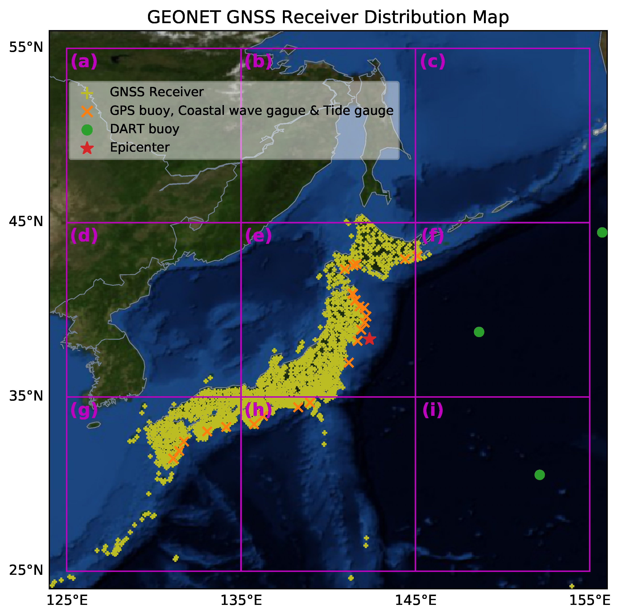
2.1. Source of Data Used and Space Weather

In this study, we use the GPS observation data to detect the ionospheric perturbations. The data come from the GEONET network which consists of about 1200 GPS stations densely distributed in Japan, see Figure 1 [17]. Note in the figure the location of the epicenter, and the partition of the stations in a 10° × 10° grid. This grid will be used for the local estimation of the properties of the TIDs. In addition, we use information from sea measurements to establish the relationship between the pattern of tsunami propagation and measures related to the response of the ionosphere. The data that records the tsunami wave along the coast is provided by the GPS buoys, coastal wave gauges and tide gauges deployed along the Japan coastline [18], and the recording for the tsunami wave in the deep ocean are from DART (i.e., the deep-ocean assessment and reporting of tsunamis) buoys [19], the location is marked with a color code in Figure 1. Note also that in the partitions (g), (h), (f) and (i), these sensors are present, and this will allow us to better contrast the measurements on sea with the measurements from the ionosphere.
The solar and geomagnetic activity measures from [20,21,22,23], indicate that the space weather on the 70th day of 2011 (11 March) was moderate, with no significant disturbances originated by these phenomena such as major solar activity, solar flare, or geomagnetic storm.

2.2. Methodology of GNSS Preprocessing and TIDs Characterization

The process for characterizing of the TIDs associated with the earthquake/tsunami, will be done in two stages.
The first stage consists of the lines of sight computation and GNSS data preprocessing, i.e., obtaining the ionospheric combination from the GNSS carrier phase data, filtering the trend and bias, and mapping the detrended VTEC data, see details in Hernández-Pajares et al. [24]. The technique of detrending employs double difference to eliminate the trends in the ionospheric combinations. The selection of the double difference delays is justified on the basis of the following works: Rolland et al. [10], observed the occurrences of two kinds of TIDs during the earthquake/tsunami, which could be originated from the acoustic waves and atmospheric gravity waves. This was done by means of the band pass filter with the passband of 1–1000 s. They also reported the periods of these two kinds of TIDs centered at the intervals 500–1000 s and about 220–270 s. Galvan et al. [13] also observed the presence of TIDs signatures with a passband of 200–2000 s.
Taking into account the above-mentioned results, in this work we selected both a double difference period of 60 s and one of 300 s. The 300 s interval allows a high sensibility to the tsunami-induced TIDs with the dominant periods in the range of 400–1200 s. The 60 s interval for the double difference is used to filter the trend and preserve the TIDs with the periods centered around the range of 80–240 s. The TIDs in this range are mostly triggered by the Rayleigh waves or/and acoustic resonance after the earthquake.
The hourly hmF2 above the epicenter on this day was from 246 km to 265 km (the climatic hmF2 values are provided by the International Reference Ionosphere 2016 model [25]). In order to better characterize the gravity waves, we assumed that the most frequent dominant TIDs produced by the interaction between the neutral and ion particles occurs below hmF2, see Hernández-Pajares et al. [24], so we took 240 km as the mean effective height of the TIDs, which is lower than the average hmF2. On the other hand, in this same article, experiments are presented in which results are compared at different heights between 100 and 300 km, observing few differences. Thus, the results should be similar to the one reported in Tsugawa et al. [12]. In Appendix B.1, we provide more details about the detection of the ionospheric perturbations by GNSS sounding. We justify the selection of the locations of the Ionospheric Pierce Points (IPPs) at the height of 240 km (Figure A1 left). Also, we show the TEC depletion on slant TECs after the earthquake (Figure A1 right). Furthermore, we present the maps that visually confirm the results of the ADDTID algorithm.
In the second stage, we detect and characterize the parameters of TIDs by means of the ADDTID algorithm. For the mathematical and implementation details, see Appendix A for a summary. In order to characterize the geographical distribution of the detected TIDs, the GEONET GNSS network was divided into nine 10° × 10° mesh subnetworks, and the estimation of the propagation parameters was done for each subnetwork by means of the ADDTID algorithm. The geographical area covered by each subnetwork is marked in magenta in Figure 1 (a)–(i). The ADDTID algorithm can correctly and unbiasedly recover most TIDs and their propagation characteristics even though in some subnetworks (such as (e), (g) and (h)), there is a greater number of IPPs and a better elevation angle. The specific details of the ADDTID implementation adapted to subnetworks are described in Yang et al. [2]. The implementation in subnetworks is justified, because the algorithm locally detects simultaneous plane waves, and the division of the geographic area of study in subnetworks allows approximating arbitrary propagation patterns by means of local planar waves. Please note that in Figure 1, there are regions of the partition without GPS earth stations. The TIDs detected by the algorithm correspond to the IPPs in these regions of satellites with low elevation angle.
An important methodological point is the relationship between the map partition and the position of either the epicenter or the ionocenter. As the TIDs propagate relatively to the ionocenter, we decided to locate the center of the squares (e), (f), (h) and (i), approximately at the ionocenter, so that the disturbances at each element of the grid are as homogeneous as possible. We took as ionocenter, the point mentioned in Tsugawa et al. [12], which is compatible with the propagation of the disturbances shown in Figure A2, where the positions of the epicenter and the ionocenter are marked.

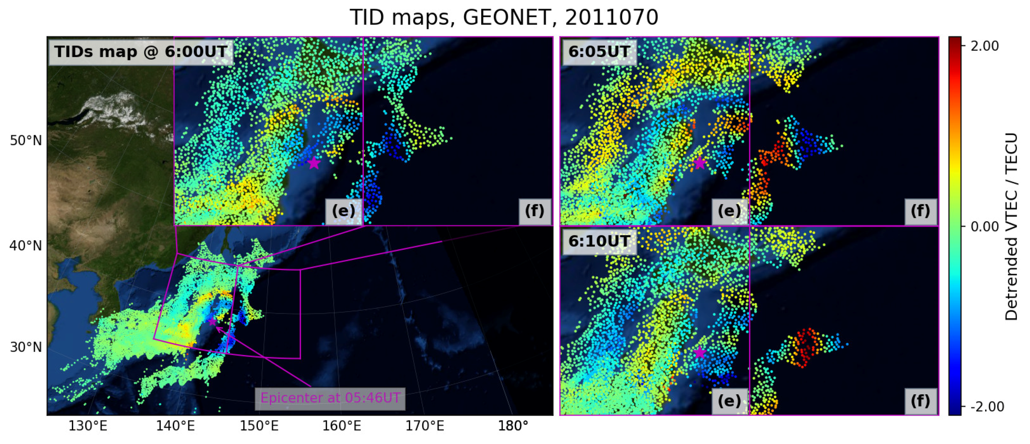
2.3. TIDs Characterization and Description from Detrended VTEC Maps and Keogram Plots

To have a frame of comparison to establish the performance of the ADDTID algorithm, we will present the characterization by visual inspection of detrended VTEC maps and by keograms. The detrended VTEC maps will allow detailed observation of the disturbances, including the fact that some disturbances will appear simultaneously and will be partially superimposed. In the Appendix B.2 we present a detailed analysis of the time evolution of the disturbances, which will allow visual checking of the results of the ADDTID presented in Section 3. In addition, in the Appendix B.3 we present a detailed keogram-based analysis of the disturbances due to the earthquake/tsunami, along with the comparison with the detrended VTEC map time evolution. The keograms are used to represent the evolution in terms of the TIDs, assuming a circular symmetry (i.e., isotropic propagation) to emphasize the features of the response to earthquake/tsunami. In particular, the keograms depict the propagation of the TIDs by means of a plot of the detrended VTECs of the IPPs, organized by the geographical distance from the epicenter. Figure 2 shows two keogram plots, for different detrending periods. To emphasize the different nature of the disturbances related to the phenomenon studied, the left figure plots the keogram for disturbances with the period of 80–240 s and right figure for 400–1200 s. This highlights the presence of ionospheric disturbances with different propagation velocities at different stages of the earthquake/tsunami. In the lower row of the figure we present the state of the detrended VTEC maps at in order to show the physical meaning of the features shown in the keogram, and also to understand the intensity, velocity of the initial high-speed disturbances and asymmetries in the propagation. Please note that to create these keogram plots we used the IPPs set of all the GPS satellites. An interesting fact, is that the keograms shown in the figure, show slopes proportional to the ones obtained by measurements by buoys, as shown in Figure 3, which also hints to the different nature of the disturbances detected, and also, which is important for justifying our findings, the slope, i.e., the speed increases with the depth of the sea.
In the next section, we will discuss the limitations of the above methods, and will show an alternative to the keograms that allow for modelling asymmetries, establishing the geographical location of the each of the specific perturbations, and showing the time evolution of the perturbations by location. Please note that an isotropic assumption is not totally correct, because the disturbances induced by the tsunami [3], will depend on the direction and velocity of the gravity waves from the sea face, which in turn depend on the morphology of the coast and the depth of the sea.

3. Results

In this work we use the ADDTID algorithm to automatically detect and characterize the multi-scale ionospheric disturbances during the period when the Tohoku earthquake and tsunami occurred. We assumed the disturbances to be at a height of 240 km, as is justified in Section 2.2. The estimation of the propagation geometry of the disturbances associated with the earthquake and tsunami is done in nine geographical grids of 10° × 10°. These grids are a partition of the GEONET network located at (25–55°N, 125–155°E), which cover the affected region as shown in Figure 1. We will show the anisotropic propagation of the ionospheric disturbances triggered by the tsunami. In addition, for the time period of 04:00–09:00 UT, we will display the various geographical properties of the perturbations in terms of azimuth, velocity, wavelength, period, and relative intensity. The analysis done by means of the ADDTID consists of the following two items: (a) The description of the disturbances for the duration will be made by means of polar plots and histograms for each element of the grid, i.e., Figure 4 for 04:00–05:45 UT, Figure 5 for 05:45–06:45 UT, Figure 6 for 06:45–07:45 UT, and Figure 7 for 07:45–09:00 UT; (b) The detected disturbances at detrending periods of 60 and 300 s are shown jointly in these diagrams.
As an illustration of how we will carry out the study, we have Figure 4 which shows the analysis for the interval 04:00–05:45 UT. The left polar plots show the azimuth vs. velocity of disturbances at different time intervals of analysis are marked by means of a color code. The diagram is superimposed over each of the nine regions in which we have divided the geographical map. The value of the wavelength is indicated by the radius of the circle located at each detected disturbance (see lateral legend for scale). This makes it possible to clearly distinguish the direction and velocity of the short wavelength perturbations from the long ones. This graphical representation of the multidimensional characteristics of the disturbances enables clear distinguishing of the temporal variation of the disturbances, which is inspired by the visualization of statistical data by Rosling, Hans [26]. In the right subplot of Figure 4, we show the time change of the histograms of the detected propagation parameters. The objective of the histograms is to emphasize the evolution and movement of disturbances in the subnetworks. Please note that in this subplot the color code indicates the cell of the figure to which the histogram corresponds, i.e., represents a given of the azimuth vs. velocity diagram of the left polar plots. This subplot, is complementary in the sense that it allows better distinguishing of the distribution in terms of the detected disturbances. The base scale of the histograms is linear in period, wavelength, and azimuth, but in logarithmic scale for velocity. Finally, the histograms represent a normalized count weighted by amplitudes in logarithmic scale.
In the next two subsections we present the temporal analysis of the geographical distribution of TIDs. Each subsection corresponds to different propagation characteristics related to the earthquake/tsunami, in particular at the pre-seismic stage, the early, middle and final stages of post-seismic period, and each stage is in turn subdivided into smaller time intervals (of the order of 15 min to half an hour) to be able to perform a fine analysis of the events.

3.1. TIDs during the Pre-Seismic Stage

In this subsection we present a summary of the ionospheric state over Japan before the earthquake which spans the period 04:00–05:45 UT (13:30–15:15 LT). The results of applying the ADDTID algorithm are shown in Figure 4.
In the first sub-interval, i.e., 04:00–04:30 UT (red circles in left polar plots) the TIDs appear with an amplitude in the range from 0.08 to 0.2 TEC Unit (TECU, 1 TECU = 10 16 electrons/m 2 ), and most TIDs propagate towards the equator, along with low amplitude and low velocity with westward motions. These TIDs that propagate towards the equator show a wavelength and period in the range of 100–500 km and 10–60 min respectively, which is in agreement with the expected climatology of medium scale TIDs for winter season and daytime [27]. In the right histograms the temporal evolution of TIDs for each sub-interval show a uniform behavior.
The ionospheric disturbances in the next two intervals, i.e., 04:30–05:00 UT and 05:00–05:30 UT (blue and cyan codes in left polar plots), show a significant signature, which are represented by the circles aligned westwards in subnetwork (e), (g), (h) and (f) of left Figure 4. This is also reflected in the histograms, where a clear mode of the azimuth appears at 300 degrees. But most significant feature, is the mode associated with the velocity. The maximum of this mode in the sequence of histograms, shows a linear trajectory in the logarithm scale (base two), i.e., exponential from 300 to 1000 m/s, which correspond to the westward trails that can be also seen in the polar plots. This signature of westward TIDs arises just after 04:00 UT and disappears at about 05:30 UT, with the amplitude of less than 0.1 TECU. This can be appreciated from the beginning as well, but before 04:30 UT is hidden by other detected TIDs with higher intensity and velocity. The histograms show that from the beginning, the signature appears with a low velocity and during the whole duration has a wavelength in the range of 50–120 km.
In the last interval, 05:30–05:45 UT, within 15 min before the earthquake, the TIDs in Figure 4 show low intensities activity and the behavior again corresponds to the climatology. These perturbations, in particular the westwards TIDs, can be appreciated clearly in the movie at [28], but are not detected from the fluctuation of LIs (see Figure A1 right) nor in the keogram plot (see Figure 2). The reason that explains why these TIDs can be observed in the movie but not in the LIs or keograms, is because of the relatively low amplitude in the case of the fluctuations in LIs, and in the case of the keograms plots TEC changes as a function of Euclidean distance, which is not adequate for cases where the predominant waveforms differ significantly from the circular shape.

3.2. Different Speed TIDs after the Main Shock of the Earthquake

At the time of 05:46 UT, the Mw 9.1 earthquake occurred, under the shallow sea of about 32 km depth, located 70 km east of the pacific coast of Japan Tohoku, and the great tsunami with the height up to 40.5 m was triggered in the aftermath [29]. The tsunami waveform recordings from buoys are shown in Figure 3. These recordings were obtained from the GPS buoys, coastal wave gauges, tide gauges, and DART buoys surrounding the epicenter. The recordings show clearly that the triggered tsunami propagates with a low velocity (∼130 m/s) detected by the buoys near the shore, i.e., in shallow sea, and a components of medium velocity (∼230 m/s), detected by the buoys in deep ocean, see similar reports in Fujii et al. [30], Satake et al. [31]. From Figure 3 we measured that the period in the first cycles of the tsunami signal is greater in shallower areas of the sea than in deeper areas. The location of the buoys and the regions of shallow sea can be seen in Figure 1.
Just after the earthquake, for the first ten minutes, the state of the ionosphere is quiet, followed by an outburst of activity, which corresponds to the ionospheric response to the earthquake and subsequent tsunami. The disturbances generated are intense and diverse, reflected as a large-scale temporary depletion of the TEC, followed by long-term fluctuations of the TEC. (see Figure A1 right). In particular, almost circular TIDs are generated, centered approximately in the ionocenter, see the detrended VTEC movies [28]. And also the keogram plot in Figure 2 reveals that these circular TIDs appear with different propagation velocities and have multiply origins, which are compatible with the different tsunami waveforms in Figure 3. Please note that the marked slopes correspond to the arrival of the first wavefront. In the case of the signal from the buoys, aftershocks are more difficult to identify than in the keograms. This behavior of the ionosphere has also been reported in [9,10,11,12]. The time evolution of the decomposition of the global disturbances in its TIDs components, is shown in Figure 5.
To cross-check the results of the algorithm, in Appendix B we present visual summary of the TID behavior during the earthquake/tsunami. At the early stage, the predominant TIDs can be seen visually from the detrended VTEC maps. These make up the concentric circular waves with a horizontal wavelength up to 600 km. These TIDs exhibited the velocity of over 1000 m/s, while another group of TIDs with smaller wavelength subsequently showed much slower velocity. The behavior of the fast ionospheric disturbances probably are launched by the Rayleigh wave or acoustic waves and the dominant ones from the acoustic waves or tsunami, as indicated by Liu et al. [11], Tsugawa et al. [12], Galvan et al. [13]. The disturbances show anisotropic propagation, and several disturbances are superimposed, making it difficult to discern the differences. The TIDs of different nature can be detected either from the two double difference intervals of 60 s and 300 s, or by each separately.
The results of the ADDTID algorithm presented in Figure 5, Figure 6 and Figure 7, show a more nuanced view of the disturbances that appear after the earthquake. The partition of the study region into nine sections makes it possible to study the effects of asymmetry in the propagation of the disturbances, and their different components that could easily go unnoticed. The above-mentioned circular waves can also be appreciated in the map of in Figure 8, which shows a zoom of the regions related to the polar plots (e) and (f) from 06:00–06:10 UT.

3.2.1. Morphology of Fast TIDs Related to Rayleigh Waves

The sudden burst of initial TIDs, could originate from the Rayleigh waves triggered by the earthquake, see Liu et al. [11], Tsugawa et al. [12], Galvan et al. [13]. These Rayleigh waves from the earthquake appear in the keograms of Figure 2, which at about 05:55 UT show disturbances with a high slope (i.e., high velocity). This is also shown in the polar plots and histograms after 05:55 UT in Figure 5, where one can see a high activity of the fast waves in the subnetworks (e), (f), and (h) surrounding the ionocenter. In addition as seen in the histograms of wavelengths, these fast TIDs are associated with wavelengths greater than 500 km. Please note that the ionocenter is located at the southwest of the epicenter. The ADDTID algorithm was designed to detect harmonic shapes (i.e., flat sine waves). Because perturbations appear suddenly (i.e., correspond to a transient), the current implementation detects correctly the direction, wavelength and intensity of propagation correctly, but the variability in the estimation of speed increases when the amplitude decreases, which is the case at hand, because of their low intensity of the initial high-speed TIDs, see Yang et al. [1]. For clarity reasons, in the histograms the upper velocity was limited at 2400 m/s, while in the polar plots, the detected disturbances of higher speed, were represented at the border of the plot. For the sake of clarity, we do not represent off-scale cases in the velocity histogram. Please note that the azimuths of detected TIDs are compatible with those of a circular wave with near the center in the intersection of partitions (e), (f) and (h) as can be seen in Figure 8.
Next we will analyze in more detail how perturbations unfold in time. In Figure 5, a fast large-scale disturbance, with a clear onset and intensity, is detected just before 06:00 UT, and is followed by a series of disturbances at multiple scales and with higher intensities. In subnetworks (e), (f), (h) that surround the ionocenter and (d), the first burst of TIDs appear in the sub-interval 05:45–06:00 UT, propagate in multiple directions, in particular at 70, 250, 300 degrees, i.e., outwards from the ionocenter. The velocity of about 1500–2400 m/s, is compatible with the slope of the first disturbances detected in the keograms. The ADDTID algorithm allows determination that the circular propagation of this first perturbation appears only in the immediate vicinity of the epicenter. Following the first wave, the high-speed disturbances can be clearly distinguished at the histograms of Figure 5.
During the following time interval 06:00–06:45 UT, a set of high velocity perturbations propagating towards the north are briefly detected in subnetworks (b), (e) and (f). Also, in (f), there is a clear component of high-speed disturbances with azimuths in east direction. In addition, southwestward (∼250 degrees), in (e) and (h) disturbances account for most of the high-speed TIDs in this interval. The above-mentioned disturbances show temporal and spatial characteristics of near circular waves propagating outward from the center.
On the other hand, this is a propagation that is clearly asymmetric, since the spread of the velocity varies with the direction. Another asymmetry in the propagation are the TIDs detected at the locations of subnetworks (d) and (g) are farther from the west epicenter than (e) and (h), here the predominant fast disturbances appear with southward propagation (∼185 degrees), and last about 15 min beginning at 06:00 UT. This indicates a clear asymmetric response of different parts of ionosphere with respect to the epicenter, which could be interpreted as the superposition of a near circular disturbance surrounding the epicenter with a southward planar wave in the far west. These TIDs related to the Rayleigh waves are compatible from the ones detected at the keograms, with the aftershocks, in particular the significant ones at 06:08 UT (Mw 6.7), 06:15 UT (Mw 7.9) and 06:25 UT (Mw 7.7) [32]. Also note in the velocity histograms of the subnetworks (d), (e) and (h), with the similar elevation angle for the IPPs, the disturbances in (e) exhibit strongest intensity compared with others (note that the represented histogram is a frequency weighted by amplitude histogram). This intensity distribution of which could be correlated with the distance from in situ to the epicenter. These might indicate that the disturbances related to the Rayleigh waves are attenuated rapidly during the propagation, which can be also observed in the later epochs.
During the later phase, i.e., 06:45–09:00 UT, the fast TIDs diminish and disappear almost in all the subnetworks except (e), with a predominant azimuth of in the range of 240 to 270 degrees, see Figure 6 and Figure 7. Compared with the fast waves in the early moment after earthquake, there are fewer detected disturbances, and their intensity is much weaker. These might be related to the Rayleigh waves produced after the smaller subsequent aftershocks, for instance the ones at 06:59 UT (Mw 6.3), 07:15 UT (Mw 6.3), 07:29 UT (Mw 6.3) and 08:19 UT (Mw 6.5) [32]. Particularly in the polar-plot (e) of Figure 6, there is a set of high-speed perturbations with azimuth about 290 degrees (magenta circles), which is related to the aftershock at 08:19 UT (Mw 6.5). In the histograms related to the velocity, there is a small peak at 08:23 UT with speed of about 1200 m/s that increases to 1800 m/s in an exponential way (note the log scale of the plot). Moreover, the wavelength and period histograms of the fast waves during the whole periods concentrated at about 400–600 km and 100–300 s, respectively, which are consistent with Rolland et al. [10], Galvan et al. [13].

3.2.2. Anisotropic Propagation of Medium- and Slow-Speed TIDs Driven by Tsunami

Next we will describe the medium and low velocity perturbations related to the tsunami. In the early moments after the earthquake, a couple of TIDs with the velocity in the range of 100–300 m/s appear suddenly in the subnetworks close to the epicenter, marked by blue colors in polar plots of Figure 5, in particularly they appear clearly at about 06:10 UT in (e), (f), (h) and (i). The local azimuths in each subnetwork, give tangent planes to a circular wave, that is consistent with the concentric waves observed on the snapshots of detrended VTEC maps in Figure A2 right.
The geographical partition allows us at this spatial scale to approximate the wave locally as a plane wave. The ADDTID algorithm estimates the propagation parameters of most TIDs during 05:45–09:00 UT with wavelengths in the range of 200–400 km and amplitudes in the range of 0.4–1.2 TECU.
Furthermore, a subset of TIDs with larger wavelength of 300–500 km and a faster velocity of about 600–1200 m/s also show almost circular propagation. This has been detected even Figure 5 (f) east from the epicenter, where we had very few valid GNSS observations.
From 06:15 to 06:45 UT, the circular ionospheric disturbances, have reached the subnetworks which are far away from the epicenter, as shown in the subplots of Figure 5 (b), (c), (d) and (g). The histograms of this figure show three types of disturbances with different propagation features in the subnetworks, (1) the predominant TIDs driven by tsunami-induced gravity waves, with the amplitude up to 1.2 TECU, have the medium scale wavelength and velocity of 50–400 m/s, (2) the weakest ones with the amplitude up to 0.15 TECU, related to the acoustic waves originated by the an acoustic wave from the sea surface, have the larger wavelength of 300–500 km and higher velocities in the range of 600–1200 m/s, and (3) with the fastest, the ones induced by the Rayleigh waves. These perturbations have the largest wavelengths, travel at more than 1500 m/s, and show a lower amplitude of about 0.05–0.3 TECU. See detailed discussion see Section 3.2.1. These three patterns of behavior have been reported and discussed in [9,10,11,12,13,33], which can also be double-checked in the keogram plots.
Please note that the TIDs still occur in the subnetworks near the epicenter, which correspond to the continuous outward spreading of the concentric circular TIDs. Despite rough geographical information given by the division into nine subnetworks, the TIDs still indicate the approximate location of their center which is adjacent or in the subnetworks (e), (f), (h) and (i).
Next we will describe the anisotropic propagation of the medium- and slow-speed TIDs. The asymmetry in the propagation is observed in the lower row of Figure 2, where at 06:05 UT the disturbances generated by the earthquake show an elliptical shape for both detrending periods, and a different azimuth for the south-western part of the maps. This elliptical shape is related to the geomorphology of Japan, and has an orientation that is different from the one distortion due to the earth map projection. Please note that this asymmetry cannot be appreciated in the keograms.
In a more detailed way, we describe this asymmetry by means of Figure 5. The first phenomenon might be the presence of two main directions of propagation. The full westward propagation can be observed in the polar plots (d), (e), (g) and (h). In this case, most of the perturbations are located around the angles 200 degrees and 300 degrees. The velocity histograms of the dominant disturbances in (e) that propagate northwestward, show two peaks of slow velocity at 50 m/s and 240–350 m/s after the mainshock. Note the fast one of the two peaks gradually goes down to the similar value of about 75 m/s at about 06:45 UT, this is consistent with the time when the waveform of the tsunami first arrives almost all the coast buoys in (e). As seen in the subnetwork (f) (left polar-plot), which is located over the deep sea, the propagation is consistent with the fact that it is located at the east of the ionocenter, and as can be seen in the azimuth histograms of the TIDs between 5:55 UT and 06:00 UT is distributed in an interval ranging between 10 degrees and 150 degrees, with three distinct directions and after 06:00 UT the TIDs are centered around 20 degrees. The histogram peak of the velocity increases from 150 m/s (5:55 UT) to almost 400 m/s (6:25 UT). This is compatible with the measurements given by the buoys in the deep ocean, in particular the ones located less than 2000 km from the epicenter, see Figure 3 for the speed and Figure 1 for the locations. Please note that interaction between the gravity/acoustic waves created by the tsunami is not linear, thus, increase in the velocity of the TIDs reflects a change in the velocity of the sea waves, but is not strictly proportional as mentioned in Hines [3]. This accounts for the behavior observed in both figures. One of predominant components propagates towards the east (∼90–120 degrees), and the velocity increase is consistent with the increase in the depth of the sea. The tsunami disturbances can be modelled as gravity waves, whose velocity has the following expression v = g h , where h is the depth of the sea (see Freegarde [34], Chap. 4). A similar effect can be seen in subplot (h), where the components on azimuth 170 and 220 degrees show a higher velocity (∼300–450 m/s) than the components (∼100–200 m/s) in the direction to the shore. The subplot (g) also shows a similar behavior, the TIDs that propagate southward propagations, are faster than the ones that propagate westward.
Moreover, another group TIDs in the polar-plot (f) of Figure 5 show a different azimuth, i.e., northeast (∼30 degrees). The histograms associated with this group of TIDs are specific of (f) (marked in green), and from 06:10 UT on show a peak at this azimuth as seen in the azimuth. The velocity diminishes from about 200 m/s and in the stage 06:30–06:45 UT, and exhibits a low velocity of less than 100 m/s, which correspond to disturbances propagating parallel to the junction line of the two plates. These disturbances might be originated from the northeastward propagation of tsunami in the shallow water, assuming that the disturbances at the northeast of the ionocenter were originated from a geographical location near the epicenter. Also, from the histograms one can see that the northeast disturbances (originated from shallow sea) have a much lower intensity than the southwest disturbances (originated from deep ocean). Please note that this relationship velocity/intensity of the disturbance is opposite to the relationship found in other subnetworks. One possible explanation is that the detrended VTEC in this subnetwork is observed from a low elevation angle that would result in and aggravate the non-uniform distortion of intensity.
In the case of the wavelengths of the slow TIDs, just after the earthquake, the spread is high, and almost uniform in all the polar plots of the partition, with a slow increase on the number of TIDs detected in subplot (e), with a spread that decreases and a maximum of the histogram that decreases from 400 km to about 200 km. Please note that the period of the slow TIDs with the velocity lower than 100 m/s have the periods greater than 60 min, while the faster ones have the periods of about 30–60 min. This period distribution is compatible with the detected period of the first cycles after arrival of the tsunami waves from the buoys in shallow sea and deep ocean, see the red lines marked in Figure 3.
In the middle stage, 06:45–07:45 UT, Figure 6 left shows that the circular tsunami-driven TIDs with the wavelength of 200–300 km appear in all subnetworks except the most external (a), (c) and (i). Subnetwork (e), in the interval from 06:45 UT to 06:55 UT, shows a set of disturbances that propagate with an azimuth of 240 degrees, which are common to (d), (g) and (h). The TIDs in (e) continue to show the main peak of the velocity lower than 100 m/s until 07:45 UT, which is consistent with the slopes in the keogram plots. In Section 4.2, we provide more information about the change of velocity at each subplot, and relate it to the propagation of the tsunami. Please note that the activity of the slow TIDs in (e) and (h) begin to exhibit the decreased intensity since 7:00 UT, while the similar attenuation of the TIDs occurs in (d) and (g) with a delay of 65 min.
In the final stage of the analysis, 07:45–09:00 UT, see Figure 7, these TID activity drops gradually. As seen in the polar plots, the azimuth distribution has two modes, one about 310 degrees, and another about 90 degrees, which are the outward propagation of circular disturbances driven by the ripples of the tsunami. At the end of the final period, 08:30–09:00 UT, the TIDs related to tsunami almost disappear and the ones with the small-scale wavelength, related to the ionospheric response to the solar terminator, show the westward propagation similar to the moment before the earthquake (see Section 3.1), distinguishing themselves by having a higher intensity. This shows the tsunami is fading away from this moment on, which is compatible with the detrended VTEC maps and the keogram plots, shown at Figure A2 and Figure 2.

4. Discussion

4.1. Pre-Seismic Westward TIDs

Within about one hour before the main shock, a set of fast small-scale TIDs moving westward, see Section 3.1, show incompatible propagation characteristics compared to the winter daytime behavior [27]. The westward direction is perpendicular to interface of the Pacific Plate is subducting under the plate beneath northern Honshu. Agreeing in time and space, with the findings reported by Heki [35], Kamogawa and Kakinami [36], we find that about 40 min before the earthquake there is a pre-seismic TEC anomaly in the form of the TEC enhancement. This westward moving perturbation in Figure 4, does not have a counterpart in the measurements from the buoys (see Figure 3). Please note that there is a small-scale earthquake Mw 4.2 at 04:12 UT, but the TIDs do not show any special pattern both before and after this earthquake. In order to clarify if the detected fast small-scale TIDs could be the pre-earthquake signals, in Table 1, we summarize the ionospheric activity related to six days around the day of the earthquake in the time interval 04:00–06:00 UT (13:30–15:30 LT), and 364/365 days after. The criterion for selecting these days was that the seismic activity was either low or null, close to the earthquake day or season, and avoided the different effects of the seasonal and diurnal variation of TIDs. In Table 1, we show presence or absence of these disturbances, along with the link to the movies of the detrended VTEC. Also, we provide diverse space weather indicators such as the geomagnetic and solar activities. These statistical results show that the these TIDs with very low intensity might not be related to the earthquake but the seasonal or diurnal characteristics, for instance the TIDs induced by the solar terminator during the spring equinox, see Yang et al. [1], Kotake et al. [37], Otsuka et al. [38]. The low intensities of TIDs compared to the equatorward ones might show the weak effects of the solar terminator. Nevertheless, the explanation of this phenomenon as originated by the solar terminator is unlikely. At this time of the day, the solar terminator is far away, and the examination of the detrended VTEC movies in the days surrounding this earthquake, showed that the TIDs generated by the solar terminator appeared several hours afterwards. Note all these results as the movies can be accessed via the Internet (see details in Table 1). Therefore, the westward set of TIDs that appear 40 min before the earthquake, cannot be taken as pre-seismic indicator, although their origin might be related to a geological origin. Nevertheless, the description in terms of the wavelength, change of velocity and geographic distribution of the TIDs that we report, to the best of our knowledge has not been reported.

4.2. Tracking of Tsunami Waves from the Velocity Signature of TIDs

The objective of this section is to track the signature of the coastal tsunami, by the velocity distribution of the disturbances as shown in Figure 9. For this analysis we assume that the sea waves triggered by the earthquake can be described by the equations of a gravity wave, which have a speed proportional to g h . The interaction of the gravity waves on the sea and the ionospheric disturbances is not straight forward, but as shown in Peltier and Hines [4], the increase/decrease of the speed of the sea waves one has a counterpart not necessary linear in the ionospheric disturbances. In the interval before the earthquake the velocity distribution is irregular. Just after the earthquake in the subplot (f), histogram shows an increase of the velocity associated with the observed modes, which is consistent with the fact that this section of the partition of the map is at the east of the earthquake and therefore the depth of the sea is greater than the other partitions of the figure. In section (e), it corresponds to the region of the epicenter and the closest coastal region. In the interval 6:15 UT to 7:00 UT a stronger intensity of TIDs is observed. This intensity is evident in the amplitude of the histograms in Figure 5 and Figure 9. In addition, the measurements from the buoys in Figure 3 on the left (marked (e)) show that at this time interval the amplitude of the measurements is greater than in the other areas of the partition. A significant aspect of Figure 5 and Figure 9 is that the histograms show two maxima, which are centered around 300 m/s and 75 m/s. The slope observed in the measurements of the buoys (Figure 3) corresponds to approximately 130 m/s, which is roughly the weighted average value between the two maxima. This difference in the velocity distribution modes is related to the fact that when the earthquake occurs at a distance from the coast, the disturbance will propagate through areas of the continental shelf and areas outside of the shelf. In Figure 1 we have depicted the depth of the seabed in blue scale. Given the velocity of propagation of the disturbance in the ocean is proportional to the square root of the depth, there will be two maximum velocities and the smallest of them will correspond to the movement of the tsunami along the coast. Please note that the distribution of the modes of the velocity also reflects the presence of aftershocks.
The same pattern appears with a delay of about 15 min in the subplot (h), which is located south of (e). In both cases the final mode of the velocity histogram is of about 75 m/s. The subplot (g), which is located southward, shows two similar patterns between 06:10 UT and 06:20 UT and between 06:25 UT and 06:45 UT, in which the modes of the velocity histograms show a slowing down of the disturbances. In the interval 06:50 UT to 07:10 UT, we can appreciate how the disturbance induced by the tsunami affects one after another the regions into which the area of study is subdivided. Figure 1 shows that the region (h) is adjacent to the region (e). On the other hand, Figure 9 shows the decreasing velocity pattern of the lower mode of the histograms, both in (e) and (h). The descending pattern begins 15 min in advance in (e) with respect to (h). A similar effect is then observed in (g), which is adjacent to (h), this time with a slightly less than half-hour delay. On the other hand, in the region (f), the perturbations appear with a small delay with respect to (e), and with a speed that increases, due to the fact that in this direction the depth of the sea also increases.
The pattern of histograms shown in the figure reflects the movement of the tsunami along the coastal areas of Japan. A possible application of the ADDTID algorithm would be as a real-time tracking method specific to this area of Japan or in any other risky regions with high density of permanent receivers (e.g., California at USA or Mediterranean coast of European Union). It would serve to monitor the various movements of the tsunami, and thus provide early warning of areas that might be affected. Please note that the speed reported in Figure 3, correspond to the first arrival of the waves at each set of buoys, and in this section is related to the effect on the ionosphere at different moments.

5. Conclusions

In this work we have described by means of the ADDTID algorithm the propagation characteristics of multi-speed ionospheric disturbances on the 70th day of 2011 when the Japan Tohoku earthquake/tsunami occurred. We have compared the performance of the ADDTID with the disturbances estimated by visual inspection from detrended VTEC maps, and from keograms. The method that we propose can automatically track and characterize the time evolution of the set of TIDs associated with the earthquake and tsunami. This tracking is done without assumptions on the possible symmetry of the observations. In contrast, the keogram method assumes that the propagation is isotropic, which in the case of the Tohoku earthquake, due to the shape of the Japanese coast is not a correct assumption. In addition, the method allows the discerning between TIDs of different origins that might be difficult to distinguish in the case of visual inspection of detrended VTEC maps. The difficulties might come from superposition of perturbations that propagate in different directions and have different amplitudes. Also, the method has been able to detect TIDs that did not appear in the keograms, but were confirmed by visual inspection on the detrended VTEC maps. In addition, because the detection is automatic, without human intervention, and has a short delay due to the initial transient of the perturbation, this method might be adapted to specific geographical regions and used as an early warning system for tsunamis.
The detected ionospheric disturbances can be categorized into the following two phases. (1) Before the earthquake, the equatorward propagation of detected TIDs show a behavior that is consistent with the typical characteristics in the daytime of winter season. In addition, a set of small-scale TIDs with rapidly increasing speeds are discovered, which are considered to the climatology rather than pre-seismic signature. (2) After the earthquake, the ionospheric response appears as a set of distinct concentric near circular waves for several hours, due to the perturbation from the Rayleigh waves of the earthquake, the acoustic waves and the gravity waves of the tsunami. Corresponding to these origins, the near circular ionospheric disturbances exhibit three types of patterns in terms of propagation parameters. In particular, we have detected the different velocities between the eastward and westward tsunami-driven TIDs around the epicenter, which are consistent with the different height distribution of the tsunami in shallow sea vs. deep ocean. In addition, the local histograms (weighted by the intensity) of the speed evolution of these TIDs at local regions show a synchronization in time when the main wavefront of the tsunami arrives, which can be used as an ionospheric indicator to track the tsunami waves in real-time.

Author Contributions

Conceptualization, H.Y., E.M.M. and M.H.-P.; Methodology, H.Y., E.M.M. and M.H.-P.; Software, H.Y., E.M.M. and M.H.-P.; Validation, H.Y., E.M.M. and M.H.-P.; Writing—Original Draft Preparation, H.Y. and E.M.M.; Writing—Review & Editing, H.Y., E.M.M. and M.H.-P.; Supervision, E.M.M. and M.H.-P.

Funding

This work has been partially supported by the project TEC2015-69266-P (MINECO/FEDER, UE). Also was partially supported by the 2017 SGR-0851 grant of the Generalitat de Catalunya and by the COSTO ESA-funded project (ESA ITT AO/1-9514/18/NL/IA). This work has been partially supported by the scholarship from China Scholarship Council (CSC) under the grant CSC No. 201508390017.

Acknowledgments

We acknowledge the GNSS data of GEONET are provided by the Geospatial Information Authority of Japan, the data of GPS buoys, coastal wave gauges and tide gauges are provided by the Nationwide Ocean Wave information network of Japan, and the data of DART by National Data Buoy Center of U.S. All the code of this project was done in Python using the machine learning library scikit-learn. The data for this paper are available and they can be requested from any of the authors in particular from Heng Yang ([email protected]) and Enrique Monte Moreno ([email protected]).

Conflicts of Interest

The authors declare no conflict of interest.

Appendix A. Outline of TID Detection Algorithm: ADDTID

The analysis of the data was done by means of the Atomic Decomposition Detector of Traveling Ionospheric Disturbances algorithm (ADDTID, see details in Yang et al. [1]). This algorithm uses data from a dense GNSS receiver network, and can detect and characterize TIDs from the ionospheric piercing points (IPPs). The algorithm creates a dictionary of possible waves that encompass the geographical area under study. The estimation is done using only the IPP samples, and solving a convex optimization problem with a regularization term. This algorithm determines the TIDs as the elements of the dictionary that best approximate the observations at the IPPs. Stating the problem in this way has several advantages, mainly that the number of possible waves to be detected does not have to be stated beforehand. Also, and perhaps the most challenging aspect of the estimation problem, the algorithm can work with non-uniform spatial sampling, including the presence of directions with higher density of sensors, or regions of the network lacking sensors.
In this article, (following the presentation in Yang et al. [1]), we have used a dictionary of plane waves. The model of the waves that gives rise to the elements of the dictionary have the following form,
A x , y , t = A 0 cos k · x , y ω ( t t 0 ) + φ 0
where k is the 2D angular wave number vector, with the module k = 2 π λ ; λ is the wavelength and the normal vector k k = ( cos θ , sin θ ) points in the direction of propagation of the wave. The wave amplitude is A 0 . The terms ω , t 0 and φ 0 are the angular frequency, the starting epoch and initial phase of the TID wave, respectively. The corresponding ith dictionary element T i ( x , y ) at epoch t is defined as follows:
T i x , y = cos 2 π λ i x cos θ i + y sin θ i + φ i
The element T i ( x , y ) of the dictionary is characterized by: λ i wavelength, φ i phase, and θ i wave azimuth. The parameters of each element of the dictionary ( θ , λ , and φ ), are quantized as real numbers, with values restricted to realistic ranges.
The dictionary D is constructed by the concatenation of the set of N elements T i ( x , y ) , reshaped as vectors, giving an array D, defined as D = [ T 1 , T 2 , T 3 , , T N ] . The elements T i ( x , y ) are generated by assigning to the parameters { λ , θ , φ } , all possible feasible values in a quantified range. Each element T i ( x , y ) consists of a grid of P v rows and P h columns, i.e., a uniform sampling of the geographical region of interest. Then, the array is reshaped to a vector T i of dimension P v × P h . Please note that the observations correspond to the IPPs; hence, in the estimation of the vector, α t will be done only with the coordinates ( x , y ) corresponding to measured IPPs. Therefore given a dictionary D, we estimate a set of coefficients at time t, which we denote as α t , such that the observation V, is approximated by the product V D α t . The observation vector V, is defined by the values observed at the IPPs of each satellite. In order not to change the notation, from now on the dictionary matrix D, is defined so that for each element of the dictionary we only extract the components at the observed IPPs.
The parameter vector α t , is estimated by means of a trade-off between a loss function (i.e., how well we approximate the observations by means of the model) and a regularization term (i.e., constraints on the possible solutions). The regularization term is used to guarantee that the solution should be sparse, i.e., only a small set of elements of the dictionary will contribute to the approximation. An estimation technique that allows for the trade-off with a sparse set of coefficients is the LASSO (see for instance Hastie et al. [40]), where the norm on the loss function is 2 , and the norm on the regularization term is 1 . Thus, the optimization problem to be solved is,
α t = arg min α t 1 2 V D α t 2 + ρ α t 1
The parameter ρ controls the level of sparsity of the solution, and is determined automatically from the data, as explained at Yang et al. [1].

Appendix B. Visual Summary of the TID Behavior during the Earthquake/Tsunami

In this section, we will describe the behavior of disturbances during the earthquake by means of detrended VTEC maps and the keogram plots. This section is justified in order to check the results obtained by the algorithm ADDTID in Section 3, and is done (a) visually by the detrended VTEC maps and (b) by the partial information given by the keograms. And also confirm new results obtained by the algorithm ADDTID. These results are visually difficult to appreciate and could go unnoticed, while they can be appreciated clearly in the detrended VTEC movies in the locations indicated by the algorithm.

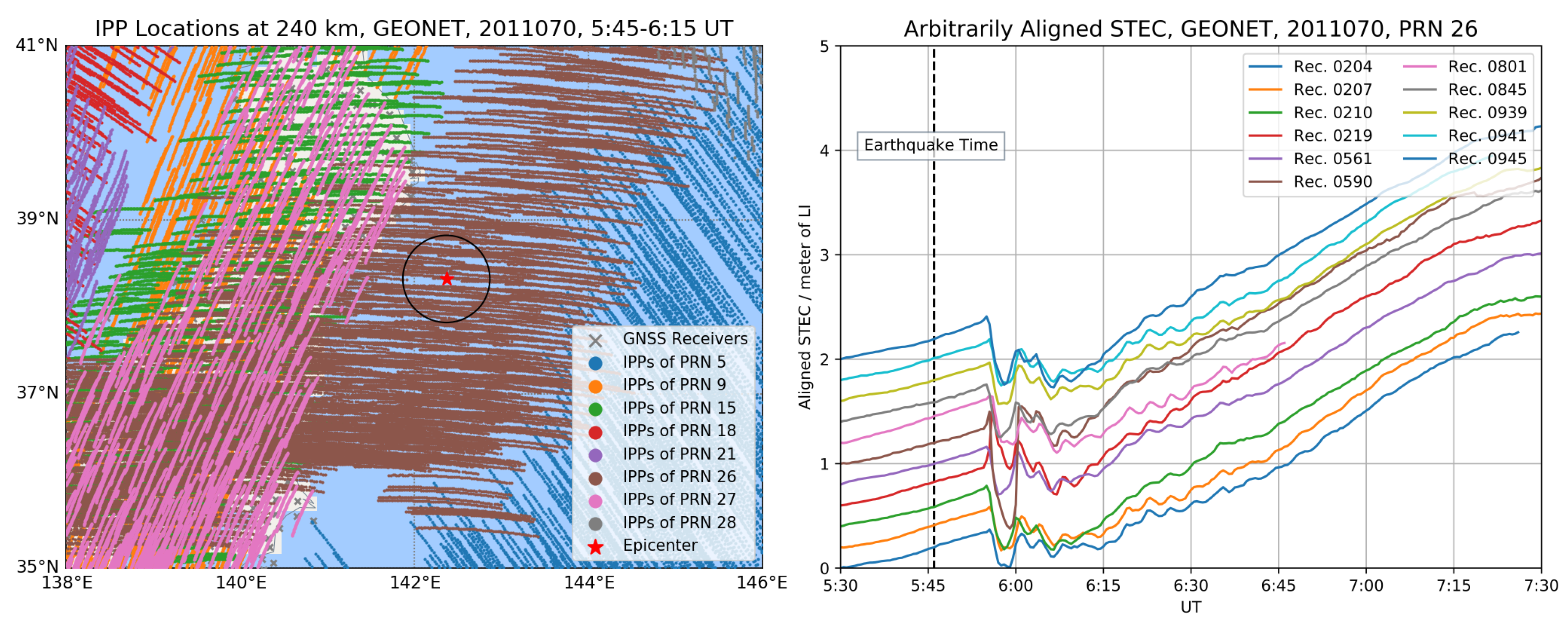
Appendix B.1. Detection of Ionospheric Perturbation by GNSS Sounding

In Section 2.2, we justified the selection of 240 km as the height of the single ionospheric layer during the period of GNSS observation for the earthquake/tsunami event. We show the locations of IPPs at the assumed height in Figure A1 left, from the moment from the time of earthquake to 30 min later. Each color represents for the IPPs set of individual GPS satellite. The locations of epicenter in red star and the IPPs in brown points clearly show that IPPs of GPS satellite PRN 26 record the ionospheric variation information around the epicenter. For this satellite, the observational data of GNSS receivers whose IPP locations are at a distance of less than 250 km from epicenter (marked by the black circle in Figure A1 left) are selected in order to describe the relationship between the ionospheric perturbation and earthquake/tsunami. Also, the receiver observations were filtered out under the losses of lock on GPS. Figure A1 right depicts the slant TECs from these receivers by means of carrier phase ionospheric combination in length units LIs which are arbitrarily aligned to clarify the ionospheric variations. This group of STECs from aligned LIs shows there is a large TEC depletion up to 9 TECUs appeared about 10 min after the earthquake, and drastic ionospheric oscillations after the depletion. Saito et al. [9], Tsugawa et al. [12] also reported similar observations of the sudden decrease of TEC as the response of ionosphere to the earthquake/tsunami.
In the next two subsections, we present the summary of both the detrended VTEC maps and keogram plots.
Figure A1. The left plot: IPP locations at height of 240 km, corresponding to the GEONET GNSS receivers, from 5:45 to 6:15 UT, the color codes of cycles for the IPP locations of different satellites, the grey cross for the location of GNSS receivers, the red star for the location of epicenter; The right plot: Time evolution of the arbitrarily aligned slant TECs, for the GPS satellites PRN 26, at the time of 5:30–7:30 UT, the color codes of lines correspond to different GNSS receivers, the black dash line indicates the time of the earthquake at 5:46 UT.
Remotesensing 11 01894 g0a1

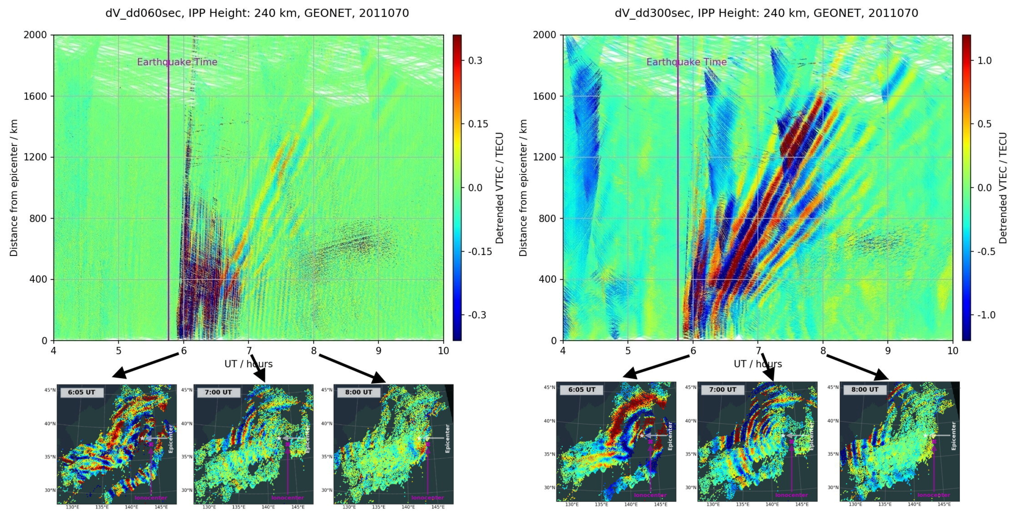
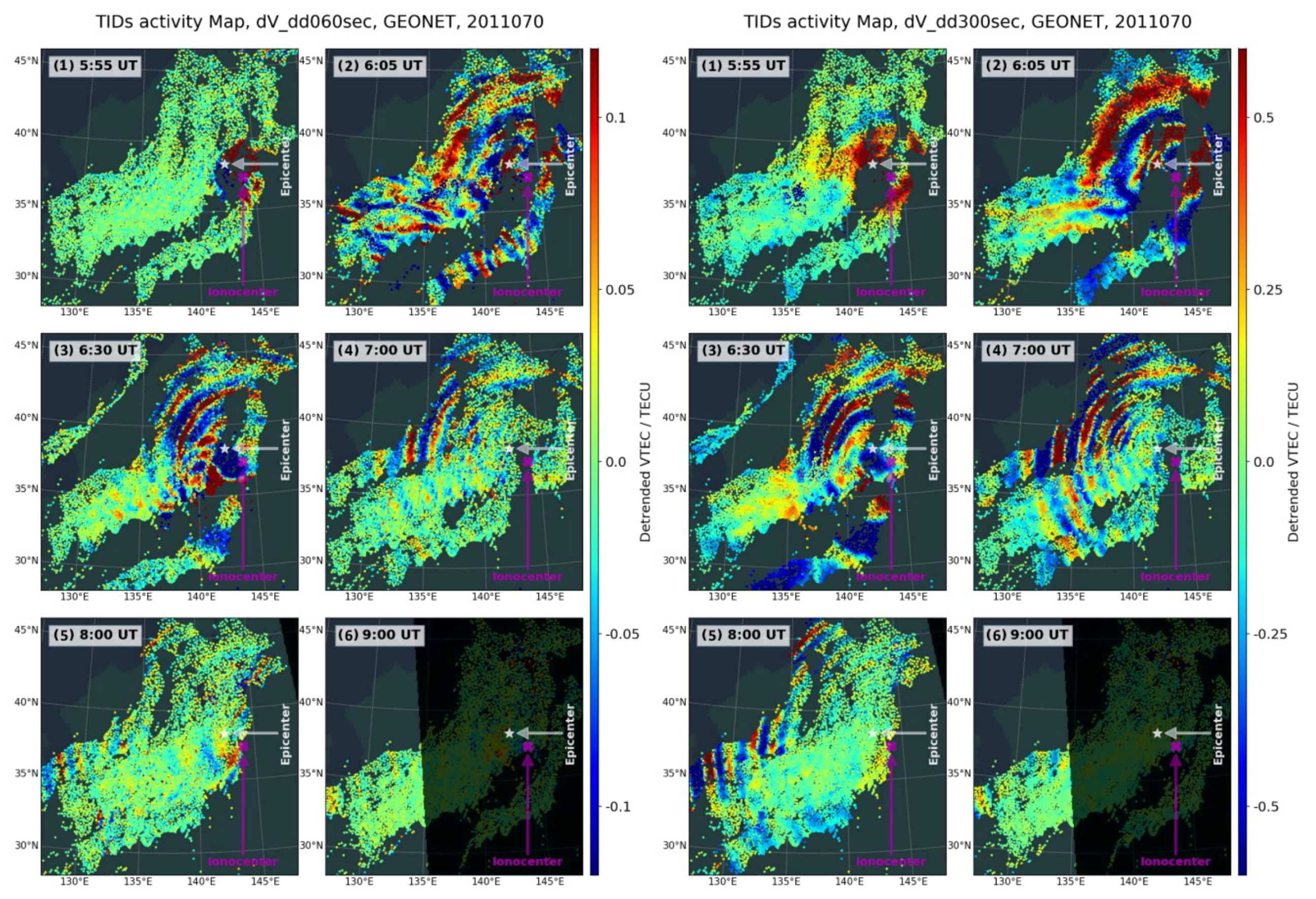
Appendix B.2. TID Propagation Description from Detrended VTEC Maps

To facilitate the tracking of the time and space evolution of the induced ionospheric perturbations, we have organized the TID maps as the movies with the time resolution of 30 s. These two movies can be accessed in the Internet [28].
Next we summarize the time evolution of the perturbations from these two movies by means of a selection of six snapshots taken at relevant moments. The case of 300-s double difference detrending, is shown in Figure A2 right, which depicts six moments of ionospheric fluctuations during the period of earthquake/tsunami from 5:50–9:00 UT. The behavior can be summarized as follows: in the early moment after the earthquake Figure A2 right (1) shows a group of strong ionospheric disturbances suddenly appearing with the time delay of 8–10 min. The following snapshot is was taken 10 min after the first. Figure A2 right (2) shows that the ionosphere exhibits significant disturbances which can be approximated as a circular wave that propagates with large horizontal wavelengths up to 600 km. At 06:30 UT, as shown in the next subplot, the disturbances behave more like the circular traveling disturbances that propagate from the epicenter to the outside. The wavelengths show two different scales respectively located in the inner and outer circles in Figure A2 right (3). After that, the propagation of the smaller scale disturbances follow very clearly a circular wave pattern and until about 09:00 UT, from then on, slowly fading away, see Figure A2 right (4)–(6).
Figure A2. Evolution of TIDs activity maps, detrended by double difference of time interval of 60 s (left plot) and 300 s (right plot), from GEONET network, on the day 70 of 2011, for all the GPS satellites. The maps (1)–(6) are at epochs of 05:55, 06:05, 06:30, 07:00, 08:00 and 09:00 UT respectively.
Remotesensing 11 01894 g0a2

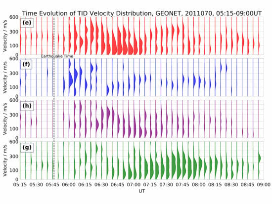
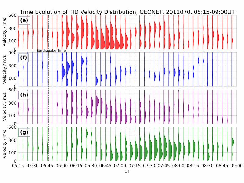
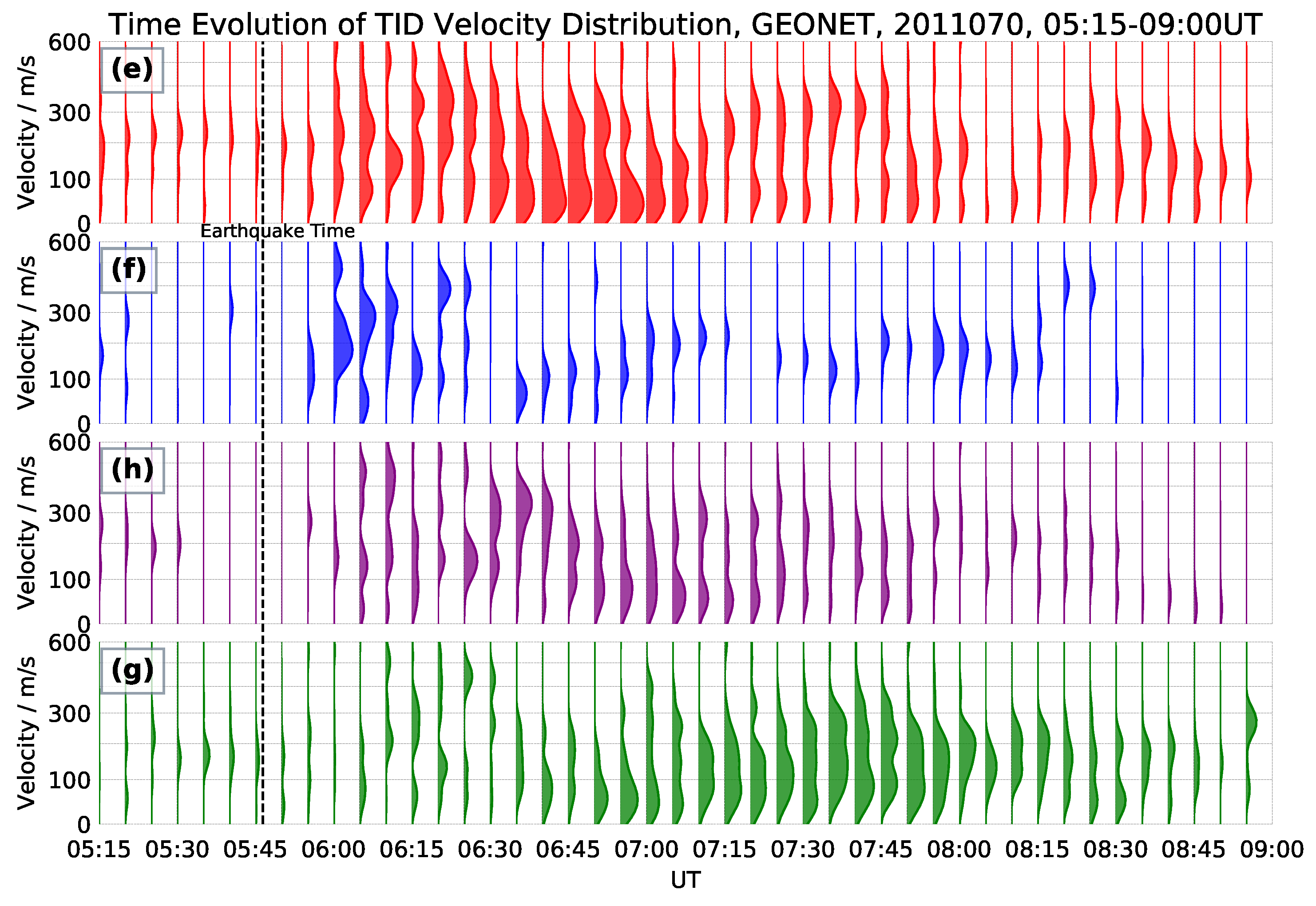
Appendix B.3. TID Characterization and Description from Keogram Plots

For the 60-s double difference detrending case, Figure A2 left shows the same six moments of the detrended VTEC movie, in order to highlight the presence of another group of TIDs. Compared to the disturbances in Figure A2 right, one can discern at least two kinds of the ionospheric disturbances. The TIDs associated with this case show a shorter wavelength, in particular as seen in Figure A2 left (2,3), with a higher velocity, the lower intensity and shorter duration. Please note that the circular TIDs propagate as the concentric waves with centers that does not totally coincide with the epicenter, see the magenta cross symbol in the maps of Figure A2 right.
At the assumed height of 240 km, observe that the center of the circular TIDs is located about 200–300 km southeast of the epicenter. Tsugawa et al. [12] also observe the non-overlapping by assuming the TIDs height of 300 km, and label the center as the ionospheric epicenter. One fact is that the atmospheric waves could be generated by the vertical displacement of the sea surface, the center of TIDs should show the agreement between ionospheric epicenter regarding to the actual epicenter. One possible explanation could be a projection error in assuming the height where TIDs are occurring. Also note some IPPs shows incompatible locations of the wavefronts of the concentric waves, for instance the wavefronts appear in the southwest corner of the epicenter despite different phases, which come from different GPS satellite observation sets, see Figure A2 right (5). This might indicate that the phase of the upward TIDs waves at different heights are measured simultaneously by these GPS satellites, which could be understood as an incomplete tomography scan, while the single layer model of the ionosphere is not enough to analyze the TIDs propagation in this case. Nevertheless, this work only takes into account the horizontal propagation of the TIDs by neglecting the vertical characteristics, and the IPP set of each satellite is independently used to detect TID parameters by ADDTID.
About 10 min after the earthquake, a set of circular disturbances with over 500 km wavelength appear, and initially display very high velocities of about 3000 m/s. In particular, this can be seen in the figure of the detrended VTEC keogram corresponding to the 60-s intervals as shown in Figure 2 (left subplot). These TIDs appearing with the amplitude up to 0.5 TECU is concentrated in the time period of 6:00–7:00 UT and fade away in the next two hours. During this period several aftershocks of the earthquake occur with a lower magnitude, especially during the first hours after the mainshock. Note the propagation radius of the high-speed TID close to the mainshock is more than 2000 km, while the others become shorter over time. This might indicate that both the mainshock and these aftershocks could trigger fast TIDs, the intensity of which is positively correlated with the magnitude of the earthquake. The another set of TIDs with the velocity decreasing from about 3000 down to 750 m/s, display larger wavelengths, see the keogram with 300-s detrending in the right Figure 2.
The third set of TIDs also shows much lower velocities decreasing from 400 to 150 m/s after a short period of time. The circular disturbances can be appreciated clearly in both keograms of Figure A2 right, where the one with 300-s detrending shows higher amplitude. This has also been reported by other authors, for instance in Rolland et al. [10], Liu et al. [11], Tsugawa et al. [12], Galvan et al. [13]. In particular Tsugawa et al. [12], Galvan et al. [13] pointed out the circular TIDs with the velocity of 1000–3000 m/s that are consistent in velocity with the Rayleigh wave. This is one type of surface wave produced during earthquakes, the ones with the velocity of about 750–1000 m/s which should be originated by an acoustic wave generated from the sea surface of tsunami. And the medium scale circular TIDs with lower velocities of 400–150 m/s should be induced by the gravity atmospheric waves from the tsunami.

References

  1. Yang, H.; Monte-Moreno, E.; Hernández-Pajares, M. Multi-TID detection and characterization in a dense Global Navigation Satellite System receiver network. J. Geophys. Res. Space Phys. 2017, 122, 9554–9575. [Google Scholar] [CrossRef]
  2. Yang, H.; Monte Moreno, E.; Hernández-Pajares, M. Detection and Description of the Different Ionospheric Disturbances that Appeared during the Solar Eclipse of 21 August 2017. Remote Sens. 2018, 10, 1710. [Google Scholar] [CrossRef]
  3. Hines, C. Gravity waves in the atmosphere. Nature 1972, 239, 73–78. [Google Scholar] [CrossRef]
  4. Peltier, W.; Hines, C. On the possible detection of tsunamis by a monitoring of the ionosphere. J. Geophys. Res. 1976, 81, 1995–2000. [Google Scholar] [CrossRef]
  5. Jonah, O.; Kherani, E.; De Paula, E. Observation of TEC perturbation associated with medium-scale traveling ionospheric disturbance and possible seeding mechanism of atmospheric gravity wave at a Brazilian sector. J. Geophys. Res. Space Phys. 2016, 121, 2531–2546. [Google Scholar] [CrossRef] [Green Version]
  6. Artru, J.; Ducic, V.; Kanamori, H.; Lognonné, P.; Murakami, M. Ionospheric detection of gravity waves induced by tsunamis. Geophys. J. Int. 2005, 160, 840–848. [Google Scholar] [CrossRef] [Green Version]
  7. Lee, M.C.; Pradipta, R.; Burke, W.J.; Labno, A.; Burton, L.M.; Cohen, J.A.; Dorfman, S.E.; Coster, A.J.; Sulzer, M.P.; Kuo, S.P. Did tsunami-launched gravity waves trigger ionospheric turbulence over Arecibo? J. Geophys. Res. Space Phys. 2008, 113. [Google Scholar] [CrossRef]
  8. Reddy, C.D.; Shrivastava, M.N.; Seemala, G.K.; González, G.; Baez, J.C. Ionospheric Plasma Response to Mw8.3 Chile Illapel Earthquake on September 16, 2015. In The Chile-2015 (Illapel) Earthquake and Tsunami; Braitenberg, C., Rabinovich, A.B., Eds.; Springer: Cham, Switzerland, 2017; pp. 145–155. [Google Scholar] [CrossRef]
  9. Saito, A.; Tsugawa, T.; Otsuka, Y.; Nishioka, M.; Iyemori, T.; Matsumura, M.; Saito, S.; Chen, C.; Goi, Y.; Choosakul, N. Acoustic resonance and plasma depletion detected by GPS total electron content observation after the 2011 off the Pacific coast of Tohoku Earthquake. Earth Planets Space 2011, 63, 863–867. [Google Scholar] [CrossRef] [Green Version]
  10. Rolland, L.M.; Lognonné, P.; Astafyeva, E.; Kherani, E.A.; Kobayashi, N.; Mann, M.; Munekane, H. The resonant response of the ionosphere imaged after the 2011 off the Pacific coast of Tohoku Earthquake. Earth Planets Space 2011, 63, 853–857. [Google Scholar] [CrossRef] [Green Version]
  11. Liu, J.Y.; Chen, C.H.; Lin, C.H.; Tsai, H.F.; Chen, C.H.; Kamogawa, M. Ionospheric disturbances triggered by the 11 March 2011 M9. 0 Tohoku earthquake. J. Geophys. Res. Space Phys. 2011, 116. [Google Scholar] [CrossRef]
  12. Tsugawa, T.; Saito, A.; Otsuka, Y.; Nishioka, M.; Maruyama, T.; Kato, H.; Nagatsuma, T.; Murata, K. Ionospheric disturbances detected by GPS total electron content observation after the 2011 off the Pacific coast of Tohoku Earthquake. Earth Planets Space 2011, 63, 875–879. [Google Scholar] [CrossRef] [Green Version]
  13. Galvan, D.A.; Komjathy, A.; Hickey, M.P.; Stephens, P.; Snively, J.; Tony Song, Y.; Butala, M.D.; Mannucci, A.J. Ionospheric signatures of Tohoku-Oki tsunami of March 11, 2011: Model comparisons near the epicenter. Radio Sci. 2012, 47. [Google Scholar] [CrossRef] [Green Version]
  14. Maruyama, T.; Tsugawa, T.; Kato, H.; Saito, A.; Otsuka, Y.; Nishioka, M. Ionospheric multiple stratifications and irregularities induced by the 2011 off the Pacific coast of Tohoku Earthquake. Earth Planets Space 2011, 63, 869–873. [Google Scholar] [CrossRef] [Green Version]
  15. Makela, J.; Lognonné, P.; Hébert, H.; Gehrels, T.; Rolland, L.; Allgeyer, S.; Kherani, A.; Occhipinti, G.; Astafyeva, E.; Coïsson, P.; et al. Imaging and modeling the ionospheric airglow response over Hawaii to the tsunami generated by the Tohoku earthquake of 11 March 2011. Geophys. Res. Lett. 2011, 38. [Google Scholar] [CrossRef] [Green Version]
  16. Komjathy, A.; Galvan, D.A.; Stephens, P.; Butala, M.; Akopian, V.; Wilson, B.; Verkhoglyadova, O.; Mannucci, A.J.; Hickey, M. Detecting ionospheric TEC perturbations caused by natural hazards using a global network of GPS receivers: The Tohoku case study. Earth Planets Space 2012, 64, 1287–1294. [Google Scholar] [CrossRef] [Green Version]
  17. Sagiya, T. A decade of GEONET: 1994–2003. Earth Planets Space 2004, 56. [Google Scholar] [CrossRef]
  18. Japan MLIT Nationwide Ocean Wave information network for Ports and HArbourS (NOWPHAS). Waveform Measurements of GPS Buoys, Coastal Wave Gauges and Tide Gauges for the Tsunami Triggered by 2011 Mw9.1 Tohoku Earthquake. Available online: https://nowphas.mlit.go.jp/prg/pastdata/static/sub311.htm (accessed on 1 September 2018).
  19. U.S. NOAA National Data Buoy Center (NDBC). Waveform Measurements of DART for the Tsunami Triggered by 2011 Mw9.1 Tohoku Earthquake. Available online: https://www.ndbc.noaa.gov/obs.shtml (accessed on 1 September 2018).
  20. U.S. NOAA National Centers for Environmental Information (NCEI). Solar Data Services: Sun, Solar Activity and Upper Atmosphere Data. Available online: https://www.ngdc.noaa.gov/stp/solar/solardataservices.html (accessed on 7 March 2019).
  21. U.S. NOAA National Centers for Environmental Information (NCEI). Geomagnetic Data. Available online: https://www.ngdc.noaa.gov/geomag/data.shtml (accessed on 7 March 2019).
  22. Japan World Data Center for Geomagnetism. Geomagnetic Equatorial Dst index. Available online: http://wdc.kugi.kyoto-u.ac.jp/dst_final/201103/index.html (accessed on 7 March 2019).
  23. Japan World Data Center for Geomagnetism. Auroral Electrojet Activity Index. Available online: http://wdc.kugi.kyoto-u.ac.jp/ae_provisional/201103/index_20110311.html (accessed on 7 March 2019).
  24. Hernández-Pajares, M.; Juan, J.; Sanz, J. Medium-scale traveling ionospheric disturbances affecting GPS measurements: Spatial and temporal analysis. J. Geophys. Res. Space Phys. 2006, 111. [Google Scholar] [CrossRef]
  25. U.S. NASA’s Community Coordinated Modeling Center. International Reference Ionosphere 2016 Database. Available online: https://ccmc.gsfc.nasa.gov/modelweb/models/iri2016_vitmo.php (accessed on 1 March 2018).
  26. TED Talk: Hans Rosling Shows the Best Stats You’ve Ever Seen. Available online: https://www.ted.com/talks/hans_rosling_shows_the_best_stats_you_ve_ever_seen?language=en#t-265791 (accessed on 1 September 2018).
  27. Hernández-Pajares, M.; Juan, J.; Sanz, J.; Aragón-Àngel, A. Propagation of medium scale traveling ionospheric disturbances at different latitudes and solar cycle conditions. Radio Sci. 2012, 47. [Google Scholar] [CrossRef] [Green Version]
  28. Ionospheric Disturbance Movie over Japan from 04:00-10:00 UT on 11 March 2011. Available online: https://www.youtube.com/playlist?list=PL8I8j8_yCWSYlvUe5sVlQx3Zdm0lqF0FJ (accessed on 5 August 2019).
  29. Mori, N.; Takahashi, T.; Tohoku Earthquake Tsunami Joint Survey Group. Nationwide post event survey and analysis of the 2011 Tohoku earthquake tsunami. Coast. Eng. J. 2012, 54. [Google Scholar] [CrossRef]
  30. Fujii, Y.; Satake, K.; Sakai, S.; Shinohara, M.; Kanazawa, T. Tsunami source of the 2011 off the Pacific coast of Tohoku Earthquake. Earth Planets Space 2011, 63, 812–820. [Google Scholar] [CrossRef]
  31. Satake, K.; Fujii, Y.; Harada, T.; Namegaya, Y. Time and space distribution of coseismic slip of the 2011 Tohoku earthquake as inferred from tsunami waveform data. Bull. Seismol. Soc. Am. 2013, 103, 1473–1492. [Google Scholar] [CrossRef]
  32. U.S. Geological Survey. Earthquake Lists, Maps, and Statistics. Available online: https://earthquake.usgs.gov/earthquakes (accessed on 9 May 2019).
  33. Song, Y.T.; Fukumori, I.; Shum, C.; Yi, Y. Merging tsunamis of the 2011 Tohoku-Oki earthquake detected over the open ocean. Geophys. Res. Lett. 2012, 39. [Google Scholar] [CrossRef] [Green Version]
  34. Freegarde, T. Sinusoidal waveforms. In Introduction to the Physics of Waves; Cambridge University Press: Cambridge, UK, 2012; pp. 47–62. [Google Scholar] [CrossRef]
  35. Heki, K. Ionospheric electron enhancement preceding the 2011 Tohoku-Oki earthquake. Geophys. Res. Lett. 2011, 38. [Google Scholar] [CrossRef] [Green Version]
  36. Kamogawa, M.; Kakinami, Y. Is an ionospheric electron enhancement preceding the 2011 Tohoku-Oki earthquake a precursor? J. Geophys. Res. Space Phys. 2013, 118, 1751–1754. [Google Scholar] [CrossRef]
  37. Kotake, N.; Otsuka, Y.; Ogawa, T.; Tsugawa, T.; Saito, A. Statistical study of medium-scale traveling ionospheric disturbances observed with the GPS networks in Southern California. Earth Planets Space 2007, 59, 95–102. [Google Scholar] [CrossRef] [Green Version]
  38. Otsuka, Y.; Kotake, N.; Shiokawa, K.; Ogawa, T.; Tsugawa, T.; Saito, A. Statistical study of medium-scale traveling ionospheric disturbances observed with a GPS receiver network in Japan. In Aeronomy of the Earth’s Atmosphere and Ionosphere. IAGA Special Sopron Book Series; Abdu, M., Pancheva, D., Eds.; Springer: Dordrecht, The Netherlands, 2011; Volume 2, pp. 291–299. [Google Scholar] [CrossRef]
  39. A Group of Ionospheric Disturbance Movies over Japan from 04:00-10:00 UT on Different Dates. Available online: https://www.youtube.com/playlist?list=PL8I8j8_yCWSZBsbaHxaGvN6mfA82SvyPE (accessed on 5 August 2019).
  40. Hastie, T.; Tibshirani, R.; Wainwright, M. Statistical Learning with Sparsity: The Lasso and Generalizations; CRC Press: New York, NY, USA, 2015. [Google Scholar] [CrossRef]
Figure 1. GNSS receivers and buoys distribution of the GEONET in Japan. Light yellow crosses denote the location of the GNSS receivers, orange X marks denote the location of selected GPS buoys, coastal wave gauges and tide gauges, green circles denote the location of the DART buoys, and the red star denotes the epicenter of the Mw 9.1 earthquake at the time of 5:56 UT, on the 70th day of 2011. The grids in magenta (a)–(i) denote the 9 subnetworks consisting of the geographical grid of 10° × 10°. The ocean depth is shown by the cold color map, originating from the earth observatory of the U.S. NASA blue marble with topography and bathymetry.
Remotesensing 11 01894 g001
Figure 2. Evolution of TID disturbances for the 6 h around the time of the earthquake/tsunami. The TID detrending is done by double differences at time intervals of 60 s (left plot) and 300 s (right plot). The two keogram plots are organized by the geographical distance from the epicenter and the time from 04:00 to 10:00 UT, from GEONET network GNSS data, on the day 70 of 2011, for all the GPS satellites. The lower row aligns the detrended VTEC maps with the keograms to depict their relationship.
Remotesensing 11 01894 g002
Figure 3. Buoys measurements for tsunami waveform during the time interval 05:00–16:00 UT, the left plot denoting the recordings around the Japan Coast, and the right plot for the ones located in deep ocean. The color code of the plots representing the types of recorders: green for the GPS buoys, cyan for the coastal wave gauges, blue for the tide gauges, brown for the DART buoys. The red marks superimposed on the lines denoting the first full cycle of the tsunami after arriving the recorders. The subnetwork labels indicating the geographical locations of the recorders.
Remotesensing 11 01894 g003
Figure 4. Parameter evolution of detected TIDs before the earthquake during 04:00–05:45 UT. Left plots: Non-uniformly scaled polar plots for TIDs of the corresponding grid networks (a)–(i), the location representing for the azimuth vs. velocity of 0–360 degree and 0–2400 m/s, the circle size for wavelength of 50–600 km, and the color code for different time intervals. Right plots: Non-uniformly scaled histograms, weighted by amplitudes, for azimuth, velocity, wavelength, and period, respectively, the color code for TIDs of the corresponding grid networks (a)–(i).
Remotesensing 11 01894 g004
Figure 5. Parameter evolution of detected TIDs after the earthquake during 05:45–06:45 UT. The plot is organized as in Figure 4.
Remotesensing 11 01894 g005
Figure 6. Parameter evolution of detected TIDs after the earthquake during 06:45–07:45 UT. The plot is organized as in Figure 4.
Remotesensing 11 01894 g006
Figure 7. Parameter evolution of detected TIDs after the earthquake during 07:45–09:00 UT. The plot is organized as in Figure 4.
Remotesensing 11 01894 g007
Figure 8. Detrended VTEC maps, at subnetworks (e) and (f), detrended by double difference of 300 s, from GEONET network, on the day 70 of 2011, for all the GPS satellites, at 06:00, 06:05, and 06:10 UT respectively. The ocean depth, obtained from the earth observatory of the U.S. NASA blue marble with topography and bathymetry.
Remotesensing 11 01894 g008
Figure 9. Time evolution of TID velocity distribution during 05:15–09:00 UT, for the subnetwork (e), (f), (h) and (g) respectively. The scale of the velocity axis ranges from 0 m/s to 600 m/s.
Remotesensing 11 01894 g009
Table 1. Statistics of westward ionospheric disturbances during 04:00–06:00 UT, in the selected days of 2011 and 2012.
DateOffset DaysWestward Disturbances Activity [39]Earthquake Event Num.; Max Mag. [32]Planetary K Index (Kp) [21]Solar 10.7 cm Radio Flux (F 10.7 ) [20]Solar Flare X-Ray Class-Num. [20]
1 March 2011−10Not foundNot reported2+111C-7
5 March 2011−6FoundNot reported2+135C-15
9 March 2011−2Found11; M5.61−143C-9; M-2; X-1
11 March 20110Found7; M9.15+123C-12
16 March 20115Not found8; M5.4095C-3
21 March 201110Found4; M5.01−101C-3
9 March 2012364Found1; M4.96+146C-10; M-1
10 March 2012365FoundNot reported5−149C-9; M-1

