A Simplified and Robust Surface Reflectance Estimation Method (SREM) for Use over Diverse Land Surfaces Using Multi-Sensor Data

Abstract

Surface reflectance (SR) estimation is the most critical preprocessing step for deriving geophysical parameters in multi-sensor remote sensing. Most state-of-the-art SR estimation methods, such as the vector version of the Second Simulation of the Satellite Signal in the Solar Spectrum (6SV) radiative transfer (RT) model, depend on accurate information on aerosol and atmospheric gases. In this study, a Simplified and Robust Surface Reflectance Estimation Method (SREM) based on the equations from 6SV RT model, without integrating information of aerosol particles and atmospheric gasses, is proposed and tested using Landsat 5 Thematic Mapper (TM), Landsat 7 Enhanced Thematic Mapper plus (ETM+), and Landsat 8 Operational Land Imager (OLI) data from 2000 to 2018. For evaluation purposes, (i) the SREM SR retrievals are validated against in situ SR measurements collected by Analytical Spectral Devices (ASD) from the South Dakota State University (SDSU) site, USA; (ii) cross-comparison between the SREM and Landsat spectral SR products, i.e., Landsat Ecosystem Disturbance Adaptive Processing System (LEDAPS) and Landsat 8 Surface Reflectance Code (LaSRC), are conducted over 11 urban (2013–2018), 13 vegetated (2013–2018), and 11 desert/arid (2000 to 2018) sites located over different climatic zones at a global scale; (iii) the performance of the SREM spectral SR retrievals for low to high aerosol loadings is evaluated; (iv) spatio-temporal cross-comparison is conducted for six Landsat paths/rows located in Asia, Africa, Europe, and the United States of America from 2013 to 2018 to consider a large variety of land surfaces and atmospheric conditions; (v) cross-comparison is also performed for the Normalized Difference Vegetation Index (NDVI), the Enhanced Vegetation Index (EVI), and the Soil Adjusted Vegetation Index (SAVI) calculated from both the SREM and Landsat SR data; (vi) the SREM is also applied to the Sentinel-2A and Moderate Resolution Imaging Spectrometer (MODIS) data to explore its applicability; and (vii) errors in the SR retrievals are reported using the mean bias error (MBE), root mean squared deviation (RMSD), and mean systematic error (MSE). Results depict significant and strong positive Pearson’s correlation (r), small MBE, RMSD, and MSE for each spectral band against in situ ASD data and Landsat (LEDAPS and LaSRC) SR products. Consistency in SREM performance against Sentinel-2A (r = 0.994, MBE = −0.009, and RMSD = 0.014) and MODIS (r = 0.925, MBE = 0.007, and RMSD = 0.014) data suggests that SREM can be applied to other multispectral satellites data. Overall, the findings demonstrate the potential and promise of SREM for use over diverse surfaces and under varying atmospheric conditions using multi-sensor data on a global scale.

1. Introduction

Due to the cost effectiveness and ready availability of data, satellite remote sensing is now extensively used for deriving various geophysical parameters at a global scale; but, it mostly depends on accurate retrievals of the surface reflectance (SR), i.e., “the fraction of incoming sunlight that the surface reflects”, from the remotely sensed data. SR is thus the most basic remotely sensed parameter in the solar reflective spectral bands (visible and infrared) that is used as an essential input parameter to obtain many parameters including vegetation indices [1], leaf area index [2], burned area identification [3], land cover classification [4], aerosol optical depth [5,6,7], and water quality parameters [8]. It is estimated from the reflectance received by satellites at top of the atmosphere (TOA). However, TOA reflectance is affected by atmospheric constituents that introduce nonnegligible offset and uncertainty in the satellite data. Therefore, before performing any qualitative or quantitative analysis, it is critical to eliminate atmospheric contributions and accurately estimate the SR of a ground target.

Normally, the elimination of the atmospheric contributions and estimation of SR are performed using image-based and physical methods. Image-based methods such as, dark object subtraction (DOS) [9], the empirical line method (ELM) [10], and histogram matching [11] do not employ any physical parameters, e.g., atmospheric direct and diffuse transmissions, water vapor, and ozone, etc., to estimate SR, as they obtain the required ancillary information (solar and sensor viewing geometry) from the image metadata [12]. The most common physical methods are the Atmospheric Correction (ATCOR) [11], the Fast Line-of-sight Atmospheric Analysis of Spectral Hypercubes (FLAASH) [13], the Image Correction (iCOR, previously known as OPERA) [14], the Framework for Operational Radiometric Correction for Environmental monitoring (FORCE) [15], the Landsat Ecosystem Disturbance Adaptive Processing System (LEDAPS) [16], and the Landsat Surface Reflectance Code (LaSRC) [17]. All of these methods estimate surface reflectance based on physical parameters and precalculated comprehensive lookup tables (LUT) which are constructed by radiative transfer (RT) models [18,19,20,21]. The ATCOR, FLASH, and iCOR use the Moderate-resolution Atmospheric Transmission (MODTRAN) RT model [18], FORCE is based on the Simulation of Satellite Signal in the Solar Spectrum (5S) [19], and the LEDAPS and LaSRC applies the vector version of the Second Simulation of the Satellite Signal in the Solar Spectrum (6SV) [20,21] to simulate atmospheric conditions. Such methods are complex in nature compared to image-based methods due to the requirement of several ancillary parameters to simulate atmospheric conditions and correct the data degraded by atmospheric constituents. For example, the 6SV, the most commonly used method in the remote sensing community to eliminate atmospheric contributions and estimate accurate surface reflectance, requires information on vertical profiles of air pressure, water vapor concentration, air temperature, ozone concentration, a digital elevation model (DEM), aerosol optical depth, and an aerosol model as well as the solar and sensor viewing geometry to simulate atmospheric conditions and construct the LUT. The attributed accuracy of 6S, of within 1% [22] is nevertheless subject to inherited errors from the ancillary input parameters [12,23], which are obtained from different sources.

Previous studies have evaluated the various atmospheric correction methods over different types of land covers, atmospheric conditions, and geographical locations [12,24,25,26,27]. For example, Nazeer et al. (2014) [12] validated the SR from both image-based (DOS and ELM) and physical methods (ATCOR, FLAASH, and 6S) over sand, artificial turf, grass, and water surfaces using in situ measured SR, and found the 6S to be robust and more accurate for SR estimation compared to the other methods. Nguyen et al. (2015) [24] tested the adequacy of the DOS, FLAASH, and 6S for above-ground biomass (AGB) estimations of the Gongju and Sejong regions of South Korea and found that 6S outperforms the other methods. López-Serrano et al. (2016) [25] compared the ATCOR, COST (cosine of the Sun zenith angle), FLAASH, and 6S for estimating AGB in the temperate forest area of northeast Durango, Mexico, and concluded that the 6S method is more efficient and reliable than other methods. These validation exercises suggested that (i) the physical methods performed much better than the image-based methods, and (ii) the 6S is the most reliable physical method.

To date, operational SR satellite products are available from the Moderate Resolution Imaging Spectroradiometer (MODIS) [28], the Visible Infrared Imaging Radiometer Suite (VIIRS) [29], the Landsat 4–7 Thematic Mappers (TM) and Enhanced Thematic Mapper Plus (ETM+) (LEDAPS) [16], the Landsat 8 Operational Land Imager (OLI, LaSRC) [17], and the Sentinel-2 A/B Multispectral Instruments (MSI) [30]. In addition to the operational SR products from the Landsat 8 OLI and Sentinel-2 MSI sensors, a Harmonized Landsat and Sentinel (HLS) SR product is generated to improve the global coverage for every 2 to 3 days at a spatial resolution <30 m [31]. A number of efforts have also been made to validate the LEDAPS, LaSRC, and S2 MSI SR products under different conditions and reference data sets [12,17,32,33,34,35,36,37,38].

As evident from all these publications, an accurate estimation of SR based on RT models requires precise retrieval of AOD and vice versa. In other words, these two parameters, i.e., SR and AOD, complement and depend on each other for their inversions. The available state-of-the-art SR methods based on the RT algorithms do not provide a meaningful solution without incorporating information on aerosol particles and atmospheric gases which is a daunting task given the inherent errors in satellite AOD retrievals, which vary spatially and seasonally across the globe [39,40]. Therefore, the prime intent of this study is to provide a user-friendly SR method, which can easily be applied. This study proposes a new Simplified and Robust Surface Reflectance Estimation Method (SREM) based on the equations of the 6SV RT model that can perform SR inversion without using precalculated comprehensive LUT, and information on aerosol particles and atmospheric gases and furnishes results similar to well-known state-of-the-art methods. The outline of the manuscript is as follow: Section 2 is related to the datasets and selection of the validation sites, Section 3 is based on the research methodology for SREM and evaluation process, results and discussions are described in Section 4, and conclusions of this study are summarized in Section 5.

2. Datasets

In this study, archived datasets are used from the satellite sensors, i.e., Landsat 5 (L5) TM, Landsat 7 (L7) ETM+, and Landsat 8 (L8) OLI, for the development of SREM. For validation purposes, in situ SR data from South Dakota State University (SDSU: grassland site) in South Dakota (Figure 1) are taken by Maiersperger et al. (2013) [35]. For comparison purposes, LEDAPS and LaSRC SR products are obtained for 11 urban, 13 vegetated, and 11 desert (arid) sites (Figure 1) from January 2000 to October 2018.

2.1. Satellite Data

Landsat TM/ETM+/OLI

The Landsat TM, ETM+, and OLI sensors were launched in March 1984, April 1999, and February 2013, respectively. Landsat ETM+ scenes acquired since May 30, 2003, have data gaps due to the Scan Line Corrector (SLC) failure and the scenes acquired before this date are defined as non-SLC. All sensors have a spatial resolution of 30 m for the multispectral bands and a revisit time of 16 days. In this study, Landsat TM, ETM+, and OLI data for the visible to near-infrared bands (

Table 1. Spectral bands, band numbers, and central wavelengths (nm) of the L8, L7, and L5 data used in this study.

Spectral Band	Band Numbers
	L8 OLI	L7 ETM+	L4/5 TM
Coastal Aerosol	B1 [443.0]	−	−
Blue	B2 [482.0]	B1 [485.0]	B1 [485.0]
Green	B3 [561.5]	B2 [560.0]	B2 [560.0]
RED	B4 [654.5]	B3 [660.0]	B3 [660.0]
NIR	B5 [865.0]	B4 [835.0]	B4 [830.0]
SWIR1	B6 [1608.5]	B5 [1650.0]	B5 [1650.0]
SWIR2	B7 [2200.5]	B7 [2220.0]	B7 [2215.0]

) are used in the SR retrieval by applying SREM. The new SR data set is compared against the readily available SR products (i.e., LEDAPS and LaSRC) from the respective sensors.

The LEDAPS algorithm is applied to process the L5 TM and L7 ETM+ Level-1 products to SR (Level-2), where the SR is derived automatically from the calibrated TOA reflectance using the 6S atmospheric correction method and atmospheric parameters [16], similar to the MODIS SR products (i.e., MOD09 for Terra and MYD09 for Aqua sensors). In contrast to the LEDAPS algorithm, the LaSRC SR product [17] for the L8 OLI sensor includes improved estimation of the atmospheric parameters (pressure, water vapor, air temperature, ozone, and AOD) essential as input to the RT-model-based SR estimation. The atmospheric parameters for the LaSRC and LEDAPS are obtained from the MODIS Climate Modeling Gridded (CMG) data products and National Centers for Environmental Prediction (NCEP) gridded products, respectively, both based on the 6SV RT model.

For this study, the Collection-1 Landsat data are taken from the United States Geological Survey (USGS), Earth Resources Observation and Science (EROS), Center’s Science Processing Architecture (ESPA) on-demand interface (https://espa.cr.usgs.gov) as Level-1 and Level-2 products for the period of January 2000 to October 2018.

2.2. In Situ Surface Reflectance Data

The ground-truth SR data were collected by Maiersperger et al. [35] from the South Dakota State University’s (SDSU) grassland site in South Dakota (Figure 1) using the Analytical Spectral Devices (ASD) FieldSpec spectrometer. Generally, this site is used by the Committee on Earth Observation Satellites (CEOS) as a reference site for vicarious calibrations. For this site, a total of 10 L5 and L7 scenes were found coincident with the ASD data (Appendix A) for validation.

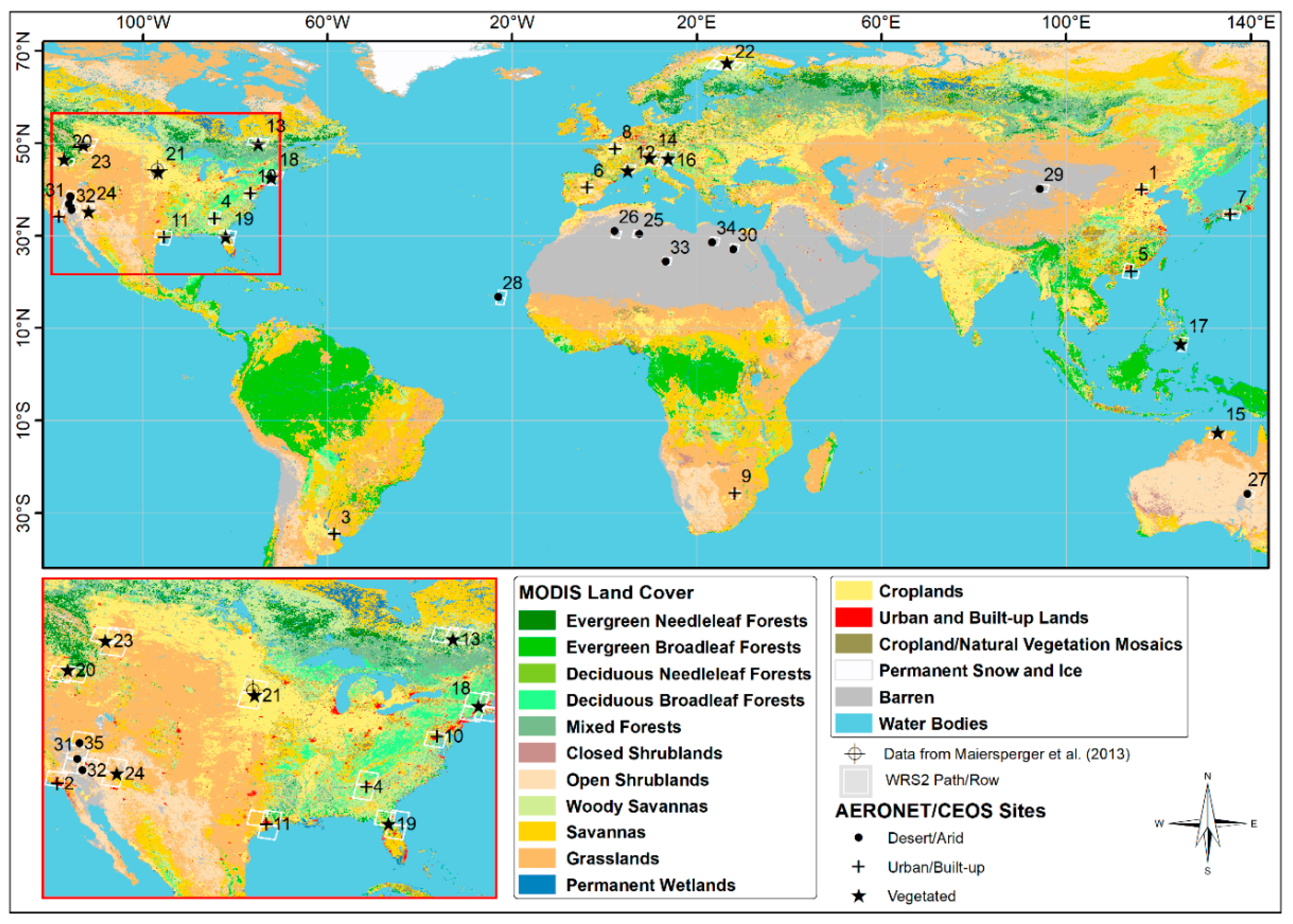
2.3. Site Selection for Comparison Purpose

In order to compare the SREM with the standard algorithms, e.g. LEDAPS and LaSRC, three broad land cover types (urban, vegetation, and arid) are selected based on the global mosaics of the standard MODIS land cover type data product (MCD12Q1). This product describes land cover properties derived from yearly MODIS observations. The primary land cover scheme identifies 17 land cover classes defined by the International Geosphere Biosphere Programme (IGBP), which includes 11 natural vegetation classes, 3 developed and mosaicked land classes, and 3 nonvegetated land classes [4]. The spatially aggregated MODIS Collection 6 land cover product at a spatial resolution of 500 m [41] is obtained from the NASA Earthdata Search (https://search.earthdata.nasa.gov/) for the year 2017. A total of 35 AERONET (Aerosol Robotic Network) and CEOS pseudo-invariant and instrumented sites located in urban/built-up (11), vegetated (13) and arid/desert (11) regions are selected based on the MODIS land cover classification (Table 2). For the AERONET sites, only the L8 OLI sensor data were used (from 1 April, 2013 to 15 October, 2018), while for the CEOS sites, the L5 TM, L7 ETM+, and L8 OLI sensors data are used from January 2000 to May 2012, July 1999 to May 2003 (non-SLC affected data), and April 2013 to 15 October, 2018, respectively. For each selected site, the Landsat scenes are ordered through the ESPA on-demand interface (https://espa.cr.usgs.gov).

Table 2. Aerosol Robotic Network (AERONET) and Committee on Earth Observation Satellites (CEOS) sites involved in a comparison between the Landsat surface reflectance (Landsat Ecosystem Disturbance Adaptive Processing System (LEDAPS) and Landsat 8 Surface Reflectance Code (LaSRC)) and SREM.

S/N	Site Name	Longitude (dd)	Latitude (dd)	Land Cover	Subtype	Path/Row
1	Beijing a	116.38	39.98	Urban	Urban	123/32
2	CalTech a	−118.13	34.14	Urban	Near Coast	41/36
3	CEILAP-BA a	−58.51	−34.56	Urban	Urban	225/84
4	Georgia_Tech a	−84.40	33.78	Urban	Near Vegetation	19/36, 19/37
5	Hong_Kong_PolyU a	114.18	22.30	Urban	Urban	121/45, 122/44, 122/45
6	Madrid a	−3.72	40.45	Urban	Urban	201/32
7	Osaka a	135.59	34.65	Urban	Urban	109/36, 110/36
8	Paris a	2.36	48.85	Urban	Urban	199/26
9	Pretoria_CSIR-DPSS a	28.28	−25.76	Urban	Urban	170/78
10	UMBC a	−76.71	39.25	Urban	Urban	15/33
11	Univ_of_Houston a	−95.34	29.72	Urban	Urban	25/39, 25/40, 26/39
12	Carpentras a	5.06	44.08	Vegetation	Cropland	196/29
13	Chapais a	−74.98	49.82	Vegetation	Forest	16/25, 17/25
14	Davos a	9.84	46.81	Vegetation	Grassland	193/27, 193/28, 194/27
15	Jabiru a	132.89	−12.66	Vegetation	Savanna	104/69, 105/69
16	Kanzelhohe_Obs a	13.90	46.68	Vegetation	Forest	191/27, 191/28
17	ND_Marbel_Univ a	124.84	6.50	Vegetation	Cropland	112/55, 112/56
18	NEON_Harvard a	−72.17	42.54	Vegetation	Forest	13/30, 13/31, 12/30, 12/31
19	NEON_OSBS a	−81.99	29.69	Vegetation	Savanna	16/39, 16/40, 17/39
20	Rimrock a	−116.99	46.49	Vegetation	Savanna	42/28, 43/28
21	Sioux_Falls a	−96.63	43.74	Vegetation	Cropland	29/29, 29/30
22	Sodankyla a	26.63	67.37	Vegetation	Savanna	191/13, 190/13, 192/12, 192/13
23	Univ_of_Lethbridge a	−112.87	49.68	Vegetation	Grassland	40/25, 40/26, 41/25
24	USGS_Flagstaff_ROLO a	−111.63	35.21	Vegetation	Savanna	37/35, 37/36
25	Algeria 3 b	7.66	30.32	Desert	Arid	192/39
26	Algeria 5 b	2.23	31.02	Desert	Arid	195/39
27	Birdsville a	139.35	−25.90	Desert	Arid	98/78
28	Capo_Verde a	−22.94	16.73	Desert	Shrubland	209/48, 209/49
29	Dunhuang b	94.34	40.13	Desert	Arid	137/32
30	El_Farafra a	27.99	27.06	Desert	Barren	178/41
31	Frenchman_Flat a	−115.93	36.81	Desert	Barren	40/34, 40/35
32	Ivanpah Playa b	−115.40	35.57	Desert	Arid	39/35
33	Libya 1 b	13.35	24.42	Desert	Arid	187/43
34	Libya 4 b	23.39	28.55	Desert	Arid	181/40
35	Railroad Valley Playa b	−115.69	38.50	Desert	Arid	40/33

^a AERONET sites (L8 OLI sensor’s data was used from 1 April, 2013 to 15 October, 2018). ^b CEOS sites (L5 TM, L7ETM+ and L8 OLI sensors data were used from 1 January, 2000 to 15, October 2018).

Table 2. Aerosol Robotic Network (AERONET) and Committee on Earth Observation Satellites (CEOS) sites involved in a comparison between the Landsat surface reflectance (Landsat Ecosystem Disturbance Adaptive Processing System (LEDAPS) and Landsat 8 Surface Reflectance Code (LaSRC)) and SREM.

S/N	Site Name	Longitude (dd)	Latitude (dd)	Land Cover	Subtype	Path/Row
1	Beijing a	116.38	39.98	Urban	Urban	123/32
2	CalTech a	−118.13	34.14	Urban	Near Coast	41/36
3	CEILAP-BA a	−58.51	−34.56	Urban	Urban	225/84
4	Georgia_Tech a	−84.40	33.78	Urban	Near Vegetation	19/36, 19/37
5	Hong_Kong_PolyU a	114.18	22.30	Urban	Urban	121/45, 122/44, 122/45
6	Madrid a	−3.72	40.45	Urban	Urban	201/32
7	Osaka a	135.59	34.65	Urban	Urban	109/36, 110/36
8	Paris a	2.36	48.85	Urban	Urban	199/26
9	Pretoria_CSIR-DPSS a	28.28	−25.76	Urban	Urban	170/78
10	UMBC a	−76.71	39.25	Urban	Urban	15/33
11	Univ_of_Houston a	−95.34	29.72	Urban	Urban	25/39, 25/40, 26/39
12	Carpentras a	5.06	44.08	Vegetation	Cropland	196/29
13	Chapais a	−74.98	49.82	Vegetation	Forest	16/25, 17/25
14	Davos a	9.84	46.81	Vegetation	Grassland	193/27, 193/28, 194/27
15	Jabiru a	132.89	−12.66	Vegetation	Savanna	104/69, 105/69
16	Kanzelhohe_Obs a	13.90	46.68	Vegetation	Forest	191/27, 191/28
17	ND_Marbel_Univ a	124.84	6.50	Vegetation	Cropland	112/55, 112/56
18	NEON_Harvard a	−72.17	42.54	Vegetation	Forest	13/30, 13/31, 12/30, 12/31
19	NEON_OSBS a	−81.99	29.69	Vegetation	Savanna	16/39, 16/40, 17/39
20	Rimrock a	−116.99	46.49	Vegetation	Savanna	42/28, 43/28
21	Sioux_Falls a	−96.63	43.74	Vegetation	Cropland	29/29, 29/30
22	Sodankyla a	26.63	67.37	Vegetation	Savanna	191/13, 190/13, 192/12, 192/13
23	Univ_of_Lethbridge a	−112.87	49.68	Vegetation	Grassland	40/25, 40/26, 41/25
24	USGS_Flagstaff_ROLO a	−111.63	35.21	Vegetation	Savanna	37/35, 37/36
25	Algeria 3 b	7.66	30.32	Desert	Arid	192/39
26	Algeria 5 b	2.23	31.02	Desert	Arid	195/39
27	Birdsville a	139.35	−25.90	Desert	Arid	98/78
28	Capo_Verde a	−22.94	16.73	Desert	Shrubland	209/48, 209/49
29	Dunhuang b	94.34	40.13	Desert	Arid	137/32
30	El_Farafra a	27.99	27.06	Desert	Barren	178/41
31	Frenchman_Flat a	−115.93	36.81	Desert	Barren	40/34, 40/35
32	Ivanpah Playa b	−115.40	35.57	Desert	Arid	39/35
33	Libya 1 b	13.35	24.42	Desert	Arid	187/43
34	Libya 4 b	23.39	28.55	Desert	Arid	181/40
35	Railroad Valley Playa b	−115.69	38.50	Desert	Arid	40/33

^a AERONET sites (L8 OLI sensor’s data was used from 1 April, 2013 to 15 October, 2018). ^b CEOS sites (L5 TM, L7ETM+ and L8 OLI sensors data were used from 1 January, 2000 to 15, October 2018).

3. Methodology

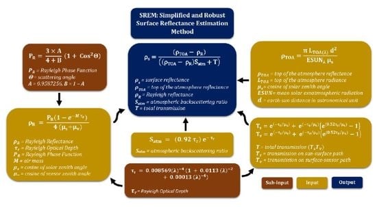
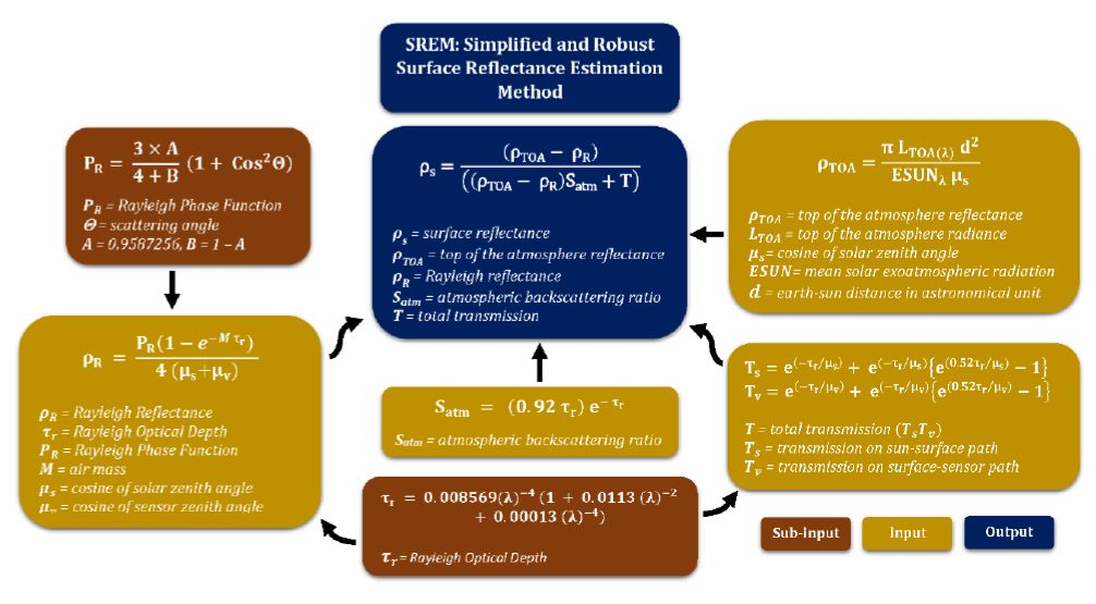
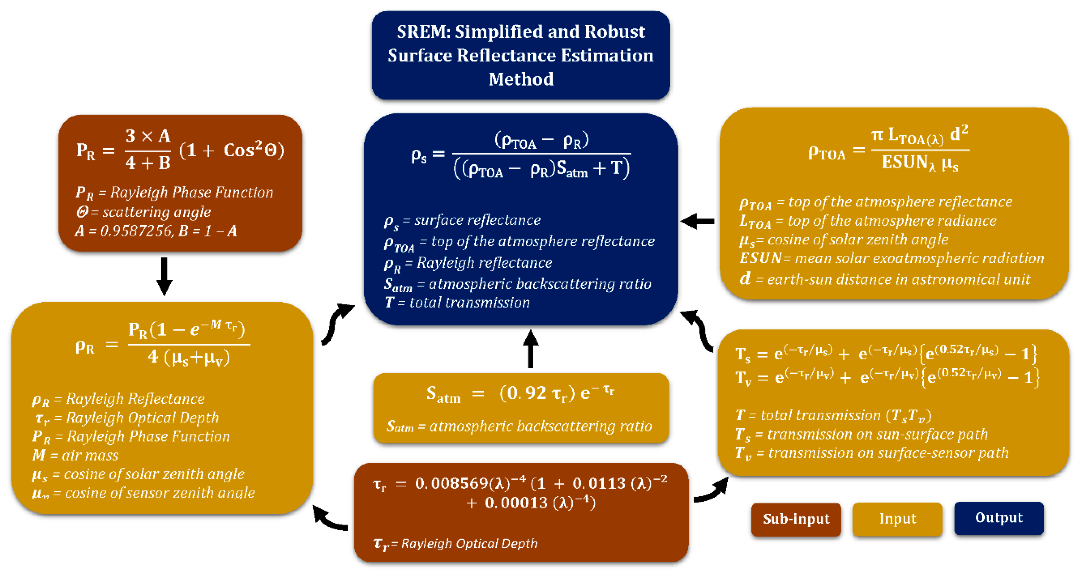
3.1. Surface Reflectance Inversion

In general, SR retrievals are derived from the TOA reflectance that can be simulated based on the following 6SV RT model equation (Equation (1)) for the Lambertian uniform target [17,20,42]:

$$\begin{array}{l}{\rho }_{TOA}\left(\lambda ,{\theta }_s,{\theta }_v,\phi ,{\tau }_a,{\omega }_a,P_A,U_{H_{2}O,}{U}_{O_3}\right)\\ =T{g}_{OG}T{g}_{O_3}[{\rho }_{atm}(\lambda ,{\theta }_s,{\theta }_v,\phi ,{\tau }_a,{\omega }_a,P_A,U_{H_{2}O})\\ +T_s\left(\lambda ,{\theta }_s,{\tau }_a,{\omega }_a,P_A\right)T_v\left(\lambda ,{\theta }_v,{\tau }_a,{\omega }_a,P_A\right)\frac{{\rho }_s\left(\lambda \right)}{1-S_{atm}\left(\lambda ,{\tau }_a,{\omega }_a,P_A\right){\rho }_s\left(\lambda \right)}T{g}_{H_{2}O}]\end{array}$$

(1)

where

• ${\rho }_{TOA}$ = reflectance received by satellite at the top of the atmosphere,
• ${\rho }_{atm}$ = atmospheric intrinsic path reflectance,
• $\lambda$ = wavelength
• $T_s$ = atmospheric transmittance of sun-surface path (downward),
• $T_v$ = atmospheric transmittance of surface-sensor path (upward),
• ${\rho }_s$ = surface reflectance to be estimated,
• $S_{atm}$ = atmospheric backscattering ratio to count multiple reflections between the surface and atmosphere,
• ${\theta }_s$ = solar zenith angle,
• ${\theta }_v$ = sensor zenith angle,
• $\phi$ = relative azimuth angle,
• $U_{H_{2}O,}$ = the integrated water vapor content,
• $U_{O_3,}$ = the integrated ozone content,
• ${\tau }_a,{\omega }_a,P_A$ = aerosol optical depth, aerosol single scatter albedo, and aerosol phase function, respectively, and
• $T{g}_{H_{2}O},T{g}_{O_3},T{g}_{OG}$ = gaseous transmission by water vapor, ozone, and other gases, respectively.

The atmospheric intrinsic reflectance can be approximated using Equation (2) [17]:

$${\rho }_{atm}\left(\lambda ,{\theta }_s,{\theta }_v,\phi ,{\tau }_a,{\omega }_a,P_A,U_{H_{2}O}\right)={\rho }_R\left(\lambda ,{\theta }_s,{\theta }_v,\phi \right)+\left({\rho }_{A+R}\left(\lambda ,{\theta }_s,{\theta }_v,\phi \right)-{\rho }_R\left(\lambda ,{\theta }_s,{\theta }_v,\phi \right)\right)T{g}_{H_{2}O}$$

(2)

where

• ${\rho }_R$ = atmospheric reflectance due to Rayleigh scattering and
• ${\rho }_{A+R}$ = combined atmospheric reflectance due to Rayleigh and aerosols.

The objective of this study is to perform an SR inversion using an equation based on the 6SV RT model without using aerosol information such as ${\tau }_a,{\omega }_a,\mathrm{and}{P}_A$ (i.e., ${\rho }_A=0$) and other atmospheric parameters such as, $U_{H_{2}O,}$ $U_{O_3,}$ and OG (i.e., $T{g}_{OG},T{g}_{O_3},\mathrm{and}T{g}_{H_{2}O}=1)$. Therefore, these parameters are neglected on the right-hand sides of Equations (1) and (2), such that the TOA reflectance can be approximated as Equation (3):

$${\rho }_{TOA}\left(\lambda ,{\theta }_s,{\theta }_v,\phi ,{\tau }_a,{\omega }_a,P_A\right)={\rho }_R\left(\lambda ,{\theta }_s,{\theta }_v,\phi \right)+T_s\left(\lambda \right)T_v\left(\lambda \right)\frac{{\rho }_s\left(\lambda \right)}{1-S_{atm}\left(\lambda \right){\rho }_s\left(\lambda \right)}$$

(3)

From Equation (3), ${\rho }_s$ for the SREM method is approximated as Equation (4), and for simplicity, Equation (4) is expressed as Equation (5):

$${\rho }_s\left(\lambda \right)=\frac{{\rho }_{TOA}\left(\lambda ,{\theta }_s,{\theta }_v,\phi ,{\tau }_a,{\omega }_a,P_A\right)-{\rho }_R\left(\lambda ,{\theta }_s,{\theta }_v,\phi \right)}{\left({\rho }_{TOA}\left(\lambda ,{\theta }_s,{\theta }_v,\phi ,{\tau }_a,{\omega }_a,P_A\right)-{\rho }_R\left(\lambda ,{\theta }_s,{\theta }_v,\phi \right)\right)S_{atm}\left(\lambda \right)+T_s\left(\lambda \right)T_v\left(\lambda \right)}$$

(4)

$${\rho }_s=\frac{{\rho }_{TOA}-{\rho }_R}{\left({\rho }_{TOA}-{\rho }_R\right)S_{atm}+T_s{T}_v}$$

(5)

where ${\rho }_s$ = SREM estimated surface reflectance.

It should be noted that SREM SR is different than the Rayleigh corrected TOA reflectance, which can be obtained by simple subtraction of Rayleigh reflectance from the TOA reflectance.

In Equation (4), the TOA reflectance and Rayleigh reflectance is computed using Equations (6) and (7) [43], respectively:

$${\rho }_{TOA}\left(\lambda ,{\theta }_s,{\theta }_v,\phi ,{\tau }_a,{\omega }_a,P_A\right)=\frac{\pi L_{TOA}\left(\lambda ,{\theta }_s,{\theta }_v,\phi \right)d^2}{ESU{N}_{\lambda }{\mu }_s}$$

(6)

where

• $L_{TOA}$ = radiance received by satellite at the top of the atmosphere,
• $d$ = distance between the Earth and Sun in the astronomical unit,
• $ESUN$ = mean solar exoatmospheric radiation,
• ${\mu }_s$ = cosine of solar zenith angle, and
• $\lambda$ = wavelength.

$${\rho }_R\left(\lambda ,{\theta }_s,{\theta }_v,\phi \right)=P_R\left({\theta }_s,{\theta }_v,\phi \right)\frac{\left(1-e^{-M{\tau }_r}\right)}{4({\mu }_s+{\mu }_v)}$$

(7)

where

• $M$ = air mass calculated using Equation (8) [43],
• ${\tau }_r$ = Rayleigh optical depth calculated using Equation (9) [44],
• $P_R$ = Rayleigh phase function calculated using Equation (10) [43], and
• ${\mu }_v$ = cosine of sensor zenith angle.

$$M=\frac{1}{{\mu }_s}+\frac{1}{{\mu }_v}$$

(8)

$${\tau }_r=0.008569{\left(\lambda \right)}^{-4}\left(1+0.0113{\left(\lambda \right)}^{-2}+0.0013{\left(\lambda \right)}^{-4}\right)$$

(9)

$$P_R=\frac{3A}{4+B}\left(1+co{s}^2\Theta \right);A=0.9587256,B=1-A$$

(10)

where

• $\Theta$ = scattering angle, and
• A and B are coefficients that account for the molecular asymmetry.

In Equation (4), the atmospheric backscattering ratio and total atmospheric transmission, without integrating aerosol information, is expressed as Equations (11)–(13) [7,45,46], respectively:

$$S_{atm}\left(\lambda \right)=\left(0.92{\tau }_r\right)e^{-{\tau }_r}$$

(11)

$$T_s\left(\lambda \right)=e^{\left(-{\tau }_r/{\mu }_s\right)}+e^{(-{\tau }_r/{\mu }_s)}\left\{e^{(0.52{\tau }_r/{\mu }_s)}-1\right\}$$

(12)

$$T_v\left(\lambda \right)=e^{\left(-{\tau }_r/{\mu }_v\right)}+e^{(-{\tau }_r/{\mu }_v)}\left\{e^{(0.52{\tau }_r/{\mu }_v)}-1\right\}$$

(13)

The SREM SR retrievals were estimated for each Landsat band (TM and ETM+: B1-B5 and B7, and OLI: B1-B7) using Equation (4), and for a clear understanding of the SREM, the step-by-step methodology is described in Figure 2.

3.2. Evaluation Process

The SREM is validated against a range of criteria and features, extensive in itself, in order to test its robustness and explore its potential application. The evaluation process comprises eight steps: (1) The SREM estimated SR and LEDAPS (TM5 and ETM+) SR observations are compared with in situ SR measurements collected by Maiersperger, Scaramuzza, Leigh, Shrestha, Gallo, Jenkerson, and Dwyer [35]. The SREM and LEDAPS SR retrievals are averaged from the spatial window of 3 × 3 pixels if at least 2 out of 9 pixels are available centered on the measurement site. (2) The SREM and Landsat (LEDAPS and LaSRC) SR retrievals are compared for 35 sites located over urban (2013–2018), vegetated (2013–2018), and desert surfaces (2000 to 2018) (Figure 1 and Table 2). To obtain the collocated SREM and Landsat data, (i) retrievals are filtered for the quality flag “66” (clear and low-confidence cloud) for LEDAPS and “322” (clear and low-confidence cloud) for LaSRC, and (ii) matched for the same time and location. (3) In order to evaluate the performance of the SR inversion methods during different aerosol loadings, SR retrievals for each channel were filtered based on the AOD at 550 nm obtained from AERONET sites. (4) A spatio-temporal cross-comparison is conducted for six Landsat paths/rows (122/44, 199/26, 201/32, 170/78, 15/33, and 25/39) located over different regions and climatic zones. For a comprehensive comparison for diverse land surfaces and varying atmospheric conditions, 3000 data points are randomly selected from each image-pair of SREM and LaSRC for each path/row. For this comparison, those Landsat retrievals, that may have values outside the theoretical limits, i.e., 0 < SR < 1, are removed. These unusual retrievals are available due to over-correction for atmosphere and Landsat calibration errors [47,48,49,50] or retrievals with SR > 1 might be available for those surfaces that reflect more strongly than Lambertian surfaces [51]. (5) The Normalized Difference Vegetation Index (NDVI, Equation (14)) [1,52], Enhanced Vegetation Index (EVI, Equation (15)) [1], and Soil Adjusted Vegetation Index (SAVI, Equation (16)) [1] are calculated using SREM and Landsat SR data and compared with each other to demonstrate the ability of the SREM to monitor vegetation and crops.

$$NDVI=\frac{\left(NIR-Red\right)}{\left(NIR+Red\right)}$$

(14)

$$EVI=2.5\times \left\{\frac{\left(NIR-Red\right)}{\left(NIR+6\times Red-7.5\times Blue+1\right)}\right\}$$

(15)

$$SAVI=1.5\times \left\{\frac{\left(NIR-Red\right)}{\left(NIR+Red+0.5\right)}\right\}$$

(16)

(6) To further explore its applicability, the SREM is applied to the Sentinel-2A and MODIS datasets and compared with the Sentinel-2A SR observations estimated by the latest version (2.5.5) of the Sen2Cor and MOD09 level 2 surface reflectance products, respectively. For this purpose, Beijing, a city with mixed bright urban surfaces that mostly remains under frequent haze and dust pollution effects, is selected as a test site. (7) In order to calculate the slope and intercept between the SREM and Landsat retrievals, the reduced major axis (RMA) is used, which can simultaneously account for errors in both dependent and independent variables [53,54]. In RMA, slope (β) and intercept (α) are determined using Equations (17) and (18):

$$\beta =\frac{{\sigma }_y}{{\sigma }_x}$$

(17)

$$\alpha =\overline{Y}-\left(\frac{{\sigma }_y}{{\sigma }_x}\right)\overline{X}$$

(18)

where

• $\overline{X}$ and $\overline{Y}$ = means of X and Y, respectively, and
• ${\sigma }_x$ and ${\sigma }_y$ = standard deviations of X and Y, respectively.

(8) To report the consistency and errors in the SREM SR product, the Pearson’s correlation coefficient (r), mean bias error (MBE, Equation (19)), root-mean-squared difference (RMSD, Equation (20)), and mean systematic error (MSE, Equation (21)) are computed. The MSE is useful to report the difference between the trend of X and Y data; small MSE indicates a good trend.

$$MBE=\frac{1}{n}{\displaystyle \sum }_{i=1}^n\left(Y_i-X_i\right)$$

(19)

$$RMSD=\sqrt{\frac{1}{n}{\displaystyle \sum }_{i=1}^n{\left(Y_i-X_i\right)}^2}$$

(20)

$$MSE=\frac{1}{n}{\displaystyle \sum }_{i=1}^n{\left({\widehat{Y}}_i-X_i\right)}^2$$

(21)

where $\widehat{Y}$ = predicted value based on RMA relationship (Y = βX + α) between X and Y.

4. Results and Discussion

4.1. Cross-Comparison of ASD, LEDAPS, and SREM SR Data

The SR data collected by ASD for the SDSU site are available for only 10 days [35] (Appendix A) and are compared with the LEDAPS and SREM SR retrievals (

Table 3. Validation summary of LEDAPS and SREM SR retrievals against Analytical Spectral Devices (ASD) FieldSpec spectrometer data.

Date	Sensor	Band 1			Band 2			Band 3
		ASD	LEDAPS	SREM	ASD	LEDAPS	SREM	ASD	LEDAPS	SREM
20030826	ETM+	0.045	0.053	0.067	0.075	0.080	0.076	0.086	0.090	0.085
20060615	ETM+	0.054	0.063	0.078	0.092	0.099	0.094	0.106	0.108	0.102
20070720	ETM+	0.051	0.057	0.070	0.085	0.091	0.087	0.110	0.116	0.110
20080612	TM5	0.072	0.063	0.073	0.114	0.105	0.096	0.123	0.108	0.087
20080714	TM5	0.056	0.058	0.068	0.086	0.095	0.088	0.108	0.111	0.101
20080823	ETM+	0.051	0.052	0.064	0.080	0.080	0.076	0.093	0.092	0.104
20080916	TM5	0.037	0.054	0.063	0.059	0.083	0.076	0.068	0.100	0.093
20090530	TM5	0.052	0.055	0.065	0.087	0.090	0.084	0.084	0.087	0.057
20100805	TM5	0.030	0.040	0.056	0.057	0.067	0.066	0.052	0.057	0.418
20100821	TM5	0.030	0.037	0.052	0.059	0.068	0.066	0.054	0.058	0.359
Average		0.048	0.053	0.066	0.079	0.086	0.081	0.088	0.093	0.088
1 StDev		0.012	0.008	0.007	0.017	0.012	0.010	0.023	0.020	0.018
2 CV		0.255	0.154	0.108	0.212	0.138	0.126	0.261	0.214	0.201
MBE			0.005	0.018		0.006	0.002		0.004	0.000
r			0.869	0.809		0.905	0.914		0.883	0.888
Date	Sensor	Band 4			Band 5			Band 7
		ASD	LEDAPS	SREM	ASD	LEDAPS	SREM	ASD	LEDAPS	SREM
20030826	ETM+	0.277	0.276	0.253	0.319	0.310	0.289	0.172	0.174	0.148
20060615	ETM+	0.312	0.299	0.268	0.317	0.296	0.271	0.170	0.163	0.135
20070720	ETM+	0.259	0.256	0.239	0.344	0.338	0.318	0.197	0.206	0.179
20080612	TM5	0.328	0.301	0.281	0.317	0.289	0.262	0.174	0.153	0.136
20080714	TM5	0.246	0.277	0.254	0.335	0.323	0.289	0.203	0.186	0.163
20080823	ETM+	0.280	0.264	0.248	0.335	0.324	0.305	0.183	0.183	0.159
20080916	TM5	0.236	0.244	0.225	0.277	0.300	0.269	0.148	0.175	0.153
20090530	TM5	0.307	0.280	0.263	0.295	0.282	0.258	0.159	0.156	0.140
20100805	TM5	0.315	0.317	0.284	0.233	0.226	0.199	0.109	0.105	0.090
20100821	TM5	0.339	0.334	0.299	0.236	0.227	0.200	0.106	0.095	0.082
Average		0.290	0.285	0.261	0.301	0.292	0.266	0.162	0.160	0.138
StDev		0.034	0.026	0.021	0.038	0.036	0.038	0.031	0.033	0.029
CV		0.116	0.930	0.815	0.125	0.125	0.142	0.193	0.208	0.210
MBE			−0.005	−0.028		−0.009	−0.035		−0.002	−0.024
r			0.878	0.919		0.944	0.949		0.921	0.922

¹ StDev = Standard deviation. ² CV = Coefficient of variations (StDev/average).

). Table 3 shows comparable values of Pearson’s correlation coefficient (r) for LEDAPS and SREM with ASD data. Overestimation is observed in LEDAPS from B1 to B3, and underestimation in SREM is from B4 to B7. The maximum positive MBE for LEDAPS is 0.006 for B2 and for SREM it is 0.018 for B1. Similarly, the maximum negative MBE is for B5, with −0.009 and −0.035 for LEDAPS and SREM, respectively. The results for SREM are satisfactory with a high value of r and the reason for large negative values of MBE are investigated in the following analysis.

For this purpose, LEDAPS and SREM SR retrievals are compared with the TOA reflectance observations obtained for the same dates (

Table 4. Summary of cross-comparison between LEDAPS and SREM SR retrievals and top of atmosphere (TOA) reflectance observations.

Bands	Average			MBE		R
	TOA	LEDAPS	SREM	LEDAPS	SREM	LEDAPS	SREM
B1	0.107	0.053	0.066	−0.054	−0.041	0.963	0.997
B2	0.104	0.086	0.081	−0.018	−0.023	0.994	0.999
B3	0.100	0.093	0.088	−0.008	−0.013	1.000	1.000
B4	0.265	0.285	0.261	0.020	−0.003	0.984	1.000
B5	0.266	0.292	0.266	0.025	0.000	0.993	1.000
B7	0.139	0.160	0.138	0.021	−0.001	0.995	1.000

). The hypothesis of this analysis is that the method, LEDAPS or SREM, with the larger negative value of MBE would be considered as superior, as it represents the greater removal of atmospheric effects. On the other hand, a large positive value represents “under-correction”; hence, the respective method is unable to remove atmospheric effects significantly. The results (Table 4) show that LEDAPS has a larger negative MBE for B1 compared to SREM, whereas, SREM has a larger negative MBE for B2 and B3 than LEDAPS, which indicate the better performances of LEDAPS for B1 and SREM for B2 and B3. For B4 to B7, LEDAPS has larger positive values of MBE than SREM, which might be due to its sensitivity to the absorption by atmospheric gases in the infrared spectral region and shows “under correction (lack of atmospheric correction)” of LEDAPS. These results (Table 3 and Table 4) suggest that SREM is less sensitive to the absorption by atmospheric gases and performs within the expected range, as the average values of SR retrievals are less than the TOA reflectance, whereas LEDAPS values are even greater than the TOA reflectance; especially, for B4 to B7. Therefore, it can be concluded that SREM, without integrating aerosol information and a comprehensive precalculated LUT in the inversion, can provide SR retrievals that are comparable with both the ASD and LEDAPS observations.

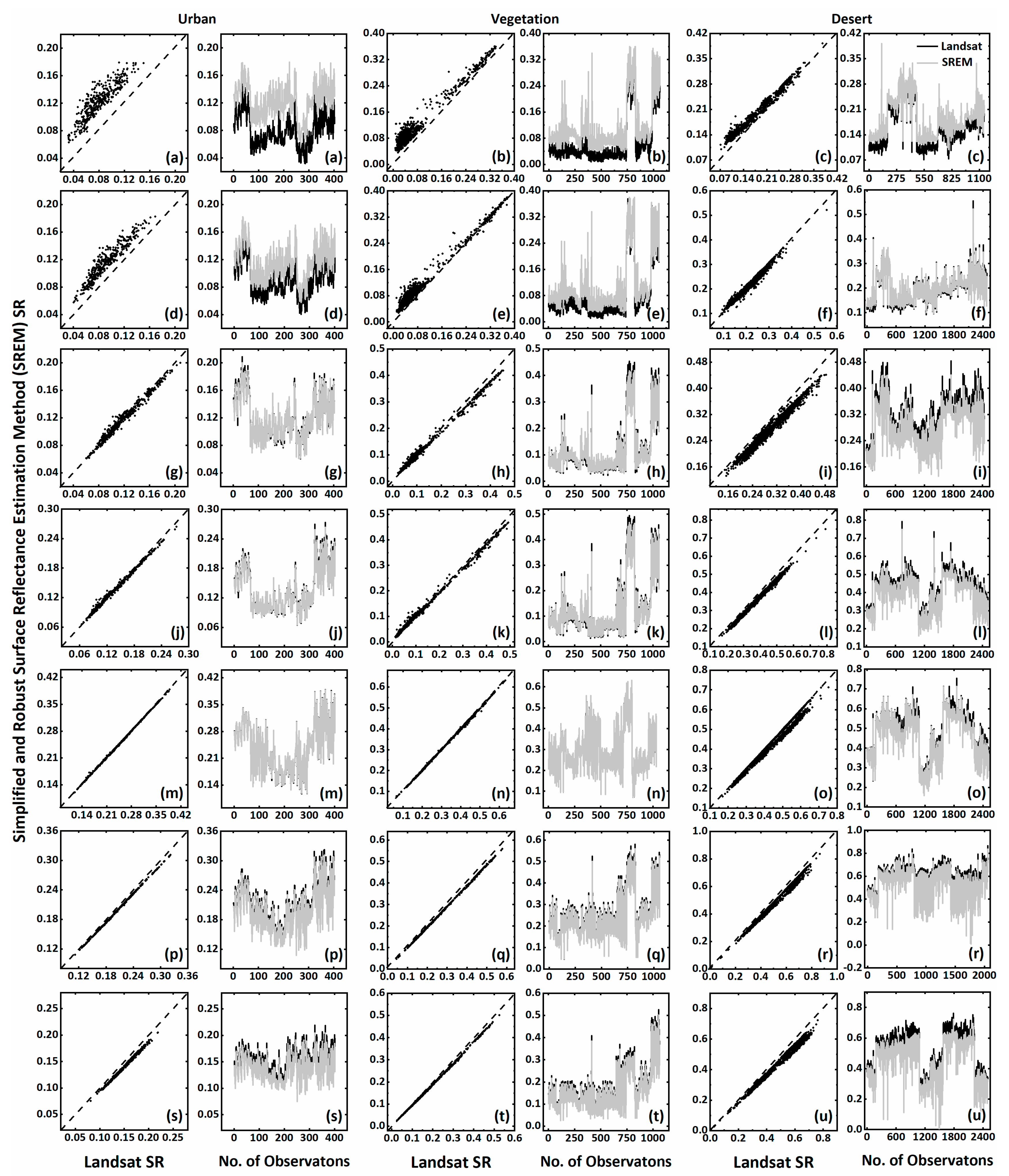
4.2. Cross-Comparison between SREM and Landsat SR Retrievals

A cross-comparison between SREM and Landsat (LEDAPS and LaSRC) SR retrievals is conducted over urban as well as vegetated surfaces from 2013 to 2018, and desert (arid) surfaces from 2000 to 2018. Figure 3 shows the scatter (dashed line = 1:1 line) and line plots (black line = Landsat, gray line = SREM) between SREM and Landsat retrievals. The results are summarized in

Table 5. Summary of cross-comparison between coincident SREM and Landsat (LEDAPS and LaSRC) SR retrievals over urban and vegetated sites from 2013–2018, and desert (arid) sites from 2000–2018.

1 LC	2 TP	Sensor	Band	3 n	4 β	5 α	6 r	MBE	RMSD	MSE
Urban	2013–2018	OLI	Coastal Aerosol	402	1.057	0.037	0.891	0.042	0.044	0.002
			Blue	402	1.018	0.022	0.951	0.024	0.025	0.001
			Green	402	0.943	0.006	0.990	−0.001	0.005	0.000
			Red	402	0.939	0.007	0.997	−0.002	0.005	0.000
			NIR	402	0.989	0.003	1.000	0.000	0.001	0.000
			SWIR1	402	0.972	−0.002	1.000	−0.007	0.008	0.000
			SWIR2	402	0.949	−0.003	0.997	−0.01	0.011	0.000
			All	2814	0.874	0.025	0.963	0.006	0.020	0.000
Vegetation	2013–2018	OLI	CA	1062	0.928	0.043	0.983	0.038	0.041	0.001
			B	1056	0.931	0.027	0.991	0.021	0.025	0.000
			G	1056	0.904	0.008	0.997	−0.003	0.012	0.000
			R	1056	0.929	0.007	0.998	−0.002	0.010	0.000
			NIR	1032	0.989	0.002	1.000	−0.001	0.003	0.000
			SWIR1	1056	0.966	−0.001	1.000	−0.009	0.010	0.000
			SWIR2	1056	0.944	−0.002	1.000	−0.011	0.012	0.000
			All	7374	0.919	0.018	0.990	0.005	0.020	0.000
Desert	2013–2018	OLI	CA	1148	0.914	0.036	0.991	0.022	0.024	0.001
	2000–2018	TM ETM + OLI	B	2482	0.927	0.018	0.990	0.004	0.009	0.000
			G	2440	0.929	−0.002	0.991	−0.024	0.026	0.001
			R	2516	0.954	−0.007	0.997	−0.026	0.027	0.001
			NIR	2520	0.975	−0.006	0.990	−0.018	0.024	0.000
			SWIR1	2065	0.967	−0.011	0.995	−0.029	0.032	0.001
			SWIR2	2499	0.900	0.002	0.994	−0.048	0.052	0.003
			All	15789	0.907	0.016	0.994	−0.020	0.031	0.001

¹ LC = Land cover; ² TP = Time Period; ³ n = Total number of observations; ⁴ β = Slope; ⁵ α = Intercept; ⁶ r = Pearson’s correlation.

which shows that the SREM SR retrievals for coastal aerosol (Figure 3a–c) and blue (Figure 3d–f) spectral bands over desert (arid) sites (Figure 3d,f) are well correlated with the LaSRC and LEDAPS SR retrievals with r ~ 0.990–0.991 (Table 5), and small values of MBE ~ 0.004–0.022, and RMSD ~ 0.009–0.024, compared with urban (Figure 3a,d) and vegetated sites (Figure 3b,e). The values of MSE ~ 0.000–0.002 indicate only minor differences between the trend of SREM and Landsat (LaSRC and LEDAPS) retrievals independent from the surface type. The performance of the SREM for the blue band is better than for the coastal aerosol band with significant small values of MBE and RMSD. The SREM retrievals appear overestimated as indicated by the positive values of MBE, and these values over urban and vegetated sites are high compared to the results from desert sites and are acceptable according to previous studies [31,32,48]. Overestimation in coastal aerosol and blue bands may be due to the enhanced aerosol extinction and Rayleigh contribution in these wavelengths.

The performance of the SREM for green, red, NIR, SWIR1, and SWIR2 bands over the urban and vegetated sites is robust with r ~ 0.951–1.00, MBE ~ −0.01–0.011, RMSD ~ 0.001–0.012, and MSE ~ 0.00. The low values of MBE, RMSD, and MSE represent (i) very small differences between the SREM and Landsat retrievals, (ii) scatter points close to the 1:1 line, and (iii) minimal differences between the trend of SREM and Landsat SR retrievals. The comparison of all these bands over the desert sites was relatively less reliable with larger differences (MBE and RMSD) due to underestimation in the SREM retrievals, especially for SR > 0.50. The underestimation in the SREM retrievals in comparison with Landsat, especially for the desert surfaces, might be due to the “under-correction” of the Landsat atmospheric correction algorithm as observed in Section 4.1, which describes the cross-comparison between SR retrievals and TOA reflectance observations. Therefore, overall performance of the SREM appears robust, as results show a high consistency in the SREM with very high values of r, and small values of MBE and RMSD which suggest that the SREM renders consistent spatial (i.e., from site to site) and temporal (i.e., from 2000 to 2018) variations in SR as generated by LaSRC and LEDAPS products over heterogeneous surfaces.

To investigate the underestimation in the SREM retrievals over the desert sites for green to SWIR2 bands, cross-comparisons between the Landsat (LEDAPS and LaSRC) and SREM SR retrievals and TOA reflectance observations are conducted, similar to that in Section 4.1. The results (

Table 6. Summary of cross-comparison between Landsat (LEDAPS and LaSRC) and SREM SR retrievals and TOA reflectance observations over desert sites.

Bands	Average			MBE		r
	TOA	Landsat	SREM	Landsat	SREM	Landsat	SREM
Coastal Aerosol	0.268	0.217	0.238	−0.051	−0.030	0.997	0.998
Blue	0.284	0.256	0.261	−0.028	−0.023	0.998	0.998
Green	0.350	0.364	0.338	0.014	−0.012	0.997	0.998
Red	0.433	0.451	0.427	0.017	−0.006	0.997	0.998
NIR	0.517	0.520	0.517	0.003	0.000	0.994	0.995
SWIR1	0.582	0.607	0.585	0.025	0.003	0.977	0.982
SWIR2	0.499	0.525	0.498	0.036	−0.001	0.977	0.990

) show that the Landsat retrievals have positive MBE of 0.014 for green, 0.017 for red, 0.025 for SWIR1, and 0.036 for SWIR2 bands, compared with the SREM retrievals which are within the expected range of below or equal to TOA. These results represent “under-correction” of data by the Landsat atmospheric correction algorithms which might be due to their sensitivity to the atmospheric scattering and absorption in the visible and infrared spectral regions, respectively. Therefore, these results suggest that the apparent “underestimation” in the SREM retrievals over desert sites when compared to Landsat, is mainly due to the under-correction (positive bias) of the Landsat retrievals.

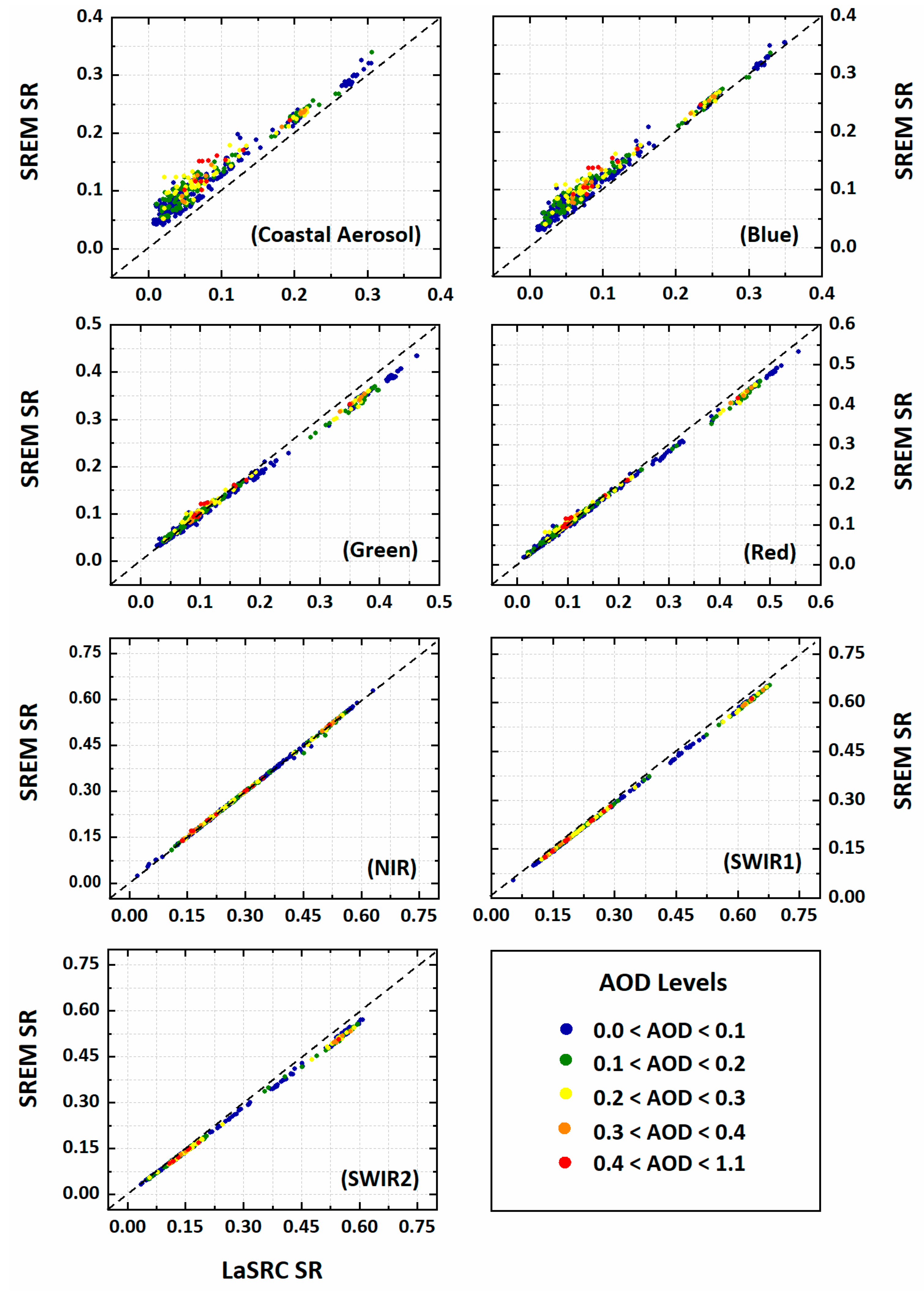
4.3. Impact of Aerosol Particles on SR Retrievals

In order to evaluate the performance of the SREM method during low to high aerosol loadings, the SR retrievals for each band are filtered based on five levels of AOD at 550 nm obtained from the AERONET sites, i.e., (i) 0.0 < AOD < 0.1, (ii) 0.1 < AOD < 0.2, (iii) 0.2 < AOD < 0.3, (iv) 0.3 < AOD < 0.4, and (v) 0.4 < AOD < 1.1. The results are presented in Figure 4, where different colors represent different levels of AOD. The cross-comparison is summarized in

Table 7. Statistical summary of cross-comparison between coincident Landsat and SREM SR retrievals for low to high AOD levels.

Band	1 AOD	2 n	3 β	4 α	5 r	MBE	RMSD
Coastal Aerosol	0.0 < AOD < 0.1	319	0.920	0.041	0.987	0.035	0.038
	0.1 < AOD < 0.2	125	0.893	0.049	0.985	0.039	0.042
	0.2 < AOD < 0.3	56	0.835	0.060	0.963	0.045	0.049
	0.3 < AOD < 0.4	13	0.864	0.055	0.988	0.039	0.042
	0.4 < AOD < 1.1	12	0.903	0.060	0.881	0.052	0.055
Blue	0.0 < AOD < 0.1	319	0.933	0.025	0.994	0.019	0.022
	0.1 < AOD < 0.2	125	0.906	0.032	0.995	0.021	0.025
	0.2 < AOD < 0.3	56	0.871	0.040	0.985	0.026	0.030
	0.3 < AOD < 0.4	13	0.894	0.036	0.997	0.021	0.024
	0.4 < AOD < 1.1	12	0.914	0.040	0.955	0.031	0.034
Green	0.0 < AOD < 0.1	319	0.913	0.007	0.999	−0.005	0.013
	0.1 < AOD < 0.2	125	0.899	0.011	0.999	−0.005	0.014
	0.2 < AOD < 0.3	56	0.890	0.015	0.998	−0.002	0.013
	0.3 < AOD < 0.4	13	0.905	0.013	1.000	−0.006	0.014
	0.4 < AOD < 1.1	12	0.906	0.016	0.995	0.003	0.010
Red	0.0 < AOD < 0.1	319	0.938	0.005	1.000	−0.005	0.011
	0.1 < AOD < 0.2	125	0.926	0.009	1.000	−0.005	0.013
	0.2 < AOD < 0.3	56	0.923	0.011	0.999	−0.003	0.012
	0.3 < AOD < 0.4	13	0.932	0.009	1.000	−0.007	0.013
	0.4 < AOD < 1.1	12	0.925	0.013	0.998	0.001	0.009
NIR	0.0 < AOD < 0.1	319	0.991	0.001	1.000	−0.002	0.002
	0.1 < AOD < 0.2	125	0.986	0.003	1.000	−0.002	0.003
	0.2 < AOD < 0.3	56	0.985	0.004	1.000	−0.001	0.003
	0.3 < AOD < 0.4	13	0.987	0.004	1.000	0.000	0.003
	0.4 < AOD < 1.1	12	0.981	0.006	1.000	0.001	0.004
SWIR1	0.0 < AOD < 0.1	319	0.964	−0.001	1.000	−0.011	0.012
	0.1 < AOD < 0.2	125	0.960	0.001	1.000	−0.012	0.014
	0.2 < AOD < 0.3	56	0.961	0.001	1.000	−0.011	0.013
	0.3 < AOD < 0.4	13	0.963	0.000	1.000	−0.013	0.015
	0.4 < AOD < 1.1	12	0.964	0.000	1.000	−0.008	0.009
SWIR2	0.0 < AOD < 0.1	319	0.935	−0.001	1.000	−0.014	0.018
	0.1 < AOD < 0.2	125	0.927	0.000	1.000	−0.017	0.022
	0.2 < AOD < 0.3	56	0.930	−0.001	1.000	−0.016	0.020
	0.3 < AOD < 0.4	13	0.925	0.000	1.000	−0.021	0.026
	0.4 < AOD < 1.1	12	0.925	0.000	1.000	−0.013	0.015

¹ AOD = AERONET AOD at 550 nm; ² n = Total number of observations; ³ β = Slope; ⁴ α = Intercept; ⁵ r = Pearson’s correlation.

, showing that the number of coincident retrievals decreases with the increase in AOD levels. Figure 4 shows that most of the scatter points for each band are close to the 1:1 line and hence well correlated with each other with a value of r from 0.881 to 1.00. According to the statistical summary (Table 7), the values of MBE increase with the increase in aerosol loadings for the coastal aerosol and blue bands, which suggests that the accuracy of SR retrievals for these bands are affected by the aerosol loadings. However, no direct or linear relationship between MBE and aerosol loadings was observed for the other bands (green to SWIR2). This suggests that the performance of the SREM improves for longer wavelength bands (green to SWIR), independent of the aerosol load. Interestingly, it is observed for these bands that the MBE and RMSD for high aerosol loading (0.4 < AOD < 1.1) is smaller than for low aerosol loadings (0.0 < AOD < 0.1), which suggests that SREM retrievals are less sensitive to the high aerosol load. Overall, results are significant and robust, showing consistency between the SREM and LaSRC retrievals during low to high aerosol loadings, and these justify the application of SREM, without integrating information of aerosol particles and atmospheric gases, to estimate SR similar to the LaSRC product.

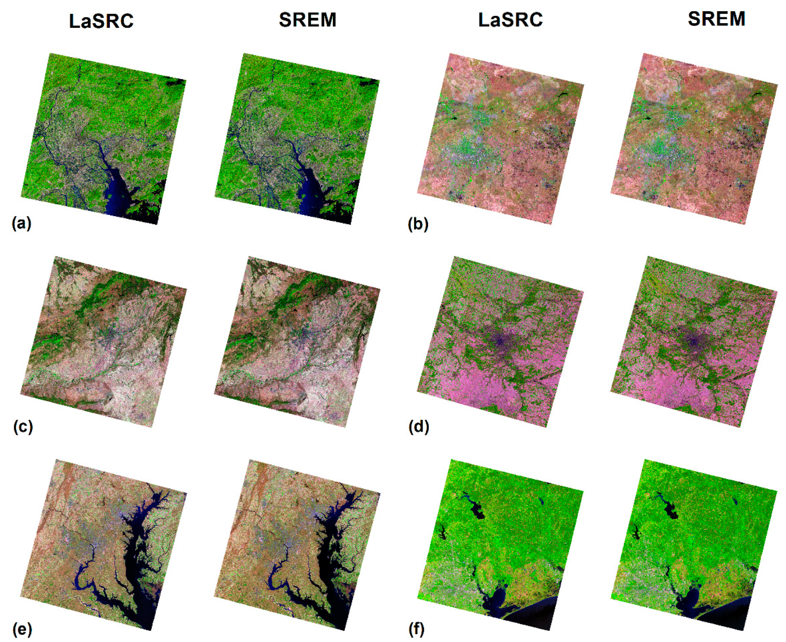
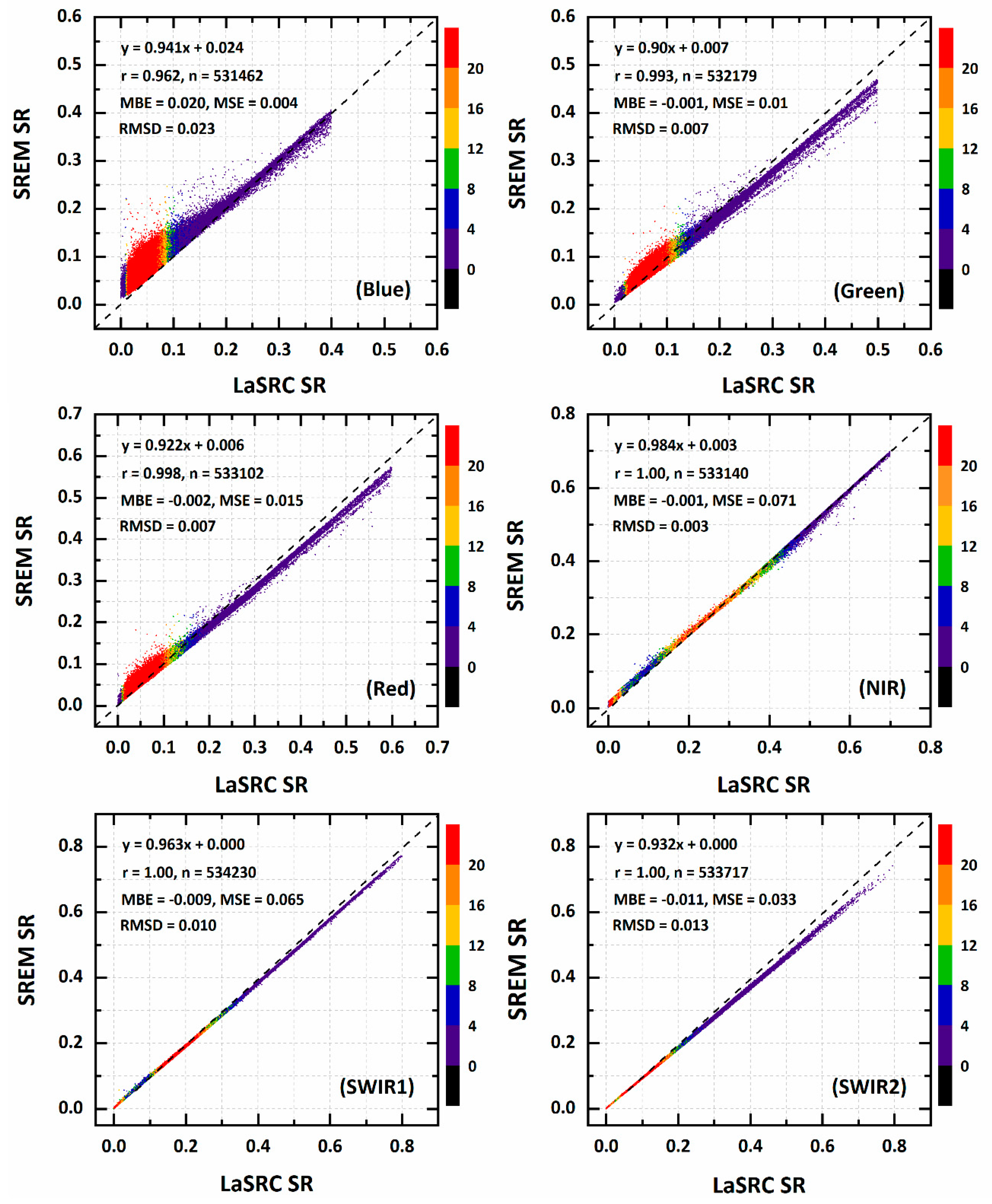
4.4. Spatio-Temporal Cross-Comparison between SREM and LaSRC Data

For performing spatial cross-comparison between SREM and Landsat SR products, six paths/rows located in Asia (122/44), Africa (170/78), Europe (119/26 and 201/32), and the United States of America (15/33 and 25/39) are selected to represent the diversity of land cover types, and climatic as well as air quality conditions. Figure 5 shows the LaSRC (Landsat 8) and SREM SR displayed as RGB false composites of bands 6, 5, 4, and the results indicate that the SREM yields SR images, which are spatially comparable with the LaSRC SR images. A spatial differences map between SREM and Sentinel-2A SR retrievals for the mentioned paths/rows is added as Figure S1 (supplementary data). A careful visual comparison of any land cover feature, from any panel in Figure 5, exhibits strong alikeness and agreement. These results show that the SREM has the ability to remove atmospheric effects without incorporating atmospheric parameters and a precalculated comprehensive LUT based on the RTM.

Temporal analysis is also conducted to consider diverse surface types and atmospheric conditions by selecting 3000 random points from each image of each path/row. This approach found 13 (122/44), 66 (170/78), 21 (199/26), 52 (201/32), 22 (15/33), and 26 (25/39) image-pairs, from 2013 to 2018. Total numbers of coincident points for analysis are 531,462 for blue, 532,179 for green, 533,102 for red, 533,140 for NIR, 534230 for SWIR1, and 533,717 for SWIR2 bands (Figure 6). Overall, results reveal a very good correlation between SREM and LaSRC SR products, with r close to unity (r = 0.993 to 1.00) and small values of MBE ≤ −0.002 for green, red, and NIR bands. A large value of MBE (0.020) is observed for the blue band, which may be due to the enhanced aerosol extinction and Rayleigh contribution. The SREM retrievals for the SWIR1 and SWIR2 are also correlated well with LaSRC retrievals but a slight underestimation is found as indicated by the negative value of MBE (−0.009 to −0.011). This underestimation may be due to under-correction by the Landsat atmospheric correction algorithm as discussed in the previous sections on cross-comparison with TOA reflectance. This investigation considers Landsat data as a “true and standard” data for cross-comparison which in fact has its own uncertainties due to aerosol retrieval algorithm, cloud contamination, and under or over atmospheric correction [47,48,49,55]. Overall, all these findings demonstrate the robust promise of SREM to retrieve SR for diverse surfaces and under varying atmospheric conditions, without incorporating aerosol and atmospheric parameters, in good agreement with the Landsat SR product.

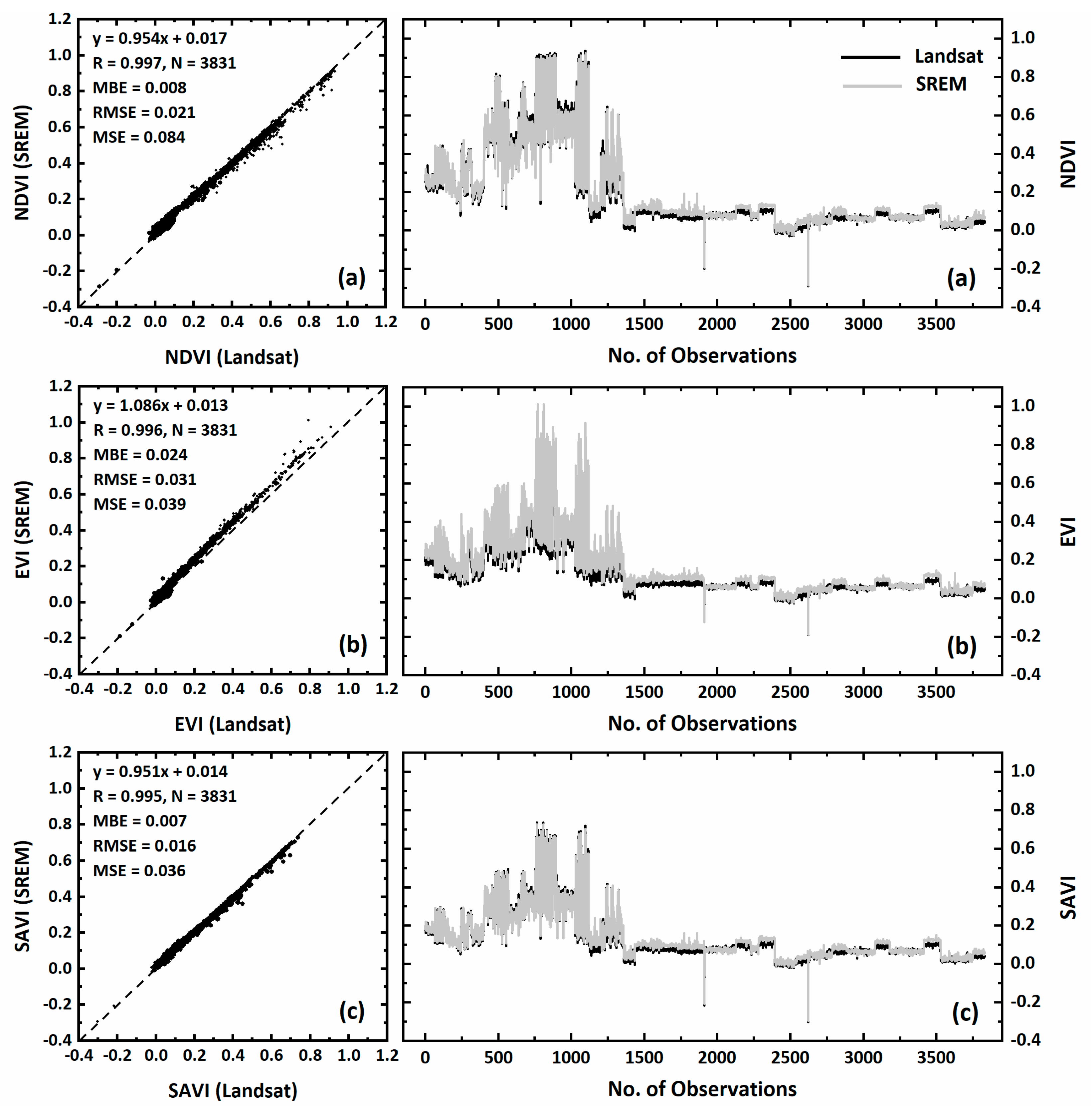
4.5. Application of SREM to Derive Vegetation Indices

Vegetation indices such as NDVI, EVI, and SAVI data are computed using SREM and compared with Landsat vegetation indices (Figure 7) for the urban (2013–2018), vegetated (2013–2018), and desert sites (2000–2018), in order to test the suitability of the SREM data for vegetation and crop monitoring. Results reveal high consistency in the SREM computed vegetation indices NDVI (Figure 7a), EVI (Figure 7b), and SAVI (Figure 7c) compared to Landsat, as most of the observations are found close to the 1:1 line (dotted line) with slope from 0.951 to 1.086, intercept from 0.013 and 0.017, Pearson’s correlation from 0.995 to 0.997, and MBE from 0.007 to 0.024. This comparison is worthy, as an error in the surface reflectance can introduce error in the indices and their potential applications. For example, the SREM SR slightly overestimates in the blue band compared to Landsat, which leads to a larger MBE (0.024) and slopes in the SREM EVI (which uses blue, red, and NIR bands) compared to the NDVI and SAVI, which do not incorporate the blue band. These results show that the SREM SR product is faithful and reliable and can be used for vegetation mapping and monitoring on a global scale.

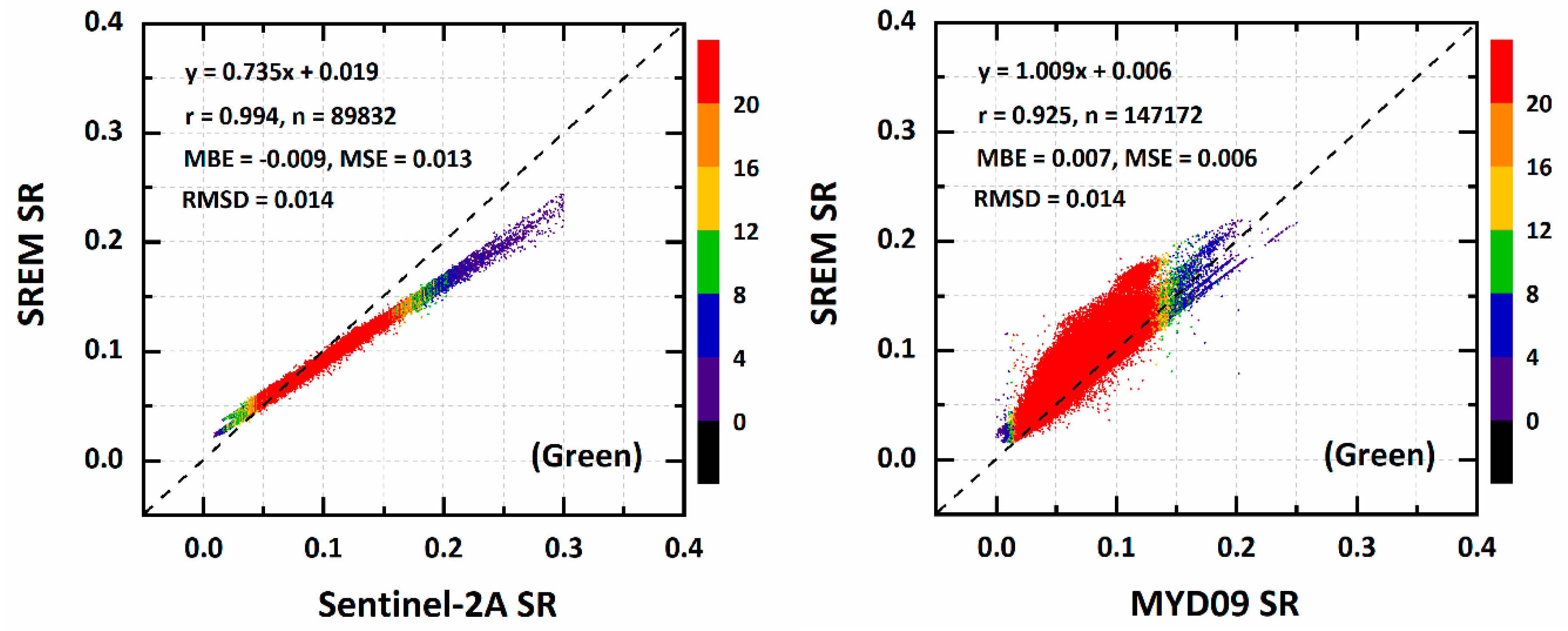
4.6. SREM Implementation in Sentinel-2A and MODIS Data

To further substantiate the applicability of the SREM, preliminary analyses are conducted by SREM using Sentinel-2A and Aqua-MODIS data for Beijing, a city with mixed bright urban surfaces and under effects of severe air pollution episodes. The SREM is applied to cloud-free green band images of Sentinel-2A at 10 m spatial resolution from 8 January to 18 May, 2017, and MODIS at 500 m spatial resolution for the year 2014 (Figure 8). For comparison purposes, the Sentinel-2A SR images are processed using the latest version 2.5.5 of the Sen2Cor atmospheric correction processor, and the Aqua-MODIS Level 2 surface reflectance swath product (MYD09) is used. Figure 8 indicates that most of the scatter points are on or close to the 1:1 line with a high value of r from 0.925 (MODIS) to 0.994 (Sentinel-2A) and small values of MBE from −0.009 (Sentinel-2A) to 0.007 (MODIS) and RMSD of 0.014 for both. The slope between SREM and Sentinel-2A is less than the slope observed for SREM vs. MODIS due to “under-correction “of the Sentinel-2A SR data by the atmospheric correction algorithm, i.e., Sentinel-2A SR values are greater than TOA reflectance over bright surfaces, whereas, SREM SR values are less than TOA reflectance over these surfaces (Figure S2). Overall, these preliminary results suggest that the SREM has the potential to estimate SR also for other multispectral satellite data.

5. Conclusions

The prime objective of this study was to develop a new Simplified and Robust Surface Reflectance Estimation Method (SREM) based on the Satellite Signal in the Solar Spectrum (6SV) radiative transfer (RT) model equations, without integrating information on aerosol particles and atmospheric gases. The SREM surface reflectance (SR) retrievals were validated against in situ measurements collected by an Analytical Spectral Devices (ASD) spectrometer, and cross-compared with Landsat (LEDAPS and LaSRC) SR products for diverse land surfaces and varying atmospheric conditions, as well as tested on Sentinel2A and MODIS data products. This study concluded that the SREM is capable of accurately estimating spectral surface reflectance (SR) without incorporating information on aerosol particles and atmospheric parameters, and the SR retrievals are comparable with the SR data collected by the ASD spectrometer as well as those provided by Landsat SR products (LEDAPS and LaSRC) which use the 6SV model. Larger positive values of MBE were observed for coastal aerosol band compared to longer wavelengths, which may be related to increase scattering effects at lower wavelengths. Large negative values of MBE were observed in SREM from green to SWIR2 bands when compared to Landsat, which were mainly due to “under-correction (lack of atmospheric correction)” of data by the Landsat atmospheric correction algorithms when compared to TOA reflectance. The preliminary analysis implies that SREM has a strong potential for augmenting vegetation and crop monitoring and it can be implemented with Sentinel-2A and MODIS data or other multispectral satellite data sets.

References

1. Huete, A.; Didan, K.; Miura, T.; Rodriguez, E.; Gao, X.; Ferreira, L. Overview of the radiometric and biophysical performance of the MODIS vegetation indices. Remote Sens. Environ. 2002, 83, 195–213. [Google Scholar] [CrossRef]
2. Peng, G.; Ruiliang, P.; Biging, G.S.; Larrieu, M.R. Estimation of forest leaf area index using vegetation indices derived from hyperion hyperspectral data. IEEE Trans. Geosci. Remote. Sens. 2003, 41, 1355–1362. [Google Scholar] [CrossRef] [Green Version]
3. Zhang, R.; Qu, J.J.; Liu, Y.; Hao, X.; Huang, C.; Zhan, X. Detection of burned areas from mega-fires using daily and historical MODIS surface reflectance. Int. J. Remote Sens. 2015, 36, 1167–1187. [Google Scholar]
4. Friedl, M.A.; Sulla-Menashe, D.; Tan, B.; Schneider, A.; Ramankutty, N.; Sibley, A.; Huang, X. MODIS Collection 5 global land cover: Algorithm refinements and characterization of new datasets. Remote Sens. Environ. 2010, 114, 168–182. [Google Scholar] [CrossRef]
5. Bilal, M.; Nichol, J.E. Evaluation of MODIS aerosol retrieval algorithms over the Beijing-Tianjin-Hebei region during low to very high pollution events. J. Geophys. Res. Atmos. 2015, 120, 7941–7957. [Google Scholar] [CrossRef]
6. Bilal, M.; Nichol, J.E.; Chan, P.W. Validation and accuracy assessment of a Simplified Aerosol Retrieval Algorithm (SARA) over Beijing under low and high aerosol loadings and dust storms. Remote Sens. Environ. 2014, 153, 50–60. [Google Scholar] [CrossRef]
7. Bilal, M.; Nichol, J.E.; Bleiweiss, M.P.; Dubois, D. A Simplified high resolution MODIS Aerosol Retrieval Algorithm (SARA) for use over mixed surfaces. Remote Sens. Environ. 2013, 136, 135–145. [Google Scholar] [CrossRef]
8. Nazeer, M.; Wong, M.S.; Nichol, J.E. A new approach for the estimation of phytoplankton cell counts associated with algal blooms. Sci. Total Environ. 2017, 590, 125–138. [Google Scholar] [CrossRef] [PubMed]
9. Chavez, P.S. An improved dark-object subtraction technique for atmospheric scattering correction of multispectral data. Remote Sens. Environ. 1988, 24, 459–479. [Google Scholar] [CrossRef]
10. Smith, G.M.; Milton, E.J. The use of the empirical line method to calibrate remotely sensed data to reflectance. Int. J. Remote Sens. 1999, 20, 2653–2662. [Google Scholar] [CrossRef]
11. Richter, R. A spatially adaptive fast atmospheric correction algorithm. Int. J. Remote Sens. 1996, 17, 1201–1214. [Google Scholar] [CrossRef]
12. Nazeer, M.; Nichol, J.E.; Yung, Y.K. Evaluation of atmospheric correction models and Landsat surface reflectance product in an urban coastal environment. Int. J. Remote Sens. 2014, 35, 6271–6291. [Google Scholar] [CrossRef]
13. Matthew, M.W.; Adler-Golden, S.M.; Berk, A.; Richtsmeier, S.C.; Levine, R.Y.; Bernstein, L.S.; Acharya, P.K.; Anderson, G.P.; Felde, G.W.; Hoke, M.L.; et al. Status of atmospheric correction using a MODTRAN4-based algorithm. In Algorithms for Multispectral, Hyperspectral, and Ultraspectral Imagery VI; International Society for Optics and Photonics: Bellingham, WA, USA, 2000; Volume 4049, p. 199. [Google Scholar]
14. Sterckx, S.; Knaeps, E.; Adriaensen, S.; Reusen, I.; De Keukelaere, L.; Hunter, P.; Giardino, C.; Odermatt, D. OPERA: An atmospheric correction for land and water. In Proceedings of the Sentinel-3 for Science Workshop, Venice, Italy, 2–5 June 2015. [Google Scholar]
15. Frantz, D.; Roder, A.; Stellmes, M.; Hill, J. An operational radiometric landsat preprocessing framework for large-area time series applications. IEEE Trans. Geosci. Remote. Sens. 2016, 54, 3928–3943. [Google Scholar] [CrossRef]
16. Masek, J.G.; Vermote, E.F.; Saleous, N.E.; Wolfe, R.; Hall, F.G.; Huemmrich, K.F.; Gao, F.; Kutler, J.; Lim, T.-K. A Landsat surface reflectance dataset for North America, 1990-2000—IEEE Xplore Document. IEEE Geosci. Remote Sens. Lett. 2006, 3, 68–72. [Google Scholar] [CrossRef]
17. Vermote, E.; Justice, C.; Claverie, M.; Franch, B. Preliminary analysis of the performance of the Landsat 8/OLI land surface reflectance product. Remote Sens. Environ. 2016, 185, 46–56. [Google Scholar] [CrossRef]
18. Berk, A.; Bernstein, L.S.; Robertson, D.C. MODTRAN: A Moderate Resolution Model for LOWTRAN 7; Spectral Sciences Inc.: Burlington, MA, USA, 1989. [Google Scholar]
19. Tanré, D.; Deroo, C.; Duhaut, P.; Herman, M.; Morcrette, J.J.; Perbos, J.; Deschamps, P.Y. Description of a computer code to simulate the satellite signal in the solar spectrum: The 5S code. Int. J. Remote Sens. 1990, 11, 659–668. [Google Scholar] [CrossRef]
20. Vermote, E.F.; Tanre, D.; Deuze, J.L.; Herman, M.; Morcette, J.-J. Second simulation of the satellite signal in the solar spectrum, 6S: An overview. IEEE Trans. Geosci. Remote. Sens. 1997, 35, 675–686. [Google Scholar] [CrossRef]
21. Wilson, R.T. Py6S: A Python interface to the 6S radiative transfer model. Comput. Geosci. 2013, 51, 166. [Google Scholar] [CrossRef]
22. Kotchenova, S.Y.; Vermote, E.F.; Levy, R.; Lyapustin, A. Radiative transfer codes for atmospheric correction and aerosol retrieval: Intercomparison study. Appl. Opt. 2008, 47, 2215. [Google Scholar] [CrossRef]
23. Wilson, R.T.; Milton, E.J.; Nield, J.M. Are visibility-derived AOT estimates suitable for parameterizing satellite data atmospheric correction algorithms? Int. J. Remote Sens. 2015, 36, 1675–1688. [Google Scholar] [CrossRef] [Green Version]
24. Nguyen, H.; Jung, J.; Lee, J.; Choi, S.-U.; Hong, S.-Y.; Heo, J.; Nguyen, H.C.; Jung, J.; Lee, J.; Choi, S.-U.; et al. Optimal atmospheric correction for above-ground forest biomass estimation with the ETM+ remote sensor. Sensors 2015, 15, 18865–18886. [Google Scholar] [CrossRef]
25. López-Serrano, P.; Corral-Rivas, J.; Díaz-Varela, R.; Álvarez-González, J.; López-Sánchez, C. Evaluation of radiometric and atmospheric correction algorithms for aboveground forest biomass estimation using Landsat 5 TM data. Remote Sens. 2016, 8, 369. [Google Scholar] [CrossRef]
26. Lolli, S.; Alparone, L.; Garzelli, A.; Vivone, G. Haze correction for contrast-based multispectral pansharpening. IEEE Geosci. Remote. Sens. Lett. 2017, 14, 2255–2259. [Google Scholar] [CrossRef]
27. Doxani, G.; Vermote, E.; Roger, J.-C.; Gascon, F.; Adriaensen, S.; Frantz, D.; Hagolle, O.; Hollstein, A.; Kirches, G.; Li, F.; et al. Atmospheric correction inter-comparison exercise. Remote Sens. 2018, 10, 352. [Google Scholar] [CrossRef]
28. Justice, C.; Townshend, J.R.; Vermote, E.; Masuoka, E.; Wolfe, R.; Saleous, N.; Roy, D.; Morisette, J. An overview of MODIS Land data processing and product status. Remote Sens. Environ. 2002, 83, 3–15. [Google Scholar] [CrossRef]
29. Vermote, E.; Justice, C.; Csiszar, I. Early evaluation of the VIIRS calibration, cloud mask and surface reflectance Earth data records. Remote Sens. Environ. 2014, 148, 134–145. [Google Scholar] [CrossRef] [Green Version]
30. Muller-Wilm, U.; Louis, J.; Richter, R.; Gascon, F.; Niezette, M. Sentinel-2 Level 2A prototype processor: Architecture, algorithms and first results. In Proceedings of the ESA Living Planet Symposium, Edinburgh, UK, 9–13 September 2013. [Google Scholar]
31. Claverie, M.; Ju, J.; Masek, J.G.; Dungan, J.L.; Vermote, E.F.; Roger, J.C.; Skakun, S.V.; Justice, C. The Harmonized Landsat and Sentinel-2 surface reflectance data set. Remote Sens. Environ. 2018, 219, 145–161. [Google Scholar] [CrossRef]
32. Claverie, M.; Vermote, E.F.; Franch, B.; Masek, J.G. Evaluation of the Landsat-5 TM and Landsat-7 ETM + surface reflectance products. Remote Sens. Environ. 2015, 169, 390–403. [Google Scholar] [CrossRef]
33. Gascon, F.; Bouzinac, C.; Thépaut, O.; Jung, M.; Francesconi, B.; Louis, J.; Lonjou, V.; Lafrance, B.; Massera, S.; Gaudel-Vacaresse, A.; et al. Copernicus Sentinel-2A Calibration and products validation status. Remote Sens. 2017, 9, 584. [Google Scholar] [CrossRef]
34. Li, Y.; Chen, J.; Ma, Q.; Zhang, H.K.; Liu, J. Evaluation of Sentinel-2A surface reflectance derived using Sen2Cor in North America. IEEE J. Sel. Top. Appl. Earth Obs. Remote. Sens. 2018, 11, 1997–2021. [Google Scholar] [CrossRef]
35. Maiersperger, T.K.; Scaramuzza, P.L.; Leigh, L.; Shrestha, S.; Gallo, K.P.; Jenkerson, C.B.; Dwyer, J.L. Characterizing LEDAPS surface reflectance products by comparisons with AERONET, field spectrometer, and MODIS data. Remote Sens. Environ. 2013, 136, 1–13. [Google Scholar] [CrossRef] [Green Version]
36. Vuolo, F.; Żółtak, M.; Pipitone, C.; Zappa, L.; Wenng, H.; Immitzer, M.; Weiss, M.; Baret, F.; Atzberger, C. Data service platform for Sentinel-2 surface reflectance and value-added products: System use and examples. Remote Sens. 2016, 8, 938. [Google Scholar] [CrossRef]
37. Vuolo, F.; Mattiuzzi, M.; Atzberger, C. Comparison of the Landsat Surface Reflectance Climate Data Record (CDR) and manually atmospherically corrected data in a semi-arid European study area. Int. J. Appl. Earth Obs. Geoinf. 2015, 41, 1–10. [Google Scholar] [CrossRef]
38. Choi, M.; Kim, J.; Lee, J.; Kim, M.; Park, Y.-J.; Holben, B.; Eck, T.F.; Li, Z.; Song, H.H. GOCI Yonsei aerosol retrieval version 2 products: An improved algorithm and error analysis with uncertainty estimation from 5-year validation over East Asia. Atmos. Meas. Tech. 2018, 11, 385–408. [Google Scholar] [CrossRef]
39. Bilal, M.; Nichol, J.; Wang, L. New customized methods for improvement of the MODIS C6 Dark Target and Deep Blue merged aerosol product. Remote Sens. Environ. 2017, 197, 115–124. [Google Scholar] [CrossRef]
40. Bilal, M.; Nichol, J. Evaluation of the NDVI-based pixel selection criteria of the MODIS C6 Dark Target and Deep Blue combined aerosol product. IEEE J. Sel. Top. Appl. Earth Obs. Remote Sens. 2017, 10, 3448–3453. [Google Scholar] [CrossRef]
41. Sulla-Menashe, D.; Gray, J.M.; Abercrombie, S.P.; Friedl, M.A. Hierarchical mapping of annual global land cover 2001 to present: The MODIS Collection 6 Land Cover product. Remote Sens. Environ. 2019, 222, 183–194. [Google Scholar] [CrossRef]
42. Kotchenova, S.Y.; Vermote, E.F.; Matarrese, R.; Frank, J.; Klemm, J. Validation of a vector version of the 6S radiative transfer code for atmospheric correction of satellite data. Part I: Path radiance. Appl. Opt. 2006, 45, 6762–6774. [Google Scholar] [CrossRef]
43. LISE. OLCI Level 2: Rayleigh Correction Over Land (S3-L2-SD-03-C15-LISE-ATBD). Available online: https://sentinels.copernicus.eu/documents/247904/349589/OLCI_L2_Rayleigh_Correction_Land.pdf (accessed on 17 October 2018).
44. Hansen, J.E.; Travis, L.D. Light scattering in planetary atmospheres. Space Sci. Rev. 1974, 16, 527–610. [Google Scholar] [CrossRef]
45. Tanre, D.; Herman, M.; Deschamps, P.Y.; de Leffe, A. Atmospheric modeling for space measurements of ground reflectances, including bidirectional properties. Appl. Opt. 1979, 18, 3587–3594. [Google Scholar] [CrossRef]
46. Liu, C.-H.; Liu, G.-R. Aerosol optical depth retrieval for spot HRV images. J. Mar. Sci. Technol. 2009, 17, 300–305. [Google Scholar]
47. Roy, D.P.; Qin, Y.; Kovalskyy, V.; Vermote, E.F.; Ju, J.; Egorov, A.; Hansen, M.C.; Kommareddy, I.; Yan, L. Conterminous United States demonstration and characterization of MODIS-based Landsat ETM+ atmospheric correction. Remote Sens. Environ. 2014, 140, 433–449. [Google Scholar] [CrossRef]
48. Ju, J.; Roy, D.P.; Vermote, E.; Masek, J.; Kovalskyy, V. Continental-scale validation of MODIS-based and LEDAPS Landsat ETM+ atmospheric correction methods. Remote Sens. Environ. 2012, 122, 175–184. [Google Scholar] [CrossRef] [Green Version]
49. Roy, D.P.; Ju, J.; Kline, K.; Scaramuzza, P.L.; Kovalskyy, V.; Hansen, M.; Loveland, T.R.; Vermote, E.; Zhang, C. Web-enabled Landsat Data (WELD): Landsat ETM+ composited mosaics of the conterminous United States. Remote Sens. Environ. 2010, 114, 35–49. [Google Scholar] [CrossRef]
50. Markham, B.L.; Helder, D.L. Forty-year calibrated record of earth-reflected radiance from Landsat: A review. Remote Sens. Environ. 2012, 122, 30–40. [Google Scholar] [CrossRef] [Green Version]
51. Schaepman-Strub, G.; Schaepman, M.E.; Painter, T.H.; Dangel, S.; Martonchik, J.V. Reflectance quantities in optical remote sensing—Definitions and case studies. Remote Sens. Environ. 2006, 103, 27–42. [Google Scholar] [CrossRef]
52. Rouse, J.; Haas, R.; Schell, J.; Deering, D. Monitoring vegetation systems in the great plains with ERTS. In Proceedings of the Third ERTS Symposium, NASA, Washington, DC, USA, 10–14 December 1973; pp. 309–317. [Google Scholar]
53. Berterretche, M.; Hudak, A.T.; Cohen, W.B.; Maiersperger, T.K.; Gower, S.T.; Dungan, J. Comparison of regression and geostatistical methods for mapping Leaf Area Index (LAI) with Landsat ETM+ data over a boreal forest. Remote Sens. Environ. 2005, 96, 49–61. [Google Scholar] [CrossRef] [Green Version]
54. Curran, P.; Hay, A. The importance of measurement error for certain procedures in remote sensing at optical wavelengths. Photogramm. Eng. Remote Sens. 1986, 52, 229–241. [Google Scholar]
55. Martins, V.S.; Soares, J.V.; Novo, E.M.L.M.; Barbosa, C.C.F.; Pinto, C.T.; Arcanjo, J.S.; Kaleita, A. Continental-scale surface reflectance product from CBERS-4 MUX data: Assessment of atmospheric correction method using coincident Landsat observations. Remote Sens. Environ. 2018, 218, 55–68. [Google Scholar] [CrossRef]
Figure 1. Sites used for validation and comparison of SREM derived surface reflectance (SR) products for Landsat and Sentinel-2A. Please refer to the “S/N” in Table 2 for labeled values, and WRS-2 (Worldwide Reference System) path/row numbers.
Remotesensing 11 01344 g001
Figure 2. Systematic methodology of the SREM (Simplified and Robust Surface Reflectance Estimation Method).
Remotesensing 11 01344 g002
Figure 3. Cross-comparison between coincident SREM and Landsat (LEDAPS and LaSRC) SR retrievals over urban and vegetated sites from 2013–2018, and desert (arid) sites from 2013–2018. Where, coastal aerosol band = (a) urban sites, (b) vegetated sites, and (c) desert sites; blue band = (d) urban sites, (e) vegetated sites, and (f) desert sites; green band = (g) urban sites, (h) vegetated sites, and (i) desert sites; red band = (j) urban sites, (k) vegetated sites, and (l) desert sites; NIR = (m) urban sites, (n) vegetated sites, and (o) desert sites; SWIR1 = (p) urban sites, (q) vegetated sites, and (r) desert sites; SWIR2 = (s) urban sites, (t) vegetated sites, and (u) desert sites; the black line = Landsat retrievals; the grey line = SREM retrievals; and the dashed line = 1:1 line.
Remotesensing 11 01344 g003
Figure 4. Cross-comparison between coincident Landsat (LaSRC) and SREM SR retrievals over AERONET sites for low to high AOD levels from 2013 to 2018. The dashed line is the 1:1 line.
Remotesensing 11 01344 g004
Figure 5. Spatial comparison between LaSRC (left image in each panel) and SREM (right image in each panel) corrected images for different path/rows including (a) 122/44, (b) 170/78, (c) 201/32, (d) 199/26, (e) 15/33 and (f) 25/39. All images are composed using the "natural looking" false color composite of 654 as RGB. All images are North up. No stretch/contrast is applied to the images.
Remotesensing 11 01344 g005
Figure 6. Cross-comparison between SREM and LaSRC data for six paths/rows located in Asia (122/44), Africa (170/78), Europe (119/26 and 201/32), and the United States of America (15/33 and 25/39) from 2013 to 2018 for a large variety of surface types under varying atmospheric conditions. The dashed line is the 1:1 line and the color bar represents the relative frequency of the coincident points.
Remotesensing 11 01344 g006
Figure 7. Cross-comparison of NDVI (a), EVI (b), and SAVI (c) data based on the SREM and Landsat (LEDAPS and LaSRC) SR products from 2000 to 2018 for the 35 selected urban, vegetated, and desert sites. The dashed line is the 1:1 line; the grey line = SREM retrievals; the black line = Landsat retrievals which are partially hidden by SREM.
Remotesensing 11 01344 g007
Figure 8. Cross-comparison of SREM vs. Sen2Cor 2.5.5, and SREM vs. MYD09 for the Beijing site. Cloud-free images of Sentinel-2A at 10 m spatial resolution from 8 January to 18 May, 2017, and MODIS at 500 m spatial resolution for the year 2014 are used for cross-comparison. The dashed line represents the 1:1 (y = x) line and the color bar represent the relative frequency of the coincident points.
Remotesensing 11 01344 g008