Quantifying Canopy Tree Loss and Gap Recovery in Tropical Forests under Low-Intensity Logging Using VHR Satellite Imagery and Airborne LiDAR

 , ,
, ,
Abstract
:
1. Introduction
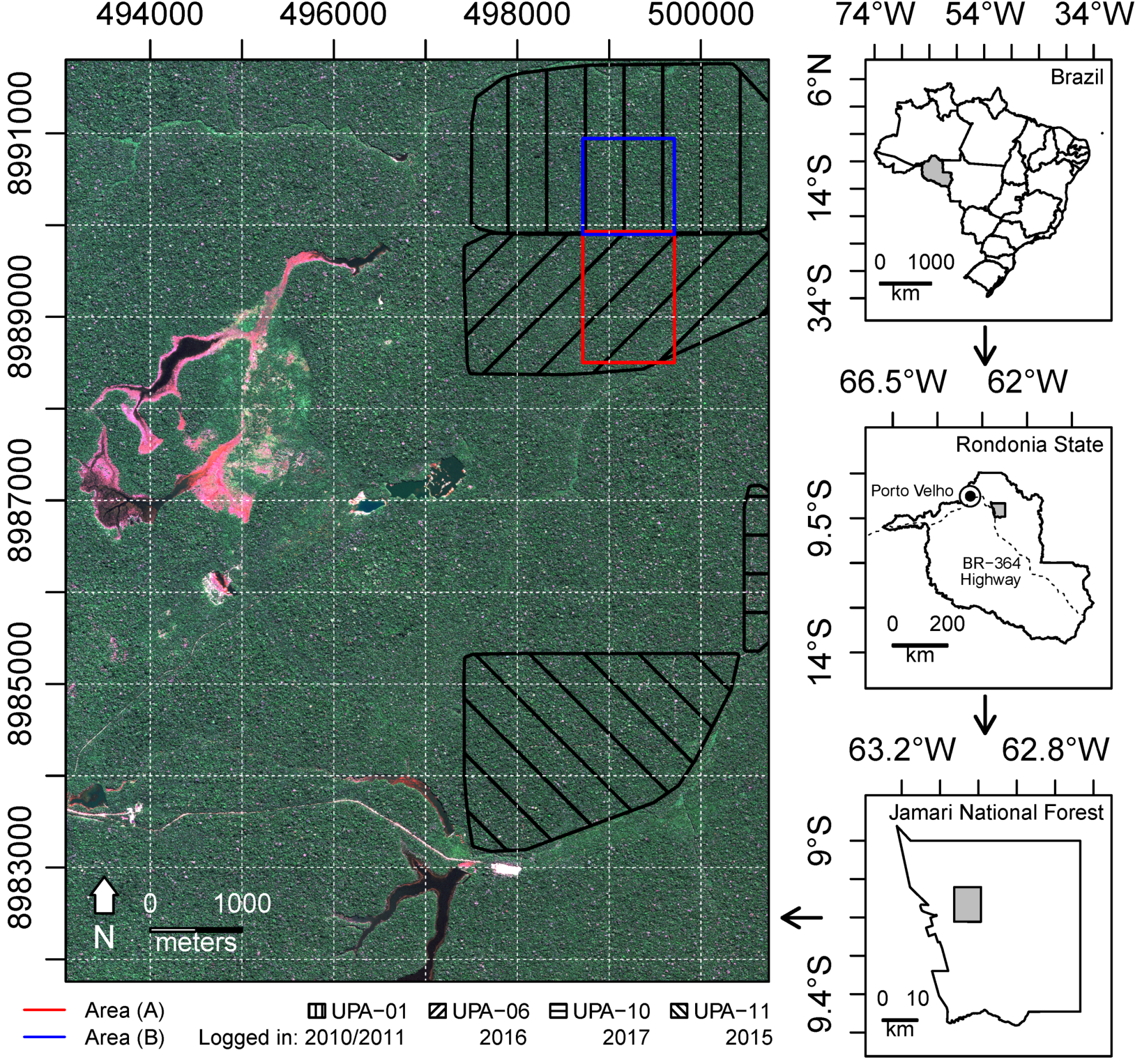
2. Study Area
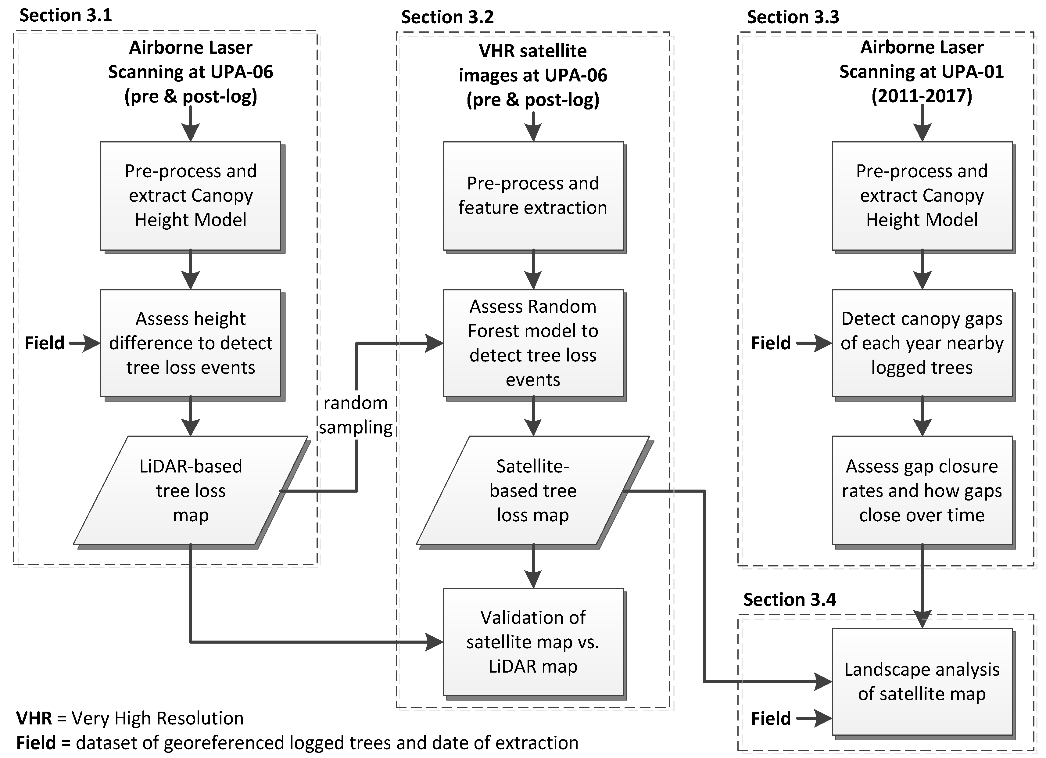
3. Material and Methods
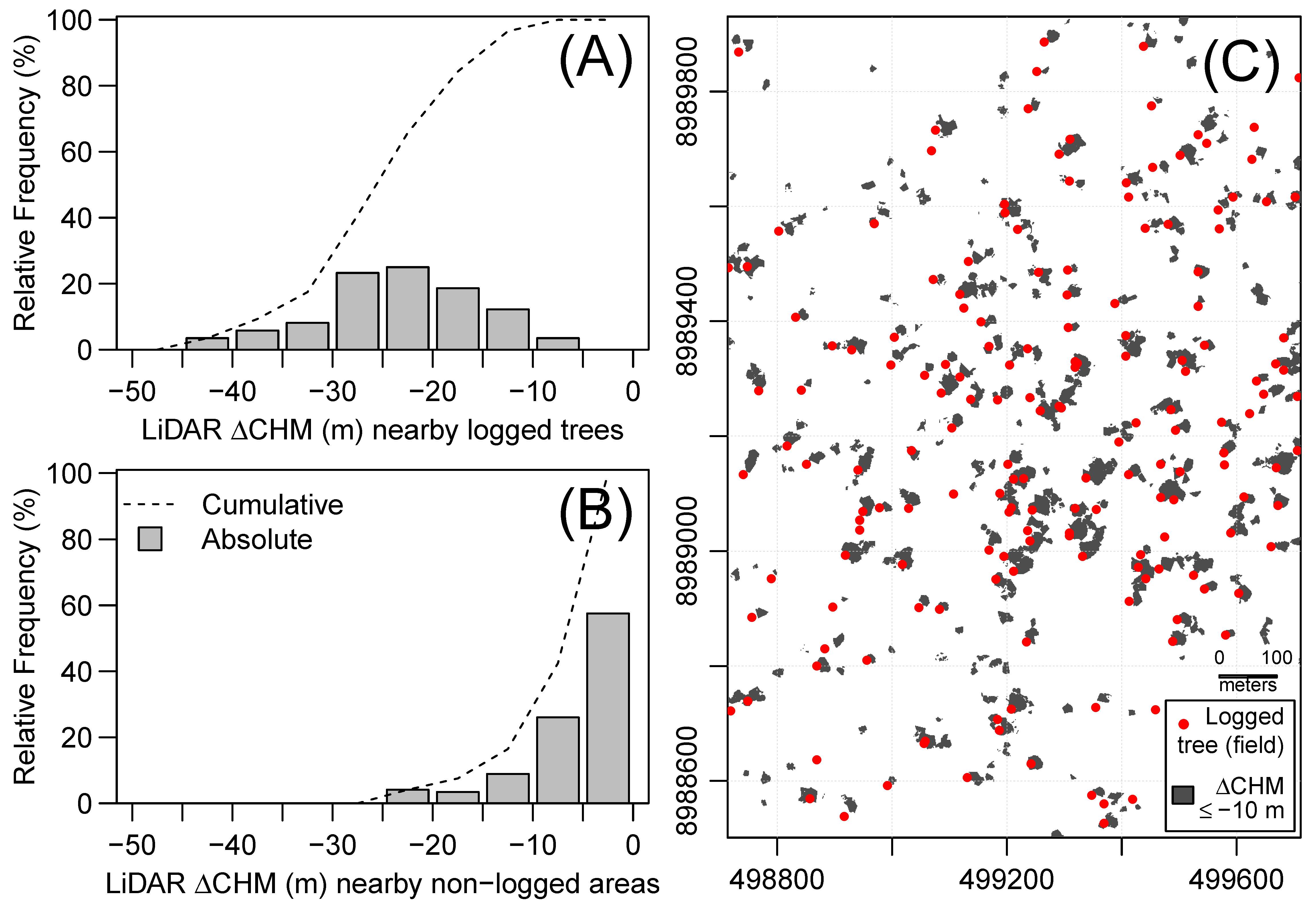
3.1. Tree Loss Detection Using LiDAR Data
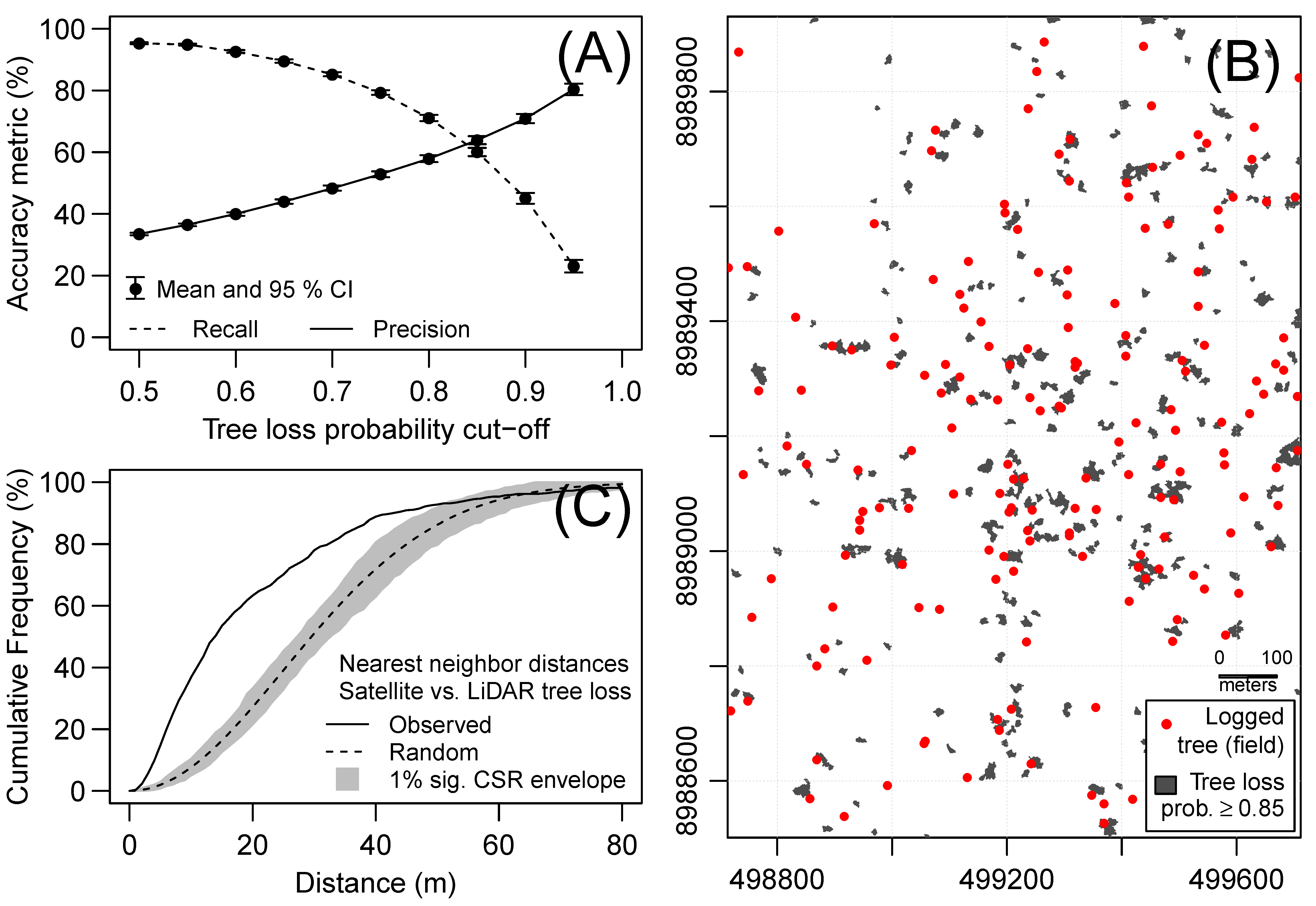
3.2. Tree Loss Detection Using VHR Satellite Data and RF Model
3.2.1. Satellite Data Acquisition and Preprocessing
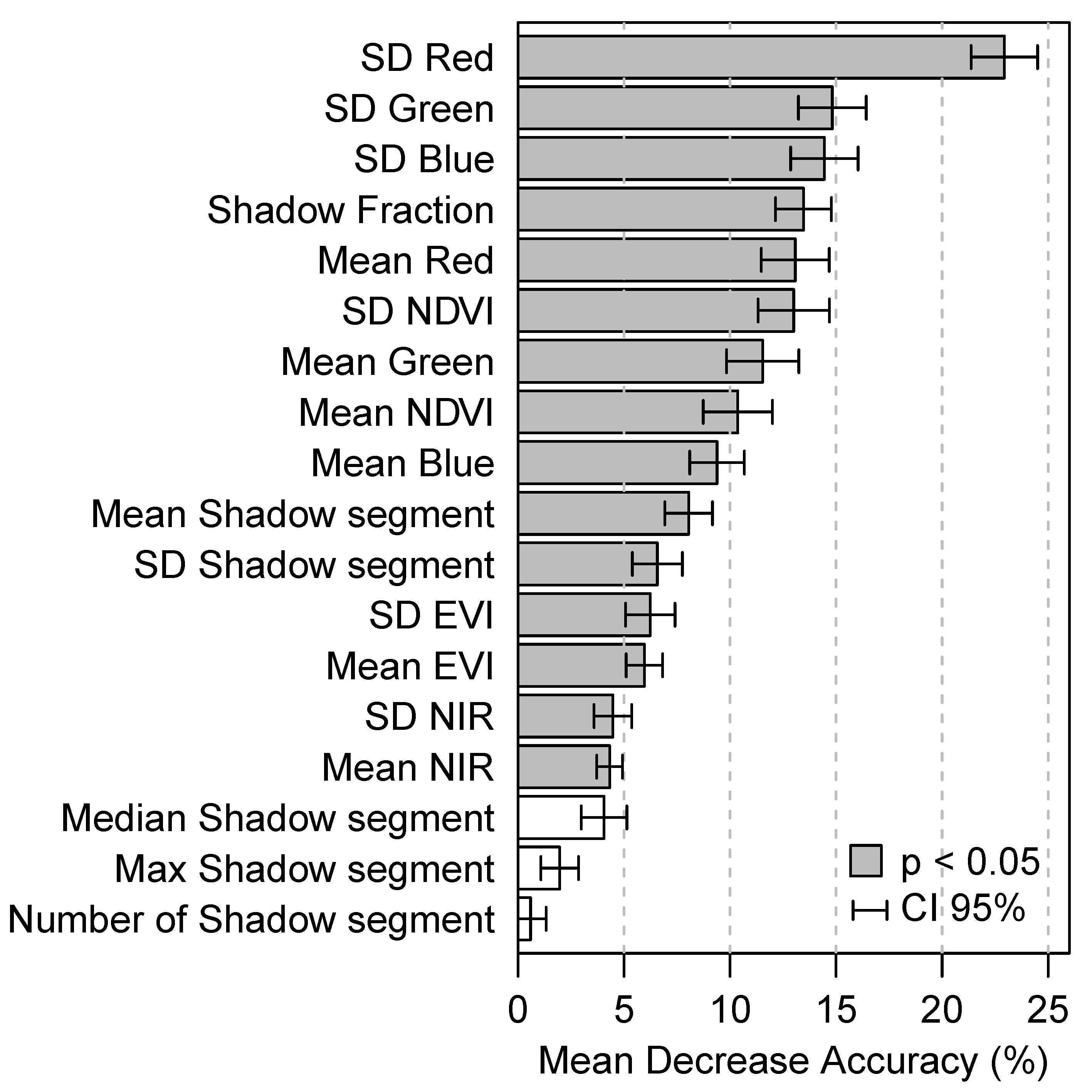
3.2.2. Selection and Extraction of VHR Satellite Metrics
3.2.3. RF Model
3.2.4. Validation of the Satellite-Based Tree Loss Map
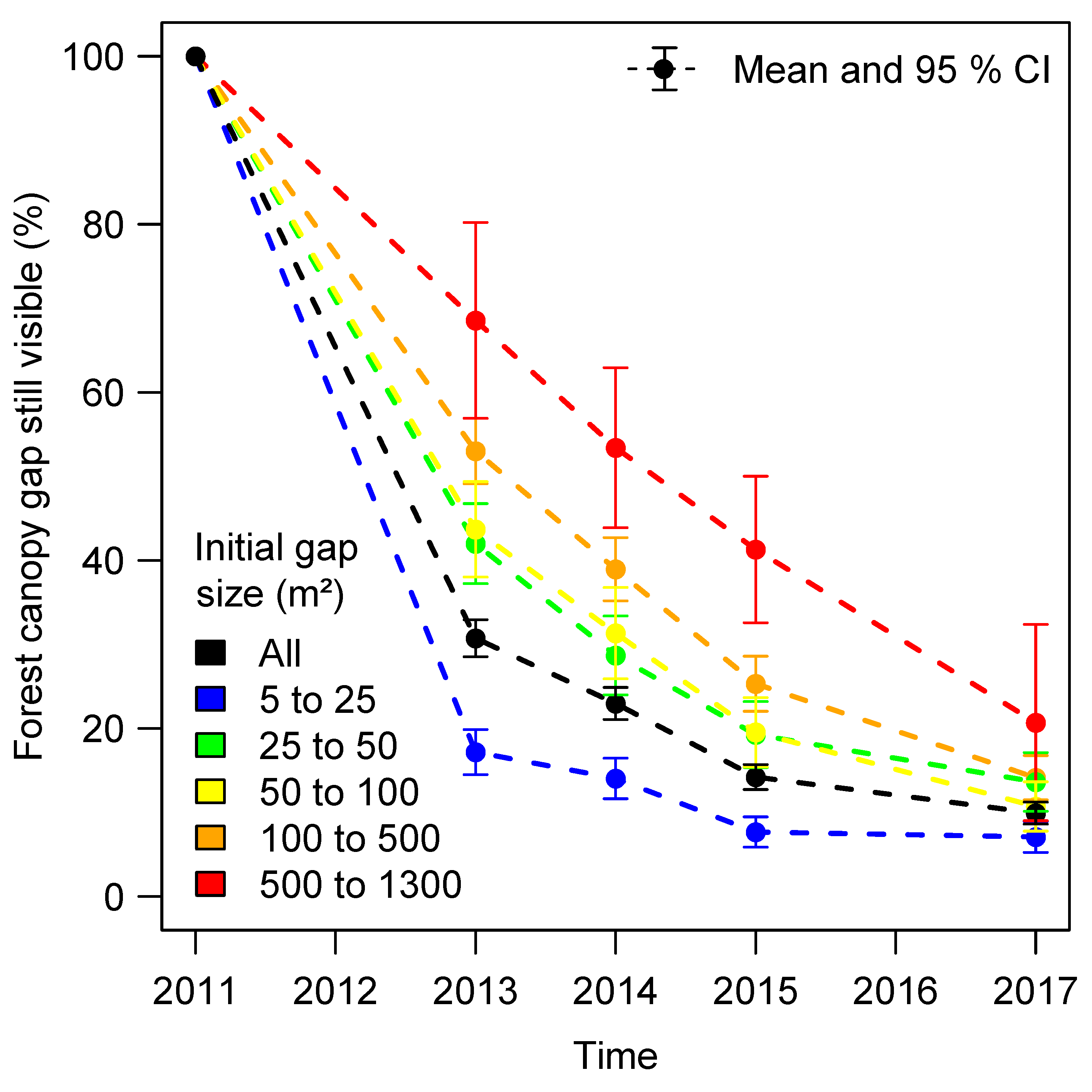
3.3. Assessment of Tree-Fall Gaps Recovery Using LiDAR Data
3.4. Landscape Analysis of Satellite-Based Tree Loss Map
4. Results
4.1. Detecting Tree Loss Events Using LiDAR Data
4.2. Detecting Tree Loss Events Using VHR Satellite Data and RF Model
4.3. Tree-Fall Gap Recovery Assessment Using LiDAR Data
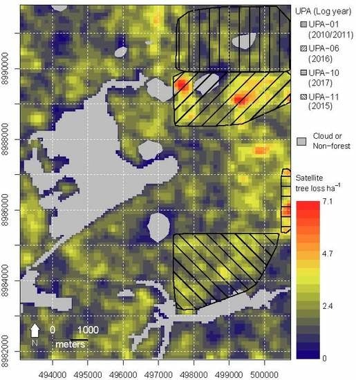
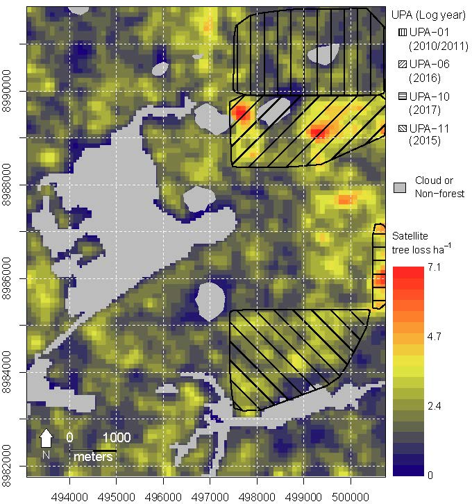
4.4. Landscape Analysis of Satellite-Based Tree Loss Map
5. Discussion
6. Conclusions
Supplementary Materials
Author Contributions
Funding
Acknowledgments
Conflicts of Interest
References
- Contreras-Hermosilla, A.; Doornbosch, R.; Lodge, M. The Economics of Illegal Logging and Associated Trade. Round Table Sustain. Dev. 2007, 33, 8–9. [Google Scholar]
- Lawson, S.; Macfaul, L. Illegal Logging and Related Trade: Indicators of the Global Response; Chatham House Rep. 132 + xix; Chatham House: London, UK, 2010. [Google Scholar]
- Asner, G.P.; Knapp, D.E.; Broadbent, E.N.; Oliveira, P.J.C.; Keller, M.; Silva, J.N. Selective Logging in the Brazilian Amazon. Science 2005, 310, 480–482. [Google Scholar] [CrossRef] [PubMed]
- Aragão, L.E.O.C.; Poulter, B.; Barlow, J.B.; Anderson, L.O.; Malhi, Y.; Saatchi, S.; Phillips, O.L.; Gloor, E. Environmental change and the carbon balance of Amazonian forests. Biol. Rev. 2014, 89, 913–931. [Google Scholar] [CrossRef] [PubMed]
- Cochrane, M.A. Fire science for rainforests. Nature 2003, 421, 913–919. [Google Scholar] [CrossRef]
- LaManna, J.A.; Martin, T.E. Logging impacts on avian species richness and composition differ across latitudes and foraging and breeding habitat preferences. Biol. Rev. 2017, 92, 1657–1674. [Google Scholar] [CrossRef] [PubMed]
- Osazuwa-Peters, O.L.; Jiménez, I.; Oberle, B.; Chapman, C.A.; Zanne, A.E. Selective logging: Do rates of forest turnover in stems, species composition and functional traits decrease with time since disturbance? A 45 year perspective. For. Ecol. Manag. 2015, 357, 10–21. [Google Scholar] [CrossRef]
- Buchanan, G.M.; Beresford, A.E.; Hebblewhite, M.; Escobedo, F.J.; De Klerk, H.M.; Donald, P.F.; Escribano, P.; Koh, L.; Martínez-López, J.; Pettorelli, N.; et al. Free satellite data key to conservation. Science 2018, 361, 139–140. [Google Scholar]
- Stone, T.A.; Lefebvre, P. Using multi-temporal satellite data to evaluate selective logging in Pará, Brazil. Int. J. Remote Sens. 1998, 19, 2517–2526. [Google Scholar] [CrossRef]
- Wang, Y.; Ziv, G.; Adami, M.; Mitchard, E.; Batterman, S.A.; Buermann, W.; Schwantes, B.; Hur, B.; Junior, M.; Matias, S.; et al. Mapping tropical disturbed forests using multi-decadal 30 m optical satellite imagery. Remote Sens. Environ. 2019, 221, 474–488. [Google Scholar] [CrossRef]
- Read, J.M.; Clark, D.B.; Venticinque, E.M.; Moreira, M.P. Application of merged 1-m and 4-m resolution satellite data to research and management in tropical forests. J. Appl. Ecol. 2003, 40, 592–600. [Google Scholar] [CrossRef]
- Clark, D.B.; Castro, C.S.; Alvarado, L.D.A.; Read, J.M. Quantifying mortality of tropical rain forest trees using high-spatial-resolution satellite data. Ecol. Lett. 2004, 7, 52–59. [Google Scholar] [CrossRef]
- Clark, D.B.; Read, J.M.; Clark, M.L.; Cruz, A.M.; Dotti, M.F.; Clark, D.A. Application of 1-m and 4-m resolution satellite data to ecological studies of tropical rain forests. Ecol. Appl. 2004, 14, 61–74. [Google Scholar] [CrossRef]
- Kellner, J.R.; Hubbell, S.P. Adult mortality in a low-density tree population using high-resolution remote sensing. Ecology 2017, 98, 1700–1709. [Google Scholar] [CrossRef] [PubMed]
- Wulder, M.A.; White, J.C.; Coops, N.C.; Butson, C.R. Multi-temporal analysis of high spatial resolution imagery for disturbance monitoring. Remote Sens. Environ. 2008, 112, 2729–2740. [Google Scholar] [CrossRef]
- Guo, Q.; Kelly, M.; Gong, P.; Liu, D. An Object-Based Classification Approach in Mapping Tree Mortality Using High Spatial Resolution Imagery. GISci. Remote Sens. 2007, 44, 24–47. [Google Scholar] [CrossRef]
- Asner, G.P.; Powell, G.V.N.; Mascaro, J.; Knapp, D.E.; Clark, J.K.; Jacobson, J.; Kennedy-Bowdoin, T.; Balaji, A.; Paez-Acosta, G.; Victoria, E.; et al. High-resolution forest carbon stocks and emissions in the Amazon. Proc. Natl. Acad. Sci. USA 2010, 107, 16738–16742. [Google Scholar] [CrossRef] [PubMed]
- d’Oliveira, M.V.N.; Reutebuch, S.E.; McGaughey, R.J.; Andersen, H.E. Estimating forest biomass and identifying low-intensity logging areas using airborne scanning lidar in Antimary State Forest, Acre State, Western Brazilian Amazon. Remote Sens. Environ. 2012, 124, 479–491. [Google Scholar] [CrossRef]
- Andersen, H.E.; Reutebuch, S.E.; McGaughey, R.J.; d’Oliveira, M.V.N.; Keller, M. Monitoring selective logging in western amazonia with repeat lidar flights. Remote Sens. Environ. 2014, 151, 157–165. [Google Scholar] [CrossRef]
- Leitold, V.; Morton, D.C.; Longo, M.; dos-Santos, M.N.; Keller, M.; Scaranello, M. El Niño drought increased canopy turnover in Amazon forests. New Phytol. 2018, 219, 959–971. [Google Scholar] [CrossRef]
- IBGE. Mapa Temático-Mapa de Vegetação do Brasil; Brazilian Institute of Geography and Statistics: Rio de Janeiro, Brazil, 2006. [Google Scholar]
- Harris, I.; Jones, P.D.; Osborn, T.J.; Lister, D.H. Updated high-resolution grids of monthly climatic observations—The CRU TS3.10 Dataset. Int. J. Climatol. 2014, 34, 623–642. [Google Scholar] [CrossRef]
- USGS Shuttle Radar Topography Mission, 1 Arc Second, v.2.1; United States Geological Survey: Pasadena, LA, USA, 2006.
- Isenburg, M. LAStools—Efficient Tools for LiDAR Processing v.3.1.1; Rapidlasso: Gilching, Germany, 2018. [Google Scholar]
- McGaughey, R.J. FUSION/LDV: Software for LIDAR Data Analysis and Visualization v. 3.6; United States Department of Agriculture: Seattle, WA, USA, 2016.
- Silva, C.A.; Crookston, N.L.; Hudak, A.T.; Vierling, L.A.; Klauberg, C.; Cardil, A. rLiDAR: LiDAR Data Processing and Visualization v.0.1.1; NASA Goddard Space Flight Center: Greenbelt, ML, USA, 2017.
- Vermote, E.; Tanre, D.; Deuze, J.L.; Herman, M.; Morcrette, J.J. Second Simulation of the Satellite Signal in the Solar Spectrum (6S). 6S User Guide Version 2. Appendix III: Description of the subroutines. IEEE Trans. Geosci. Remote Sens. 1997, 35, 675–686. [Google Scholar] [CrossRef]
- Grizonnet, M.; Michel, J.; Poughon, V.; Inglada, J.; Savinaud, M.; Cresson, R. Orfeo ToolBox: Open source processing of remote sensing images. Open Geospat. Data Softw. Stand. 2017, 2, 15. [Google Scholar] [CrossRef]
- Fasbender, D.; Radoux, J.; Bogaert, P. Bayesian data fusion for adaptable image pansharpening. IEEE Trans. Geosci. Remote Sens. 2008, 46, 1847–1857. [Google Scholar] [CrossRef]
- Leutner, B.; Horning, N.; Schwalb-Willmann, J. RStoolbox: Tools for Remote Sensing Data Analysis v0.2.1; University of Würzburg: Würzburg, Germany, 2018. [Google Scholar]
- Rouse, J.W.; Hass, R.H.; Schell, J.A.; Deering, D.W. Monitoring Vegetation Systems in the Great Plains with ERTS. Third Earth Resour. Technol. Satell. Symp. 1974, 1, 301–317. [Google Scholar]
- Huete, A.; Didan, K.; Miura, T.; Rodriguez, E.; Gao, X.; Ferreira, L. Overview of the radiometric and biophysical performance of the MODIS vegetation indices. Remote Sens. Environ. 2002, 83, 195–213. [Google Scholar] [CrossRef]
- Anderson, L.O.; Malhi, Y.; Aragão, L.E.O.C.; Ladle, R.; Arai, E.; Barbier, N.; Phillips, O. Remote sensing detection of droughts in Amazonian forest canopies. New Phytol. 2010, 187, 733–750. [Google Scholar] [CrossRef]
- Plowright, A. ForestTools: Analyzing Remotely Sensed Forest Data v.0.2; University of British Columbia: Vancouver, BC, Canada, 2018. [Google Scholar]
- Breiman, L.E.O. Random Forests. Mach. Learn. 2001, 45, 5–32. [Google Scholar] [CrossRef]
- Liaw, A.; Wiener, M. Classification and Regression by RandomForest. R News 2002, 2, 18–22. [Google Scholar]
- Baddeley, A.; Rubak, E.; Turner, R. Spatial Point Patterns: Methodology and Applications with R, 1st ed.; Chapman and Hall/CRC Press: London, UK, 2015; ISBN 9781482210200. [Google Scholar]
- Archer, E. rfPermute: Estimate Permutation p-Values for Random Forest Importance Metrics v.2.1.6; National Oceanic and Atmospheric Administration: Maryland, ML, USA, 2018.
- Brokaw, N.V.L. The Definition of Treefall Gap and Its Effect on Measures of Forest Dynamics. Biotropica 1982, 14, 158. [Google Scholar] [CrossRef]
- Hunter, M.O.; Keller, M.; Morton, D.; Cook, B.; Lefsky, M.; Ducey, M.; Saleska, S.; De Oliveira, R.C.; Schietti, J.; Zang, R. Structural dynamics of tropical moist forest gaps. PLoS ONE 2015, 10, 1–19. [Google Scholar] [CrossRef]
- Goulamoussène, Y.; Bedeau, C.; Descroix, L.; Linguet, L.; Hérault, B. Environmental control of natural gap size distribution in tropical forests. Biogeosciences 2017, 14, 353–364. [Google Scholar] [CrossRef]
- Lobo, E.; Dalling, J.W. Spatial scale and sampling resolution affect measures of gap disturbance in a lowland tropical forest: Implications for understanding forest regeneration and carbon storage. Proc. Biol. Sci. 2014, 281, 20133218. [Google Scholar] [CrossRef]
- Diggle, P. A Kernel Method for Smoothing Point Process Data. Appl. Stat. 1985, 34, 138. [Google Scholar] [CrossRef]
- Hansen, M.C.; Potapov, P.V.; Moore, R.; Hancher, M.; Turubanova, S.A.; Tyukavina, A.; Thau, D.; Stehman, S.V.; Goetz, S.J.; Loveland, T.R.; et al. High-Resolution Global Maps of 21st-Century Forest Cover Change. Science 2013, 342, 850–853. [Google Scholar] [CrossRef]
- INPE PRODES: Deforestation Monitoring Program; National Institute for Space Research: São José dos Campos, Brazil, 2018.
- Bastin, J.F.; Rutishauser, E.; Kellner, J.R.; Saatchi, S.; Pélissier, R.; Hérault, B.; Slik, F.; Bogaert, J.; De Cannière, C.; Marshall, A.R.; et al. Pan-tropical prediction of forest structure from the largest trees. Glob. Ecol. Biogeogr. 2018, 27, 1366–1383. [Google Scholar] [CrossRef]
- de Moura, Y.M.; Galvão, L.S.; Hilker, T.; Wu, J.; Saleska, S.; do Amaral, C.H.; Nelson, B.W.; Lopes, A.P.; Wiedeman, K.K.; Prohaska, N.; et al. Spectral analysis of amazon canopy phenology during the dry season using a tower hyperspectral camera and MODIS observations. ISPRS J. Photogramm. Remote Sens. 2017, 131, 52–64. [Google Scholar] [CrossRef]
- Clark, D.A.; Clark, D.B. Getting to the canopy: Tree height growth in a neotropical rain forest. Ecology 2001, 82, 1460–1472. [Google Scholar] [CrossRef]


| Information | LiDAR Date 1 | LiDAR Date 2 | Satellite Date 1 | Satellite Date 2 |
|---|---|---|---|---|
| Sensor | Laser scan Optech 3100 | Laser scan Optech ALTM Gemini | WorldView-2 satellite | GeoEye-1 satellite |
| Acquisition date | 21 Sep 2015 | 20 Apr 2017 | 10 Oct 2014 | 02 Jul 2017 |
| Acquisition altitude | 750 m | 700 m | 770 km | 770 km |
| Scan frequency | 100 kHz | 100 kHz | - | - |
| Off-nadir angle | 15° | 15° | 26° | 20° |
| View elevation | - | - | 60° | 68° |
| View azimuth | - | - | 74° | 64° |
| Sun elevation | - | - | 69° | 49° |
| Sun azimuth | - | - | 85° | 38° |
| Data type, bands, and spatial resolution | Point cloud (x,y,z) with 33.6 points m−2 | Point cloud (x,y,z) with 12 points m−2 | PAN - 0.5 m; Spectral - 2.4 m: coastal, B, G, Y, R, Red edge, NIR-1, NIR-2 | PAN - 0.5 m; Spectral - 1.8 m: B, G, R, NIR |
| Information | 2011 | 2013 | 2014 | 2015 | 2017 |
|---|---|---|---|---|---|
| Laser Scan Sensor | Optech 3100 | Optech, Orion | Trimble, Harrier 68i | Optech 3100 | Optech ALTM Gemini |
| Acquisition Date | 17 Nov 2011 | 20 Sep 2013 | 09 Oct 2014 | 21 Sep 2015 | 20 Apr 2017 |
| Acquisition Altitude (m) | 850 | 853 | 500 | 750 | 700 |
| Scan Frequency | 59.8 kHz | 67.5 kHz | 400 kHz | 100 kHz | 100 kHz |
| Off-Nadir Angle | 11.1° | 11.1° | 15° | 15° | 15° |
| Point Cloud Density m−2 | 15.43 | 15.48 | 30.39 | 33.63 | 12 |
| Region | Area (ha) | Satellite – 2017 (Tree Losses ha−1) | Field – Multiple Years (Logged Trees ha−1) |
|---|---|---|---|
| UPA-01—Logged in 2010/2011 | 554 | 1.63 | 2.08 |
| UPA-11—Logged in 2015 | 495 | 2.15 | 2.21 |
| UPA-06—Logged in 2016 | 426 | 3.08 | 1.28 |
| UPA-10—Logged in 2017 | 47 | 4.39 | 1.38 |
| Undisturbed Forest | 5052 | 1.80 | - |
© 2019 by the authors. Licensee MDPI, Basel, Switzerland. This article is an open access article distributed under the terms and conditions of the Creative Commons Attribution (CC BY) license (http://creativecommons.org/licenses/by/4.0/).
Share and Cite
Dalagnol, R.; Phillips, O.L.; Gloor, E.; Galvão, L.S.; Wagner, F.H.; Locks, C.J.; Aragão, L.E.O.C. Quantifying Canopy Tree Loss and Gap Recovery in Tropical Forests under Low-Intensity Logging Using VHR Satellite Imagery and Airborne LiDAR. Remote Sens. 2019, 11, 817. https://doi.org/10.3390/rs11070817
Dalagnol R, Phillips OL, Gloor E, Galvão LS, Wagner FH, Locks CJ, Aragão LEOC. Quantifying Canopy Tree Loss and Gap Recovery in Tropical Forests under Low-Intensity Logging Using VHR Satellite Imagery and Airborne LiDAR. Remote Sensing. 2019; 11(7):817. https://doi.org/10.3390/rs11070817
Chicago/Turabian StyleDalagnol, Ricardo, Oliver L. Phillips, Emanuel Gloor, Lênio S. Galvão, Fabien H. Wagner, Charton J. Locks, and Luiz E. O. C. Aragão. 2019. "Quantifying Canopy Tree Loss and Gap Recovery in Tropical Forests under Low-Intensity Logging Using VHR Satellite Imagery and Airborne LiDAR" Remote Sensing 11, no. 7: 817. https://doi.org/10.3390/rs11070817