Object-Based Window Strategy in Thermal Sharpening


1
State Key Laboratory of Earth Surface Processes and Resource Ecology, Faculty of Geographical Science, Beijing Normal University, Beijing 100875, China
2
State Key Laboratory of Resources and Environmental Information System, Institute of Geographic Sciences and Natural Resources Research, CAS, Beijing 100101, China
*
Author to whom correspondence should be addressed.
Remote Sens. 2019, 11(6), 634; https://doi.org/10.3390/rs11060634
Submission received: 25 January 2019
/
Revised: 5 March 2019
/
Accepted: 12 March 2019
/
Published: 15 March 2019
(This article belongs to the Special Issue Object Based Image Analysis for Remote Sensing)
Abstract
:The trade-off between spatial and temporal resolutions has led to the disaggregation of remotely sensed land surface temperatures (LSTs) for better applications. The window used for regression is one of the primary factors affecting the disaggregation accuracy. Global window strategies (GWSs) and local window strategies (LWSs) have been widely used and discussed, while object-based window strategies (OWSs) have rarely been considered. Therefore, this study presents an OWS based on a segmentation algorithm and provides a basis for selecting an optimal window size balancing both accuracy and efficiency. The OWS is tested with Landsat 8 data and simulated data via the “aggregation-then-disaggregation” strategy, and compared with the GWS and LWS. Results tested with the Landsat 8 data indicate that the proposed OWS can accurately and efficiently generate high-resolution LSTs. In comparison to the GWS, the OWS improves the mean accuracy by 0.19 K at different downscaling ratios, in particular by 0.30 K over urban areas; compared with the LWS, the OWS performs better in most cases but performs slightly worse due to the increasing downscaling ratio in some cases. Results tested with the simulated data indicate that the OWS is always superior to both GWS and LWS regardless of the downscaling ratios, and the OWS improves the mean accuracy by 0.44 K and 0.19 K in comparison to the GWS and LWS, respectively. These findings suggest the potential ability of the OWS to generate super-high-resolution LSTs over heterogeneous regions when the pixels within the object-based windows derived via segmentation algorithms are more homogenous.

1. Introduction
Land surface temperature (LST) is a key parameter for a wide range of biophysical processes. LST plays an important role in modeling the energy balance [1,2,3,4], monitoring urban heat islands [5,6,7], and detecting thermal anomalies [8,9]. Frequent satellite observations at fine resolution facilitate these environmental models. However, the trade-off between spatial and temporal resolutions greatly limits the applications of LSTs. To overcome this dilemma, disaggregation of LST (DLST) came into being and has since drawn much attention [10].
DLST methods using auxiliary data from multispectral sensors to enhance the spatial resolution of coarse-resolution LSTs [11] can be recognized as the kernel-driven methods according to the general theoretical framework proposed by Zhan [12]. Specifically, the auxiliary datasets are used as kernels to build a relationship with the LST in the low-resolution space, and then reconstruct the spatial details of the high-resolution LST. Kernels used in the DLST include single-band kernels (e.g., reflectances [13]) and band-derivative kernels such as normalized difference vegetation index (NDVI) [14,15], and emissivity [16,17,18]. The relationship between the kernels and LST in a regression window is obtained via different regression tools such as linear or nonlinear regression tools [15].
In the early time, the focus of DLST is the optimal selection of kernels and regression tools over various study areas [10]. Specifically, different land cover types correspond to different optimal regression kernels. For example, the NDVI, fractional vegetation cover and other vegetation index [15] are suitable for vegetated areas. The albedo and normalized difference built-up index (NDBI) [19] are the priority choices for urban areas [20,21], and the soil-adjusted vegetation index (SAVI) [22] is more effective over bare soil [20]. In addition, linear and nonlinear regression tools [15] have been widely used to obtain the relationship between kernels and LST due to their simplicity. To improve the performance of DLST, regression tools such as the artificial neural network [20], regression tree [13], support vector regression machines [23], and random forest (RF) regression [24,25,26] have been used because of their higher efficiency and accuracy.
Apart from the optimization of the kernels and regression tools, a suitable regression window also contributes to improving the performance of the kernel-driven method since the regression relationship between the kernels and LST is determined in the regression window. For its simplicity, the global window has been widely utilized to obtain the regression relationship [14,27]. However, the relationship between the kernels and LST might vary across an image because of complicated land cover, and a moving window was accordingly proposed to build more accurate correlations for local data [27]. The window size efficiently affects the accuracy of DLST [27]. Specifically, Zhukov [28] indicated that a 5 × 5 window was the most appropriate for their study area, and this window made a compromise between the acceptable spatial scale and the stability of the inversion. Jeganathan [27] found that a 5 × 5 window yielded more accurate results than a 3 × 3 window and a 7 × 7 window. In addition, Chen [29] applied a 5 × 5 moving window in a combination of a regression method and spatial interpolation to improve the robustness of thermal sharpening. However, the optimal window size for an arbitrary area was not determined since a large window might contain more heterogeneous pixels that reduce the stability of the regression relationship, while a small window might be time-consuming due to the large number of regressions. Hence, Gao [30] proposed an indirect criterion based on aggregation-disaggregation (ICAD), with which we can choose between the global window strategy (GWS) and the local window strategy (LWS) and determine the optimal moving window size of the LWS considering both accuracy and efficiency.
The moving window used in the LWS is square, which may be less sufficient than a circular window since a circular window defines better correlations among nearby pixels [30]. Furthermore, the shape of land cover objects is not always regular, and even a circular window cannot always derive stable correlations. Considering local anisotropic heterogeneity, the best regression window should be determined by homogeneous pixels, which can be any shape beyond a square or a circle [30]. Object-based windows derived from segmentation algorithms may generate more stable correlations between the LST and kernels considering that the pixels within the window are homogeneous. Segmentation algorithms such as the entropy rate superpixel (ERS) [31], extended topology preserving [32], and simple linear iterative clustering (SLIC) [33] can be used to derive the object-based window, since Stutz [34] recommended their superior performance compared with other superpixel algorithms. However, few studies have applied an object-based window in DLST. Lillo-Saavedra [35] used the superpixels generated by a segmentation algorithm to sharpen the LST, but the regression was based on the superpixels rather than the pixels and was implemented by the GWS rather than the LWS.
An object-based window strategy (OWS) has rarely been discussed in previous studies. Therefore, this study introduces an OWS for thermal sharpening, provides suggestions for determining the optimal window size for the OWS, and compares the performance of the OWS with the GWS and LWS over different land covers. Here, we provide the implementation details in Section 2. Results and discussion are presented in Section 4 and Section 5, respectively.
2. Method
2.1. Algorithm for DLST over Different Land Covers
Here, we utilize the statistical regression method for DLST due to its wide applications and easy operations [10]. The statistical regression method contains two main procedures. The first procedure is to construct a function relationship between the kernels and the LST at a low resolution, and this relationship can be expressed as follows:
where is the function relationship, is the residual error, represents the low-resolution LST, indicates the kernels at a low resolution, and the subscripts “low” denote the associated resolution scale. Then, the second procedure is to apply the function relationship on the high-resolution data to predict the high-resolution LST. Accordingly, the predicted high-resolution LST can be derived via Equation (2),
where represents the high-resolution LST and the subscripts “high” denote the associated resolution scale.
The function relationship utilized here is nonlinear regression, which can be expressed as follows:
where are the kernels, , and are the coefficients of function , and n is the number of the kernels.
The kernels applied in different regions are different; the NDVI is suitable for vegetation areas [14,15], and the NDBI and albedo are more suitable for urban areas [20,21]. Here, we use the NDVI and NDVI2 for a forest area from spring to autumn, while a winter image uses the NDVI, NDVI2, SAVI and SAVI2 instead because the vegetation is withering in winter and the image is covered by barren. In addition, the kernels used in cropland, which is mainly covered with bare soil and vegetation, are the same as those used for the forest area in winter. Because the urban area is mainly covered by vegetation and impervious surfaces, the NDVI, NDVI2, NDBI and NDBI2 are used as kernels.
The abovementioned kernels are obtained from the visible and near-infrared (VNIR) channels after an atmospheric correction. The retrieving equations of these kernels are as follow,
where NIR, Red, and MIR are the reflectances of each band and L is a constant set to 0.5 in this study.
2.2. Object-Based Window Strategy
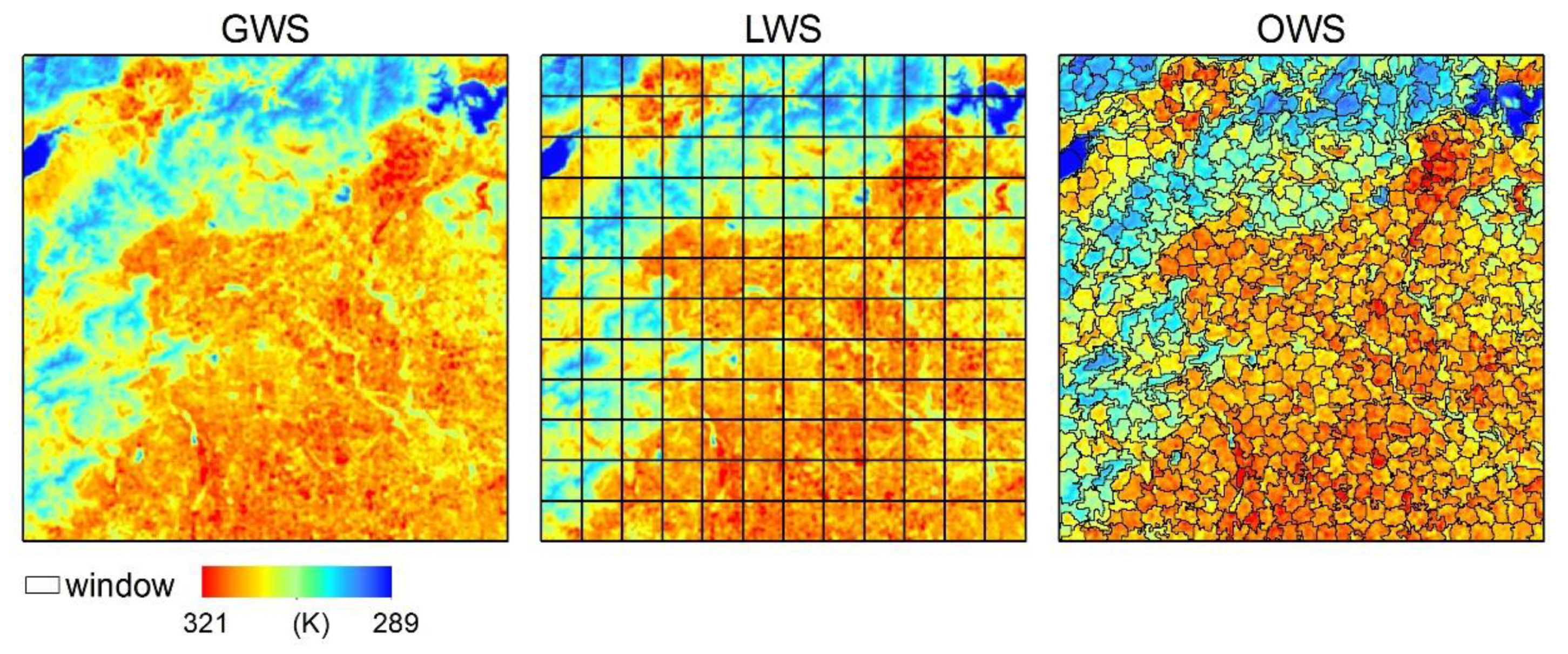
To determine the relationship between the kernels and the LST, a regression window is required. There are two widely used regression windows, namely the global window and the local window. As shown in Figure 1, the GWS indicates that the function relationship is obtained in the whole image and that all pixels correspond to one unique function relationship [14,15]. For the LWS, every moving window has a unique function relationship, and those pixels within the same window have the same function relationship [27]. The moving window in the LWS is square with the same size as that shown in Figure 1.
However, the window size and window shape in the OWS are different from each other (see Figure 1). The window of the OWS is derived via segmentation algorithms, which group pixels similar in color and other properties [34]. Pixels with similar properties in a neighborhood are classified into one object-based window via segmentation algorithms. Both VNIR data and the thermal infrared (TIR) data can be used for segmentation. Since the function relationships of each object-based window are regressed at a low resolution, we use the low-resolution LST as the input to the segmentation. In this paper, we apply the widely used SLIC algorithm, which generates superpixels by applying a k-means clustering approach classifying the input pixels into multiple classes based on their inherent distance from each other [33,36], to obtain the object-based window. The compactness (one important segmentation parameter) of all the segmentation procedures is set to a certain value, and the segmentation scales determine the counts of the objects.
The segmentation scale of the segmentation algorithm determines the size of the object-based windows. For example, when the segmentation scale is set to 100, the whole image is segmented into 100 sub-objects. Accordingly, there are 100 object-based windows, and the window size is determined by the homogeneities of the objects. Moreover, the larger the segmentation scale is, the smaller the size of the object-based window. When the window size is too small, there are not enough training samples for regression, and the function relationship within the window is less efficient in predicting high-resolution LST. When the window size is too large, the heterogeneities among the pixels in the window increase, making the relationship between the kernels and LST more complicated and thus decreasing the accuracy of DLST. Moreover, a larger window that includes more training samples increases the computational complexity [30]. Hence, an optimal segmentation scale that considers the accuracy and computational cost is required for the OWS.
As the ICAD introduced, the optimal moving window size for the LWS varies with the resolution ratio between pre- and post-disaggregated LSTs. Specifically, semivariograms of LST images with different spatial resolutions indicate that coarser images, which are more homogeneous between pixels than fine-resolution images, require more pixels for a stable regression [30]. Hence, we apply a similar selection strategy to determine the optimal segmentation scale for the OWS. Here, we use the number of pixels within the object-based window at high resolution to quantify the window size. The optimal number of pixels in an object-based window can be obtained by the following equation,
where indicates the optimal number of pixels in an object-based window; and are the slope and constant, respectively; and and are the spatial resolutions of the pre- and post-disaggregated LSTs, respectively. Here, we use a linear function to represent the relationship between the optimal number of pixels and the downscaling ratio () due to the simplicity of the linear function and the fact that its validity is supported by the analysis in Section 4.1. The coefficients (i.e., k and b) of Equation (7) are determined by training samples evaluated via root mean square error (RMSE), which provide the optimal number of pixels and downscaling ratio. Once the optimal number of pixels in an object-based window is determined, the optimal segmentation scale is easily obtained from the whole image.
3. Study Area and Data
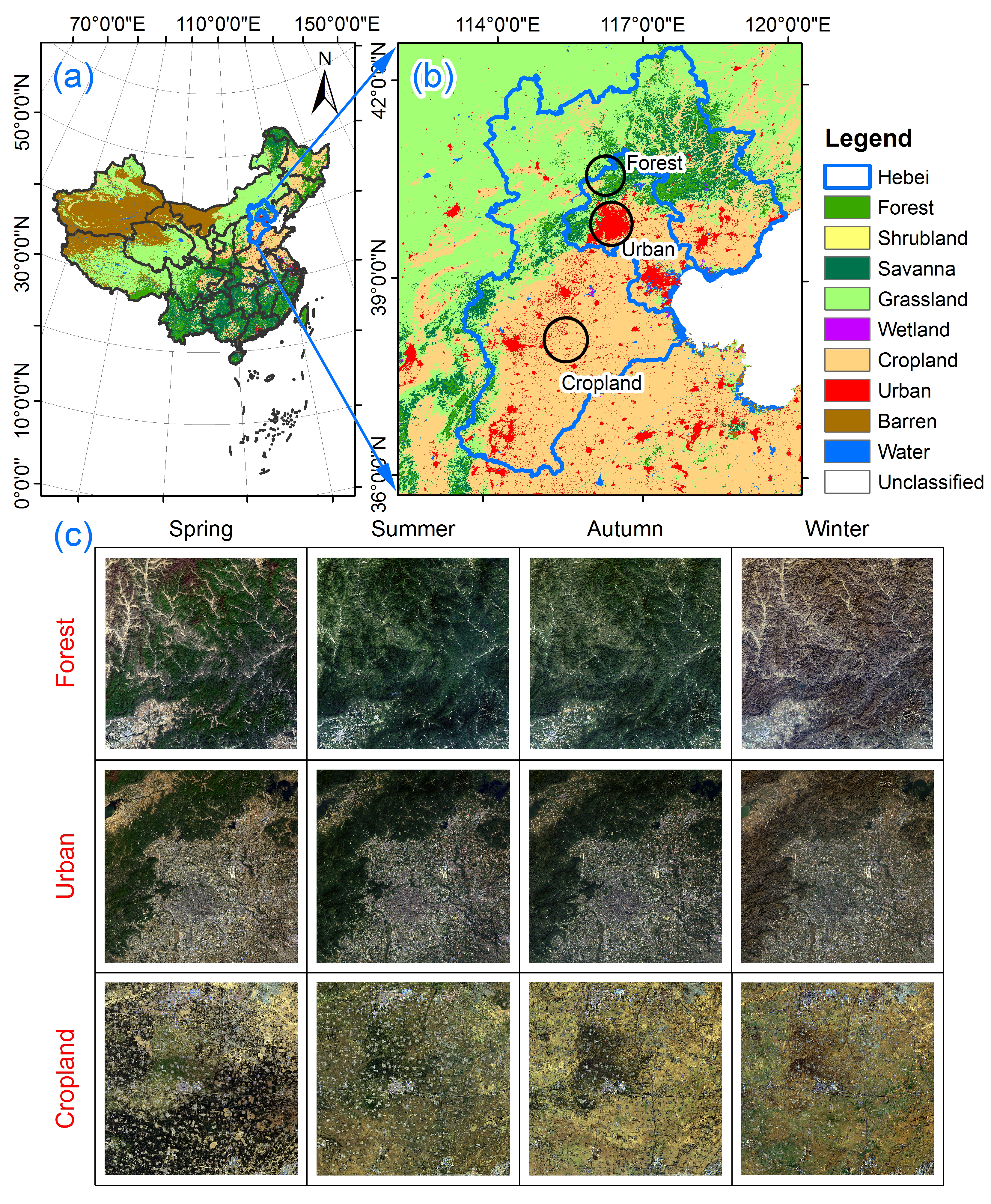
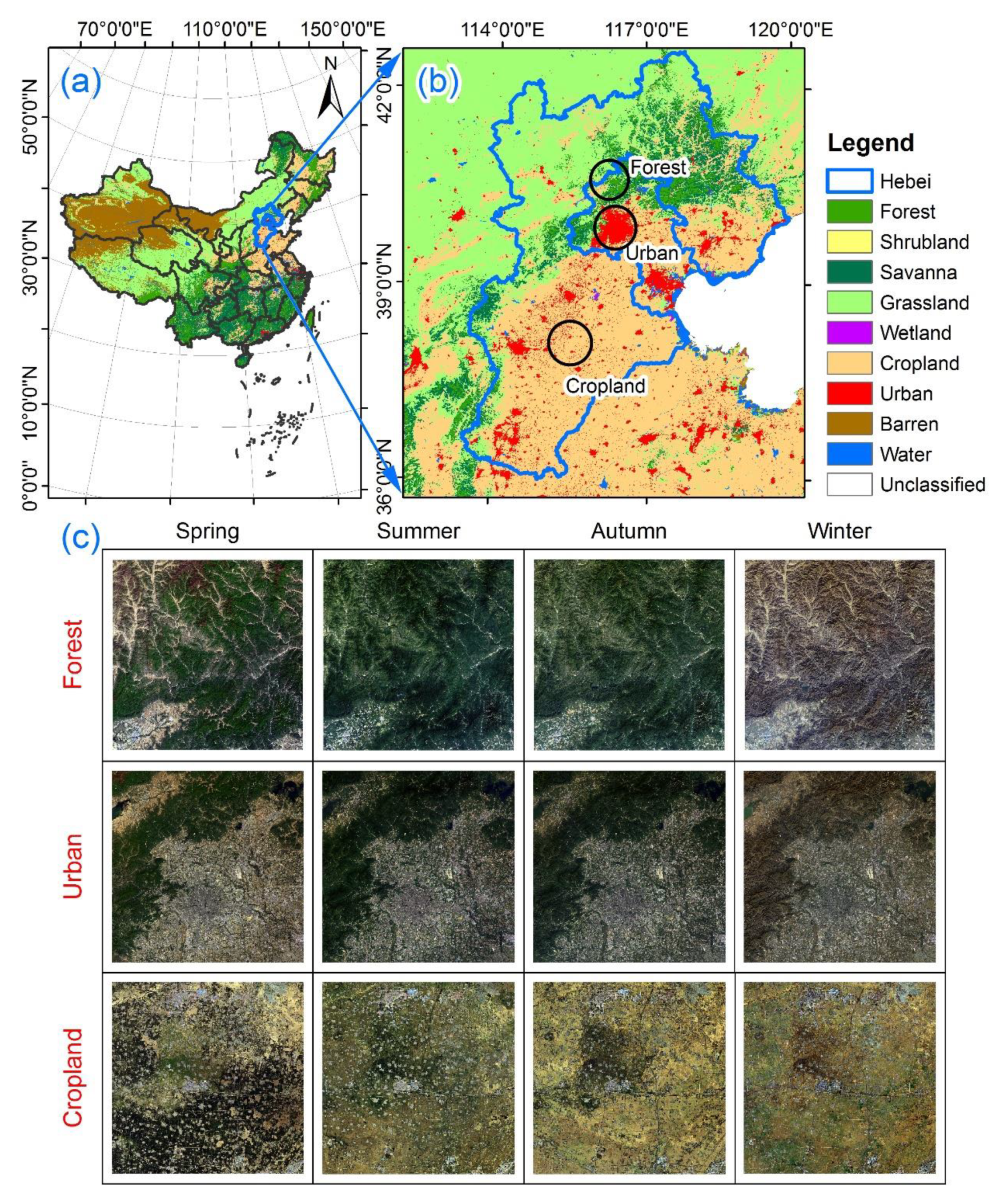
Here, we select three different study areas located in forest, urban and cropland areas. One of the three study areas is in Hebei Province and two are in Beijing (see Figure 2a,b). The forest area is located in the north of Beijing and is mainly covered by forest, with an altitude ranging from 60 m to 2000 m. In addition, this area is not always covered by vegetation, especially in winter, when bare soil takes the place of vegetation. The urban area is located in the central city of Beijing and is mainly covered by impervious surfaces and partly by vegetation. The cropland area is located in Hebei Province and is mainly covered by bare soil, with crops changing from spring to winter. The climate of these three study areas is a sub-humid warm temperature continental climate. In addition, cloud-free images of all study areas collected from spring to winter are used for prediction (see Figure 2c), and the acquisition dates of the images are listed in Table 1.
Landsat 8 datasets (downloaded from https://glovis.usgs.gov/) were used for this research. The VNIR channels (spatial resolution: 30 m) were used as kernels, while the TIR channel (band 10) with a 100 m resolution was used for retrieving LSTs by a single channel algorithm [37]. In addition, with the “aggregation-then-disaggregation” strategy, the original 100 m-resolution LSTs retrieved from the Landsat 8 TIR band were aggregated into 300 m, 600 m, and 900 m resolutions to serve as low-resolution LSTs, so were the kernels.
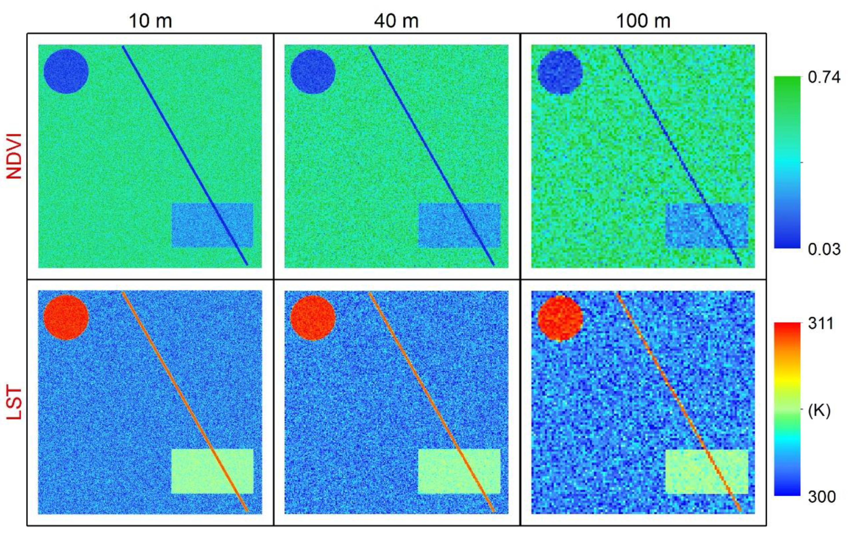
The simulated datasets aimed to explore the strengths and limitations of the OWS compared with the GWS and LWS. This study simulated linear, circular, and rectangular objects by assigning each pixel a digital number of 0–255. These objects represent real-world objects such as buildings, roads, water, bare soils and vegetation [38]. Because the NDVI was used as the kernel in this study, we simulated the NDVI by randomly assigning different ranges of NDVI values to different objects (Figure 3). Then, the LSTs were obtained via known function relationships between the NDVI and the LST (Figure 3). Here, we used four function relationships obtained from the Landsat 8 data, and the coefficients of these functions are shown in Table 2.
4. Results
4.1. Relationship between the Optimal Window Size and the Downscaling Ratio
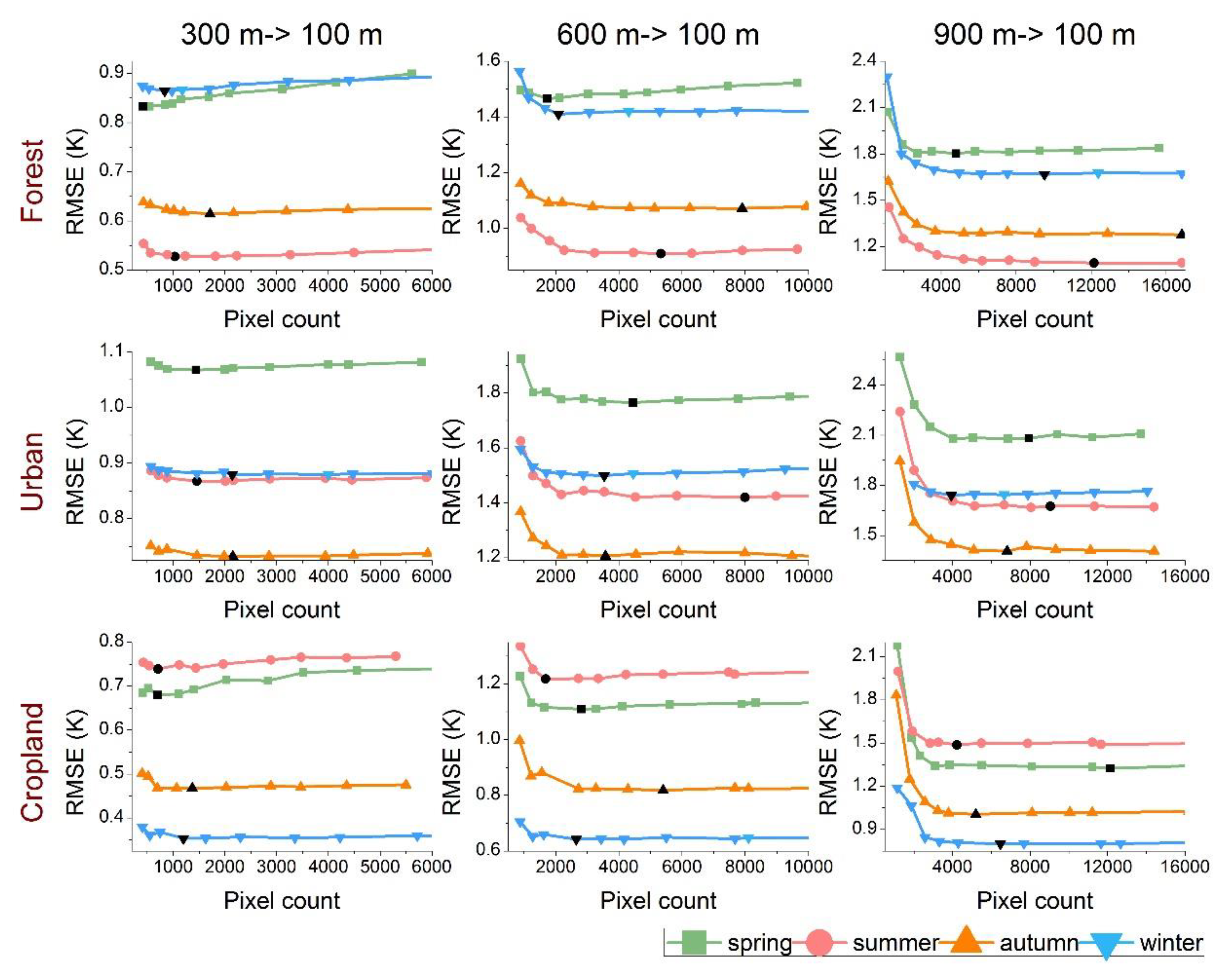
The segmentation scale of the segmentation algorithm determines the size of the object-based windows. Because the optimal segmentation scale for thermal sharpening remains unknown, we downscale the coarse-resolution LSTs via different segmentation scales. As shown in Figure 4, at different downscaling ratios, the accuracies of the downscaled LSTs are mostly lower when the pixel number of a window is extremely small. This result is because the small number of pixels is not able to obtain a stable function relationship between the kernels and the LST. When the number of pixels of a window increases, the accuracy improves accordingly. However, when the number of pixels of a window increases to a certain value, the accuracy does not improve and decreases slightly. This finding is because a larger number of pixels usually corresponds to a larger heterogeneity among the pixels, which makes the unique function relationship between the kernels and the LST less efficient in predicting complicated high-resolution LSTs.
In addition, the difference between the lowest accuracy and the optimal accuracy is different at different downscaling ratios. In detail, the difference is approximately 0.05 K when the downscaling ratio is three, approximately 0.2 K for the downscaling ratio of six and approximately 0.6 K for the downscaling ratio of nine. The more evident improvement at the downscaling ratio of nine indicates the importance for the OWS to determine the optimal segmentation scale when the downscaling ratio is large. Moreover, the optimal number of pixels of the object-based window corresponding to the lowest RMSE value is located in a specific range. For example, the optimal numbers of pixels are mainly less than 2000 in all three different areas when the downscaling ratio is three, the optimal numbers of pixels are between 2000 and 8000 when the downscaling ratio is six, and those at the downscaling ratio of nine are between 4000 and 16,000. These results indicate the positive correlation between the optimal number of pixels and the downscaling ratio. In other words, a coarser image requires a larger number of pixels in the regression window [30].
The results for different seasons and study areas have similar regular patterns, including the overall trend of the accuracies varying with different numbers of pixels and the ranges of the optimal numbers of pixels for different downscaling ratios. Although the curve of the accuracy for the forest area in spring at the downscaling ratio of three is not totally similar to that in other seasons (Figure 4), the optimal number of pixels is smaller than that in other seasons, and the lowest accuracies occur in regions with a larger number of pixels. These results may be due to the lower efficiency of the function relationship between the kernels and the LST in spring since the land cover contains a portion of bare soil. When the window size increases, the pixels within the window become more heterogeneous, which decreases the reliability of the function relationship. However, the overall trend of this curve is still similar to that of the other curves; specifically, the RMSE value of the curve increases when the number of pixels increases above the optimal number of pixels.
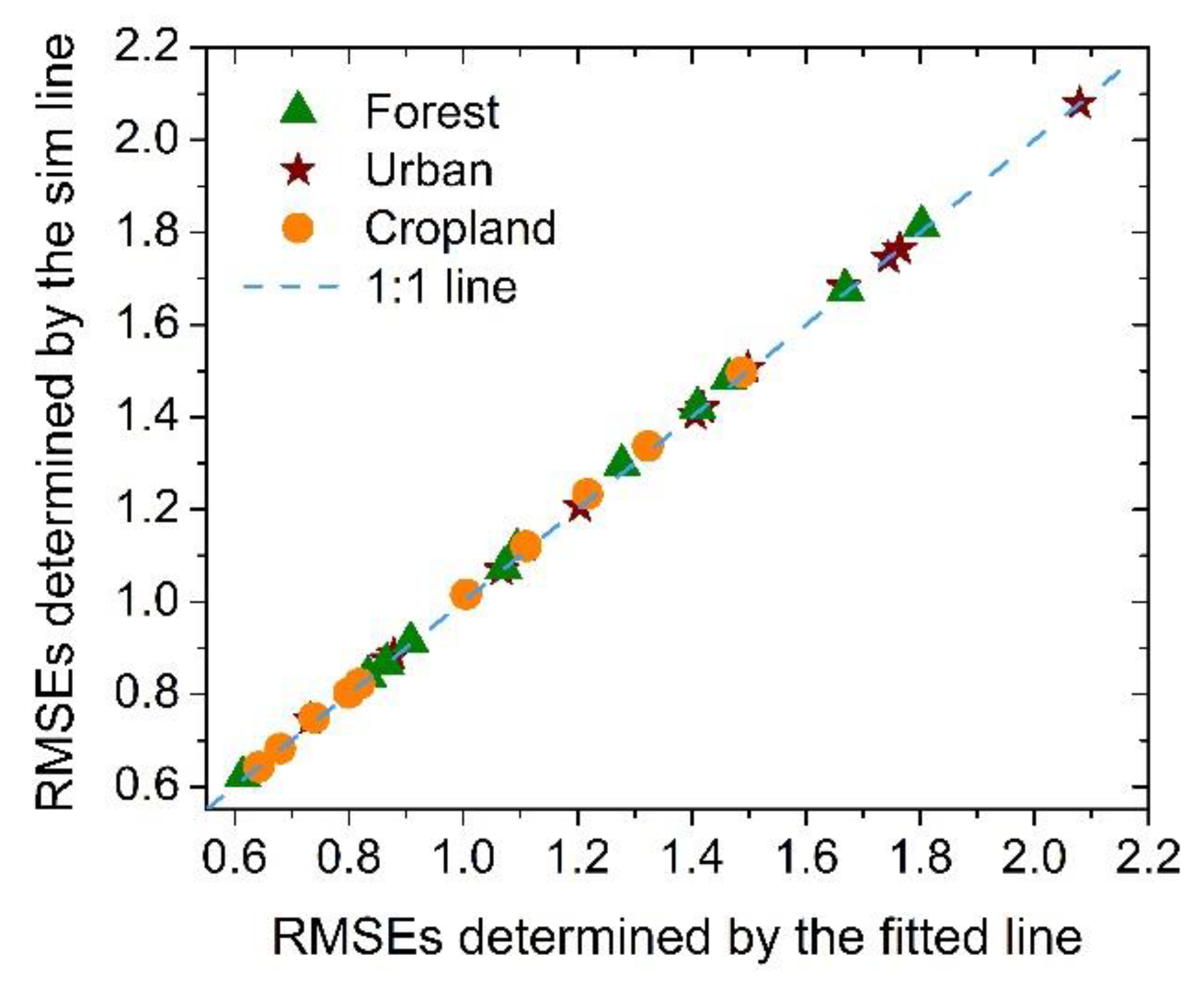
Figure 4 shows that the optimal number of pixels within an object-based window is positively correlated with the downscaling ratio since the optimal number of pixels increases from approximately 1000 to 10,000 with increasing downscaling ratio. We regress the downscaling ratios and the optimal numbers of pixels from the above samples using Equation (7) and obtain the results shown in Figure 5. The coefficients k and b of the fitted line are 1136.63 and −2338.73, respectively. In addition, the R2 value is 0.55 and the P value is less than 0.01 for the regression, and these results prove the reliability of the assumption that the optimal number of pixels and the downscaling ratio have a linear correlation relationship. To simplify the use of the selection strategy for the optimal segmentation scale, we use a simplified fitted line to replace the fitted line (Figure 5). The coefficients k and b for the simplified fitted line are 1000 and −2000 respectively. The accuracies determined by the simplified fitted line only decrease by approximately 0.01 K compared with those determined by the fitted line (Figure 6).
4.2. Comparisons with the LWS and GWS (Test with the Landsat 8 Data)
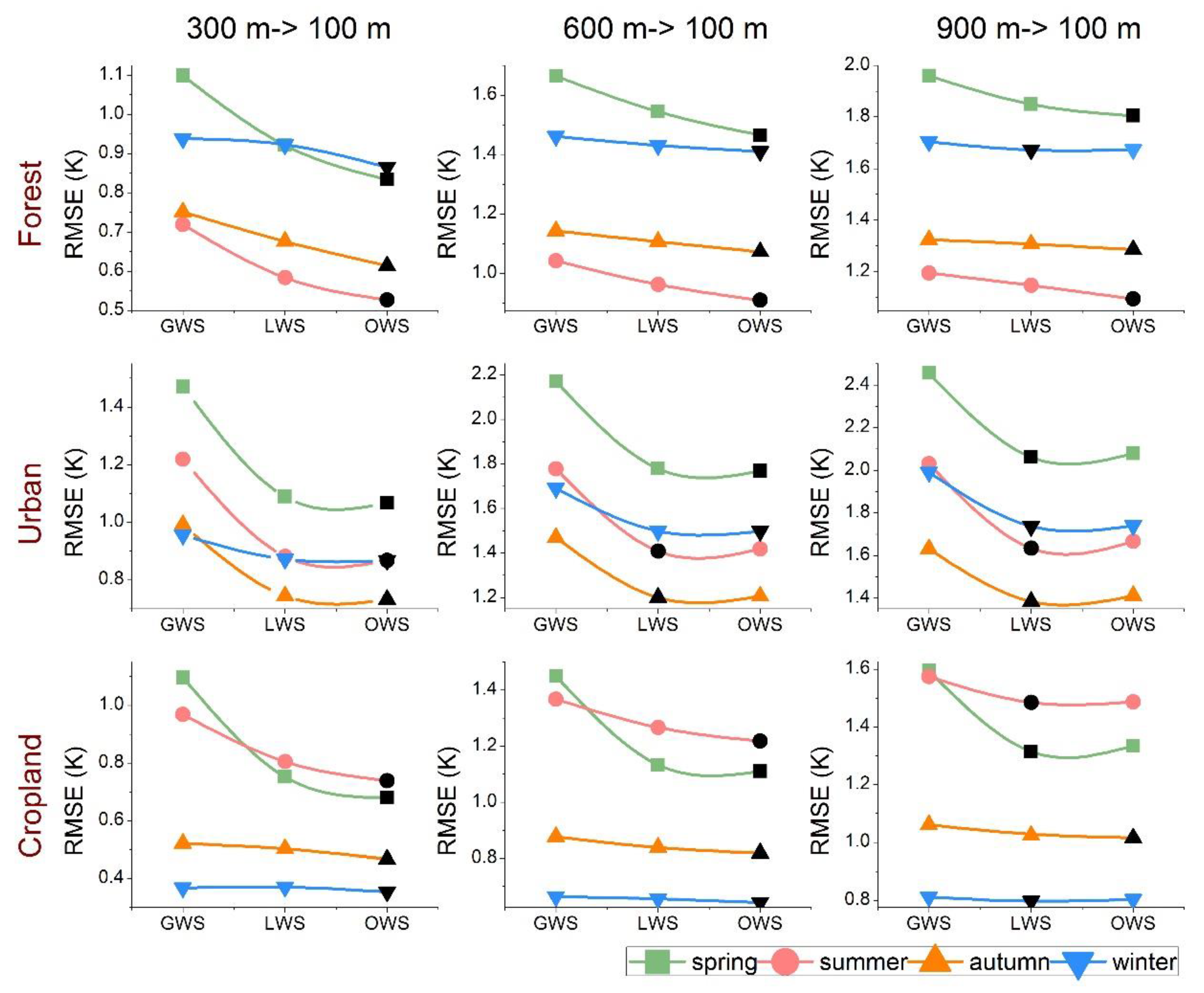
We compare the results of the OWS with those of the GWS and LWS for different land covers in four seasons. As shown in Figure 7, when the downscaling ratio is three, the OWS performs better than both the GWS and LWS for the different land covers in all seasons. Compared with the GWS, the OWS improves the accuracy by approximately 0.21 K when the downscaling ratio is three. Compared with the LWS, the improvement by the OWS is slight (by 0.04 K). When the downscaling ratio is six, the OWS still performs better than both the GWS and LWS in most instances. The improvement by the OWS compared with the GWS is 0.19 K, while that compared with the LWS is 0.02 K. Although the accuracies of the OWS for the urban area are slightly lower than those of the LWS in summer and autumn, the differences are only 0.01 K and 0.006 K for summer and autumn, respectively. When the downscaling ratio is nine, the OWS still performs better than the GWS, with an improvement of 0.16 K. However, compared with the LWS, the OWS only slightly improves by 0.001 K. Moreover, the OWS even performs more poorly than the LWS for the urban area, with a slightly higher RMSE value by 0.02 K in all seasons. This result is because the pixels with a resolution of 900 m contain more land cover types than those with a resolution of 600 m or 300 m over the urban area, and this effect makes the segmented objects less homogeneous between pixels. Hence, the regression relationship within the object-based window is less efficient in predicting high-resolution LSTs.
As shown in Figure 7, the improvements by the OWS compared with the GWS are higher for the urban area than those for the forest and cropland areas; the RMSE value decreases by 0.3 K at different downscaling ratios, while those for the forest and cropland areas only decrease the RMSE value by 0.12 K and 0.14 K, respectively. These results are because the forest and cropland areas are more homogenous than the urban area; in the forest and cropland areas, even with the GWS, the regression relationship between the kernels and LST is efficient in predicting the LSTs of the whole image. However, the urban area is much more complicated, and the correlations between the kernels and LST vary with the land cover type. The unique relationship obtained via the GWS is less efficient over different land cover types. Hence, the OWS provides training samples with more similarities between pixels, and these training samples are used for regression and improving the accuracies of DLST over the urban area.
Using the comparisons with the GWS and LWS for different land covers in all seasons, we find that the improvement by the OWS is larger when the resolution of the pre-disaggregated LST is finer. This finding is because the segmented objects based on finer-resolution LST are more homogeneous both between and within pixels than those based on coarser-resolution LST. Accordingly, the more homogenous the training samples are within the regression window, the more stable the function relationship established between the kernels and LST [13].
Figure 8 shows the DLST for the urban area. The OWS has more similar spatial details than the LWS when the downscaling ratio is three (see Figure 8e,f). However, when we downscale the 600 m and 900 m-resolution LSTs into a 100 m resolution, a grid effect appears in all downscaled LSTs via the GWS, LWS and OWS (see Figure 8g–l). This grid effect is due to the nonlinear statistical regression tool used here since the function relationship is often ill-defined over heterogeneous regions [24]. Regression tools that are based on machine learning techniques, e.g., the RF regression tool, which is flexible over different land cover types, could reduce this shortcoming of the nonlinear statistical regression tool [24].
4.3. Comparisons with the LWS and GWS (Test with the Simulated Data)
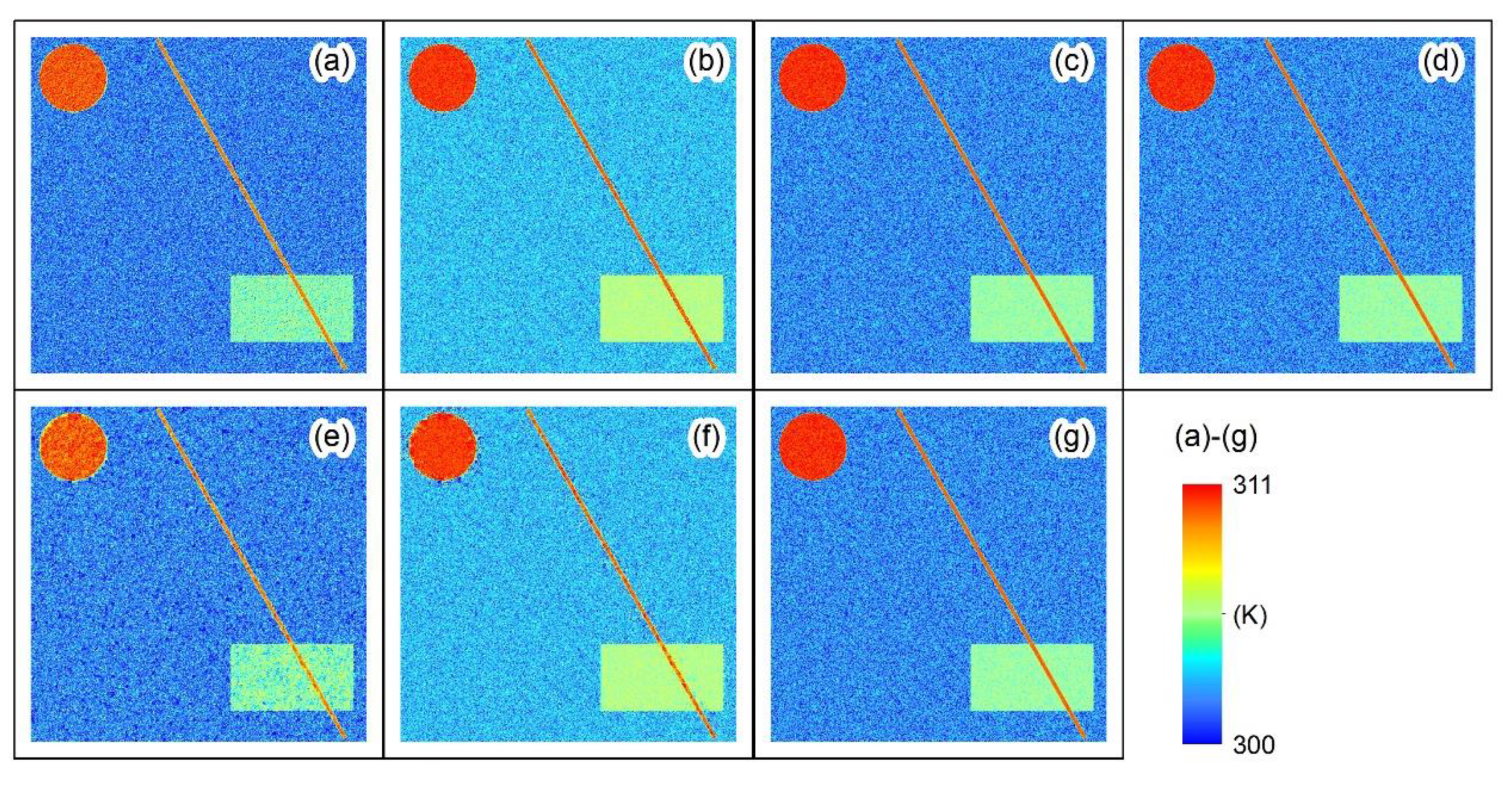
To further explore the performance of the OWS compared with the GWS and LWS, we applied the DLST with the simulated data. As shown in Figure 9, the OWS performs better than both the GWS and LWS at all downscaling ratios. When the downscaling ratio is four, the OWS decreases the RMSE by 0.42 K and 0.16 K compared with the GWS and LWS, respectively. When the downscaling ratio is ten, the OWS improves the accuracy by 0.46 K and 0.22 K compared with that of the GWS and LWS, respectively. These improvements are greater than those tested with the Landsat 8 data (Section 4.2), and these results are because the pixels within the simulated objects are more homogeneous than those in the derived object-based windows via the segmentation algorithm.
In addition, the adaptability of the OWS to different object shapes is stronger than that of the GWS and LWS. As shown in Figure 9e,f, the edges of the circle and line are less clear than those in Figure 9g. Moreover, the edges of objects in the GWS and LWS are blurrier when the downscaling ratio is larger. However, the edges of objects in the OWS are always clear regardless of the size of the downscaling ratio (see Figure 9c,g). These results indicate the superiority of the OWS compared with the GWS and LWS when the pixels within the object-based windows are sufficiently homogeneous. Moreover, the segmentation algorithm generates more homogeneous objects when the spatial resolution of the pre-disaggregated image is higher since the pixels at a higher resolution are more homogeneous.
5. Discussion
5.1. Advantages of the OWS
The proposed OWS uses a segmentation algorithm to derive object-based windows for regression according to the heterogeneities among pixels within the window. Tests with the Landsat 8 data and the simulated data show the outperformance of the OWS compared with the GWS and LWS in most cases, and this outperformance is mainly induced by the following properties.
First, the regression window of the OWS is obtained from the segmentation algorithm, and the pixels within this window have similar spectral properties since the segmentation algorithm tends to classify neighboring pixels with similar properties into one object [34]. With similar pixels, the regressed function relationship in a window is more robust with small residuals [13]. Moreover, the window shapes of the GWS and LWS are square, which may contain various land cover types, increasing the difficulty in establishing a stable function relationship between the kernels and LST [30]. The window shape of the OWS is not limited to specific shapes, such as a square or circle, and only considers the local anisotropic heterogeneity.
Second, compared with the GWS, the OWS has adjustable window size derived by setting different segmentation scales. The fixed window size of the GWS makes the accuracy of DLST depend only on the regression tool and predictors. However, for the OWS, we can select the optimal window size to implement DLST with both high accuracy and efficiency. Compared with the LWS, both the OWS and LWS have adjustable window sizes. However, the window shape of the LWS is square, which is less effective for objects with different shapes. The OWS has a stronger adaptability to different object shapes than the LWS because the windows of the OWS are based on the objects so that the edges of the objects are not blurred (Section 4.3).
However, in some cases, the performance of the OWS remains less satisfying compared with the LWS when the downscaling ratio is larger than six (Section 4.2). This is because the coarse-resolution pixels contain more land cover types and make the segmented objects less homogeneous, resulting in less similarity of the pixels within the object-based window. However, when we implement the DLST with the simulated data (the object-based windows are simulated rather than derived via the segmentation algorithm), the performance of the OWS is always better than that of both the GWS and LWS regardless of the downscaling ratio (Section 4.3). Therefore, we can infer that the OWS will be more effective than both the GWS and LWS when the resolution of pre-disaggregated LSTs is finer since segmentation algorithms can produce more homogeneous object-based windows for regression at a finer resolution.
5.2. Other Issues
(1) Segmentation algorithms: Segmentation algorithms applied in the extraction of object-based windows have crucial effects on the DLST. The more homogeneous the pixels in the windows are, the more stable the function relationship between the kernels and LST and the higher the accuracy of the DLST [13]. Hence, it will be better to evaluate the performance of the segmentation algorithms to determine the best one.
(2) Possible dependence on the regression tool and kernels for DLST: In this study, we used a nonlinear regression tool rather than a linear tool to implement DLST because the study areas are complicated and contain various land cover types, and a linear regression tool might not be efficient in some cases. Moreover, we did not use machine learning tools such as RF, support vector regression and neural networks, which can decrease the grid effects when the downscaling ratios are larger [24]. It is because these machine learning tools are more time consuming than linear and nonlinear regression tools when used for regression.
We used various kernels for the various study areas considering the land cover types within these regions. Specifically, each region corresponds to unique kernels for the whole image; unlike the classification-based method [20], kernels vary with the classification. Because the classification-based method differs in the implementation details, the training samples are spatially discrete and are less efficient in the LWS and OWS [30]. Moreover, the LWS is reported to be better than the GWS for the classification-based method, because the discrete samples of the classification-based method weaken the spatial difference resulting in a flat surface and then make the DLST unacceptable [30].
6. Conclusions
In this paper, we introduce an OWS for thermal sharpening. The implementation of the OWS includes deriving the object-based windows via segmentation algorithms and regressing the relationship within the windows. Moreover, the optimal segmentation scale is determined by an empirical formula obtained from prior samples.
We implement the OWS in a thermal sharpening procedure over three different regions with Landsat 8 data. The object-based windows of the OWS are obtained via the widely used SLIC algorithm. DLST is implemented via the “aggregation-then-disaggregation” strategy. By setting different segmentation scales, we analyze the trends of the DLST accuracies varying with the window size. In addition, the selection strategy for the optimal number of pixels in a window provided in this paper is also suggested to be reasonable. We also compare the OWS with the GWS and LWS with both Landsat 8 data and simulated data. In the test with the Landsat 8 data, the OWS performs better than the GWS and the LWS when the downscaling ratio is small. When the downscaling ratio increases, the OWS still performs better than the GWS but performs slightly worse than the LWS in some cases. Moreover, the OWS is more effective than the GWS for the urban area compared with the other study areas, which indicates the promising abilities of the OWS over heterogenous areas. In the test with the simulated data, the OWS is always superior to both the GWS and LWS regardless of the size of the downscaling ratios, which is because the simulated data eliminates the heterogeneity within the regression window brought by the segmentation algorithm.
The proposed OWS is less limited by the size and shape of the regression window compared with the GWS and the LWS. By applying segmentation algorithms with higher accuracy to derive object-based windows, the OWS has the potential to sharpen LSTs to very high resolutions for urban thermal environment applications. Moreover, the efficient regression tools and optimal kernels will also benefit the performance of the OWS. Future improvements might include the considerations of the geometry effect over urban areas and the dynamic change of LSTs to generate diurnal super-high-resolution LSTs.
Author Contributions
H.X. conceived, designed, and performed the study; analyzed the data; and wrote the paper. Y.C. assisted with the suggestion of the method. J.Q. reviewed this paper and provided suggestions and J.L. helped with editing the paper.
Funding
This work was supported in part by the National Natural Science Foundation of China under Grants 41771448 and 41571342, in part by the Project of State Key Laboratory of Earth Surface Processes and Resource Ecology under Grant 2017-ZY-03, in part by the Science and Technology Plans of Ministry of Housing and Urban-Rural Development of the People’s Republic of China and Opening Projects of Beijing Advanced Innovation Center for Future Urban Design, Beijing University of Civil Engineering and Architecture under Grants UDC2017030212 and UDC201650100, and in part by the Beijing Laboratory of Water Resources Security.
Acknowledgments
We thanked Huang Wei of Beijing Normal University who provided us with the codes of the segmentation algorithms.
Conflicts of Interest
The authors declare no conflict of interest.
References
- Kustas, W.; Anderson, M. Advances in thermal infrared remote sensing for land surface modeling. Agric. For. Meteorol. 2009, 149, 2071–2081. [Google Scholar] [CrossRef]
- Li, F.; Kustas, W.P.; Anderson, M.C.; Prueger, J.H.; Scott, R.L. Effect of remote sensing spatial resolution on interpreting tower-based flux observations. Remote Sens. Environ. 2008, 112, 337–349. [Google Scholar] [CrossRef]
- Kustas, W. Effects of remote sensing pixel resolution on modeled energy flux variability of croplands in iowa. Remote Sens. Environ. 2004, 92, 535–547. [Google Scholar] [CrossRef]
- Cammalleri, C.; Anderson, M.C.; Ciraolo, G.; D’Urso, G.; Kustas, W.P.; La Loggia, G.; Minacapilli, M. Applications of a remote sensing-based two-source energy balance algorithm for mapping surface fluxes without in situ air temperature observations. Remote Sens. Environ. 2012, 124, 502–515. [Google Scholar] [CrossRef]
- Zhou, J.; Chen, Y.; Wang, J.; Zhan, W. Maximum nighttime urban heat island (uhi) intensity simulation by integrating remotely sensed data and meteorological observations. IEEE J. Sel. Top. Appl. Earth Obs. Remote Sens. 2011, 4, 138–146. [Google Scholar] [CrossRef]
- Quan, J.; Chen, Y.; Zhan, W.; Wang, J.; Voogt, J.; Wang, M. Multi-temporal trajectory of the urban heat island centroid in beijing, china based on a gaussian volume model. Remote Sens. Environ. 2014, 149, 33–46. [Google Scholar] [CrossRef]
- Streutker, D.R. Satellite-measured growth of the urban heat island of houston, texas. Remote Sens. Environ. 2003, 85, 282–289. [Google Scholar] [CrossRef]
- Xia, H.; Chen, Y.; Quan, J. A simple method based on the thermal anomaly index to detect industrial heat sources. Int. J. Appl. Earth Obs. Geoinf. 2018, 73, 627–637. [Google Scholar] [CrossRef]
- Blackett, M. An initial comparison of the thermal anomaly detection products of modis and viirs in their observation of indonesian volcanic activity. Remote Sens. Environ. 2015, 171, 75–82. [Google Scholar] [CrossRef]
- Zhan, W.; Chen, Y.; Zhou, J.; Wang, J.; Liu, W.; Voogt, J.; Zhu, X.; Quan, J.; Li, J. Disaggregation of remotely sensed land surface temperature: Literature survey, taxonomy, issues, and caveats. Remote Sens. Environ. 2013, 131, 119–139. [Google Scholar] [CrossRef]
- Xia, H.; Chen, Y.; Li, Y.; Quan, J. Combining kernel-driven and fusion-based methods to generate daily high-spatial-resolution land surface temperatures. Remote Sens. Environ. 2019, 224, 259–274. [Google Scholar] [CrossRef]
- Zhan, W.; Chen, Y.; Zhou, J.; Li, J.; Liu, W. Sharpening thermal imageries: A generalized theoretical framework from an assimilation perspective. IEEE Trans. Geosci. Remote Sens. 2011, 49, 773–789. [Google Scholar] [CrossRef]
- Gao, F.; Kustas, W.; Anderson, M. A data mining approach for sharpening thermal satellite imagery over land. Remote Sens. 2012, 4, 3287–3319. [Google Scholar] [CrossRef]
- Kustas, W.P.; Norman, J.M.; Anderson, M.C.; French, A.N. Estimating subpixel surface temperatures and energy fluxes from the vegetation index–radiometric temperature relationship. Remote Sens. Environ. 2003, 85, 429–440. [Google Scholar] [CrossRef]
- Agam, N.; Kustas, W.P.; Anderson, M.C.; Li, F.; Neale, C.M.U. A vegetation index based technique for spatial sharpening of thermal imagery. Remote Sens. Environ. 2007, 107, 545–558. [Google Scholar] [CrossRef]
- Inamdar, A.K.; French, A. Disaggregation of goes land surface temperatures using surface emissivity. Geophys. Res. Lett. 2009, 36, 436–448. [Google Scholar] [CrossRef]
- Nichol, J. An emissivity modulation method for spatial enhancement of thermal satellite images in urban heat island analysis. Photogramm. Eng. Remote Sens. 2009, 75, 547–556. [Google Scholar] [CrossRef]
- Stathopoulou, M.; Cartalis, C. Downscaling avhrr land surface temperatures for improved surface urban heat island intensity estimation. Remote Sens. Environ. 2009, 113, 2592–2605. [Google Scholar] [CrossRef]
- Zha, Y.; Gao, J.; Ni, S. Use of normalized difference built-up index in automatically mapping urban areas from tm imagery. Int. J. Remote Sens. 2003, 24, 583–594. [Google Scholar] [CrossRef]
- Yang, G.; Pu, R.; Zhao, C.; Huang, W.; Wang, J. Estimation of subpixel land surface temperature using an endmember index based technique: A case examination on aster and modis temperature products over a heterogeneous area. Remote Sens. Environ. 2011, 115, 1202–1219. [Google Scholar] [CrossRef]
- Dominguez, A.; Kleissl, J.; Luvall, J.C.; Rickman, D.L. High-resolution urban thermal sharpener (huts). Remote Sens. Environ. 2011, 115, 1772–1780. [Google Scholar] [CrossRef]
- Huete, A.R. A soil-adjusted vegetation index (savi). Remote Sens. Environ. 1988, 25, 295–309. [Google Scholar] [CrossRef]
- Keramitsoglou, I.; Kiranoudis, C.T.; Qihao, W. Downscaling geostationary land surface temperature imagery for urban analysis. IEEE Geosci. Remote Sens. Lett. 2013, 10, 1253–1257. [Google Scholar] [CrossRef]
- Hutengs, C.; Vohland, M. Downscaling land surface temperatures at regional scales with random forest regression. Remote Sens. Environ. 2016, 178, 127–141. [Google Scholar] [CrossRef]
- Xia, H.; Chen, Y.; Zhao, Y.; Chen, Z. “Regression-then-fusion” or “fusion-then-regression”? A theoretical analysis for generating high spatiotemporal resolution land surface temperatures. Remote Sens. 2018, 10, 1382. [Google Scholar] [CrossRef]
- Yang, Y.; Cao, C.; Pan, X.; Li, X.; Zhu, X. Downscaling land surface temperature in an arid area by using multiple remote sensing indices with random forest regression. Remote Sens. 2017, 9, 789. [Google Scholar] [CrossRef]
- Jeganathan, C.; Hamm, N.A.S.; Mukherjee, S.; Atkinson, P.M.; Raju, P.L.N.; Dadhwal, V.K. Evaluating a thermal image sharpening model over a mixed agricultural landscape in india. Int. J. Appl. Earth Obs. Geoinf. 2011, 13, 178–191. [Google Scholar] [CrossRef]
- Zhukov, B.; Oertel, D.; Lanzl, F.; Reinhackel, G. Unmixing-based multisensor multiresolution image fusion. IEEE Trans. Geosci. Remote Sens. 1999, 37, 1212–1226. [Google Scholar] [CrossRef]
- Chen, X.; Li, W.; Chen, J.; Rao, Y.; Yamaguchi, Y. A combination of tsharp and thin plate spline interpolation for spatial sharpening of thermal imagery. Remote Sens. 2014, 6, 2845–2863. [Google Scholar] [CrossRef]
- Gao, L.; Zhan, W.; Huang, F.; Quan, J.; Lu, X.; Wang, F.; Ju, W.; Zhou, J. Localization or globalization? Determination of the optimal regression window for disaggregation of land surface temperature. IEEE Trans. Geosci. Remote Sens. 2017, 55, 477–490. [Google Scholar] [CrossRef]
- Liu, M.Y.; Tuzel, O.; Ramalingam, S.; Chellappa, R. Entropy rate superpixel segmentation. In Proceedings of the Computer Vision and Pattern Recognition, Colorado Springs, CO, USA, 20–25 June 2011; pp. 2097–2104. [Google Scholar]
- Yao, J.; Boben, M.; Fidler, S.; Urtasun, R. Real-time coarse-to-fine topologically preserving segmentation. In Proceedings of the Computer Vision and Pattern Recognition, Boston, MA, USA, 7–12 June 2015; pp. 2947–2955. [Google Scholar]
- Achanta, R.; Shaji, A.; Smith, K.; Lucchi, A.; Fua, P.; Süsstrunk, S. Slic superpixels compared to state-of-the-art superpixel methods. IEEE Trans. Pattern Anal. Mach. Intell. 2012, 34, 2274–2282. [Google Scholar] [CrossRef] [PubMed]
- Stutz, D.; Hermans, A.; Leibe, B. Superpixels: An evaluation of the state-of-the-art. Comput. Vis. Image Underst. 2018, 166, 1–27. [Google Scholar] [CrossRef] [Green Version]
- Lillo-Saavedra, M.; García-Pedrero, A.; Merino, G.; Gonzalo-Martín, C. Ts2urf: A new method for sharpening thermal infrared satellite imagery. Remote Sens. 2018, 10, 249. [Google Scholar] [CrossRef]
- Lalaoui, L.; Mohamadi, T.; Djaalab, A. New method for image segmentation. Procedia Soc. Behav. Sci. 2015, 195, 1971–1980. [Google Scholar] [CrossRef]
- Jimenez-Munoz, J.C.; Sobrino, J.A.; Skokovic, D.; Mattar, C.; Cristobal, J. Land surface temperature retrieval methods from landsat-8 thermal infrared sensor data. IEEE Geosci. Remote Sens. Lett. 2014, 11, 1840–1843. [Google Scholar] [CrossRef]
- Quan, J.; Zhan, W.; Ma, T.; Du, Y.; Guo, Z.; Qin, B. An integrated model for generating hourly landsat-like land surface temperatures over heterogeneous landscapes. Remote Sens. Environ. 2018, 206, 403–423. [Google Scholar] [CrossRef]
Figure 1.
Window strategies. The background image is a 100 m-resolution LST derived from Landsat 8 data.
Figure 1.
Window strategies. The background image is a 100 m-resolution LST derived from Landsat 8 data.

Figure 2.
Three different study areas and corresponding satellite data. (a) Land cover map of China obtained from the Moderate Resolution Imaging Spectroradiometer (MODIS) yearly land cover product in 2017 (the MODIS image was downloaded from https://ladsweb.modaps.eosdis.nasa.gov/); (b) Land cover map of Hebei Province, where the black circles indicate the locations of the three study areas; (c) Study areas of different land cover types ranging from spring to winter; the images were obtained from the RGB true-color composite of Landsat 8.

Figure 3.
Simulated NDVI and LST data. The 10 m, 40 m and 100 m notations indicate the spatial resolutions of the simulated data. The 40 m and 100 m-resolution data were aggregated from the 10 m-resolution data. The image size of the 10 m-resolution data is 1000 × 1000.
Figure 3.
Simulated NDVI and LST data. The 10 m, 40 m and 100 m notations indicate the spatial resolutions of the simulated data. The 40 m and 100 m-resolution data were aggregated from the 10 m-resolution data. The image size of the 10 m-resolution data is 1000 × 1000.

Figure 4.
RMSEs of the OWS at different segmentation scales. The x-axis is the pixel count in an object-based window and represents the segmentation scales. The black point indicates the minimum RMSE value.
Figure 4.
RMSEs of the OWS at different segmentation scales. The x-axis is the pixel count in an object-based window and represents the segmentation scales. The black point indicates the minimum RMSE value.

Figure 5.
Correlation between the downscaling ratio and the optimal number of pixels in the object-based window.
Figure 5.
Correlation between the downscaling ratio and the optimal number of pixels in the object-based window.

Figure 6.
Scatter plot of the RMSEs determined by the fitted line and the simplified fitted line. “sim line” in the y-axis means the simplified fitted line.
Figure 6.
Scatter plot of the RMSEs determined by the fitted line and the simplified fitted line. “sim line” in the y-axis means the simplified fitted line.

Figure 7.
RMSEs of the results of the GWS and LWS with the optimal accuracy and those of the OWS with the optimal accuracy. The black point indicates the minimum RMSE value among the GWS, LWS and OWS.
Figure 7.
RMSEs of the results of the GWS and LWS with the optimal accuracy and those of the OWS with the optimal accuracy. The black point indicates the minimum RMSE value among the GWS, LWS and OWS.

Figure 8.
Results of DLST for the urban area on May 7, 2017. (a) RGB true-color composite of Landsat 8; (b) subsets of (a); (c) reference LST; (d) GWS (300 m→100 m); (e) LWS (300 m→100 m); (f) OWS: (300 m→100 m); (g) GWS (600 m→100 m); (h) LWS (600 m→100 m); (i) OWS (600 m→100 m); (j) GWS (900 m→100 m); (k) LWS (900 m→100 m); (l) OWS (900 m→100 m).

Figure 9.
Results of DLST based on the simulated data. (a) GWS (40 m→10 m); (b) LWS (40 m→10 m); (c) OWS (40 m→10 m); (d) simulated LST; (e) GWS (100 m→10 m); (f) LWS (100 m→10 m); (g) OWS (100 m→10 m).
Figure 9.
Results of DLST based on the simulated data. (a) GWS (40 m→10 m); (b) LWS (40 m→10 m); (c) OWS (40 m→10 m); (d) simulated LST; (e) GWS (100 m→10 m); (f) LWS (100 m→10 m); (g) OWS (100 m→10 m).


Table 1.
Description of the Landsat 8 data.
| Study Area | Acquisition Date (YY-MM-DD) | Path/Row | Altitude (m) |
|---|---|---|---|
| Forest | 2017-05-07, 2017-07-10, 2017-09-12, 2017-10-30 | 123/32 | 60–2000 |
| Urban | 2017-05-07, 2017-07-10, 2017-09-12, 2017-10-30 | 123/32 | 20–2000 |
| Cropland | 2016-04-18, 2017-07-10, 2017-10-30, 2017-12-17 | 123/34 | 10–50 |
Table 2.
Coefficients of the function relationship used in the simulated data.
| Object | a0 | a1 | a2 |
|---|---|---|---|
| Circle | 38.5 | −10.0 | −6.0 |
| Line | 37.4 | −9.7 | −6.1 |
| Rectangle | 34.4 | −5.7 | −5.1 |
| Background | 33.4 | −4.5 | −5.6 |
1 The function relationship is provided in Equation (3), and the kernels are the NDVI and NDVI2.
© 2019 by the authors. Licensee MDPI, Basel, Switzerland. This article is an open access article distributed under the terms and conditions of the Creative Commons Attribution (CC BY) license (http://creativecommons.org/licenses/by/4.0/).
Share and Cite
MDPI and ACS Style
Xia, H.; Chen, Y.; Quan, J.; Li, J. Object-Based Window Strategy in Thermal Sharpening. Remote Sens. 2019, 11, 634. https://doi.org/10.3390/rs11060634
AMA Style
Xia H, Chen Y, Quan J, Li J. Object-Based Window Strategy in Thermal Sharpening. Remote Sensing. 2019; 11(6):634. https://doi.org/10.3390/rs11060634
Chicago/Turabian StyleXia, Haiping, Yunhao Chen, Jinling Quan, and Jing Li. 2019. "Object-Based Window Strategy in Thermal Sharpening" Remote Sensing 11, no. 6: 634. https://doi.org/10.3390/rs11060634
Note that from the first issue of 2016, this journal uses article numbers instead of page numbers. See further details here.