Full and Simulated Compact Polarimetry SAR Responses to Canadian Wetlands: Separability Analysis and Classification

Abstract

Detailed information on spatial distribution of wetland classes is crucial for monitoring this important productive ecosystem using advanced remote sensing tools and data. Although the potential of full- and dual-polarimetric (FP and DP) Synthetic Aperture Radar (SAR) data for wetland classification has been well examined, the capability of compact polarimetric (CP) SAR data has not yet been thoroughly investigated. This is of great significance, since the upcoming RADARSAT Constellation Mission (RCM), which will soon be the main source of SAR observations in Canada, will have CP mode as one of its main SAR configurations. This also highlights the necessity to fully exploit such important Earth Observation (EO) data by examining the similarities and dissimilarities between FP and CP SAR data for wetland mapping. Accordingly, this study examines and compares the discrimination capability of extracted features from FP and simulated CP SAR data between pairs of wetland classes. In particular, 13 FP and 22 simulated CP SAR features are extracted from RADARSAT-2 data to determine their discrimination capabilities both qualitatively and quantitatively in three wetland sites, located in Newfoundland and Labrador, Canada. Seven of 13 FP and 15 of 22 CP SAR features are found to be the most discriminant, as they indicate an excellent separability for at least one pair of wetland classes. The overall accuracies of 87.89%, 80.67%, and 84.07% are achieved using the CP SAR data for the three wetland sites (Avalon, Deer Lake, and Gros Morne, respectively) in this study. Although these accuracies are lower than those of FP SAR data, they confirm the potential of CP SAR data for wetland mapping as accuracies exceed 80% in all three sites. The CP SAR data collected by RCM will significantly contribute to the efforts ongoing of conservation strategies for wetlands and monitoring changes, especially on large scales, as they have both wider swath coverage and improved temporal resolution compared to those of RADARSAT-2.

1. Introduction

Wetlands are regions where water is the main factor affecting the ecosystem and the associated flora and fauna [1]. In such an environment, the water table is either at or near to the land surface or the land surface is covered by shallow-water [2]. Wetlands are natural infrastructures that facilitate the interactions of soils, water, plants, and animals, thus making them one of the most productive ecosystems. Wetlands serve a number of purposes, including water storage and purification, flood mitigation, storm protection, erosion control, shoreline stabilization, carbon dioxide sequestration, and climate regulation [3]. To support global preservation of wetlands, the Ramsar Convention on Wetlands has been in place since 1971, wherein the main purpose is “the conservation and wise use of wetlands globally” [1]. Over the years, several countries (163 nations as of January 2013), including Canada, have joined to the convention and demonstrated their commitments to wetland preservation.

Over the past two decades, remote sensing tools and data have significantly contributed to wetland mapping and monitoring [4]. Optical remote sensing satellites have long been the main source of Earth Observation (EO) data for vegetation and wetland mapping [5,6], yet cloud cover hinders the acquisition of such data. Consequently, as they are not impacted by solar radiation or weather conditions and can penetrate vegetation canopies (depending on wavelength), Synthetic Aperture Radar (SAR) sensors are of special interest, particularly in geographic regions with chronic cloud cover, such as Canada [7]. The interaction of SAR signal with vegetation canopies depends on SAR wavelengths [8]. Overall, longer wavelengths (e.g., L-band) are preferred for monitoring woody wetlands [8], whereas shorter wavelengths (e.g., C- and X-band) are useful for mapping herbaceous wetlands [9]. Several studies reported of great benefit of L-band data collected by JERS-1 and ALOS PALSAR-1 for inundation and vegetation dynamic mapping in various geographic locations, such as the Amazon floodplain [10,11], the Alligator Rivers region of northern Australia [12], and wetlands in Africa [13]. Other studies demonstrated the capability of shorter wavelengths, such as C-band data collected by ERS-1/2 [14], RADARSAT-1 [15], RADARSAT-2 [16,17], and Sentinel-1 [18] for wetland classification. X-band data collected by TerraSAR-X were also found to be useful for mapping heterogeneous structure of wetland ecosystems and their dynamics, given its high temporal and spatial resolution [19,20].

Wetland phenology also affects SAR backscattering responses of flooded vegetation and depends on complex relation of vegetation height/density and the water level height in the wetland ecosystem [21]. For example, during high water seasons, the classes of swamp forest and freshwater marsh experience different conditions. In particular, an increase in water level height increases the chance of double-bounce scattering for swamps, resulting in an enhanced SAR backscattering response [22]. In contrast, an increase in water level height may decrease the chance of double-bounce scattering for marshes, as it converts double-bounce scattering to the specular scattering mechanism [23]. This results in little backscattering responses on SAR imagery in this case. Vegetative density is another influential factor and was examined in several research. For example, Lu and Known (2008) found that high vegetative density and canopy in swamp forest during the leaf-on season converted double-bounce scattering to volume scattering in southeastern coastal Louisiana wetlands using ERS and RADARSAT-1 imagery, which decreased SAR backscattering responses over swamp forest [24]. Later studies, such as [25,26], found relatively similar results using ALOS PALSAR L-band data for forested wetlands in the Congo River in Africa.

In addition to SAR wavelength and wetland phenology, polarization of SAR signal is also an important factor. Given the capability of full-polarimetric (FP) SAR sensors to collect full scattering information of ground targets, the potential of these sensors for mapping various wetland classes has been well established [27]. In particular, a FP SAR sensor transmits a fully-polarized signal toward ground targets while receiving both fully-polarized and depolarized backscattering responses from a ground target [28]. This configuration also maintains the relative phase between polarization channels, thus allowing the application of advanced polarimetric decomposition methods [29]. The polarimetric decompositions are beneficial for distinguishing similar wetland classes through characterizing various scattering mechanisms of ground targets.

Notably, decomposition techniques allow the polarimetric covariance or coherency matrixes to be separated into three main scattering mechanisms: single/odd-bounce scattering, which represents direct scattering from the vegetation or ground surface (e.g., rough water); double/even-bounce scattering, which represents scattering between, for example, flooded vegetation within smooth open water; and volume scattering, which represents multiple scattering within developed vegetation canopies. As such, several studies reported the success of wetland classification using FP SAR data in different geographic regions, such as China [30], Europe [31], the United States [32], and Canada [33]. However, the main limitations associated with the FP SAR configuration are the time constraints caused by the alternative transmitting of H and V polarizations toward ground targets, the large satellite mass caused by higher system power requirements, and the small swath coverage caused by doubling pulse repetition frequency (PRF) [34]. The small swath coverage precludes the potential of such data for applications on large-scales [35], for example, for the production of daily ice charts and annual crop inventories.

Dual-polarimetric (DP) SAR data cover a larger swath width and, currently, are the main source of SAR observations for operational applications. Such a SAR data configuration is currently available on Sentinel-1 SAR mission satellite of the Copernicus program by the European Space Agency (ESA) [36]. The main purpose of this mission is to provide full, free, and open access SAR observations for environmental monitoring [37]. Furthermore, the 12-days satellite revisit time makes Sentinel-1 SAR data ideal for monitoring phenomena with highly dynamic natures such as wetlands [18,38], as well as assistant with operational applications such as sea ice monitoring [39] and crop mapping [40]. However, insufficient polarimetric information is available within such data. Furthermore, DP SAR data cannot maintain a relative phase between polarization channels, thus diminishing their capability to distinguish similar land and wetland classes through advanced polarimetric decomposition techniques [29]. To move forward with both polarization diversity and swath coverage, the compact polarimetry (CP) SAR configuration was introduced. CP SAR sensors are in the same group as that of DP but differ in terms of the choice of polarization channels [41]. This configuration collects greater polarimetric information compared to that of DP, while covering a much larger swath width relative to that of FP SAR data. CP SAR sensors also maintain the relative phase between two received polarization channels, which further makes them advantageous relative to DP SAR sensors for a variety of applications.

Importantly, the upcoming RADARSAT Constellation Mission (RCM), which is the successor mission to RADARSAT-2, that is planned to be launched in 2019, will have a circularly transmitting, linearly receiving (CTLR) CP mode as one of its main SAR data collection configurations [42]. The main purposes of RCM are to ensure data continuity for RADARSAT-2 users and ameliorate the operational capability of SAR data by leveraging a more advanced spaceborne mission [35]. In particular, RCM comprises three identical small (relative to RADARSAT-2) C-band satellites to gain greater satellite coverage over a much shorter satellite revisit time (only four-day) [43]. This is of great importance for applications, such as maritime surveillance and ecosystem monitoring, which heavily rely on frequent SAR observations.

Various SAR configurations and polarizations are available with RCM. These include single-polarimetry (SP), conventional DP, and CTLR CP modes. In the CTLR mode, RCM transmits a right-circular polarized signal and receives two coherent orthogonal linear (both horizontal and vertical) polarized signals (RH and RV) and their relative phase [44]. 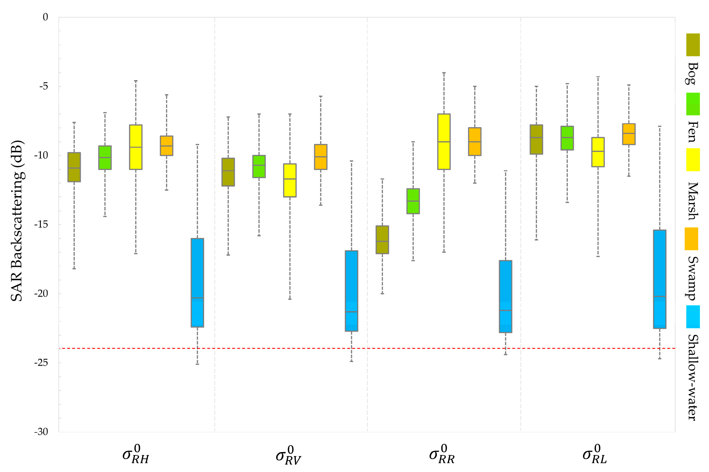Lower PRF and system power and less on-board mass and data volume are other advantages of RCM compared to RADARSAT-2 [45]. Despite these benefits, less polarimetric information is available within CP SAR data compared to that of FP SAR data. Furthermore, Noise Equivalent Sigma Zero (NESZ) values potentially range between −25 to −17 dB for RCM data [43], which are higher than those of RADARSAT-2 in most cases. This decreases the sensitivity of the RCM SAR signal to ground features with low backscattering values, such as open water and sea ice.

It is beneficial to compare both the similarities and differences of CP SAR data collected by RCM with those of RADARSAT-2 in different applications, prior to the availability of RCM data for operational monitoring. Given that maritime surveillance is one the main application of RCM data [45], the potential of simulated or real CP SAR data has been well examined for sea ice classification and monitoring in several recent studies (e.g., [35,41,46,47]). However, the potential of CP SAR data for other applications, such as wetland characterization, remains an active research area, requiring much investigation to fully exploit the capability of such data for other purposes, such as ecosystem monitoring (e.g., agriculture, wetland, and forestry). Notably, two previous studies have highlighted the capability of simulated CP SAR data from RADARSAT-2 for wetland mapping. Brisco et al. (2013) first reported the potential of CP SAR data for wetland classification in southwestern Manitoba, Canada, using 12 CP SAR features but for wetland classes different from typical Canadian wetland classes (i.e., bog, fen, marsh, swamp, and shallow-water, as classified based on the Canadian Wetland Classification System, CWCS) [48]. White et al. (2017) evaluated the potential of simulated CP SAR data from RADARSAT-2 with a larger number of CP features, yet only for peatland classes (i.e., poor fen, open shrub bog, and treed bog) in a small area in Southern Ontario, Canada [49]. However, the latter study exploited the synergy of CP and FP SAR data with digital elevation model (DEM) and Landsat-8 optical data for classifying peatland classes [49]. Although their methodology and results were sound, much investigation is still required to fully understand the compact polarimetric responses of various CP SAR features to standard wetland classes (according to the definition of CWCS).

The present research was built on the knowledge gained from our previous work, wherein the potential of CP SAR features for wetland mapping was investigated [29]. However, unlike in [29], in the present study, three wetland sites were selected and the main objectives here were to identify the most useful CP features for similar wetland class discrimination and to improve image interpretation using both qualitative and quantitative approaches. Specifically, this study aimed to: (1) explore the effect of the difference in polarization between FP (RADARSAT-2) and simulated CP SAR data for the classification of wetland complexes; (2) determine the separability between pairs of wetland classes with various CP SAR features both visually, using box-and-whisker plots, and quantitatively, using the Kolmogorov-Smirnov (K-S) distance measurement; and (3) classify wetland complexes using the most effective CP SAR features using an object-based random forest (RF) algorithm.

2. Study Area and Data

2.1. Study Area and In-Situ Data

The three study areas located in Newfoundland and Labrador, Canada, at the eastern, center, and western portions of the island were selected for this research (see Figure 1). In general, the island of Newfoundland has a humid continental climate, which is greatly affected by the Atlantic Ocean.

The first pilot site is the Avalon area, located in the most eastern part of the island in the Maritime Barren ecoregion. It has an oceanic climate of foggy, cool summers, and relatively mild winters. The second pilot site is the Deer Lake area, located in the the northern (center) portion of the island in the Central Newfoundland ecoregion and experiences a continental climate of cool summers and cold winters. Finally, the third pilot site is the Gros Morne area, located on the extreme western coast of the island, in the Northern Peninsula ecoregion. This area has a maritime-type climate with cool summers and mild winters [50]. As elsewhere in Newfoundland, frequent rain and fog are dominant due to the proximity of the pilot sites to the Atlantic Ocean. This highlights the great significance of SAR data for remote sensing studies for the island.

The study areas contain all wetland classes categorized by the CWCS, namely bog, fen, marsh, swamp, and shallow water, although bog and fen are the most dominant classes. Other land cover classes include urban, upland, and deep water. Figure 2 illustrates examples of land cover classes in the Avalon study area.

For this study, in-situ data were collected over multiple visits during the summers and falls of 2015, 2016, and 2017. Potential and accessible wetland sites in all study areas were flagged based on prior knowledge of wetland sites, interpretation of high resolution Google Earth imagery, and the CWCS definition of wetlands. Other considerations for site visitation included accessibility via public roads and the public and private ownership of lands. Significant effort was devoted to collect in-situ data covering a wide range of wetland and non-wetland classes with vast spatial distributions across all study areas. In each location, one or more Global Positioning System (GPS) points were collected, depending on the size of each wetland class. Digital photographs and ancillary notes (e.g., dominant vegetation, hydrology, dates, and the name of locations) were also recorded to facilitate preparation of the training samples. Notably, data from wetlands of various sizes were collected during the first year of data collection, resulting in the production of several small-size classified polygons. However, wetlands with sizes greater than one ha (where possible) were selected during the following years to restrict the production of small-size polygons to a feasible extent.

Recorded GPS points were then imported in ArcMap10.6, and polygons indicating classified delineated wetlands were produced using a visual interpretation of 50 cm resolution orthophotographs and 5 m resolution RapidEye optical images by remote sensing and biologist experts familiar with the studies areas. Notably, any human error in both recording GPS points during in-situ data collection and preparing the reference polygons may affect the results of separability analysis and classification. Next, polygons were sorted based on their size and alternately assigned to either training or testing groups. This alternative assignment ensured that both the training (~50%) and testing (~50%) polygons had relatively equal numbers of small and large polygons. Furthermore, the training and testing polygons were obtained from independent samples to ensure robust accuracy assessment.

Table 1. Number of training and testing polygons for each class in the three pilot sites.

	Avalon		Deer Lake		Gros Morne
Class	Training	Testing	Training	Testing	Training	Testing
Bog	42	41	16	15	19	19
Fen	20	19	27	27	15	16
Marsh	25	25	12	12	16	15
Swamp	22	23	20	20	21	21
Shallow water	20	20	11	12	13	14
Urban	36	35	17	18	19	19
Deep water	7	8	3	3	3	2
Upland	29	29	12	11	42	43
Total	201	200	118	118	148	149

presents the number of training and testing polygons for each class in the three pilot sites.

2.2. Satellite Imagery

A total number of seven Single Look Complex (SLC) RADARSAT-2 images were used in this study. These images were acquired using the Fine Quad-polarization (FQ) mode on August 2015 from descending orbits (see

Table 2. Characteristics of RADARSAT-2 imagery used in this study.

Pilot Site	Date	# Images	Mode	Image Coverage (km) *	Incidence Angle (°)	NESZ (dB)	Resolution (m) *
Avalon	20150821	2	FQ4	25 × 25	22.1–24.1	−34.6 to −37.8	5.2 × 7.6
Deer Lake	20150810	2	FQ3	25 × 25	20.9–22.9	−34.4 to −37.7	5.2 × 7.6
Gros Morne	20150803	3	FQ2	25 × 25	19.7–21.7	−34 to −38.4	5.2 × 7.6

* Note that image coverage is represented in (ground range × azimuth) and resolution is represented in (slant range × azimuth).

).

Notably, the leaf-on season in Newfoundland starts by late May/early June. August corresponds to the peak of the growing season in the study area, wherein both the vegetative density and water level height are at their optimum. Accordingly, imagery was selected from August, as our recent study demonstrated that flooding status of vegetation is at the highest, resulting in the maximum occurrence of double-bounce scattering at this time period [51].

As indicated in Table 2, RADARSAT-2 images were collected in 2015; our in-situ data used for both classification and separability analysis were collected during the summers and falls of 2015, 2016, and 2017. We assumed that no change had occurred in the wetland properties during the three year interval given very limited human activities in the studies areas. Furthermore, this time difference (i.e., <three years) between satellite data acquisition and the collection of ecological training data is acceptable and agrees with those used in previous research (e.g., [51,52]).

3. Methods

3.1. Full Polarimetric SAR Data Processing

The main preprocessing steps were speckle reduction, orthorectification, and image mosaicking. Speckle reduction is a necessary preprocessing step, as the radiometric quality of SAR images is hindered by speckle noise, which affects subsequent image processing steps (e.g., segmentation and classification) [53]. Accordingly, a 5 × 5 Boxcar filter was employed to suppress speckle and increase the number of looks prior to extraction of polarimetric features. A small filter size was selected, as it maintains the boundaries between natural and human-made objects and is appropriate for wetland classes with small sizes (e.g., swamp and marsh in this study). Orthorectification of de-speckled RADARSAT-2 images was performed in PCI Geomatica’s OrthoEngine 2017 software using the rational function model [54,55]. Satellite orbital information and an external digital elevation model (DEM), released by Natural Resource Canada, were employed for orthorectification. All images were projected into UTM coordinates, zone 22/row T for the Avalon study area and zone 21/ row U for the Deer Lake and Gros Morne study areas, respectively. Two scenes from the Avalon and Deer Lake pilot sites and three from the Gros Morne study region were then mosaicked into single strips of data.

A total of 13 features were extracted from the full polarimetric RADARSAT-2 images. In particular, three SAR backscattering coefficient images, namely ${\sigma }_{HH}^0$, ${\sigma }_{VV}^0$, and ${\sigma }_{HV}^0$, were extracted. ${\sigma }_{HH}^0$ is sensitive to double-bounce scattering and, as such, is useful for discriminating flooded and non-flooded wetland classes [9]. It is also beneficial for discriminating water from non-water (e.g., upland) classes, given its lower sensitivity to surface roughness on water compared to ${\sigma }_{VV}^0$ [9]. ${\sigma }_{VV}^0$ is suitable for distinguishing herbaceous wetland classes, especially bog and fen classes [56]. It is also sensitive to soil moisture [57,58] and is useful for discriminating sparsely vegetated areas. ${\sigma }_{HV}^0$ is sensitive to the vegetation structure and has shown promising results for distinguishing wetland classes [8].

Three incoherent decomposition methods, namely Cloude-Pottier [59], Freeman-Durden [60], and Yamaguchi [61], were also employed. These methods decompose the SAR backscattering responses of distributed ground targets into various scattering mechanisms, which are of great use for discriminating similar wetland classes. This is because wetland classes are characterized by varying scattering mechanisms depending on SAR wavelength, roughness, and vegetation structure through the growing season.

The Cloude-Pottier method is a decomposition that considers three secondary components, including the entropy, anisotropy, and alpha angle, which are derived from eigenvalues and eigenvectors. Entropy ranges from 0 to 1 and indicates the degree of randomness. Lower entropy values demonstrate that a single scattering mechanism is dominant (low depolarization); whereas values approaching 1 suggest that multiple scatterings are present. Anisotropy is the complementary component to entropy and represents the relative importance of the secondary scattering mechanism. The alpha angle varies between 0$°$ and 90$°$ and is also useful for characterizing different scattering mechanisms. Surface, volume, and double-bounce scattering produce low, intermediate, and high alpha angles, respectively.

The Freeman-Durden and Yamaguchi decompositions are known as physical model-based decomposition approaches with three and four components, respectively. In particular, the Freeman-Durden approach, which assumes reflection symmetry, decomposes target scattering as the linear sum of the surface, double-bounce, and volume scattering mechanisms [60]. The Yamaguchi decomposition has similar components as those of Freeman-Durden; however, it benefits from an additional term, known as the helix scattering component. This component takes into account cases of non-reflection symmetry (i.e., the correlation between co- and cross-polarized channels), which usually occur in complex urban areas. Additionally, the volume scattering term of the Yamaguchi decomposition for vegetation was further modified by employing a different probability density function than that used by the Freeman-Durden approach [61].

3.2. Compact Polarimetry SAR Data Processing

The Canada Centre for Mapping and Earth Observation (CCMEO) simulator was used to simulate the RCM CP data [45]. The CCMEO calibrates the RADARSAT-2 SLC product using the Sigma Naught (${\sigma }^0$) calibration. The calibrated product is stored in a 3x3 covariance matrix format and is then downsampled to a 2 × 2 covariance matrix to the defined spatial resolution for each mode. The CCMEO software simulates both CP and DP data at various spatial resolutions with varying noise floors. In this study, CP SAR data were simulated at medium resolution (i.e., −24 NESZ at a 16 m spatial resolution) imaging modes. All CP features were produced using a 5 × 5 kernel size to take into account the effects of speckle noise (i.e., Boxcar filter). Although advanced speckle reduction methods (e.g., adaptive Lee filter) are advantageous for PolSAR image processing, as they preserve polarimetric information and the resulting de-speckled images are less affected by blurring effects, the simple Boxcar filter was used in this study. This is because it was the only available speckle reduction method in the CCMEO software at the time of data processing. However, this filter was used for both FP and CP SAR data to mitigate any potential differences due to employing different speckle reduction methods. As such, any observed differences between the results of FP and CP SAR data are due to differences in polarization, NESZ, and spatial resolution.

A total of 22 CP SAR features were extracted from the simulator and these features can be broadly categorized into five main groups, namely intensity, Stokes vector, Stokes child, CP decompositions, and other features (see

Table 3. An overview of the investigated CP SAR features in this study.

Name of Feature	Description	CP Feature
Intensity features	SAR backscattering coefficients	${\sigma }_{RR}^0$, ${\sigma }_{RL}^0, {\sigma }_{RH}^0$, ${\sigma }_{RV}^0$
Stokes vector	First element	$S_0=\langle |E_{RH}{|}^2+|E_{RV}{|}^2\rangle$
	Second element	$S_1=\langle |E_{RH}{|}^2-|E_{RV}{|}^2\rangle$
	Third element	$S_2=2Re\langle E_{RH}{E}_{RV}^{*}\rangle$
	Fourth element	$S_3=-2Im\langle E_{RH}{E}_{RV}^{*}\rangle$
Stokes child parameters	Circular polarization ratio	${\mu }_c=\frac{S_0-S_3}{S_0+S_3}$
	Degree of polarization	$m=\frac{\sqrt{S_1^2+S_2^2+S_3^2}}{S_0^2}$
	Relative phase between RV and RH	$\delta ={\tan }^{-1}(\frac{S_3}{S_2})$
	Ellipticity of the compact scattered wave (Cloude ${\alpha }_s$)	${\alpha }_s$= $\frac{1}{2}{\tan }^{-1}(\frac{\sqrt{s_{1 }^2+s_{2 }^2}}{S_3})$
CP decompositions	m-delta decomposition	$m-\delta -Odd$ $m-\delta -Even$ $m-\delta -Volume$
	m-chi decomposition	$m-\chi -Odd$ $m-\chi -Even$ $m-\chi -Volume$
Other features	Conformity coefficient	$\mu =\frac{2 Im\langle S_{RH}{S}_{RV}^{*}\rangle }{\langle S_{RH}{S}_{RH}^{*}\rangle +\langle S_{RV}{S}_{RV}^{*}\rangle }$
	Correlation coefficient of RV and RH	$\rho =\left|\frac{\sqrt{\langle S_{RH}{S}_{RV}^{*}\rangle }}{\sqrt{\langle S_{RH}{S}_{RH}^{*}\rangle +\langle S_{RV}{S}_{RV}^{*}\rangle }}\right|$
	Shannon entropy intensity	$S{E}_I=2\log (\frac{\pi eTr(T_2)}{2})$
	Shannon entropy polarimetry	$S{E}_P=\log (\frac{4\left|T_2\right|}{Tr{(T_2)}^2})$

).

The Stokes vector parameters are extracted from the 2 × 2 simulated covariance matrix of CP SAR data [28] and are useful for characterizing the scattering properties of ground targets. Note that in the Stokes vector, E is the electric field vector in the subscripted polarization, wherein the first and second subscripts indicate the transmitted and received polarizations, respectively, * indicates complex conjugate, and $Re$ and $Im$ denote the real and imaginary parts of the complex cross-product amplitude, respectively [42]. The first element of the Stokes vector ($S_0$) represents the total scattering power, whereas the second component indicates the degree of the linear horizontal ($S_1>0$) or vertical ($S_1<0$) polarization. The third component illustrates whether the SAR signal is polarized at tilt angle 45° ($S_2>0$) or 135° ($S_2<0$). The last component ($S_3$) characterizes the left-circular ($S_3>0$) or right-circular ($S_3<0$) polarization wave [7] (see Table 3).

The second group of parameters, the Stokes child features, are extracted from the Stokes vector. The circular polarization ratio represents the ratio between the same circular polarization intensity and the opposite circular polarization intensity, wherein values greater and lower than one correspond to double-bounce and surface scattering mechanisms, respectively [62]. The degree of polarization represents the state of polarization [28], wherein 0 and 1 indicate purely depolarized and polarized waves, respectively [34]. The relative phase ($\delta$) [45] is potentially similar to the co-polarized phase difference and varies from −180° to 180°. This parameter is useful for identifying whether surface ($\delta >0$) or double-bounce ($\delta <0$) scattering is dominant [62]. The Cloude ${\alpha }_s$ [63] has similar behaviour as that of the alpha angle of Cloude-Pottier decomposition, describing the dominant scattering mechanism [41].

Six CP decomposition parameters were also examined. They were obtained from m-delta [45] and m-chi decompositions [28], each of which has three components. The extracted features from the m-delta and m-chi decompositions describe the physical scattering mechanisms of even-bounce, double-bounce, and volume scattering analogous to those obtained from the Freeman-Durden decomposition. For example, $m-\delta -V$ reflects a dominant depolarized backscattering mechanism (volume scattering). However, $\delta$ discriminates the dominant scattering mechanism between odd-bounce ($\delta >0\therefore \delta -O>\delta -E$) and even-bounce ($\delta <0\therefore$ $\delta -O<\delta -E$).

The conformity coefficient is independent of Faraday rotation (FR) and varies between −1 and 1 [64]. Note that in the conformity coefficient equation, S is the element of the scattering matrix in the subscripted polarization, wherein the first and second subscripts indicate the transmitted and received wave polarizations, respectively. For the distributed targets under the reflection symmetry hypothesis: (1) µ is positive and approaches 1 when surface scattering is dominant; (2) µ is negative and approaches −1 when double-bounce scattering is dominant; and (3) µ has an intermediate value when volume scattering is dominant [64]. The correlation coefficient varies between 0 and 1 and indicates the degree of correlation between RV and RH intensity [47]. The last two parameters are Shannon entropy intensity and polarimetry features. The Shannon entropy intensity is potentially similar to $S_0$ (the first element of the Stokes vector), as it represents the total backscattering power [65] and has shown high correlation with $S_0$ in the previous studies [35,66]. The Shannon entropy polarimetry represents the polarimetric contribution, depends on the Barakat degree of polarization [65], and is, therefore, correlated with the degree of polarization [66].

3.3. Backscattering and Separability Analyses

Backscattering analysis was performed for several FP and CP SAR features to visually interpret the discrimination capacity between similar wetland classes. A quantitative analysis of the separability between pairs of wetland classes was then followed by the two-sample Kolmogorov-Smirnov (K-S) distance. The K-S distance is a nonparametric separability measurement that determines the maximum difference between two cumulative distribution functions [67]. It varies between 0 and 1, wherein lower (~0) and higher (~1) values correspond, respectively, to low and high discrimination potentials between two classes using a given input feature. The K-S distance was calculated for all extracted CP and FP features between each pair of wetland classes. This discrimination analysis resulted in four groups of classes with: (1) poor separability, or, the K-S distance values lower than 0.5 $(K-S<0.5)$; (2) some degree of separability, or, the K-S distance values ranging between 0.5 and 0.7 $(0.5\le K-S\le 0.7)$; (3) good separability, or, the K-S distance values ranging between 0.7 and 0.85 $(0.7<K-S\le 0.85)$; and (4) excellent separability, or, the K-S distance greater than 0.85 $(K-S>0.85)$. These selected thresholds are appropriate for the purpose of this study and are matched with recent similar studies of feature analysis and selection (e.g., [35,41,66]). Notably, the same training polygons were used for backscattering and separability analyses of both the FP and CP SAR data. For this purpose, different subsets of each class with relatively homogeneous and large areas were selected.

3.4. Classification Scheme

An object-based classification scheme was employed in this study. Multi-resolution segmentation (MRS) analysis was used for object-based classification. Scale, shape, and compactness are three user-defined parameters for MRS analysis [68]. These parameters were adjusted using key directions from previous studies (e.g., [33]) and a trial-and-error procedure. Accordingly, the optimal values for scale, shape, and compactness were found to be 100, 0.1, and 0.5, respectively. Notably, the compactness of 0.5 balances the compactness and smoothness of the objects equally. Scale values ranging between 25 and 300 were examined and a value of 100 was found to be optimal according to the visual analysis of the segmentation results.

The random forest (RF) algorithm was selected for classification [69]. RF is a non-parametric classifier and is insensitive to outliers and overtraining. It also has potential to handle high dimensional remote sensing data. RF is an ensemble classifier that comprises a set of Classification and Regression Trees (CART) to make a prediction [70]. RF is advantageous relative to decision trees in terms of classification performance and is much easier to execute compared to support vector machine (SVM) [70]. In particular, RF can be easily adjusted using two input parameters, namely the number of trees (Ntree) and the number of variables (Mtry) [70]. About two thirds (i.e., in-bag) of the training samples are selected to produce trees with high variance and low bias using a bootstrap aggregating (bagging) approach. The remaining one third (i.e., out-of-bag, OOB) of the training samples are employed for an internal cross-validation accuracy assessment [71]. The best splitting of the nodes is determined by minimizing the correlation between trees and the final label is based on the majority vote of the trees [70].

The two inputs of the RF classifier were determined based on (a) our previous studies (e.g., [33,72]), and (b) a trial-and-error approach. Specifically, the parameter of Mtry was assessed for the following values when Ntree was adjusted to 500: (a) one third of the total number of polarimetric features; (b) the square root of the total number of polarimetric features; (c) half of the total number of polarimetric features; and (d) all polarimetric features. This resulted in little or no influence on the classification accuracies. Accordingly, Mtry was adjusted to the square root of the total number of polarimetric features, as suggested in [69]. Then, the value of Ntree was assessed for the following values when Mtry was set to the optimal value: (a) 400; (b) 500; (c) 600; (d) 700; (e) 800; (f) 900; and (g) 1000. A value of 500 was then found to be optimal, as accuracies remained approximately constant for Ntree values exceeding 500.

3.5. Evaluation Indices

This study examined two commonly used evaluation indices, namely overall accuracy (OA) and Kappa coefficient (K). Overall accuracy characterizes the overall efficiency of the algorithm and can be determined by dividing the total number of correctly-identified pixels (i.e., the diagonal elements of the confusion matrix) by the total number of testing pixels. The Kappa coefficient measures the degree of agreement between the ground truth data and the classified map. Both user’s accuracy (UA) and producer’s accuracy (PA) were also reported for the classification results of the Avalon study area. Producer’s accuracy is measured by dividing the total number of correctly-classified pixels in a category by the total number of pixels in that category obtained from the reference data (i.e., the testing samples) and is also a representative of omission error. User’s accuracy is measured by dividing the total number of correctly-classified pixels in a category by the total number of classified-pixels in that category as derived from the classified map and is also a representative of commission error [73].

4. Results and Discussion

4.1. Backscattering Analysis

4.1.1. Full Polarimetric SAR Data

Figure 3, Figure 4 and Figure 5 depict box-and-whisker plots of the various wetland classes extracted from SAR backscattering intensity features, as well as the Freeman-Durden and H/A/alpha decompositions.

As illustrated in Figure 3, the shallow-water class is easily separable from other wetland classes using all intensity features, as it has the lowest SAR backscattering response in all cases. This is because the dominant scattering mechanism for the shallow-water class is specular scattering, resulting in little to no SAR backscattering return for this class in three polarizations. All wetland classes have higher backscattering responses in ${\sigma }_{HH}^0$, given the high sensitivity of the HH-polarization signal to double-bounce scattering. This is particularly true for marsh, for which double-bounce scattering was potentially dominant given the optimum height of water level at the time of SAR data acquisition. Despite the greater responses in the HH-polarization signal, most wetland classes are not distinguishable from each other using this feature due to the high degree of overlap between some wetland classes, such as bog/fen and marsh/swamp. However, the classes of bog and fen are separable using ${\sigma }_{VV}^0$. This is because the dominant scattering mechanism for these classes is surface scattering and ${\sigma }_{VV}^0$ is sensitive to this scattering mechanism. This corroborates the results of past studies (e.g., [49,74]), which concluded that surface scattering is an important contributor to the classification of bogs and fens. Overall, ${\sigma }_{VV}^0$ is useful for distinguishing herbaceous wetland classes (i.e., bog, fen, and marsh) in this study. Notably, the swamp class is more effectively separated from other herbaceous wetland classes (especially bog and fen) using ${\sigma }_{HV}^0$, given the increased volume scattering and depolarization of the SAR signal in its canopies due to the multiple scattering mechanisms. Although volume scattering is dominant in swamps, double-bounce between trunks/branches and standing water could be present. This finding agrees with the results of previous studies, such as those appearing in [74]. Nevertheless, the capability of C-band data for mapping forested wetland is hindered by its shallow penetration depth, especially when the forest canopy is dense.

As illustrated in Figure 4, double-bounce, volume, and surface scattering are the dominant scattering mechanisms for the marsh, swamp, and bog and fen classes, respectively. These contribute to distinguishing these classes from other wetland classes. For example, the marsh class is separable from other wetland classes using the double-bounce scattering mechanism, whereas the volume scattering component of the Freeman-Durden decomposition is the most useful feature for discriminating swamps from other wetland classes. Shallow-water is distinguishable based on its dominant specular scattering mechanism, producing the lowest backscattering responses.

As shown in Figure 5, the alpha angle (α) and, to a lesser extent, entropy (H) are useful for discriminating similar wetland classes. In particular, entropy is lowest for the bog class, illustrating a low degree of depolarization and randomness. This is characteristic of a relatively smooth surface. Other wetland classes have a relatively large entropy value, which indicates the presence of different scattering mechanisms. Although the dominant scattering mechanism for fens is surface scattering from the uniform grass, other scattering types could also be present. Notably, the bog class is distinguishable from other wetland classes using the entropy feature, but this feature is less useful for discriminating other wetland classes. However, the alpha angle is efficient for discriminating various classes, especially herbaceous wetland classes. This is logical given that the alpha angle discriminates features according to their types of scattering mechanisms. As shown, the bog and fen classes have a low alpha angle, illustrating a dominant surface scattering mechanism. The swamp wetland is characterized by intermediate alpha values, indicating dominant volume scattering. The alpha angle for marshes mostly ranges from 40$°$ to 50$°$, corresponding to a dominant double-bounce scattering mechanism. In contrast to the entropy and alpha angle, anisotropy is less useful for discriminating similar wetland classes. This is in line with the findings of other studies, such as [75], which reported a lower efficiency of the anisotropy feature for crop mapping.

4.1.2. Compact Polarimetric SAR Data

Figure 6, Figure 7 and Figure 8 depict box-and-whisker plots of various wetland classes extracted from the features of the CP SAR data.

As is the case for FP SAR data, the shallow-water class is distinct from other classes in all four polarizations. ${\sigma }_{RR}^0$ exhibits clear advantages for classifying herbaceous wetland classes. It is also useful for discriminating swamps from bogs and fens. However, the two classes of swamp and marsh are not separable using ${\sigma }_{RR}^0.$ These two classes are better distinguished using ${\sigma }_{RV}^0$ and ${\sigma }_{RL}^0$; however, confusion remains between them. Among wetland classes, only shallow-water has values below the noise floor of the RCM medium resolution mode (-24 dB; see the red horizontal line in Figure 6). All other wetland classes produce a backscattering response considerably higher than the nominal NESZ of the RCM medium resolution mode. Thus, the higher noise floor of RCM medium resolution CP SAR data is not problematic for wetland mapping, but may have some impacts on surface water mapping.

A comparison between Figure 4 and Figure 7 reveals that the backscattering responses of the wetland classes in the m-delta decomposition are very similar to those of the Freeman-Durden decomposition. In particular, the marsh and swamp classes are characterized by double-bounce and volume scattering mechanisms, respectively. Surface scattering is, however, dominant for bogs and fens.

As shown in Figure 8, most of the features extracted from the CP SAR data are able to distinguish wetland classes. For example, the circular polarization ratio distinguishes marsh from all other classes. This feature is also useful for discriminating bogs from other wetland classes and fens from shallow-water. The degree of polarization is also useful in distinguishing bogs from other wetland classes, excluding the marsh class. This is because the degree of polarization for bogs tends to 1, indicating a relatively pure polarized wave. This is consistent with our observations from the Cloude-Pottier decomposition, wherein bogs had the lowest entropy and alpha angle, both of which indicate a relatively pure polarized wave. The conformity coefficient is also promising for separating all wetland vegetation classes. Likewise, the correlation coefficient is efficient for differing some wetland classes, for example, bogs from other wetland classes.

4.2. Separability Analysis

4.2.1. Full Polarimetric SAR Data

Figure 9 illustrates the separability between pairs of wetland classes from the FP SAR data using the K-S distance.

As expected, the shallow-water class is easily separable from most wetland classes, as several features represent good and excellent separability in this case (see the fourth and last columns in Figure 9). Bogs also are discernible from swamp and marsh, as several features indicate either good or excellent separability between these classes. Thus, bog (excluding bog-fen) and shallow-water classes are distinguishable from other classes based on both backscattering analysis and the K-S distances. This is attributable to the dominance of a single scattering mechanism for these classes (i.e., surface scattering for bogs and specular scattering for shallow-water), which results in good or excellent separability using different SAR features.

Conversely, other wetland classes exhibit some degree of separability in the best case. For example, fen-marsh, fen-swamp, and marsh-swamp are separable using two, five, and three of 13 features, respectively, with some degree of separability (see the blue color for these pairs of wetland classes). Notably, the alpha angle is useful for discriminating fens and marshes (i.e., approaching good separability). However, there remains similarity between them, potentially due to their vegetation structures, such as sedge meadows and reeds, as has been previously reported [74]. Likewise, bogs and fens are also found to be hardly distinguishable using the FP SAR features, albeit with a greater number of features (six of 13 features with some degree of separability). Bogs and fens are both peatlands with very similar vegetation types, which are typically short vegetation with smooth canopies. This contributes to the similarity between these classes. Overall, the difficulty of discriminating these classes using C-band data has been reported in the literature [74]. The results of our separability analysis indicate that only the anisotropy feature of the Cloude-Pottier decomposition is not useful for wetland mapping. Accordingly, this feature was removed for classification in the following sections.

4.2.2. Compact Polarimetric SAR Data

The separability between pairs of wetland classes from the extracted features of the CP SAR data using the K-S distance is depicted in Figure 10.

The K-S distance analysis of CP SAR features indicates relatively similar behavior as that of the FP SAR data. However, the number of more separable features is higher, given that 22 CP SAR features were examined in this case as compared to 13 features from the FP SAR data. Specifically, several features exhibit an excellent separability between shallow-water from other wetland classes ($K-S>0.85$). For example, the SAR backscattering coefficient features indicate either excellent or good separability between the shallow-water and other wetland classes, given the lowest backscattering responses were from shallow-water.

The two classes of bog and fen fall within either the poor separability class or some separability class (six of 22 features) using the CP SAR features. For example, the volumetric components of m-chi and m-delta decompositions produce a K-S distance of 0.65. This finding may be explained by the fact that the dominant scattering mechanism for bogs is surface scattering, whereas fen may also produce volume scattering (see also Figure 7). Bog and marsh were distinguished using several CP features, with three of 22 features representing excellent separability, six of 22 features representing good separability, and five of 22 features representing some degree of separability. The discrimination between these classes is due to the fact that the dominant scattering mechanism for bogs is surface scattering as compared to dominant double-bounce scattering in marshes. This results in different responses for these two classes in several CP SAR features (see Figure 6, Figure 7 and Figure 8), which contribute to discrimination between them. Likewise, bogs and swamps are also discernible using several CP features, with four of 22 features representing excellent separability, four of 22 features representing good separability, and two of 22 features representing some separability. The volumetric component of the m-chi and m-delta decompositions, as well as ${\sigma }_{RR}^0$, are among the most separable features between bogs and swamps, potentially due to the different dominant scattering mechanisms for these classes. As for the extracted features from the FP SAR data apart from a slight deviation, the separability between fen-marsh, fen-swamp, and marsh-swamp mostly falls into the class of some separability.

As shown in Figure 10, some CP SAR features are very promising for discriminating similar wetland classes. For example, intensity features, the first and last components of the Stokes vector, the circular polarization ratio, the volumetric components of the m-chi and m-delta decompositions, and the Shannon entropy features are among the most useful CP SAR features, as they exhibit an excellent separability between at least two pairs of wetland classes. Other studies also found that Shannon entropy was an important feature for wetland mapping, given its capability to discriminate saturated soils from unsaturated soils [76], as well as flooded vegetation from open water [77]. This is further confirmed in this study, because the Shannon entropy intensity feature indicates an excellent separability between the shallow-water class and other wetland classes, as illustrated in Figure 10. Conversely, some features, such as the second and third components of the Stokes vector, as well as the relative phase were less useful because they poorly separated wetland classes in most cases. As such, these three features were removed from further analysis in the following sections.

4.3. Classification Results

Table 4. The overall accuracies and Kappa coefficients obtained from FP and CP SAR data for the three case studies.

Case Study	Type of Data	Overall Accuracy (%)	Kappa Coefficient
Avalon	FP	90.73	0.88
	CP	87.89	0.85
Deer Lake	FP	84.75	0.81
	CP	80.67	0.77
Gros Morne	FP	90.93	0.88
	CP	84.07	0.80

represents the overall accuracies and Kappa coefficients for three case studies using FP and CP SAR data. Overall, the results indicate the superiority of the FP SAR data compared to those of CP in the three case studies. In particular, an overall accuracy of 87.89%, 80.67%, and 84.07% were obtained from the CP SAR data for the Avalon, Deer Lake, and Gros Morne study areas, respectively. These indicated a decrease of about 2.8%, 4%, and 6.9% in overall accuracies for the Avalon, Deer Lake, and Gros Morne study areas, respectively, relative to the FP SAR data.

The most accurate result using CP SAR data was obtained for the Avalon study area, as more training data were available for this site compared to the other two pilot sites (see Table 1). In particular, more wetland sites were available for visitation in the Avalon area due to their proximity to public roads and, in particular, this area is close to the capital city, St John’s. As such, significant effort was devoted to collecting in-situ data from this site, compared to those of other sites. Figure 11, Figure 12 and Figure 13 demonstrate the classified maps of the Avalon, Deer Lake, and Gros Morne study areas, respectively.

Overall, there is an agreement between the classification maps of FP and CP SAR data. Taking the Avalon area as an example (Figure 11b,c), bog and fen are the most prevalent wetland classes in the two classified maps. This is in line with biologists’ reports recorded during in-situ data collection. Furthermore, the dominance of urban areas in the center of the study area (capital city of St John’s) was correctly identified in the two classification maps, and again this is in agreement with real world objects. This consistency also exists between the classification maps for Deer Lake and Gros Morne.

Table 5. The confusion matrix of the Avalon classification map obtained from the FP SAR data. An overall accuracy of 90.73% and Kappa coefficient of 0.88 were achieved.

Reference Data
Classified data		Bog	Fen	Marsh	Swamp	Shallow-water	Urban	Deep-water	Upland	Total	User Acc. (%)
	Bog	3659	139	68	142	0	52	0	459	4519	80.97
	Fen	442	1981	95	58	0	37	0	25	2638	75.09
	Marsh	122	44	809	33	71	55	7	49	1190	67.98
	Swamp	156	82	102	729	0	4	0	81	1154	63.17
	Shallow-water	3	2	171	0	1732	7	205	4	2124	81.54
	Urban	114	16	41	14	2	5777	0	5	5969	96.78
	Deep-water	2	0	0	0	54	0	8621	0	8677	99.35
	Upland	59	37	24	128	0	0	0	8122	8370	97.04
	Total	4557	2301	1310	1104	1859	5932	8833	8745	34,641
	Producer Acc. (%)	80.29	86.09	61.76	66.03	93.17	97.39	97.60	92.88

and

Table 6. The confusion matrix of the Avalon classification map obtained from the CP SAR data. An overall accuracy of 87.89% and Kappa coefficient of 0.85 were achieved.

Reference Data
Classified data		Bog	Fen	Marsh	Swamp	Shallow-water	Urban	Deep-water	Upland	Total	User Acc. (%)
	Bog	3278	317	23	105	0	43	0	165	3931	83.39
	Fen	524	1629	78	111	2	79	1	202	2626	62.03
	Marsh	163	149	946	53	88	63	0	18	1480	63.92
	Swamp	182	142	47	723	0	57	0	34	1185	61.01
	Shallow-water	6	2	118	0	1588	12	392	3	2121	74.87
	Urban	247	51	51	7	2	5539	0	6	5903	93.83
	Deep-water	0	0	0	0	175	0	8440	0	8615	97.97
	Upland	157	11	47	105	4	139	0	8317	8780	94.73
	Total	4557	2301	1310	1104	1859	5932	8833	8745	34,641
	Producer Acc. %)	71.93	70.8	72.21	65.49	85.42	93.47	95.55	95.11

represent the confusion matrices of the classification maps for the Avalon area.

Although both FP and CP SAR data successfully classify the non-wetland classes with user and producer’s accuracies exceeding 92%, FP SAR data are advantageous for wetland classes in most cases. Specifically, an overall accuracy of 90.73% was obtained using the FP SAR data, with bogs correctly classified in 80.29% of cases, fens in 86.09%, marshes in 61.76%, swamps in 66.03%, and shallow-water in 93.17% of cases. These demonstrate an improvement of about 2.8% in terms of overall accuracy, as well as 8.4%, 15.3%, 0.5%, and 7.7% improvements in terms of producer’s accuracies for bogs, fens, swamps, and shallow-water, respectively, compared to those of the CP SAR data. Interestingly, marshes were better distinguished using CP SAR data relative to the FP SAR data, demonstrating an improvement of about 10.4% in terms of producer’s accuracy.

Among wetland classes, the highest producer’s accuracy was obtained for shallow-water. This is in line with results of the backscattering and separability analyses, both of which demonstrated that shallow-water is easily separable from other wetland classes. Furthermore, bogs were classified with relatively acceptable accuracies in most cases. This further supports the findings of the backscattering and separability analyses, which indicated bogs are distinguishable from other wetland classes. In particular, the K-S distance revealed that bogs are most separable from marsh, swamp, and shallow-water with K-S distances exceeding 0.7 using several features. However, there was similarity between bogs and fens according to the separability analysis because they had a K-S distance up to 0.7. This latter observation is also in agreement with the confusion matrix, as a high confusion error exists between bogs and fens.

The producer’s accuracies are lower for swamp, as well as marsh (only for FP SAR data) compared to those of other classes. This is relatively in line with the results of the backscattering and separability analyses. For example, the two classes of marsh and swamp were found to be hardly distinguished from other wetland classes according to the backscattering analysis. This is further supported by the confusion matrix, as these classes had the lowest accuracies in most cases. This could be attributed to the lower amount of training data for the swamp and marsh compared to those of other classes. Note that these two classes had training polygons with the small sizes compared to other wetland classes (e.g., bog). This is because of the natural ecological characteristics of NL wetlands and its cool and moist climate, which contribute to extensive peatland formation (i.e., bog and fen). Accordingly, bogs and fens are more frequently visited during in-situ data collection and are easily spotted during interpretation of the aerial and satellite imagery. This resulted in the production of large and homogeneous training polygons for these classes. Conversely, swamps are usually inaccessible and hardly distinguishable using visual interpretation of satellite imagery. They also exist in physically small areas, such as in transition zones between a wetland and another land cover class. This resulted in the production of small size training polygons for this class.

5. Conclusions

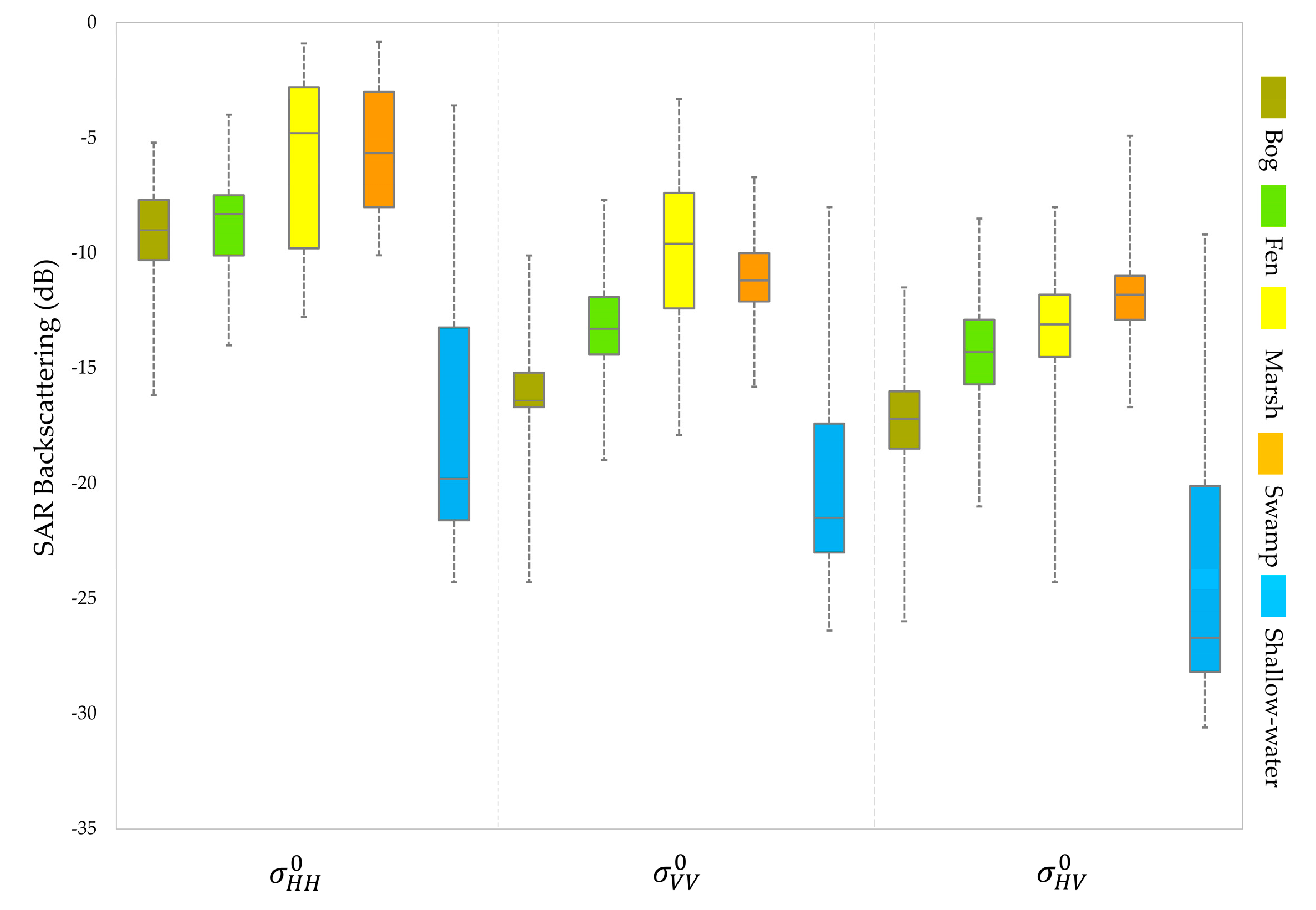
The spatial distribution of wetlands is of particular interest for the sustainable management of this important, productive ecosystem. In this study, the capability of full and simulated compact polarimetric (FP and CP) SAR data for wetland mapping was investigated in three pilot sites in Newfoundland and Labrador, Canada. A total of 13 FP and 22 simulated CP SAR features were extracted to identify the discrimination capability of these features between pairs of wetland classes both qualitatively, using backscattering analysis, and quantitatively, using the two-sample Kolmogorov-Smirnov (K-S) distance measurement. The most useful features were then identified and incorporated into the subsequent classification scheme.

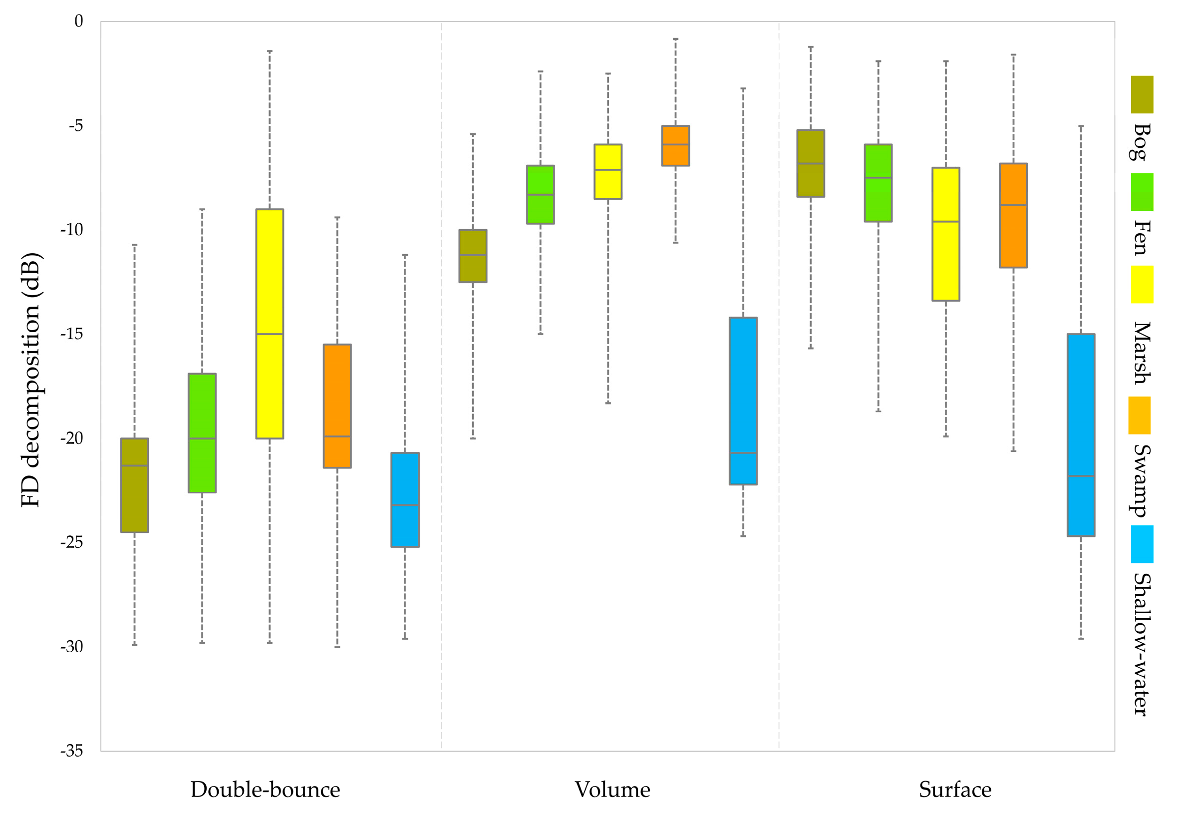
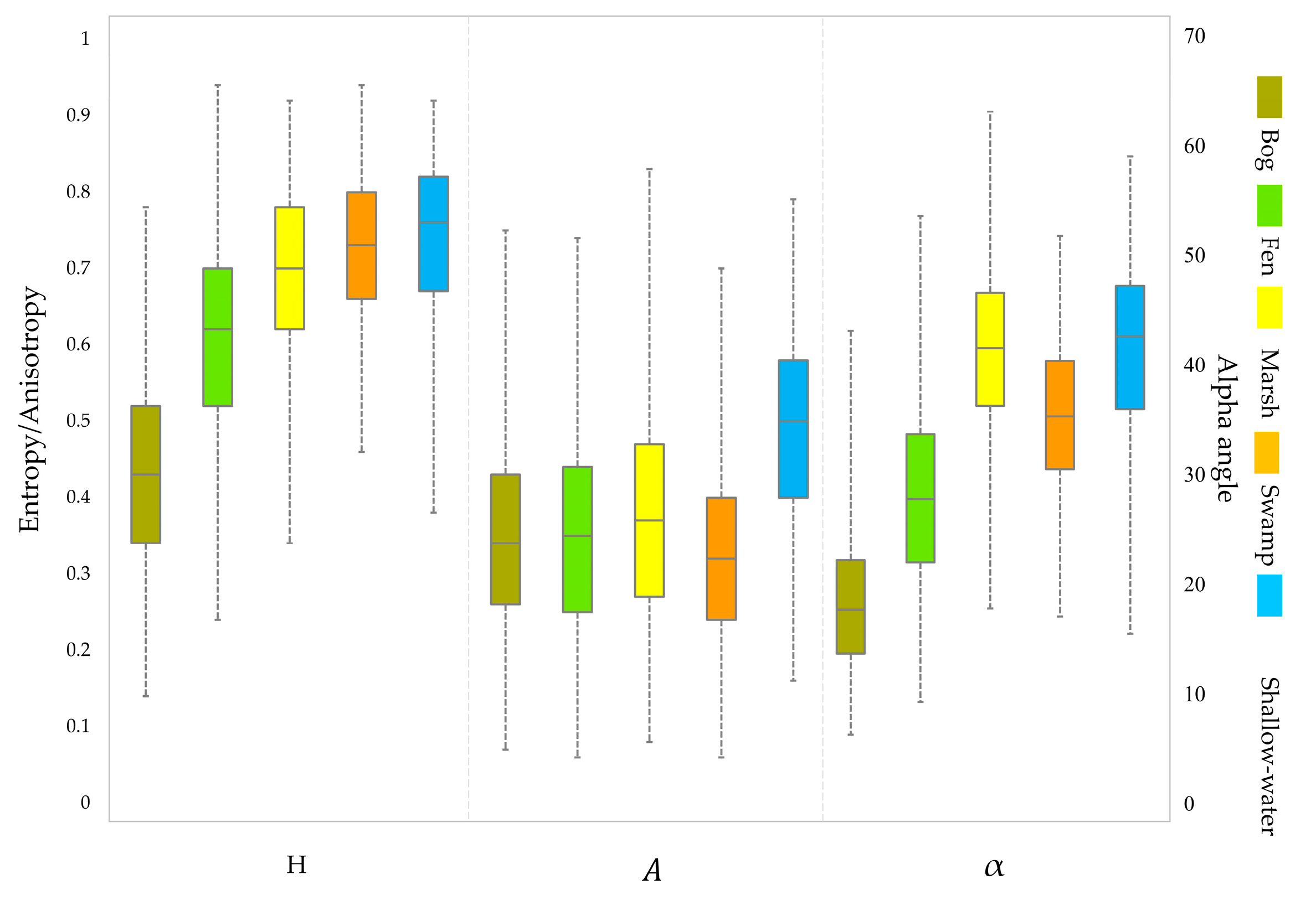
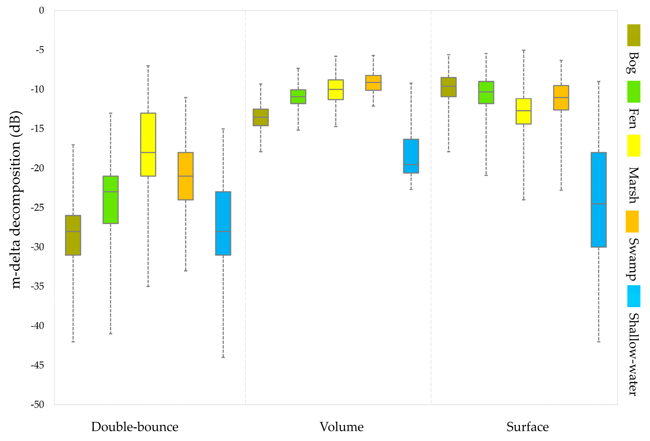
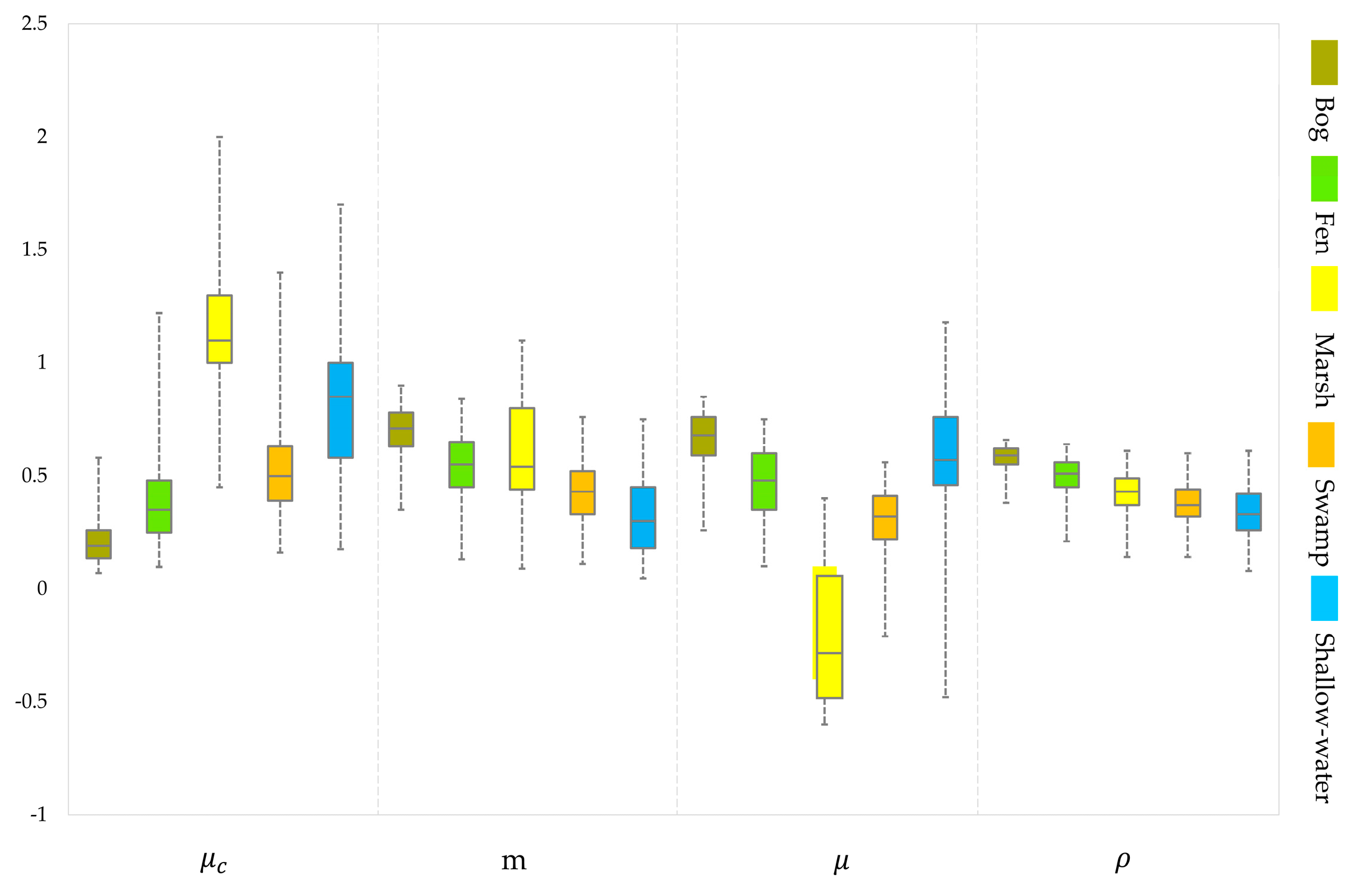
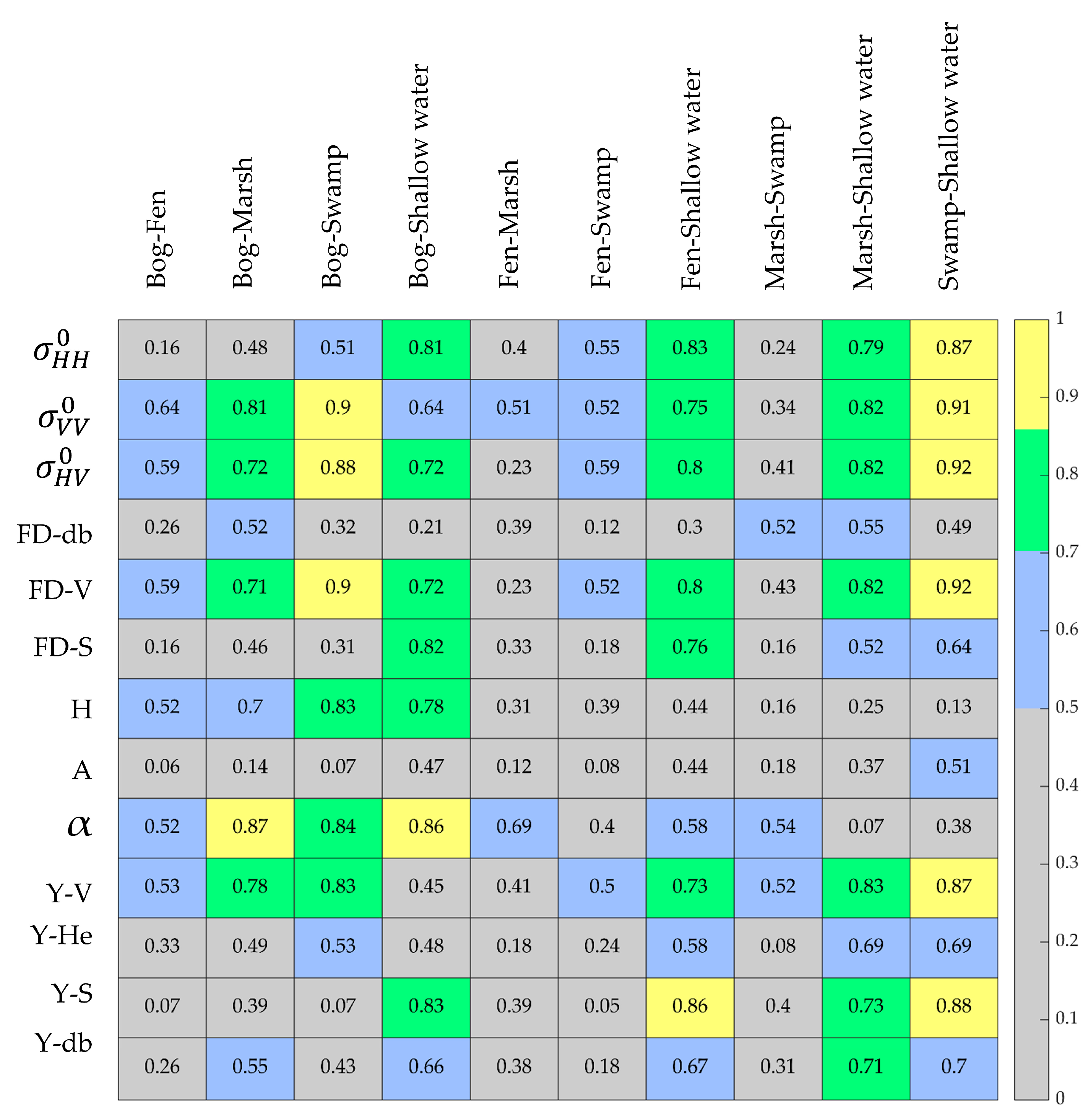
Among wetland classes, bog and shallow-water were found to be easily distinguished according to both the backscattering analysis and the K-S distance. Several features indicated either good or excellent separability between pairs of shallow-water-other classes and bog-other classes. Among FP features, backscattering intensity features, the Cloude-Pottier alpha angle, the volumetric components of the Freeman-Durden and Yamaguchi decompositions, as well as the surface scattering component of Yamaguchi decomposition were useful, as they indicated an excellent separability ($K-S>0.85$) between at least one pair of wetland classes. With regard to the CP SAR features, SAR backscattering coefficients, the first and last components of the Stokes vector, the circular polarization ratio, conformity coefficient, correlation coefficient, Shannon entropy, and both volume and surface scattering components of the m-chi and m-delta decompositions were useful features.

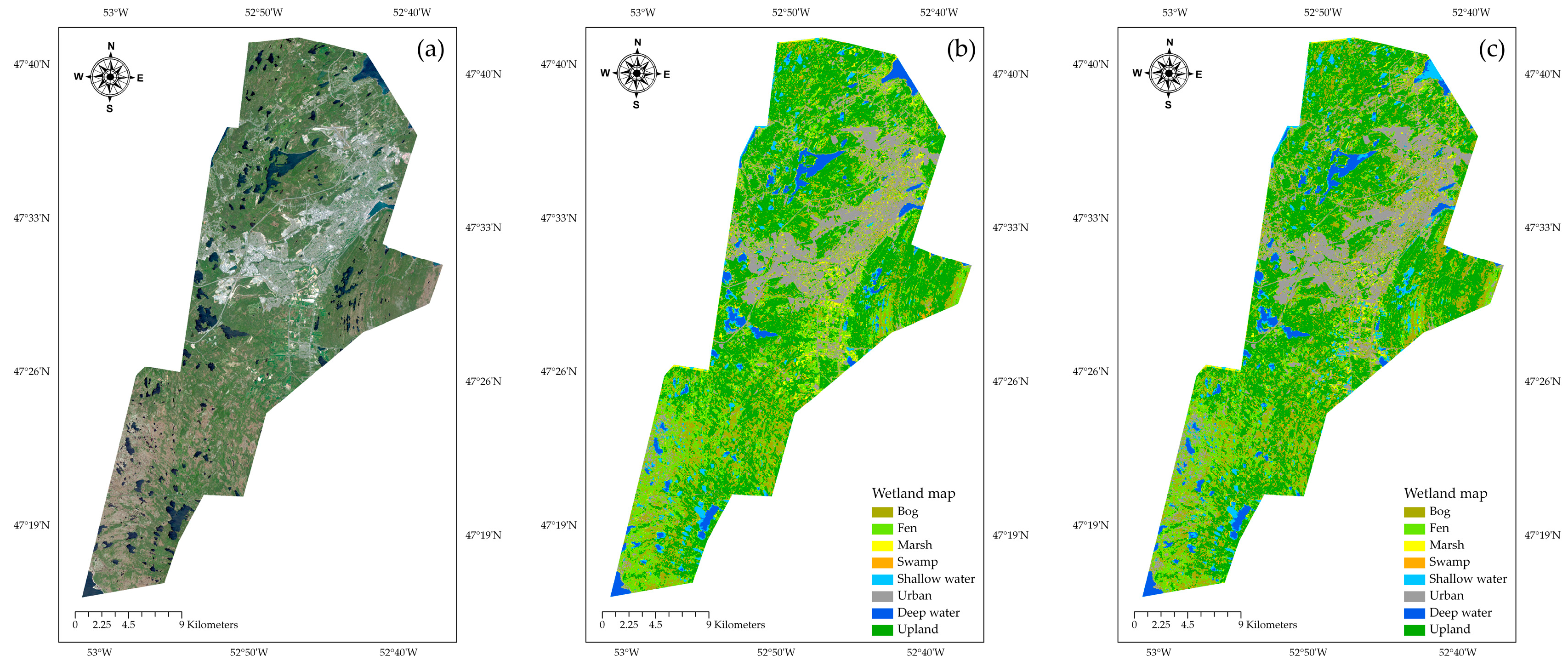
The overall accuracies of 87.89%, 80.67%, and 84.07% were obtained from the CP SAR data for the Avalon, Deer Lake, and Gros Morne study areas, respectively. The overall accuracies obtained from the FP SAR data were 90.73%, 84.75%, and 90.93% for the Avalon, Deer Lake, and Gros Morne study areas, respectively, which were higher than those of CP. Although the classification results demonstrated the superiority of FP SAR data compared to that of CP, the latter remains advantageous. This is because CP SAR data, which will be collected by RCM, will have a wider swath coverage and improved temporal resolution compared to those of RADARSAT-2. This is of great significance for efficiently mapping phenomena with highly dynamic natures (e.g., wetlands) on a large scale. Thus, the results of this research suggest that CP SAR data available on RCM hold great promise for discriminating conventional Canadian wetland classes. The analysis presented in this study contributes to further scientific research for wetland mapping and serves as a predecessor study for RCM, which will soon be the primary source of SAR observations in Canada.

References

1. Gardner, R.C.; Davidson, N.C. The ramsar convention. In Wetlands; Springer: Berlin, Germany, 2011; pp. 189–203. [Google Scholar]
2. Mitsch, W.J.; Bernal, B.; Nahlik, A.M.; Mander, Ü.; Zhang, L.; Anderson, C.J.; Jørgensen, S.E.; Brix, H. Wetlands, carbon, and climate change. Landsc. Ecol. 2013, 28, 583–597. [Google Scholar] [CrossRef]
3. Tiner, R.W.; Lang, M.W.; Klemas, V.V. Remote Sensing of Wetlands: Applications and Advances; CRC Press: Boca Raton, FL, USA, 2015; ISBN 1482237385. [Google Scholar]
4. Gallant, A.L. The challenges of remote monitoring of wetlands. Remote Sens. 2015, 7, 10938–10950. [Google Scholar] [CrossRef]
5. Mahdianpari, M.; Salehi, B.; Rezaee, M.; Mohammadimanesh, F.; Zhang, Y. Very Deep Convolutional Neural Networks for Complex Land Cover Mapping Using Multispectral Remote Sensing Imagery. Remote Sens. 2018, 10, 1119. [Google Scholar] [CrossRef]
6. Rezaee, M.; Mahdianpari, M.; Zhang, Y.; Salehi, B. Deep Convolutional Neural Network for Complex Wetland Classification Using Optical Remote Sensing Imagery. IEEE J. Sel. Top. Appl. Earth Obs. Remote Sens. 2018, 11, 3030–3039. [Google Scholar] [CrossRef]
7. Lee, J.-S.; Pottier, E. Polarimetric Radar Imaging: From Basics to Applications; CRC Press: Boca Raton, FL, USA, 2009; ISBN 1420054988. [Google Scholar]
8. Henderson, F.M.; Lewis, A.J. Radar detection of wetland ecosystems: A review. Int. J. Remote Sens. 2008, 29, 5809–5835. [Google Scholar] [CrossRef]
9. Brisco, B. Mapping and Monitoring Surface Water and Wetlands with Synthetic Aperture Radar. In Remote Sensing of Wetlands: Applications and Advances; CRC Press: New York, NY, USA, 2015; pp. 119–136. ISBN 1482237385. [Google Scholar]
10. Arnesen, A.S.; Silva, T.S.F.; Hess, L.L.; Novo, E.M.L.M.; Rudorff, C.M.; Chapman, B.D.; McDonald, K.C. Monitoring flood extent in the lower Amazon River floodplain using ALOS/PALSAR ScanSAR images. Remote Sens. Environ. 2013, 130, 51–61. [Google Scholar] [CrossRef]
11. Martinez, J.-M.; Le Toan, T. Mapping of flood dynamics and spatial distribution of vegetation in the Amazon floodplain using multitemporal SAR data. Remote Sens. Environ. 2007, 108, 209–223. [Google Scholar] [CrossRef]
12. Ward, D.P.; Petty, A.; Setterfield, S.A.; Douglas, M.M.; Ferdinands, K.; Hamilton, S.K.; Phinn, S. Floodplain inundation and vegetation dynamics in the Alligator Rivers region (Kakadu) of northern Australia assessed using optical and radar remote sensing. Remote Sens. Environ. 2014, 147, 43–55. [Google Scholar] [CrossRef]
13. Rebelo, L.-M. Eco-hydrological characterization of inland wetlands in Africa using L-band SAR. IEEE J. Sel. Top. Appl. Earth Obs. Remote Sens. 2010, 3, 554–559. [Google Scholar] [CrossRef]
14. Kasischke, E.S.; Bourgeau-Chavez, L.L. Monitoring South Florida wetlands using ERS-1 SAR imagery. Photogramm. Eng. Remote Sens. 1997, 63, 281–291. [Google Scholar]
15. Parmuchi, M.G.; Karszenbaum, H.; Kandus, P. Mapping wetlands using multi-temporal RADARSAT-1 data and a decision-based classifier. Can. J. Remote Sens. 2002, 28, 175–186. [Google Scholar] [CrossRef]
16. Touzi, R.; Deschamps, A.; Rother, G. Wetland characterization using polarimetric RADARSAT-2 capability. Can. J. Remote Sens. 2007, 33, S56–S67. [Google Scholar] [CrossRef]
17. Mahdianpari, M.; Salehi, B.; Mohammadimanesh, F.; Brisco, B.; Mahdavi, S.; Amani, M.; Granger, J.E. Fisher Linear Discriminant Analysis of coherency matrix for wetland classification using PolSAR imagery. Remote Sens. Environ. 2018, 206, 300–317. [Google Scholar] [CrossRef]
18. Cazals, C.; Rapinel, S.; Frison, P.-L.; Bonis, A.; Mercier, G.; Mallet, C.; Corgne, S.; Rudant, J.-P. Mapping and characterization of hydrological dynamics in a coastal marsh using high temporal resolution Sentinel-1A images. Remote Sens. 2016, 8, 570. [Google Scholar] [CrossRef]
19. Wohlfart, C.; Winkler, K.; Wendleder, A.; Roth, A. TerraSAR-X and Wetlands: A Review. Remote Sens. 2018, 10, 916. [Google Scholar] [CrossRef]
20. Mohammadimanesh, F.; Salehi, B.; Mahdianpari, M.; Motagh, M.; Brisco, B. An efficient feature optimization for wetland mapping by synergistic use of SAR intensity, interferometry, and polarimetry data. Int. J. Appl. Earth Obs. Geoinf. 2018, 73, 450–462. [Google Scholar] [CrossRef]
21. Ramsey III, E. Radar Remote Sensing of Wetlands. In Remote Sensing Change Detection: Environmental Monitoring Methods and Applications; Lunetta, R., Elvidge, C., Eds.; Ann Arbor Press: Chelsea, MA, USA, 1998; pp. 211–243. [Google Scholar]
22. Mohammadimanesh, F.; Salehi, B.; Mahdianpari, M.; Brisco, B.; Motagh, M. Wetland water level monitoring using interferometric synthetic aperture radar (InSAR): A review. Can. J. Remote Sens. 2018, 1–16. [Google Scholar] [CrossRef]
23. Kim, J.-W.; Lu, Z.; Jones, J.W.; Shum, C.K.; Lee, H.; Jia, Y. Monitoring Everglades freshwater marsh water level using L-band synthetic aperture radar backscatter. Remote Sens. Environ. 2014, 150, 66–81. [Google Scholar] [CrossRef]
24. Lu, Z.; Kwoun, O. Radarsat-1 and ERS InSAR analysis over southeastern coastal Louisiana: Implications for mapping water-level changes beneath swamp forests. IEEE Trans. Geosci. Remote Sens. 2008, 46, 2167–2184. [Google Scholar] [CrossRef]
25. Yuan, T.; Lee, H.; Jung, H.C. Toward estimating wetland water level changes based on hydrological sensitivity analysis of PALSAR backscattering coefficients over different vegetation fields. Remote Sens. 2015, 7, 3153–3183. [Google Scholar] [CrossRef]
26. Lee, H.; Yuan, T.; Jung, H.C.; Beighley, E. Mapping wetland water depths over the central Congo Basin using PALSAR ScanSAR, Envisat altimetry, and MODIS VCF data. Remote Sens. Environ. 2015, 159, 70–79. [Google Scholar] [CrossRef]
27. de Almeida Furtado, L.F.; Silva, T.S.F.; de Moraes Novo, E.M.L. Dual-season and full-polarimetric C band SAR assessment for vegetation mapping in the Amazon várzea wetlands. Remote Sens. Environ. 2016, 174, 212–222. [Google Scholar] [CrossRef]
28. Raney, R.K.; Cahill, J.T.S.; Patterson, G.; Bussey, D.B.J. The m-chi decomposition of hybrid dual-polarimetric radar data with application to lunar craters. J. Geophys. Res. Planets 2012, 117. [Google Scholar] [CrossRef]
29. Mahdianpari, M.; Salehi, B.; Mohammadimanesh, F.; Brisco, B. An Assessment of Simulated Compact Polarimetric SAR Data for Wetland Classification Using Random Forest Algorithm. Can. J. Remote Sens. 2017, 43, 468–484. [Google Scholar] [CrossRef]
30. Chen, Y.; He, X.; Wang, J.; Xiao, R. The influence of polarimetric parameters and an object-based approach on land cover classification in coastal wetlands. Remote Sens. 2014, 6, 12575–12592. [Google Scholar] [CrossRef]
31. van Beijma, S.; Comber, A.; Lamb, A. Random forest classification of salt marsh vegetation habitats using quad-polarimetric airborne SAR, elevation and optical RS data. Remote Sens. Environ. 2014, 149, 118–129. [Google Scholar] [CrossRef]
32. Lang, M.W.; Kasischke, E.S. Using C-band synthetic aperture radar data to monitor forested wetland hydrology in Maryland’s coastal plain, USA. IEEE Trans. Geosci. Remote Sens. 2008, 46, 535–546. [Google Scholar] [CrossRef]
33. Mahdianpari, M.; Salehi, B.; Mohammadimanesh, F.; Motagh, M. Random forest wetland classification using ALOS-2 L-band, RADARSAT-2 C-band, and TerraSAR-X imagery. ISPRS J. Photogramm. Remote Sens. 2017, 130, 13–31. [Google Scholar] [CrossRef]
34. Zhang, W.; Li, Z.; Chen, E.; Zhang, Y.; Yang, H.; Zhao, L.; Ji, Y. Compact Polarimetric Response of Rape (Brassica napus L.) at C-Band: Analysis and Growth Parameters Inversion. Remote Sens. 2017, 9, 591. [Google Scholar] [CrossRef]
35. Dabboor, M.; Montpetit, B.; Howell, S. Assessment of the High Resolution SAR Mode of the RADARSAT Constellation Mission for First Year Ice and Multiyear Ice Characterization. Remote Sens. 2018, 10, 594. [Google Scholar] [CrossRef]
36. Torres, R.; Snoeij, P.; Geudtner, D.; Bibby, D.; Davidson, M.; Attema, E.; Potin, P.; Rommen, B.; Floury, N.; Brown, M. GMES Sentinel-1 mission. Remote Sens. Environ. 2012, 120, 9–24. [Google Scholar] [CrossRef]
37. Aschbacher, J.; Milagro-Pérez, M.P. The European Earth monitoring (GMES) programme: Status and perspectives. Remote Sens. Environ. 2012, 120, 3–8. [Google Scholar] [CrossRef]
38. Mahdianpari, M.; Salehi, B.; Mohammadimanesh, F.; Homayouni, S.; Gill, E. The First Wetland Inventory Map of Newfoundland at a Spatial Resolution of 10 m Using Sentinel-1 and Sentinel-2 Data on the Google Earth Engine Cloud Computing Platform. Remote Sens. 2019, 11, 43. [Google Scholar] [CrossRef]
39. Tan, W.; Li, J.; Xu, L.; Chapman, M.A. Semiautomated Segmentation of Sentinel-1 SAR Imagery for Mapping Sea Ice in Labrador Coast. IEEE J. Sel. Top. Appl. Earth Obs. Remote Sens. 2018, 11, 1419–1432. [Google Scholar] [CrossRef]
40. Van Tricht, K.; Gobin, A.; Gilliams, S.; Piccard, I. Synergistic use of radar Sentinel-1 and optical Sentinel-2 imagery for crop mapping: a case study for Belgium. Remote Sens. 2018, 10, 1642. [Google Scholar] [CrossRef]
41. Espeseth, M.M.; Brekke, C.; Johansson, A.M. Assessment of RISAT-1 and Radarsat-2 for sea ice observations from a hybrid-polarity perspective. Remote Sens. 2017, 9, 1088. [Google Scholar] [CrossRef]
42. Raney, R.K. Hybrid-polarity SAR architecture. IEEE Trans. Geosci. Remote Sens. 2007, 45, 3397–3404. [Google Scholar] [CrossRef]
43. Thompson, A.A. Overview of the RADARSAT constellation mission. Can. J. Remote Sens. 2015, 41, 401–407. [Google Scholar] [CrossRef]
44. Banks, S.; Millard, K.; Behnamian, A.; White, L.; Ullmann, T.; Charbonneau, F.; Chen, Z.; Wang, H.; Pasher, J.; Duffe, J. Contributions of Actual and Simulated Satellite SAR Data for Substrate Type Differentiation and Shoreline Mapping in the Canadian Arctic. Remote Sens. 2017, 9, 1206. [Google Scholar] [CrossRef]
45. Charbonneau, F.J.; Brisco, B.; Raney, R.K.; McNairn, H.; Liu, C.; Vachon, P.W.; Shang, J.; DeAbreu, R.; Champagne, C.; Merzouki, A. Compact polarimetry overview and applications assessment. Can. J. Remote Sens. 2010, 36, S298–S315. [Google Scholar] [CrossRef]
46. Singha, S.; Ressel, R. Arctic sea ice characterization using RISAT-1 compact-pol SAR imagery and feature evaluation: A case study over Northeast Greenland. IEEE J. Sel. Top. Appl. Earth Obs. Remote Sens. 2017, 10, 3504–3514. [Google Scholar] [CrossRef]
47. Dabboor, M.; Geldsetzer, T. Towards sea ice classification using simulated RADARSAT Constellation Mission compact polarimetric SAR imagery. Remote Sens. Environ. 2014, 140, 189–195. [Google Scholar] [CrossRef]
48. Brisco, B.; Li, K.; Tedford, B.; Charbonneau, F.; Yun, S.; Murnaghan, K. Compact polarimetry assessment for rice and wetland mapping. Int. J. Remote Sens. 2013, 34, 1949–1964. [Google Scholar] [CrossRef]
49. White, L.; Millard, K.; Banks, S.; Richardson, M.; Pasher, J.; Duffe, J. Moving to the RADARSAT constellation mission: Comparing synthesized compact polarimetry and dual polarimetry data with fully polarimetric RADARSAT-2 data for image classification of peatlands. Remote Sens. 2017, 9, 573. [Google Scholar] [CrossRef]
50. Marshall, I.B.; Schut, P.; Ballard, M. A National Ecological Framework for Canada. Available online: http://sis.agr.gc.ca/cansis/publications/manuals/1996/A42-65-1996-national-ecological-framework.pdf (accessed on 1 January 2019).
51. Mohammadimanesh, F.; Salehi, B.; Mahdianpari, M.; Brisco, B.; Motagh, M. Multi-temporal, multi-frequency, and multi-polarization coherence and SAR backscatter analysis of wetlands. ISPRS J. Photogramm. Remote Sens. 2018, 142, 78–93. [Google Scholar] [CrossRef]
52. Kim, S.-W.; Wdowinski, S.; Amelung, F.; Dixon, T.H.; Won, J.-S. Interferometric coherence analysis of the Everglades wetlands, South Florida. IEEE Trans. Geosci. Remote Sens. 2013, 51, 5210–5224. [Google Scholar] [CrossRef]
53. Mahdianpari, M.; Salehi, B.; Mohammadimanesh, F. The Effect of PolSAR Image De-speckling on Wetland Classification: Introducing a New Adaptive Method. Can. J. Remote Sens. 2017, 43, 485–503. [Google Scholar] [CrossRef]
54. Toutin, T.; Cheng, P. Demystification of IKONOS. Earth Obs. Mag. 2000, 9, 17–21. [Google Scholar]
55. Zhang, L.; He, X.; Balz, T.; Wei, X.; Liao, M. Rational function modeling for spaceborne SAR datasets. ISPRS J. Photogramm. Remote Sens. 2011, 66, 133–145. [Google Scholar] [CrossRef]
56. Baghdadi, N.; Bernier, M.; Gauthier, R.; Neeson, I. Evaluation of C-band SAR data for wetlands mapping. Int. J. Remote Sens. 2001, 22, 71–88. [Google Scholar] [CrossRef]
57. Paloscia, S.; Pettinato, S.; Santi, E.; Notarnicola, C.; Pasolli, L.; Reppucci, A. Soil moisture mapping using Sentinel-1 images: Algorithm and preliminary validation. Remote Sens. Environ. 2013, 134, 234–248. [Google Scholar] [CrossRef]
58. Gao, Q.; Zribi, M.; Escorihuela, M.J.; Baghdadi, N. Synergetic use of Sentinel-1 and Sentinel-2 data for soil moisture mapping at 100 m resolution. Sensors 2017, 17, 1966. [Google Scholar] [CrossRef] [PubMed]
59. Cloude, S.R.; Pottier, E. An entropy based classification scheme for land applications of polarimetric SAR. IEEE Trans. Geosci. Remote Sens. 1997, 35, 68–78. [Google Scholar] [CrossRef]
60. Freeman, A.; Durden, S.L. A three-component scattering model for polarimetric SAR data. IEEE Trans. Geosci. Remote Sens. 1998, 36, 963–973. [Google Scholar] [CrossRef]
61. Yamaguchi, Y.; Moriyama, T.; Ishido, M.; Yamada, H. Four-component scattering model for polarimetric SAR image decomposition. IEEE Trans. Geosci. Remote Sens. 2005, 43, 1699–1706. [Google Scholar] [CrossRef]
62. Ballester-Berman, J.D.; Lopez-Sanchez, J.M. Time series of hybrid-polarity parameters over agricultural crops. IEEE Geosci. Remote Sens. Lett. 2012, 9, 139–143. [Google Scholar] [CrossRef]
63. Cloude, S.R.; Goodenough, D.G.; Chen, H. Compact decomposition theory. IEEE Geosci. Remote Sens. Lett. 2012, 9, 28–32. [Google Scholar] [CrossRef]
64. Truong-Loi, M.-L.; Freeman, A.; Dubois-Fernandez, P.C.; Pottier, E. Estimation of soil moisture and Faraday rotation from bare surfaces using compact polarimetry. IEEE Trans. Geosci. Remote Sens. 2009, 47, 3608–3615. [Google Scholar] [CrossRef]
65. Marechal, C.; Pottier, E.; Hubert-Moy, L.; Rapinel, S. One year wetland survey investigations from quad-pol RADARSAT-2 time-series SAR images. Can. J. Remote Sens. 2012, 38, 240–252. [Google Scholar] [CrossRef]
66. Geldsetzer, T.; Arkett, M.; Zagon, T.; Charbonneau, F.; Yackel, J.J.; Scharien, R.K. All-season compact-polarimetry C-band SAR observations of sea ice. Can. J. Remote Sens. 2015, 41, 485–504. [Google Scholar] [CrossRef]
67. Massey, F.J., Jr. The Kolmogorov-Smirnov test for goodness of fit. J. Am. Statist. Assoc. 1951, 46, 68–78. [Google Scholar] [CrossRef]
68. Blaschke, T. Object based image analysis for remote sensing. ISPRS J. Photogramm. Remote Sens. 2010, 65, 2–16. [Google Scholar] [CrossRef]
69. Breiman, L. Random forests. Mach. Learn. 2001, 45, 5–32. [Google Scholar] [CrossRef]
70. Belgiu, M.; Drăguţ, L. Random forest in remote sensing: A review of applications and future directions. ISPRS J. Photogramm. Remote Sens. 2016, 114, 24–31. [Google Scholar] [CrossRef]
71. Mahdianpari, M.; Salehi, B.; Mohammadimanesh, F.; Larsen, G.; Peddle, D.R. Mapping land-based oil spills using high spatial resolution unmanned aerial vehicle imagery and electromagnetic induction survey data. J. Appl. Remote Sens. 2018, 12, 036015. [Google Scholar] [CrossRef]
72. Mohammadimanesh, F.; Salehi, B.; Mahdianpari, M.; English, J.; Chamberland, J.; Alasset, P.-J. Monitoring surface changes in discontinuous permafrost terrain using small baseline SAR interferometry, object-based classification, and geological features: a case study from Mayo, Yukon Territory, Canada. GISci. Remote Sens. 2018, 1–26. [Google Scholar] [CrossRef]
73. Congalton, R.G. A review of assessing the accuracy of classifications of remotely sensed data. Remote Sens. Environ. 1991, 37, 35–46. [Google Scholar] [CrossRef]
74. Dingle Robertson, L.; King, D.J.; Davies, C. Object-based image analysis of optical and radar variables for wetland evaluation. Int. J. Remote Sens. 2015, 36, 5811–5841. [Google Scholar] [CrossRef]
75. McNairn, H.; Shang, J.; Jiao, X.; Champagne, C. The contribution of ALOS PALSAR multipolarization and polarimetric data to crop classification. IEEE Trans. Geosci. Remote Sens. 2009, 47, 3981–3992. [Google Scholar] [CrossRef]
76. White, L.; Landon, A.; Dabboor, M.; Pratt, A.; Brisco, B. Mapping and monitoring flooded vegetation and soil moisture using simulated compact polarimetry. In Proceedings of the Geoscience and Remote Sensing Symposium (IGARSS), Quebec City, QC, Canada, 13–18 July 2014; pp. 1568–1571. [Google Scholar]
77. Dabboor, M.; Brisco, B. Wetland Monitoring Using Synthetic Aperture Radar Imagery. In Wetlands; IntechOpen: London, UK, 2018. [Google Scholar]
Figure 1. The red polygons illustrate the geographic location of the three study areas.
Remotesensing 11 00516 g001
Figure 2. Examples of land cover classes in the Avalon study area, including (a) bog, (b) fen, (c) marsh, (d) swamp, (e) shallow water, (f) urban, (g) deep water, and (h) upland.
Remotesensing 11 00516 g002
Figure 3. Box-and-whisker plots demonstrating the distribution of the SAR backscattering coefficients of FP SAR data for wetland classes obtained from the pixel values of the training data set. Note that the horizontal bars within boxes indicate median values, boxes illustrate the lower and upper quartiles, and whiskers range from minimum to maximum values.
Remotesensing 11 00516 g003
Figure 4. Box-and-whisker plots for extracted features from the Freeman-Durden decomposition for wetland classes obtained from the pixel values of the training data set.
Remotesensing 11 00516 g004
Figure 5. Box-and-whisker plots for extracted features from the Cloude-Pottier decomposition for wetland classes obtained from the pixel values of the training data set. Note: H: entropy, A: anisotropy, and α: alpha angle.
Remotesensing 11 00516 g005
Figure 6. Box-and-whisker plots demonstrating the distribution of the SAR backscattering coefficients of CP SAR data for wetland classes obtained from the pixel values of the training data set. The red horizontal line highlights the nominal NESZ (-24 dB) of the RCM medium resolution mode.
Remotesensing 11 00516 g006
Figure 7. Box-and-whisker plots for extracted features from the m-delta decomposition for wetland classes obtained from the pixel values of the training data set.
Remotesensing 11 00516 g007
Figure 8. Box-and-whisker plots for extracted features from the CP SAR data for wetland classes obtained from pixel values of the training data set. Note: µc: circular polarization ratio, m: degree of polarization, µ: conformity coefficient, and ρ: correlation coefficient.
Remotesensing 11 00516 g008
Figure 9. K-S distances between pairs of wetland classes using the extracted features from FP SAR data. Note that gray, blue, green, and yellow indicate poor, some, good, and excellent separability, respectively.
Remotesensing 11 00516 g009
Figure 10. K-S distances between pairs of wetland classes using the features extracted from CP SAR data. See Table 3 for parameter description.
Remotesensing 11 00516 g010
Figure 11. (a) A true color composite of RapidEye optical imagery (bands 3, 2, and 1) acquire on June 18, 2015. The classification maps of the Avalon study area obtained from (b) FP (OA: 90.73%, K: 0.88) and (c) simulated CP SAR data (OA: 87.89%, K: 0.85).
Remotesensing 11 00516 g011
Figure 12. (a) A true color composite of RapidEye optical imagery (bands 3, 2, and 1) acquire on June 18, 2015. The classification maps of the Deer Lake study area obtained from (b) FP (OA: 84.75%, K: 0.81) and (c) simulated CP SAR data (OA: 80.67%, K: 0.77).
Remotesensing 11 00516 g012
Figure 13. (a) A true color composite of RapidEye optical imagery (bands 3, 2, and 1) acquire on June 18, 2015. The classification maps of the Gros Morne study area obtained from (b) FP (OA: 90.93%, K: 0.88) and (c) simulated CP SAR data (OA: 84.07%, K: 0.80).
Remotesensing 11 00516 g013