Identification of Dust Sources in a Saharan Dust Hot-Spot and Their Implementation in a Dust-Emission Model


Leibniz Institute for Tropospheric Research, 04315 Leipzig, Germany
*
Author to whom correspondence should be addressed.
Remote Sens. 2019, 11(1), 4; https://doi.org/10.3390/rs11010004
Submission received: 20 November 2018
/
Revised: 14 December 2018
/
Accepted: 18 December 2018
/
Published: 20 December 2018
(This article belongs to the Special Issue Remote Sensing in Support of Aeolian Research)
Abstract
:Although mineral dust plays a key role in the Earth’s climate system and in climate and weather prediction, models still have difficulties in predicting the amount and distribution of mineral dust in the atmosphere. One reason for this is the limited understanding of the distribution of dust sources and their behavior with respect to their spatiotemporal variability in activity. For a better estimation of the atmospheric dust load, this paper presents an approach to localize dust sources and thereby estimate the sediment supply for a study area centered on the Aïr Massif in Niger with a north–south extent of 16–22 N and an east–west extent of 4–12 E. This approach uses optical Sentinel-2 data at visible and near infrared wavelengths together with HydroSHEDS flow accumulation data to localize ephemeral riverbeds. Visible channels from Sentinel-2 data are used to detect sand sheets and dunes. The identified sediment supply map was compared to the dust source activation frequency derived from the analysis of Desert-Dust-RGB imagery from the Meteosat Second Generation series of satellites. This comparison reveals the strong connection between dust activity, prevailing meteorology and sediment supply. In a second step, the sediment supply information was implemented in a dust-emission model. The simulated emission flux shows how much the model results benefit from the updated sediment supply information in localizing the main dust sources and in retrieving the seasonality of dust activity from these sources. The described approach to characterize dust sources can be implemented in other regional model studies, or even globally, and can thereby help to get a more accurate picture of dust source distribution and a more realistic estimation of the atmospheric dust load.
1. Introduction
The World’s most important dust sources are located in the Sahara. It has been estimated that 55% of the global dust emissions originate from the North African desert [1]. The most active dust source in the Sahara is the Bodélé depression in Chad, which is considered to produce half of the mineral aerosols emitted from the Sahara [2]. Whereas the Bodélé depression has been subject to a number of on-site measurement, model and remote sensing investigations (e.g., [2,3,4]), the characteristics of other Saharan dust sources remain less understood, not only in their spatial distribution but also in the understanding of their temporal variability in activity from daily to seasonal [5] as well as inter-annual scales [6].
For the analysis of dust sources and their impact on the Earth system, it is crucial to know how the sources are distributed and how variably active they are. However, dust source mapping is far from being a trivial task. Most dust source activity takes place along the so-called dust belt, which includes the World’s most remote areas in the Sahara, the Middle East, Central Asia and China [7], where the population density is low and so is observational data availability. This is why the most widely-known attempts to map the sources of airborne dust are based on remote sensing products that replicate the atmospheric dust load [1,7,8,9,10,11,12]. This approach is based on the premise that dust sources are located where the atmospheric dust load is increased. However, polar-orbiting satellites have the disadvantage of very few or even no overpass per day, leading to a possible mislocalization of the dust sources when overpass time and time of dust source activation diverge. A more accurate source determination can be achieved using data from the geostationary Meteosat Second Generation (MSG) satellites, which capture the Sahara and Arabian Peninsula at a temporal resolution of 15 min. The high temporal resolution enables the location of the origin of dust plumes in a more precise way. The spatial resolution of 3 km at nadir allows assigning the origin of a dust plume to a specific landscape. An analysis of an MSG-based dust product published by Schepanski et al. [13] reveals that active dust sources in the Sahara tend to be found in rugged and complex terrain around the mountain ranges of the Saharan desert. This raises some fundamental research questions: What surface features are found in these regions that hold sediments in the size range suitable for wind erosion? What are the processes that recharge these sources with fresh sediments in the quantity to enable particle mobilization over years, decades and centuries?
Several field studies find that one important source type are sediments accumulated by surficial water runoff, so-called alluvial sediments. For example, a long-term measurement campaign conducted by Reheis and Kihl [14] in the southwestern US between 1984 and 1989 shows an increased emission flux derived from these sources, especially subsequent to strong precipitation and inundation events. In the framework of the Fennec campaign in 2011 [15], an airborne campaign focusing on dust emission in Mauritania determines dry river valleys as the sources of mineral dust [16]. These findings are underlined by larger scale satellite-based studies in many desert regions, such as in the southwestern US [12,17,18], southern Africa [19,20,21] and the Sahara and Middle East region [10,22,23], which stress the role that hydrological features play in the total atmospheric dust load in different regions of the globe. The major study analyzing dust sources on a global scale is without doubt the analysis of MODIS Deep Blue dust information in comparison with surface information undertaken by Ginoux et al. [1]. This study suggests that 31 % of the global dust is emitted from hydrological sources such as ephemeral water bodies. For North Africa, this number rises to 92% of total dust emission being derived from hydrologic sources.
Due to the complexity of these features, their dependency on the local geomorphology and meteorology and their small size (e.g., the basins of ephemeral rivers of some tens or hundreds of meters up to a few kilometers in width) there is a strong discrepancy between their importance and their representation in dust emission models. This leads to an underestimation of sediment supply in the models, which can partly explain the mismatch between the observed and simulated atmospheric dust load and the strong divergence of dust loading retrieved for different dust models [16,24,25].
For a more successful representation of alluvial sources in dust models, not only a better understanding of the processes behind the emission is needed, but also methods to localize these important features on larger scales are required. One approach that intends to extract ephemeral river basins from satellite images was published by Parajuli and Zender [26], where optical remote sensing data of the blue light is combined with digital elevation information. We adapted and extended this approach and tested our method for a study area in the Sahara, for which a sediment supply map was created from the determination of fluvial systems and dunes. This information was compared to the dust source activation frequency derived from MSG’s Desert-Dust-RGB product to connect the extracted source features to dust emission. The identified sources were then implemented in a dust emission model to analyze whether sediment supply information can produce more accurate modeling results.
The overall scope of the manuscript is to identify how important the small-scale alluvial sediment layers are for the local and regional atmospheric dust load and how we can implement these sources in a model to improve the calculated dust emission.
2. Study Area: Meteorological and Geomorphical Setting
The Aïr Massif in Niger is a known dust hot-spot in the Sahara [1,7,11], and was hence chosen as the study area for this research. Figure 1 depicts the location of the study area in North Africa and outlines the main meteorological features affecting the area.
2.1. Main Meteorological Features of the Study Area
The two key large scale meteorological phenomena that influence the study area, i.e., the West African Monsoon (WAM) during boreal summer and the Harmattan trade winds during northern hemispheric winter, are sketched out in Figure 1. These two features lead to a daily and annual cycle of wind and precipitation regimes in the region.
Especially the wind speed distribution is crucial for dust emission: only when a certain threshold velocity is exceeded can particles be entrained into the atmosphere [27]. This threshold velocity is dependent on a number of surface characteristics such as the size of erodible aggregates, soil crusts and vegetation cover. Two key processes that are known to lead to an increase in surface wind speed and increased dust emission are found in the area: (1) the breakdown of the nocturnal low level jet in the morning hours during both the Harmattan and WAM phases [3,5,28,29], to which more than half of the dust events in the Sahara can be connected [5]; and (2) mesoscale convective systems (MCS), mainly connected to the WAM [30,31]. These systems are less frequent but, due to strong outflow winds, can provoke enormous dust events in the size of up to hundreds of kilometers called haboobs (e.g., [30,32]).
2.2. Geomorphology of the Study Area
The MCS that occur during the WAM phase not only bring increased wind velocities, but the high moisture content of the monsoon triggered cyclones is further able to provoke extreme precipitation events in the study area, where throughout the rest of the year arid to hyperarid conditions prevail. These rain events lead to surface runoff of precipitated water and, associated to this, the erosion, transport and finally the accumulation of sediments at the foothills of mountains, within ephemeral river basins, alluvial fans or flood plains. During extreme precipitation events, flash floods can occur, washing down enormous amounts of fresh material forming new sediment layers at the mountain bases (e.g., [33]). This leads to a complex surface sediment structure, especially southwest of the mountain range which is most affected by the WAM: while the massif itself consists of metamorphic rocks with granite intrusions, the southwest is characterized by compressed and loose sediment layers of several quaternary sedimentation phases [34,35] covered by fresh sediment layers accumulated by recent monsoon precipitation [36].
These recently accumulated and quaternary fine alluvial sediments are considered as important sources of dust in the study area as they contain particles in a size range that is prone to wind erosion [1,11,16,17,19]. Not without reason is the area around the Aïr Massif proven to be one of the most active dust sources in the Sahara [1,7,13], a fact that Prospero et al. [7] and Ginoux et al. [1] clearly connected to the system of ephemeral rivers and streams, which drain the Aïr Massif on its southwestern edge during the WAM phases.
Considering the diverse meteorological patterns that influence the area together with the ruggedness of the terrain, which leads to a complex geomorphology, the Aïr Massif offers a unique setting to study the connection between wind, precipitation, and the distribution and formation of fresh sediment layers and dust emission.
3. Data
3.1. MSG-3 and the Desert-Dust-RGB Product
Since 2004, the Meteosat Second Generation satellite series deliver data on the atmosphere for Europe, Africa and the Arabian Peninsula from the geostationary position at 0 N/0 E. Mounted on MSG-3 (also known as Meteosat-10), the current European weather observation satellite, is the Spinning Enhanced Visible and InfraRed Imager (SEVIRI), which captures the full disc with a temporal resolution of 15 min [37]. SEVIRI’s eleven spectral bands cover visible to infrared (IR) wavelength ranges with a nadir-resolution of 3 km [37] and a resolution of around 4.5 km in the study area. Due to its location and its spectral capabilities, the MSG Desert-Dust-RGB product is perfectly suitable not only for weather prediction and for the observation of short term weather phenomena in Europe, but also to monitor atmospheric processes of the Sahara in general and dust emission in particular [11,38,39]. For dust monitoring, EUMETSAT offers a Desert-Dust-RGB product [40], a composite based on the brightness temperature (BT) and brightness temperature differences of three SEVIRI infrared bands ( , , and ). On this composite, dust plumes appear in pink color and are, at least with some experience, easy to spot, especially in cloud-free conditions. Due to the usage only of IR-bands, this method is applicable during day and night time.
3.2. Sentinel-2 Data and Preprocessing
For the analysis of the surface structure and the location of potential dust sources, spaceborne data of ESA’s Sentinel-2 satellite were used. The Multispectral Instrument (MSI) aboard Sentinel-2 samples for 13 spectral bands at a resolution of 10–60 m, and covers the visible, near infrared (NIR) and short wave infrared (SWIR) wavelengths [41]. Sentinel-2 level 1C data are made available through ESA’s scientific data hub Copernicus (https://scihub.copernicus.eu/) as geoprojected top-of-atmosphere (TOA) reflectances.
To cover the study area, four Sentinel-2 images are needed. Table 1 shows details of the sensing dates and row numbers of the four images chosen for the analysis. All of them are cloud free and were obtained in May or June 2016 and hence before the onset of the WAM. This was done to ensure that the vegetation cover is at its annual minimum.
The four images were corrected for atmospheric influences using the ESA-supported third-party command-line plugin Sen2Cor. During the atmospheric correction, the level 1C TOA data were transformed into bottom-of-atmosphere (BOA) reflectance using a large database of look-up tables for a wide range of atmospheric conditions, solar geometries, and ground elevations. The main steps of the correction process include the estimation of aerosol optical thickness and water vapor and the removal of cirrus clouds (for more details, see [42]). After the correction process, the cloud-, aerosol-, and water vapor-corrected bands were resampled to a resolution of 40 m.
3.3. Vegetation
Vegetation cover plays an important role in topsoil stabilization and therefore in suppressing particle mobilization and dust emission [27,43]. Hence, it is an important factor to consider when analyzing and characterizing dust sources and when parametrizing dust emission.
A tool to monitor vegetation cover and its changes is the normalized difference vegetation index (NDVI) derived from the ratio of the red and NIR reflectance data, as depicted in Equation (1).
The NDVI shows the distribution of healthy vegetation and is sufficiently robust to reflect seasonal and inter-annual changes in vegetation cover. Due to this ratio, the main advantage of the NDVI compared to other vegetation indices is its reduction of noise, which is present throughout a larger part of the reflectance spectra, e.g., atmospheric, topographic or sensor geometry based effects [44]. In this study, the MODIS/Aqua monthly vegetation product MYD13A3 V6 with 1 km × 1 km resolution was used [45]. The global product is based on the best available pixel in means of low cloud cover, low view angle, and highest NDVI value, of all acquisitions of a 16-day period. The suitability of this product for semi-arid regions was proven, for example, by Fenshold et al. [46].
3.4. ECMWF Forecast Wind
To drive the dust-emission model, the wind field derived from the European Centre for Medium Range Weather Forecast (ECMWF, Reading, UK) forecast model was used. The winds at 10 m height (lowest model level) in a temporal resolution of 1 h and a grid spacing of 0.1 × 0.1 offer the best possible estimate of dust relevant winds in the study area.
4. Methods
4.1. Determination of Dust Activity and Dust Hot-Spots
Dust activity within the study area was determined by applying the back-tracking method introduced by Schepanski et al. [11] on the Desert-Dust-RGB images derived from MSG-3. The method takes advantage of the high temporal resolution of the product. Dust plumes spotted on the dust product can manually be traced back to their origin by going through the 15-min composites in reverse. Thereby, the sources of dust plumes are localized and mapped. This manual approach was used, since, due to the complex sensitivities of the thermal IR dust signature regarding dust optical properties, surface emissivity and atmospheric conditions (e.g., [39]), the design of an automatic retrieval algorithm is challenging. The described method was applied for a four-year period from 1 January 2013 to 31 December 2016 for the study area centered on the Aïr Massif. Each dust plume that occurred during this time period was traced back to its origin and mapped on an overlaying, regular grid. The grid spacing was 0.5 × 0.5 covering the area from 2 E to 13 E and from 14.5 N to 22 N. The result is a dust source activation frequency (DSAF) map that shows how often each grid cell was active during the four years. This allowed determining areas of high dust emission activity and to monitor not only the total number of dust events from each grid cell, but also their seasonal activity.
4.2. Sediment Supply Map
To simulate the dust emission flux, sediment supply information was extracted from the four preprocessed Sentinel-2 images. To reduce the complexity of the surface, we focused on two dominant dust source types frequently discussed in the literature, i.e., the alluvial sediments (e.g., [1,14,17,23,26,47]), also discussed in the Introduction, and sand dunes and sand sheets that are receiving increasing attention in recent years [17,48,49]. The following sections describe the strategies for the extraction of these surfaces from the optical remote sensing data and their combination into a sediment supply map (SSM), which is directly included in the dust-emission modeling approach.
4.2.1. Alluvial Sediment Map
Parajuli and Zender [26] developed an approach to detect sediments accumulated by flowing water, taking into account the spectral characteristics of a surface together with the geomorphology of the landscape. In this study, we paper a similar but improved approach to localize alluvial sediments in the study area more accurately and in higher resolution. The approach includes two levels of information, the geomorphic erodibility introduced by Zender et al. [50] based on digital elevation information and spectral information of visible and infrared wavelengths derived from the Sentinel-2 satellite.
The flow chart in Figure 2A shows the main steps to derive the alluvial fines map (AFM). The geomorphic erodibility takes into account the position of each pixel in the local digital elevation model (DEM), from which the respective upstream area is derived. It assumes that a larger upstream area allows for a stronger accumulation of sediments in the respective pixel, leading to a theoretically increased amount of available sediments proportional to the upstream area. Similar to Parajuli and Zender [26], we used the HydroSHEDS flow accumulation (FA) dataset [51]. This dataset is based on the DEM derived from NASA’s Shuttle Radar Topography Mission (SRTM) and gives the number of upstream pixels for each pixel of the dataset. Hence, it gives information on the location of each pixel within the regional catchment area. The dataset was used in its highest resolution of 15" (approx. 31 m).
The left leg of Figure 2A shows the processing steps from the original FA data towards the normalized and compressed FAlog100 dataset: first, the global FA dataset was subsetted to the extent of the Sentinel-2 mosaic. The resulting image pixels hold values between 0 for relative mountain ridges compared to the surroundings and more than 1,000,000 for pixels far downstream of fluvial systems, which are especially found in the southwestern edge of the study area (Figure 1). To compress this wide range of values, we treated the dataset with a logarithmic operation as follows:
where FA is the original value of the HydroSHEDS flow accumulation data and FA’log100 the resulting value. The second step linearly normalizes the FA’log100 using a minimum–maximum normalization. The final parameter FAlog100 holds values between 0 and 1 where values close to 1 mark pixels with a large upstream area and accordingly have a higher potential to be supplied with fresh sediment layer that come with surficial runoff.
Since the position of a pixel in the hydrological catchment only gives theoretical information on the possible accumulation of sediments, the information on the actual area covered by alluvial sediments is still limited. To supplement the geomorphic erodibility information, spectral information of the Sentinel-2 satellite is included to make use of the distinct spectral behavior of fine alluvial sediments. It is well known that these sediments found in river beds and playas have an effect on the reflectance of a surface: an increased brightness has been detected throughout the whole spectra from visible to near infrared (NIR) and shortwave infrared light (SWIR) [52] and has been used for the detection of potential dust sources [26].
The right line of the flowchart presented in Figure 2A presents the processing steps: first, a false color RGB image was created from three Sentinel-2 bands, i.e., B12 (2190 nm, shortwave infrared) for the red, B7 (783 nm, near infrared) for the green and B4 (665 nm, red visible) for the blue band of the composite. On this RGB image, fluvial systems and playas are clearly detectable by eye as they are marked by very bright (white) to bluish color (see Figure 3A). For the automatic extraction of the alluvial sediments, this RGB image was transformed into the HLS (hue, lightness, and saturation) color space [53], a linear transformation of the original RGB color.
As there exist a number of slightly different configurations for this transformation, the formation of the hue (H-) band used for this study is represented by Equation (3), which was implemented in the python colorsys function rgb_to_hls (see https://docs.python.org/2/library/colorsys.html).
with M being the maximum value of the three RGB bands for each pixel and maxc and minc being the maximum and minimum value of the RGB bands, respectively.
The resulting H-band shows increased values for areas where alluvial sediments are found. This reveals an interesting feature of those pixels that hold alluvial sediments: for most surfaces, M equals R, hence the first part of Equation (3) becomes effective. However, alluvial fines have a higher reflectance in the NIR compared to the SWIR and M equals G. The second part of Equation (3) comes into play where a constant of 2 is added, leading to higher values of H’ and H. Hence, H is increased where alluvial sediments are found. Figure 3 shows an example of this transformation for a river bed in the study area. On the false color RGB image shown in Figure 3A, the fine sediments of the river bed appear in a very bright bluish color. These structures are preserved on the transformed H-band depicted by Figure 3B, while the rest of the surface has very low hue values and therefore vanishes.
To integrate the information of the geomorphic erodibility and the H-transformed band into an alluvial fines map (AFM), the two layers were multiplied:
AFM’ was finally normalized to 0.2, a value that was observed in the study area for very large and bright ephemeral river basins. The final AFM map holds values from 0 to 1, where values close to 1 represent pixels with a large upstream area and a high value of the H-band.
4.2.2. Dune and Sand Sheets Map
There is an ongoing discussion on the importance of sand dunes for dust emission. The sand particles themselves are considered to be too heavy to be suspended and transported over distances larger than a few meters. However, observational comparisons between surface types and dust emission frequency suggest that sand dunes are still able to provide enough fine particles to produce a considerable amount of dust [17,48]. Two processes attempt to explain this discrepancy: (1) aeolian abrasion, the breakdown of sand particles that are in motion and collide with other (sharp) particles; and (2) the break off of clay or mineral coating from the sand particles [49]. Similar to the distribution of alluvial sediments, there is not much high resolution information on the distribution of sand dunes and sand sheets for most parts of the Sahara. For example, the INQUA Dunes Atlas [54] only includes one single dune in the whole study area, while the Harmonized World Soil Database [55], which was used by Crouvi et al. [48], solely shows the presence of four different surface types in the study area, neither of them being a particularly sandy surface. However, the existence of sand dunes and sand sheets is clearly visible on Google Earth and the Sentinel-2 imagery. To determine the distribution of sand sheets and dune fields in the study area, we used a rather simple approach based on the high brightness of sand sheets and dunes [56] in the visible range of the wavelength spectrum. Similar to the approach presented in the previous section, an RGB composite of Sentinel-2 bands was created, this time consisting of Sentinel-2 bands 4, 3, and 2 (true color composite). Again, this composite was transformed into HLS color space. The resulting luminescence (L-)Band was used, which is defined by
The L-band gives information on the brightness of the surfaces in the visible light. As we know that sand sheets and dune fields are some of the brightest surfaces, we used the uppermost 20% of highest L-band values and assigned these pixels to the dune/sand sheets map (DSM).
The AFM and DSM were finally combined to be included in the dust-emission-model. For this, the continuous values of the AFM were categorized into three classes: (1) no alluvial sediments; (2) medium; and (3) high amount of fine alluvial sediments (for values up to 0.25, 0.6 and 1, respectively). Since the DSM consists of a simple sand/no sand information, it can directly be combined with the AFM information. For pixels that are categorized as both alluvial and sand dune pixels, we assumed alluvial as the surface type. All pixels that are assigned to neither of these classes were classified as regs/hamadas, i.e., large plains covered by sand, gravel and rocks. The resulting map (Figure 4), further referred to as the sediment supply map (SSM), shows the distribution of potential dust sources consisting of alluvial sediments and dunes/sands sheet and of low emitting surfaces (regs/hamadas).
4.3. Determination of Soil Parameters
To each of the dust source types identified in the previous section, a soil size distributions was assigned. The approach suggested by Chatenet et al. [57] and Marticorena et al. [58], who stated that each soil of semi-arid and arid regions can be described by the combination of four mineralogical populations based on their size distribution and chemical composition, was followed. These four populations including their median diameter Dmed and standard deviation () are: (1) salts (Dmed = 520, = 1.5); (2) coarse sands (Dmed = 690, = 1.6); (3) fine sands (Dmed = 210, = 1.6); and (4) alumino-silicate silts (Dmed = 125, = 1.8).
How these four populations are combined is dependent on the dominating surface type, as depicted in Table 2: according to Marticorena et al. [58] and Laurent et al. [59], regs and hamadas are associated with coarse medium to coarse sands (CMS) and fluvial and alluvial depressions to silty fine sands (SFS). However, while Marticorena et al. [58] and Laurent et al. [59] assigned dune fields with fine and coarse sands, we chose to use silty medium sands (SMS), a mixture of fine and coarse sands and silts as sediment structure for dune fields and sand sheets. This integrates the findings of Baddock et al. [17], Crouvi et al. [48] and Huang et al. [49], who assumed that dune fields must include coatings or aggregates of finer particles that can break down into smaller particles to explain the dust activity of dunes. For the class of highly emissive alluvial sediments, a surface sediment structure consisting of 100% of silt particles was chosen to support the high dust activity from these sources.
5. Model Description
Besides the size of the available sediments, the wind shear stress U* affecting the surface is the second most important parameter for dust emission. Only if a certain threshold in wind shear stress (Uth*) is overcome can dust emission be initiated. Uth* is strongly dependent on the diameter Dp of available aggregates: Uth* is increased for clay aggregates due to stronger cohesive forces between the particles, while for larger aggregates (coarse silt or sand), higher gravity forces become effective leading again to an increase of Uth*. A minimum Uth* needed for particle mobilization is reached for particles of medium size at around 80 [27]. The diameter dependent threshold friction velocity Uth*(Dp) is described in our dust-emission model using the parameterization proposed by Marticorena and Bergametti [27]. Besides the diameter of available aggregates, Uth* is further affected by the aerodynamic roughness length of the overall surface (Z0) and the aerodynamic roughness length of the erodible part of the surface, also referred to as the “smooth” roughness length (z0S) [60]. While Z0 corrects for the decrease in vertical wind speed due to non-erodible elements covering the area, e.g., vegetation, small-scale obstacles and orographic elements, the smooth roughness length z0S is directly dependent on the amount of mobile erodible sand particles of the surface. According to Marticorena and Bergametti [27], Uth* in dependence on Dp, z0S, and Z0 can be described as:
and
When Uth* is reached, the number of transported particles is a power function of the wind friction velocity Uth [27]. Two processes can lead to particle emission: the direct entrainment of particles and the mobilization of smaller particles via saltating larger particles [61]. Based on the formulation of White [62], the horizontal dust flux G, mostly composed of saltating or creeping particles, and the vertical dust flux F, composed of particles in suspensions, are described by
and
where pa is the air density, g is the gravitational constant, si is the relative surface covered by each size bin and represents the saltation efficiency of the horizontal flux. is empirically linked to the clay content of the soil using the relationship [27]:
where the percentage of clay content is the sum of the clay content of each population of the soil. Table 3 depicts the clay contents of the four mineralogical populations determined by Chatenet et al. [57] and Marticorena et al. [58], with which most arid and semiarid soils can be described. The resulting values of for each of the soils determined for the SSM are depicted in Table 2.
With these terms, the model is able to predict the dust particle flux from the surface dependent on the wind friction velocity, the surface roughness and the sizes of available aggregates. The following section describes the derivation of surface roughness for the model implementation.
5.1. Surface Roughness
As described above, two different kinds of surface roughness are relevant for dust emission modeling: the aerodynamic roughness length of the overall surface Z0 and the smooth roughness length z0S. Z0 is a critical parameter for dust emission and at the same time difficult to estimate [59], especially for large or remote areas. Attempts to derive Z0 found in the literature are based on geomorphological approaches [58,63] and satellite-based products [59,60,64]. For our study, we used a satellite product, which was adapted to the study area using the findings of the Sentinel-2 analysis: a roughness product based on the POLDER-1 passive sensor is available for North Africa at a resolution of 1/8. Its derivation was described by Laurent et al. [64]. However, small-scale features, e.g., river valleys with fine alluvial sediments, are not represented in this roughness information due to resolution and shadowing effects. According to Equation (7), Uth* strongly increases for larger values of Z0, quickly leading to very low or no dust fluxes if Z0 is (falsely) considered too high. To make sure not to exclude potential dust sources due to too large values of Z0, we used a relatively progressive approach: wherever the SSM shows the presence of sand/dune fields or fine alluvial sediments, Z0 is set to 1 × 10⁻³ cm. Further, every value below 0.1 is set to the same value. The final Z0 map is depicted in Figure 4C. It still shows the location of very rough obstacles such as rocks (where Z0 >= 0.1 cm), while the rest of the area underlies a very low roughness value. z0S is globally set to 1 × 10⁻³ cm.
5.2. Vegetation Cycle in the Dust-Emission Model
Vegetation in the model is described using two sets of information, namely the monthly NDVI and biome information, which describes the general natural vegetation found in the study area. To be included in the model, the NDVI data were translated into the empirical fraction of photosynthetically active radiation (FPAR) [65]:
Negative values of FPAR are set to 0. By including FPAR as a surface parameter in the model, this accounts for a decrease in dust emission, when healthy green vegetation is present. However, it needs to be considered that shrubs or trees and their roots are still able to inhibit dust emission when green leaves are no longer present. To classify which surfaces are likely to be covered by sparse trees and shrubs, the terrestrial biogeography model BIOME4 [66] was used to determine the predominant vegetation type. The BIOME4 model predicts the distribution of 26 biomes, barren soil and ice cover using long-term averages of temperature, precipitation and sunshine duration. For the study area, the BIOME4 model simulates grass dominated biomes (i.e., “desert” and “barren”) and shrublands (i.e., “tropical xerophytic shrubland” and “temperate xerophytic shrubland”). For grass dominated surfaces (Agrass), the dust-emission model assumes that dust emission is possible if no green vegetation is present () and linearly increases with a decreasing value of FPAR. Shrub dominated surfaces (Ashrub) only have the ability to act as dust sources if their annual mean FPAR is below 0.5. If this is the case, it is assumed that no healthy shrubs are present and the same connection comes into play as for an area covered by grasslands: in months where FPAR is smaller than 0.25, dust emission is allowed and gradually increases with decreasing FPAR. The vegetation hence influences the effective surface (Aeff) that is available for dust emission (Equation (10)).
6. Results
The following sections describe the dust activity observed in the study area for the four-year period from 2013 to 2016, connected to the distribution of sediment supply derived from alluvial fine material and sand sheets. Further, the simulated dust emission was compared to the observed dust events, highlighting the importance of the SSM information for the model study.
6.1. Dust Source Activation Frequency (DSAF) Map and Dust Hot-Spot Zones
Figure 5 (left) shows the total number of dust events observed on the Desert Dust-RGB product from 2013 to 2016 for each grid cell of 0.5 × 0.5 resolution. The values range between 0 and 57 events, where the most dust activity was found south and southwest of the Aïr Massif. For a more generalized analysis, the grid cells around the mountain range that exceed a total number of five events in the four year period were grouped into four hot-spot zones, as shown in Figure 5: the northern (N), the central (C), the southwestern (SW) and the southern (S) zones. The bounds of the zones were determined taking into account the dominant surface structure and geomorphology based on a qualitative analysis of the Blue Marble true color composite, a cloud free seamless picture of the full globe [67], as depicted in Figure 5 (right). The four zones represent the following main landforms. The surface of Zones S and N shows stripes oriented in (north)eastern to western direction, so-called wind streaks. These are indicators that the surface is regularly affected by winds from a prevailing direction [68]. It is likely that these landforms are a result of the strong Harmattan winds that occur in the area during winter. Zone SW is located southwest of the mountain system where many drainage systems and hydrologically influenced sediments are found [10,34,35]. Zone C at the western edge of the massif is characterized by a number of large wadis and alluvial fans along the mountain range and a large reg-dominated basin further west in the central and western part of Zone C. Within these four zones, the numbers of events sum up to 425, 278, 236 and 214 for the Zones SW, S, C and N, respectively. Zone SW is hence by far the most active zone with around 37% of dust events observed over all four zones.
Due to the main meteorological features in the study area, i.e., the Harmattan winds and the WAM, a certain seasonality of dust activity was expected. The temporal variability of dust activity is depicted in Figure 6. The monthly mean dust activity for each zone is represented, which was derived from the number of active cells divided by the total number of grid cells of each hot-spot zone. Zones S and N, where the Harmattan is able to affect the surface in full strength, show an increased dust activity during winter months. The same connection was observed for Zones SW and C, where convective systems connected to the WAM, mainly migrating from the southwestern direction, show an increased activity during monsoon period in boreal summer.
Hence, the temporal dust variability shows a strong connection to the local meteorology and climatological features that are able to provoke high wind speeds leading to an exceedance of the required threshold velocity Uth*. The high dust activity in the study area is indicative of the presence of sediment-rich sources. The following section thus describes if and which kind of dust sources could be identified within the four hot-spot zones that provide the hot-spots with fresh sediments.
6.2. Sediment Supply in the Hot-Spot Zones
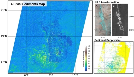
Figure 7 shows the distribution of detected alluvial fine material using the approach presented in Section 4.2.1. The product represents the estimated supply of fresh alluvial sediments for dust emission that is held by each 40 m × 40 m pixel. Three subsets (a, b, c) are presented as zoom-in and compared to Blue Marble true color subsets of the same region to show the AFM in more detail. On these subsets, it is illustrated how the sediment availability lines up with the present river valleys. Subset (a) shows a large wadi running along the mountain range from south to north. This wadi is very well visible on the true color satellite image and holds large amounts of fresh alluvial sediments. Subset (b) covers the southwestern drainage basins with fresh and ancient fluvial systems and thick layers of alluvial sediments. Subset (c) in the center of the mountain range shows wadis with sediments of a different mineralogy indicated by the darker color in the true color image; these wadis are partly covered by vegetation. These qualitative comparisons show that the resulting AFM map is satisfyingly representing the main ephemeral river basins all around the study area. Unfortunately, due to the inaccessibility of the area, reference data of the land surface is very limited, which does not allow for a more quantitative accuracy assessment of the AFM map. However, the results are in alignment with geomorphological studies of the area [34,35], which describe the southwest of the Aïr Massif as the drainage of the mountain range.
The detected ephemeral river basins reach out far from the mountain range and cover the full hot-spot Zone SW. This is indicative of a regular recharge of the alluvial sources in this region. Zone S is influenced by similar river valleys at its northwestern side, however they do not reach out as far into the zone and only cover parts of Zone S. In Zone C, the number of detected active ephemeral streams is much lower, but there is a very large wadi together with some alluvial fans found along the mountain range at the eastern side of Zone C. Besides some narrow wadis, alluvial fine material is not very abundant in Zone N. This can be explained by the higher latitude of the zone, leading to a lower influence of the WAM and consequently to a lower annual precipitation, less surface runoff and very infrequent activation of ephemeral streams.
Besides alluvial fine material, dunes and sand sheets are a second source type which is considered in this study. Figure 4A shows the final SSM map, including the location of detected sand cover together with the categorized alluvial fine material information. The main distribution of sand is found east of the mountain range, where the erg of Bilma, one of the largest sand seas in the Sahara is located [69]. West of the mountain range, however, sand cover is sparsely found.
The SSM was resampled to the model grid of 0.1 × 0.1. The resampled sediment supply map is depicted in Figure 4B.
6.3. Model Simulations of Dust Emission
The DSAF shows a spatiotemporally variable pattern of dust activity throughout the study area. The model study intended to show whether this pattern can be replicated by the dust-emission model. Of particular interest was the benefit of the SSM for the modeling results. Thus, the model was run twice: one run included the SSM information and the size distribution of erodible elements referred to as SSM-run. Additionally, a control run was performed that does not include the SSM but a constant surface type of regs/hamadas throughout the whole study area. The model was driven using the ECMWF external wind field in 10 m height and simulated the dust emission flux in kg/m2/s of the surface for the four-year period 2013–2016 for a 0.1 × 0.1 grid and a temporal resolution of 1 h. The mean annual emission flux in kg/m2 for the SSM run is represented in Figure 8 (left), the control run is depicted in Figure 8 (right). The SSM-run shows increased dust activity for the area southeast to southwest of the mountain range mainly within the bounds of Zones S and SW. Further increased activity is simulated for the eastern part of Zone C and in the region of the sand sea east of the mountain range. In comparison to this, the emission flux of the control run is much smaller throughout the whole study area with relative peaks south and north of the mountain range.
6.3.1. Influence of SSM on Simulated Dust Emission
The spatial distribution of dust activity derived from the model simulations appears to be strongly connected to the SSM (Figure 4), leading to some similarities in the pattern of dust sources and dust activity. This shows how sensitive the model is to the information on soil size distribution. The connection becomes particularly obvious when comparing the SSM run to the control run, where the emission flux was much lower throughout most parts of the study area, indicating a limited sediment supply for these surface assumptions.
To quantify the influence of the SSM on the model results, the mean total annual mass of emission derived from the SSM run for each surface type was compared to the respective pixels of the control run (indicated by the grey shading of the bars), as depicted in Figure 9A. Surfaces identified as medium emitting alluvials are by far the most emitting surfaces with more than 40 kg dust emitted per year throughout the whole study area. This is followed by dunes/sand sheets with 17 kg and alluvial high emitting surfaces with around 10 kg. Compared to the control run, this is a drastic increase of dust emission due to the implementation of the SSM.
Figure 9B depicts the mean emission flux in grams per square metre per year for each source type and hence represents the activity normalized by the area covered by each source type. This shows how active the alluvial high emitting surfaces are compared to the other source types with almost 120 g per square meter and year. This demonstrates how sensitive the model is to the assignment of the correct source information and the determination of soil parameters to the sources. It is difficult to determine whether the configuration used here is appropriate, mainly because direct measurements are not available. However, the DSAF observed from the Desert-Dust-RGB images can help to estimate if the location and the activity of dust sources is determined in an accurate and realistic way.
6.3.2. Comparison DSAF and Model
The spatial distribution of dust activity from satellite observation (Figure 5) and model (Figure 8) shows that both agree in the localization of the dust hot-spots: the southwest and south of the study area has most dust events in the observational result and the highest dust fluxes in the model. Additionally, in the western part of Zone C, where the large wadi systems are located, high dust activity for both the model and the observation can be found. For a better comparison of model and observations on the temporal scale, the modeled continuous emission flux was translated into a discrete number of dust events for each pixel by applying a threshold of 1 × 10⁻⁵ kg/m2. This value was chosen on the basis of Tegen et al. [70], who used a similar threshold of 6 × 10⁻⁵ kg/m2 to compare modeled and observed dust events. The threshold takes into account that very small and/or very short events might not be detectable on the Desert-Dust-RGB product due to its temporal and spatial resolution. Whenever the surface emission flux exceeds the threshold, the modeled emissions were counted as a dust event. In a second step, the total number of dust events was translated into the entity days with dust emission and the monthly mean activity of the model result was calculated and compared to the observational result represented in Figure 6.
Figure 10 (left) shows this monthly mean activity for the four hot-spot zones derived from the SSM-run. In comparison to the observational annual cycle, the seasonality of the four zones is reproduced quite satisfactorily by the model: in Zones N and S, dust emission tends to peak during winter months while the emissions from Zones SW and C peak during July and August. In contrast to this, Figure 10 (right) shows the temporal distribution of dust activity for the control run without sediment supply information. For Zones SW and C, the control run does not show any seasonality; dust activity remains very low throughout the whole year.
While the annual pattern of activity is similar for observation and model, it has to be stated that the model simulated a much higher activity with a factor of 10 compared to the observations.
7. Discussion
7.1. Overestimation of Sediment Supply
The creation of the alluvial fines map and the dune/sand sheets map, and their integration into a sediment supply map, represents an approach allowing for the detection of two important dust source types that are present in the study area. The AFM was derived from the integration of both flow accumulation data based on a digital elevation model and spectral information of the polar-orbiting Sentinel-2 satellite. This integrated two independent levels of information as base for the AFM. Compared to other approaches (e.g., [26,71]), the method presented here uses both the visible and infrared light information, and integrates both into one information band during the HLS-transformation. While the HydroSHEDS flow accumulation is a static dataset, the Sentinel-2 data covers the full globe every five days. Hence, it is possible to use the presented approach for time-variant surfaces, and, due to the global coverage of both datasets, it can be applied for similar studies in all deserts of the globe. However, it needs to be stated that the accuracy of the SSM map is difficult to estimate due to the limitation in adequate ground truth data in quality and quantity. This is why only a short qualitative comparison to other satellite-based replicates (i.e., Google Earth and Blue Marble) of the land surface was performed to assess the quality of the AFM. Nevertheless, the qualitative approach reveals a quite satisfactory performance in the detection of ephemeral river basins in the study area, leading to an accurate detection of the drainage systems found in the southwest of the Aïr Massif. The dune and sand sheets detection approach localizes the main sand seas east of the mountain range, where the great erg of Bilma is located. This shows the ability of this rather simple approach to localize great sand seas. However, the approach is merely based on the brightness of the surface in the visible light, which leads to the inclusion of other bright surfaces into the DSM. This commission error needs to be considered and is likely to lead to an overly high assumption of sediment supply in the model. The integration of the sediment supply information into the model and the accompanied resampling of the original resolution to the model grid is a crucial step in setting up the dust-emission model. The model resolution by far exceeds the size of the identified dust sources, which makes it difficult to bring these features to model resolution without loss of information. We used a strict approach that favors high emitting sources over other surfaces. This possibly leads to a further overestimation of sediment supply in the model. The same is true for the estimation of Z0, for which the SSM map is used. Too generously identified source distribution leads to too low Z0 values.
These are important factors that are able to highly influence the subsequent model results. Nonetheless, the detection of sediment supply in the study area and the integration of this information in the model is an important step towards a better representation of small-scale features and highly improves the model results compared to the control run, which does not include source information.
7.2. Overestimation of Simulated Emission Flux
The simulated dust fluxes show how the model benefits from the integration of sediment supply information: the location of dust hot spots is more accurate, especially for the ephemeral river systems located in Zone SW and for the wadis found along the mountain range in Zone C. These features do not show much dust activity in the control run. By including the SSM, a similar spatial pattern of dust hot-spots compared to the observation could be achieved. The course of the monthly activity and hence the annual variability of dust events for the four zones shows a number of similarities to the observation with a peaking number of dust events in winter during Harmattan period for the Zones S and N and a peak in activity in summer during the WAM phase for the Zones SW and C. However, the simulated dust activity transformed into number of days with dust activity reveals that the model produces around ten times higher activity than the observations. In the following, explanations for this difference between model and observations are given.
(1) The underestimation of the number of dust events that are detected from the observational data: the Desert-Dust-RGB product is dependent on atmospheric parameters such as temperature, relative humidity, clouds, dust layer height, surface emissivity and the aerosol optical thickness of the plume [38,39,70]. These parameters influence how intense the pink color of a dust plume appears on the RGB product and thereby how easy a dust plume is detectable by eye. Missing less distinct dust plumes in the analysis leads to an underestimation of the total number of dust plumes. The same applies for events from sources that are fully covered by clouds and events downwind of an existing dust plume. The temporal and spatial resolution of the Desert-Dust-RGB images further leads to the omission of very short or very small events. All of these factors lead to a tendency to underestimate the number of events. Another disadvantage of the back-tracking method is the limited quantitative information on the thickness of the observed dust plumes, which makes it difficult to compare the discrete number of events from the observation to the continuous dust emission flux simulated by the model. Despite all this, the back-tracking method of the Desert-Dust-RGB product gives the unique opportunity to determine the true source of dust plumes in an accurate way, especially in contrast to products derived from polar-orbiting satellites [13].
(2) The overestimation of the emission flux by the model: besides a possible overestimation of sediment supply discussed above, another reason for an overestimation of the dust flux by the model can be found in the interpretation of the results: the model does not include any information on the transport and deposition of eroded particles. Not every dust emission flux at the surface leads to the dispersion of a real dust plume in the atmosphere. It is conceivable that many particles, although suspended from the surface, are deposited in the direct vicinity of a source. Further, very short or small events do not lead to a dust plume that is detectable by the satellite. Although a threshold was applied on the modeled emission flux to account for these overestimations by the model, the activity of model grid cells is still too high and dust emission begins at wind shear stress values that are too low.
In fact, different threshold values were applied in the interpretation phase of the model result. The value that was finally chosen is in conjunction with the threshold used by Tegen et al. [70]. However, Tegen et al. [70] used a coarser resolution model, which, according to Ridley et al. [72], leads to a lower emission flux due to generalization of the wind field. Hence, the threshold chosen here might be not suitable for the model grid spacing of our study. However, a higher threshold applied on the simulated emission fluxes leads to a main loss in events for the hot-spot Zones SW and C during WAM phase, which lowered the seasonality in the monthly distribution of events in these two zones. This is why, at the expense of keeping the seasonality of dust activity, an overly large activity was accepted.
The less pronounced seasonality when applying a higher threshold, especially in the monsoon-influenced zones, can be explained by the meteorological information that is used to drive the model: while ECMWF ERA-interim data have been frequently used in similar studies [29,59,73], we employed wind velocities obtained from the ECMWF forecast model. This dataset has some limits in predicting convection within the WAM. However, it has one major advantage compared to ERA-Interim data, which is its higher spatial and temporal resolution. To better estimate the influence of the SSM and the small-scale dust sources, high resolution was of great importance for this study and the shortcomings of the dataset were accepted. However, the underestimation of the number of MCS and the lower accuracy in their location lead to fewer days on which the threshold of wind shear stress for dust emission is exceeded. This leads to fewer dust events during the monsoon period, especially in those hot-spot zones that are strongly affected by the MCS.
8. Conclusions
This study represents an extensive analysis of the dust activity for a study area in Niger. The region has been identified as an important dust source in previous studies and was examined in detail in this study. For this, the dust activity was determined for a four-year period and four dust hot-spots were identified. The four hot-spot zones are marked by a distinct seasonality in their dust activity: while, for two of them, the number of dust events peaks during winter, the other two tend to peak during boreal summer. These patterns are based on the location of the hot-spots in respect to the main meteorological features of the area. To determine the geomorphological features that provide the hot-spot regions with erodible particles, an approach was developed that uses the HydroSHEDS flow accumulation data, based on the SRTM digital elevation model, and an HLS transformed false color image of visible and near infrared optical Sentinel-2 data. With this, alluvial fine material found in ephemeral river basins and playas was localized. As an asset, the distribution of a second source type, i.e., sand dunes and sand sheets, was determined based on the brightness of the land surface. The alluvial fine material together with the distribution of sand cover gave information on the sediment supply of the study area. The determined source distribution reveals that the observed dust activity can often be directly connected to the identified sources.
The sediment supply information was implemented in a dust emission model. The results of the dust emission modeling show the benefits of implementing the sediment supply information: the simulated emission flux shows an enhanced representation of the observed dust activity in both spatial distribution of dust sources and temporal variability in the activity of the four hot-spot zones. However, it needs to be stated that the model shows a relative overestimation of dust events compared to the observations. Nevertheless, the model results clearly show how important an accurate source description is to successfully simulating dust emission from small-scale sources. The datasets used for the source identification are available globally. Hence, this approach can be applied in other regional, continental or even global modeling studies. Due to the temporally high coverage of Sentinel-2 scenes and other similar satellites, the approach can also be applied on studies focussing on temporally variable sources.
Author Contributions
Conceptualization, S.F. and K.S.; Data curation, S.F.; Formal analysis, S.F.; Funding acquisition, K.S.; Investigation, S.F.; Methodology, S.F.; Project administration, K.S.; Resources, K.S.; Software, S.F.; Supervision, K.S.; Validation, S.F. and K.S.; Visualization, S.F.; Writing—original draft, S.F.; and Writing—review and editing, S.F. and K.S.
Funding
This research was funded by the Leibniz Association through the project “Dust at the interface—modelling and remote sensing”.
Acknowledgments
The authors acknowledge the providers of the numerous datasets used in this study: NASAs Goddard Earth Science (GES) Data and Information Service Center (DISC) for the provision of the MODIS MYD13A3 product; the ArcGIS REST Service Directory (http://server.arcgisonline.com/arcgis/rest/services) for providing true color imagery of the land surface including NASA’s Blue Marble imagery offered by NASA’s Space Observatory; EUMETSAT for the compilation and provision of the Desert-Dust-RGB imagery; the European Space Agency (ESA) for providing free-of-charge Sentinel-2 data and Copernicus for making these data accessible through its scientific hub (https://scihub.copernicus.eu/); the providers of the HydroSHEDS dataset freely available at http://www.hydrosheds.org; and ECMWF for the provision of high resolution forecast data (http://apps.ecmwf.int/datasets/).
Conflicts of Interest
The authors declare no conflict of interest. The funders had no role in the design of the study; in the collection, analyses, or interpretation of data; in the writing of the manuscript, or in the decision to publish the results.
References
- Ginoux, P.; Prospero, J.M.; Gill, T.E.; Hsu, N.C.; Zhao, M. Global-scale attribution of anthropogenic and natural dust sources and their emission rates based on MODIS Deep Blue aerosol products. Rev. Geophys. 2012, 50. [Google Scholar] [CrossRef] [Green Version]
- Washington, R.; Bouet, C.; Cautenet, G.; Mackenzie, E.; Ashpole, I.; Engelstaedter, S.; Lizcano, G.; Henderson, G.; Schepanski, K.; Tegen, I. Dust as a tipping element: The Bodélé Depression, Chad. Proc. Natl. Acad. Sci. USA 2009, 106, 20564–20571. [Google Scholar] [CrossRef] [PubMed]
- Washington, R.; Todd, M.C.; Lizcano, G.; Tegen, I.; Flamant, C.; Koren, I.; Ginoux, P.; Engelstaedter, S.; Bristow, C.S.; Zender, C.S.; et al. Links between topography, wind, deflation, lakes and dust: The case of the Bodélé Depression, Chad. Geophys. Res. Lett. 2006, 33. [Google Scholar] [CrossRef] [Green Version]
- Todd, M.C.; Washington, R.; Martins, J.V.; Dubovik, O.; Lizcano, G.; M’Bainayel, S.; Engelstaedter, S. Mineral dust emission from the Bodélé Depression, northern Chad, during BoDEx 2005. J. Geophys. Res. 2007, 112. [Google Scholar] [CrossRef] [Green Version]
- Schepanski, K.; Tegen, I.; Todd, M.C.; Heinold, B.; Bönisch, G.; Laurent, B.; Macke, A. Meteorological processes forcing Saharan dust emission inferred from MSG-SEVIRI observations of subdaily dust source activation and numerical models. J. Geophys. Res. 2009, 114. [Google Scholar] [CrossRef] [Green Version]
- Wagner, R.; Schepanski, K.; Heinold, B.; Tegen, I. Interannual variability in the Saharan dust source activation- Toward understanding the differences between 2007 and 2008. J. Geophys. Res. Atmos. 2016, 121, 4538–4562. [Google Scholar] [CrossRef]
- Prospero, J.M.; Ginoux, P.; Torres, O.; Nicholson, S.E.; Gill, T.E. Environmental characteristics of global sources of atmospheric soil dust identified with the Nimbus 7 Total Ozone Mapping Spectrometer (TOMS) Absorbing Aerosol Product. Rev. Geophys. 2002, 40. [Google Scholar] [CrossRef]
- Herman, J.; Bhartia, P.; Torres, O.; Hsu, C.; Seftor, C.; Celarier, E. Global distribution of UV-absorbing Aerosols from Nimbus 7/TOMS data. J. Geophys. Res. Atmos. 1997, 102, 16911–16922. [Google Scholar] [CrossRef]
- Washington, R.; Todd, M.; Middleton, N.J.; Goudie, A.S. Dust-Storm Source Areas Determined by the Total Ozone Monitoring Spectrometer and Surface Observations. Ann. Assoc. Am. Geogr. 2003, 93, 297–313. [Google Scholar] [CrossRef]
- Ginoux, P.; Garbuzov, D.; Hsu, N.C. Identification of anthropogenic and natural dust sources using Moderate Resolution Imaging Spectroradiometer (MODIS) Deep Blue level 2 data. J. Geophys. Res. 2010, 115. [Google Scholar] [CrossRef] [Green Version]
- Schepanski, K.; Tegen, I.; Laurent, B.; Heinold, B.; Macke, A. A new Saharan dust source activation frequency map derived from MSG-SEVIRI IR-channels. Geophys. Res. Lett. 2007, 34. [Google Scholar] [CrossRef] [Green Version]
- Baddock, M.; Bullard, J.; Bryant, R. Dust source identification using MODIS: A comparison technique applied to the Lake Eyre Basin, Australia. Remote Sens. Environ. 2009, 113, 1511–1528. [Google Scholar] [CrossRef]
- Schepanski, K.; Tegen, I.; Macke, A. Comparison of satellite based observations of Saharan dust source areas. Remote Sens. Environ. 2012, 123, 90–97. [Google Scholar] [CrossRef]
- Reheis, M.; Kihl, R. Dust deposition in southern Nevada and California, 1984–1989: Relations to climate, source area, and source lithology. J. Geophys. Res. 1995, 100, 8893–8918. [Google Scholar] [CrossRef]
- Ryder, C.L.; Highwood, E.J.; Lai, T.M.; Sodemann, H.; Marsham, J.H. Impact of atmospheric transport on the evolution of microphysical and optical properties of Saharan dust. Geophys. Res. Lett. 2013, 40, 2433–2438. [Google Scholar] [CrossRef] [Green Version]
- Schepanski, K.; Flamant, C.; Chaboureau, J.P.; Kocha, C.; Banks, J.R.; Brindley, H.E.; Lavaysse, C.; Marnas, F.; Pelon, J.; Tulet, P. Characterization of dust emission from alluvial sources using aircraft observations and high-resolution modeling. J. Geophys. Res. Atmos. 2013, 118, 7237–7259. [Google Scholar] [CrossRef] [Green Version]
- Baddock, M.; Ginoux, P.; Bullard, J.; Gill, T. Do MODIS defined dust sources have a geomorphological signature? Geophys. Res. Lett. 2016, 43, 2606–2613. [Google Scholar] [CrossRef]
- Lee, J.; Baddock, M.; Mbuh, M.; Gill, T. Geomorphic and land cover characteristics of aeolian dust sources in West Texas and eastern New Mexico, USA. Aeolian Res. 2011, 3, 459–466. [Google Scholar] [CrossRef]
- von Holdt, J.; Eckardt, F.; Wiggs, G. Landsat identifies dust emission dynamics at the landform scale. Remote Sens. Environ. 2017, 198, 229–243. [Google Scholar] [CrossRef]
- Bryant, R. Recent advances in our understanding of dust source emission processes. Prog. Phys. Geogr. 2013, 37, 397–421. [Google Scholar] [CrossRef]
- Vickery, K.; Eckardt, F.; Bryant, R. A sub-basin scale dust plume source frequency inventory for southern Africa, 2005–2008. Geophys. Res. Lett. 2013, 40, 5274–5279. [Google Scholar] [CrossRef]
- Bullard, J.; Harrison, S.P.; Baddock, M.C.; Drake, N.; Gill, T.E.; McTainsh, G.; Sun, Y. Preferential dust sources: A geomorphological classification designed for use in global dust-cycle models. J. Geophys. Res. 2011, 116, F04034. [Google Scholar] [CrossRef]
- Parajuli, S.; Yang, Z.L.; Kocurek, G. Mapping erodibility in dust source regions based on geomorphology, meteorology, and remote sensing. J. Geophys. Res. Earth Surf. 2014, 119, 1977–1994. [Google Scholar] [CrossRef] [Green Version]
- Huneeus, N.; Schulz, M.; Balkanski, Y.; Griesfeller, J.; Kinne, S.; Prospero, J.; Bauer, S.; Boucher, O.; Chin, M.; Dentener, F.; et al. Global dust model intercomparison in AeroCom phase I. Atmos. Chem. Phys. 2011, 11. [Google Scholar] [CrossRef]
- Evan, A.; Flamant, C.; Fiedler, S.; Doherty, O. An analysis of aeolian dust in climate models. Geophys. Res. Lett. 2014, 41, 5996–6001. [Google Scholar] [CrossRef] [Green Version]
- Parajuli, S.P.; Zender, C.S. Connecting geomorphology to dust emission through high-resolution mapping of global land cover and sediment supply. Aeolian Res. 2017, 27, 47–65. [Google Scholar] [CrossRef]
- Marticorena, B.; Bergametti, G. Modeling the atmospheric dust cycle: 1. Design of a soil-derived dust emission scheme. J. Geophys. Res. 1995, 100, 16–415. [Google Scholar] [CrossRef]
- BouKaram, D.; Flamant, C.; Knippertz, P.; Reitebuch, O.; Pelon, P.; Chong, M.; Dabas, A. Dust emissions over the Sahel associated with the West African Monsoon inter-tropical discontinuity region: A representative case study. Q. J. R. Meteorol. Soc. 2008, 134, 621–634. [Google Scholar] [CrossRef]
- Fiedler, S.; Schepanski, K.; Heinold, B.; Knippertz, P.; Tegen, I. Climatology of nocturnal low-level jets over North Africa and implications for modeling mineral dust emission. J. Geophys. Res. Atmos. 2013, 118, 6100–6121. [Google Scholar] [CrossRef] [Green Version]
- Roberts, A.; Knippertz, P. Haboobs: Convectively generated dust storms in West Africa. Weather 2012, 67, 311–316. [Google Scholar] [CrossRef]
- Heinold, B.; Knippertz, P.; Marsham, J.H.; Fiedler, S.; Dixon, N.S.; Schepanski, K.; Laurent, B.; Tegen, I. The role of deep convection and nocturnal low-level jets for dust emission in summertime West Africa: Estimates from convection-permitting simulations. J. Geophys. Res. Atmos. 2013, 118, 4385–4400. [Google Scholar] [CrossRef] [Green Version]
- Knippertz, P.; Todd, M.C. The central west Saharan dust hot spot and its relation to African easterly waves and extratropical disturbances. J. Geophys. Res. 2010, 115. [Google Scholar] [CrossRef] [Green Version]
- Vanmaercke, M.; Zenebe, A.; Poesen, J.; Nyssen, J.; Verstraeten, G.; Deckers, J. Sediment dynamics and the role of flash floods in sediment export from medium-sized catchments: A case study from the semi-arid tropical highlands in northern Ethiopia. J. Soils Sediments 2010, 10, 611–627. [Google Scholar] [CrossRef]
- Schlüter, T. Geological Atlas of Africa: With Notes on Stratigraphy, Tectonics, Economic Geology, Geohazards and Geosites of each Country; Springer: Berlin, Germany, 2008. [Google Scholar]
- Wright, B. Geology and Mineral Resources of West Africa; Springer: Dordrecht, The Netherlands, 1985. [Google Scholar]
- Graef, F.; Vennemann, K. The Geological Setting in Western Niger. 1999. Available online: https://www.uni-hohenheim.de/atlas308/b_niger/projects/b2_1_1/html/english/nframe_en_b2_1_1.htm (accessed on 23 May 2017).
- Schmetz, J.; Pili, P.; Tjemkes, S.; Just, D.; Kerkmann, J.; Rota, S.; Ratier, A. An introduction to Meteosat Second Generation (MSG). Bull. Am. Meteorol. Soc. 2002, 83, 977–992. [Google Scholar] [CrossRef]
- Banks, J.R.; Brindley, H.E. Evaluation of MSG-SEVIRI mineral dust retrieval products over North Africa and the Middle East. Remote Sens. Environ. 2013, 128, 58–73. [Google Scholar] [CrossRef]
- Banks, J.R.; Schepanski, K.; Heinold, B.; Hünerbein, A.; Brindley, H.E. The influence of dust optical properties on the colour of simulated MSG-SEVIRI Desert Dust infrared imagery. Atmos. Chem. Phys. 2018, 18, 9681–9703. [Google Scholar] [CrossRef]
- Lensky, I.M.; Rosenfeld, D. Clouds-Aerosols-Precipitation Satellite Analysis Tool (CAPSAT). Atmos. Chem. Phys. 2008, 8, 6739–6753. [Google Scholar] [CrossRef] [Green Version]
- Fletcher, K. Sentinel-2: ESA’s Optical High-Resolution Mission for GMES Operational Services; ESA SP-1322; ESA: Hong Kong, China, 2012. [Google Scholar]
- Mueller-Wilm, W. Sen2Cor Configuration and User Manual; Ref. S2-PDGS-MPC-L2A-SUM-V2.3; EESA: Paris, France, 2016. [Google Scholar]
- Kim, D.; Chin, M.; Remer, L.; Diehl, T.; Bian, H.; Yu, H.; Brown, M.; Stockwell, W. Role of surface wind and vegetation cover in multi-decadal variations of dust emission in the Sahara and Sahel. Atmos. Environ. 2002, 148, 282–296. [Google Scholar] [CrossRef]
- Huete, A.; Didan, K.; Miura, T.; Rodriguez, E.; Gao, X.; Ferreira, L. Overview of the radiometric and biophysical performance of the MODIS vegetation indices. Remote Sens. Environ. 2002, 83, 195–213. [Google Scholar] [CrossRef]
- Didan, K. MYD13A3 MODIS/Aqua Vegetation Indices Monthly L3 Global 1 km SIN Grid V006 [Data Set]; NASA EOSDIS LP DAAC: Sioux Falls, SD, USA, 2015; Volume 20, pp. 397–398.
- Fensholt, R.; Rasmussen, K.; Nielsen, T.; Mbow, C. Evaluation of earth observation based long term vegetation trends—Intercomparing NDVI time series trend analysis consistency of Sahel from AVHRR GIMMS, Terra MODIS and SPOT VGT data. Remote Sens. Environ. 2009, 113, 1886–1898. [Google Scholar] [CrossRef]
- Schepanski, K.; Wright, T.J.; Knippertz, P. Evidence for flash floods over deserts from loss of coherence in InSAR imagery. J. Geophys. Res. 2012, 117. [Google Scholar] [CrossRef] [Green Version]
- Crouvi, O.; Schepanski, K.; Amit, R.; Gillespie, A.; Enzel, Y. Multiple dust sources in the Sahara Desert: The importance of sand dunes. Geophys. Res. Lett. 2012, 39. [Google Scholar] [CrossRef] [Green Version]
- Huang, Y.; Kok, J.F.; Martin, R.; Swet, N.; Katra, I.; Gill, T.; Reynolds, R.; Freire, L. Fine dust emissions from active sands at coastal Oceano Dunes. Atmos. Chem. Phys. Discuss. 2018. [Google Scholar] [CrossRef]
- Zender, C.S.; Bian, H.; Newman, D. Mineral Dust Entrainment and Deposition (DEAD) model: Description and 1990s dust climatology. J. Geophys. Res. 2003, 108. [Google Scholar] [CrossRef] [Green Version]
- Lehner, B.; Verdin, K.; Jarvis, A. New global hydrography derived from spaceborne elevation data. Eos Trans. Am. Geophys. Union 2008, 89, 93–94. [Google Scholar] [CrossRef]
- Bastawesy, M.E.; White, K.; Nasr, A. Integration of remote sensing and GIS for modelling flash floods in Wadi Hudain catchment, Egypt. Hydrol. Process. 2009, 23, 1359–1368. [Google Scholar] [CrossRef]
- Ford, A.; Roberts, A. Color Space Conversion. Technical Report. 1998. Available online: http://poynton.ca/PDFs/coloureq.pdf (accessed on 23 May 2017).
- Lancaster, N.; Wolfe, S.; Thomas, D.; Bristow, C.; Bubenzer, O.; Burrough, S.; Duller, G.; Halfen, P.H.A.; Roskin, J.; Singhvi, A.; et al. The INQUA Dune Atlas chronologic database. Q. Int. 2015, 1. [Google Scholar] [CrossRef]
- FAO/IIASA/ISRIC/ISSCAS/JRC. Harmonized World Soil Database (Version 1.2). 2012. Available online: http://www.fao.org/soils-portal/soil-survey/soil-maps-and-databases/harmonized-world-soil-database-v12/en/ (accessed on 23 May 2017).
- Hugenholtz, C.H.; Levin, N.; Barchyn, T.; Baddock, M. Remote sensing and spatial analysis of aeolian sand dunes: A review and outlook. Earth Sci. Rev. 2012, 111. [Google Scholar] [CrossRef]
- Chatenet, B.; Marticorena, B.; Gomes, L.; Bergametti, G. Assessing the microped size distributions of desert soils erodible by wind. Sedimentology 1996, 43, 901–911. [Google Scholar] [CrossRef]
- Marticorena, B.; Bergametti, G.; Aumont, B. Modelling the atmospheric dust cycle: 2. Simulation of Saharan dust sources. J. Geophys. Res. 1997, 102, 4387–4404. [Google Scholar] [CrossRef]
- Laurent, B.; Marticorena, B.; Bergametti, G.; Léon, J.F.; Mahowald, N.M. Modeling mineral dust emissions from the Sahara using new surface properties and soil database. J. Geophys. Res. 2008, 113. [Google Scholar] [CrossRef]
- Menut, L.; Pérez, C.; Haustein, K.; Bessagnet, B.; Prigent, C.; Alfaro, S. Impact of surface roughness and soil texture on mineral dust emission fluxes modeling. J. Geophys. Res. 2013, 118. [Google Scholar] [CrossRef]
- Shao, Y.; Raupach, M.R.; Findlater, P.A. Effect of Saltation Bombardment on the Entrainment of Dust by Wind. J. Geophys. Res. 1993, 98, 12719–12726. [Google Scholar] [CrossRef]
- White, B.R. Soil Transport by Winds on Mars. J. Geophys. Res. 1979, 84, 4643–4651. [Google Scholar] [CrossRef]
- Callot, Y.; Marticorena, B.; Bergametti, G. Geomorphologic approach for modelling the surface features of arid environments in a model of dust emission: Application to the Sahara desert. Geodin. Acta 2000, 13, 245–270. [Google Scholar] [CrossRef]
- Laurent, B.; Marticorena, B.; Bergametti, G.; Chazette, P.; Maignan, F.; Schmechtig, C. Simulation of the mineral dust emission frequencies from desert areas of China and Mongolia using an aerodynamic roughness length map derived from the POLDER/ADEOS 1 surface productse. J. Geophys. Res. 2005, 110. [Google Scholar] [CrossRef]
- Knorr, W.; Heimann, M. Impact of drought stress and other factors on seasonal land biosphere CO2 exchange studied through an atmospheric tracer transport model. Tellus B 1995, 47, 471–489. [Google Scholar] [CrossRef]
- Kaplan, J.; Bigelow, N.; Prentice, I.; Harrison, S.; Bartlein, P.J.; Cramer, W.; Marveyeva, N.; McGuire, A.; Murray, D.; Razzhivin, V.; et al. Climate change and Arctic ecosystems: 2. Modeling, paleodata-model comparison and future projections. J. Geophys. Res. 2003, 108, 8171. [Google Scholar] [CrossRef]
- Stockli, R.; Vermote, E.; Saleous, N.; Simmon, R.; Herring, D. The Blue Marble Next Generation—A True Color Earth Dataset Including Seasonal Dynamics from MODIS; NASA Earth Observatory: Washington, DC, USA, 2005.
- Cohen-Zada, A.; Maman, S.; Blumberg, D. Earth aeolian wind streaks: Comparison to wind data from model and stations. J. Geophys. Res. Planets 2017, 122, 1119–1137. [Google Scholar] [CrossRef]
- Mainguet, M.; Chemin, M. Sand Seas of the Sahara and Sahel: An Explanation of their Thickness ans Sand Dune Type by the Sand Budget Principle. Dev. Sedimentol. 1983, 38, 353–363. [Google Scholar] [CrossRef]
- Tegen, I.; Schepanski, K.; Heinold, B. Comparing two years of Saharan dust source activation obtained by regional modelling and satellite observations. Atmos. Chem. Phys. 2013, 13, 2381–2390. [Google Scholar] [CrossRef] [Green Version]
- Grini, A.; Myhre, G.; Zender, C.S.; Isaksen, I.S.A. Model simulation of dust sources and transport in the global atmosphere. Effects of soil erodibility and wind speed variability. J. Geophys. Res. 2005, 110. [Google Scholar] [CrossRef]
- Ridley, D.; Heald, C.; Pierce, J.; Evans, M. Toward resolution-independent dust emissions in global models: Impacts on the seasonal and spatial distribution of dust. Geophys. Res. Lett. 2013, 40, 2873–2877. [Google Scholar] [CrossRef] [Green Version]
- Tegen, I.; Harrison, S.P.; Kohfeld, K.; Prentice, I.C.; Coe, M.; Heimann, M. Impact of vegetation and preferential source areas on global dust aerosol: Results from a model study. J. Geophys. Res. 2002, 107. [Google Scholar] [CrossRef]
Figure 1.
Overview of the location of the study area, the Bodélé depression, and the main Saharan mountain ranges, as well as the location of the West African Monsoon and Harmattan winds.
Figure 1.
Overview of the location of the study area, the Bodélé depression, and the main Saharan mountain ranges, as well as the location of the West African Monsoon and Harmattan winds.

Figure 2.
(A) Extraction of Alluvial Fines Map (AFM) from HydroSHEDS flow accumulation dataset and Sentinel-2 bands B12, B7, and B4; and (B) derivation of Dune/Sand Cover Map (DSM) from Sentinel-2 bands B4, B3 and B2 and their integration into a Sediment Supply Map (SSM).
Figure 2.
(A) Extraction of Alluvial Fines Map (AFM) from HydroSHEDS flow accumulation dataset and Sentinel-2 bands B12, B7, and B4; and (B) derivation of Dune/Sand Cover Map (DSM) from Sentinel-2 bands B4, B3 and B2 and their integration into a Sediment Supply Map (SSM).

Figure 3.
Example of a river bed in the study area on: (A) the Sentinel-2 false color RGB image created from bands 12, 7, and 4; and (B) the extracted H-band derived from the HLS transformation of the RGB image.
Figure 3.
Example of a river bed in the study area on: (A) the Sentinel-2 false color RGB image created from bands 12, 7, and 4; and (B) the extracted H-band derived from the HLS transformation of the RGB image.

Figure 4.
Sediment Supply Map (SSM) including dunes and sand sheets (DS), medium emitting alluvial (AM), and high emitting alluvial sediments (AH) for: (A) the original resolution; and (B) after the resampling to model grid spacing; and (C) the aerodynamic roughness length of the overall surface (Z0) adapted as described in Section 5 in model grid spacing.

Figure 5.
Total number of dust events for the Aïr Massif observed on the MSG Desert-Dust-RGB images between 2013 and 2016 and the division of the study area into four dust-hot-spot-zones (A); and true color image of the study area including the hot-spot zones (B).
Figure 5.
Total number of dust events for the Aïr Massif observed on the MSG Desert-Dust-RGB images between 2013 and 2016 and the division of the study area into four dust-hot-spot-zones (A); and true color image of the study area including the hot-spot zones (B).

Figure 6.
Monthly mean dust activity for all grid cells within each of the four hot-spot zones.

Figure 7.
Alluvial Fines Map (AFM) derived from combination of HydroSHEDS FA dataset and the hue transformed band of Sentinel-2 channels 12-7-4. Values close to 1 represent high availability of alluvial sediments. Subsets (a), (b) and (c) show subsets of the AFM map within the study area together with the respective Blue Marble extent.

Figure 8.
Modeled dust source activation frequency for the study area including the four hot spot zones determined in the satellite-based DSAF-analysis (Figure 5) for the original model run including the SSM run (A) and for the control run (B) with constant size distribution of available aggregates.

Figure 9.
Total dust emission flux for each surface type (DS, Dune/Sand sheet; AM, Medium emitting alluvial; AH, High emitting alluvial) and total emission flux derived from control run (grey) for the same cells (A); and spatial mean of total emission flux for each cell and surface type (B).
Figure 9.
Total dust emission flux for each surface type (DS, Dune/Sand sheet; AM, Medium emitting alluvial; AH, High emitting alluvial) and total emission flux derived from control run (grey) for the same cells (A); and spatial mean of total emission flux for each cell and surface type (B).

Figure 10.
Temporal variability of dust activity for the grid cells within each of the hot-spot zones, derived from simulated emission flux of the SSM-run (left) and the control run (right).
Figure 10.
Temporal variability of dust activity for the grid cells within each of the hot-spot zones, derived from simulated emission flux of the SSM-run (left) and the control run (right).


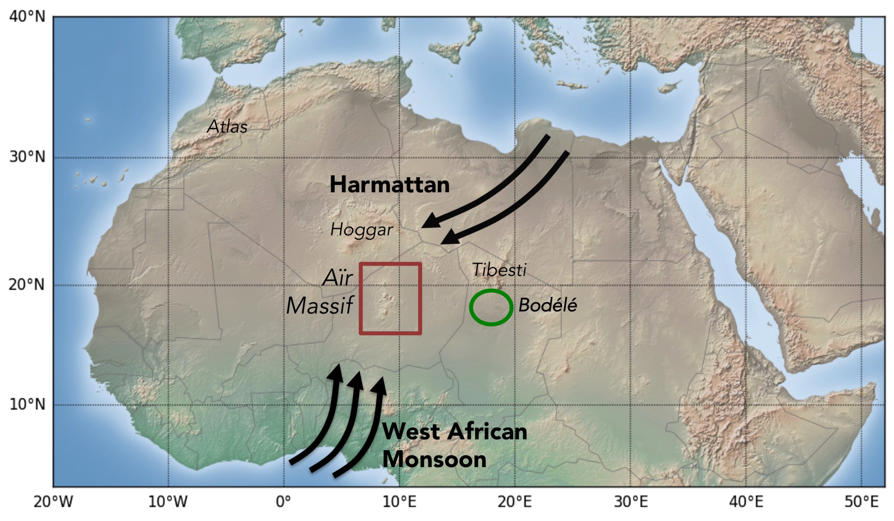
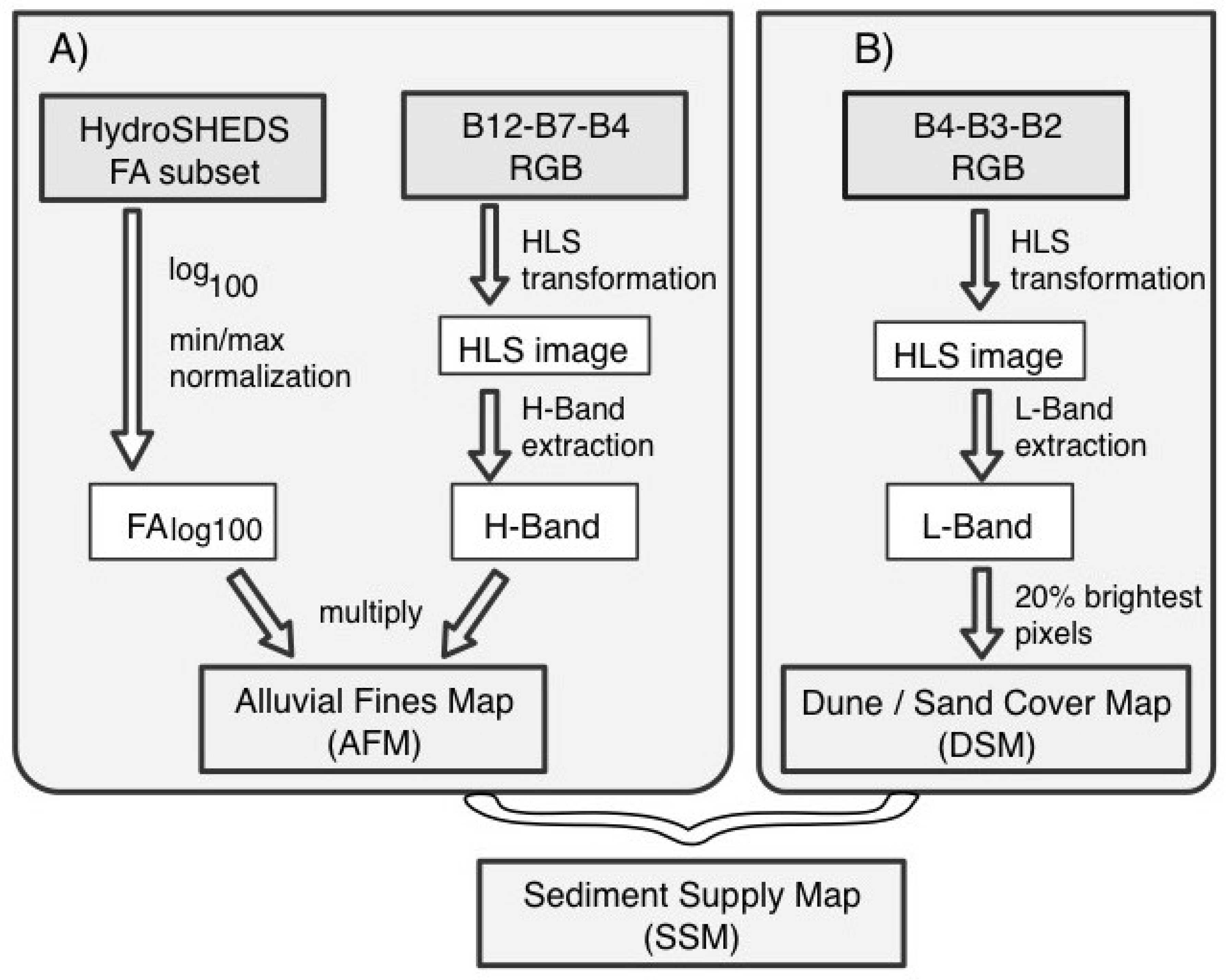
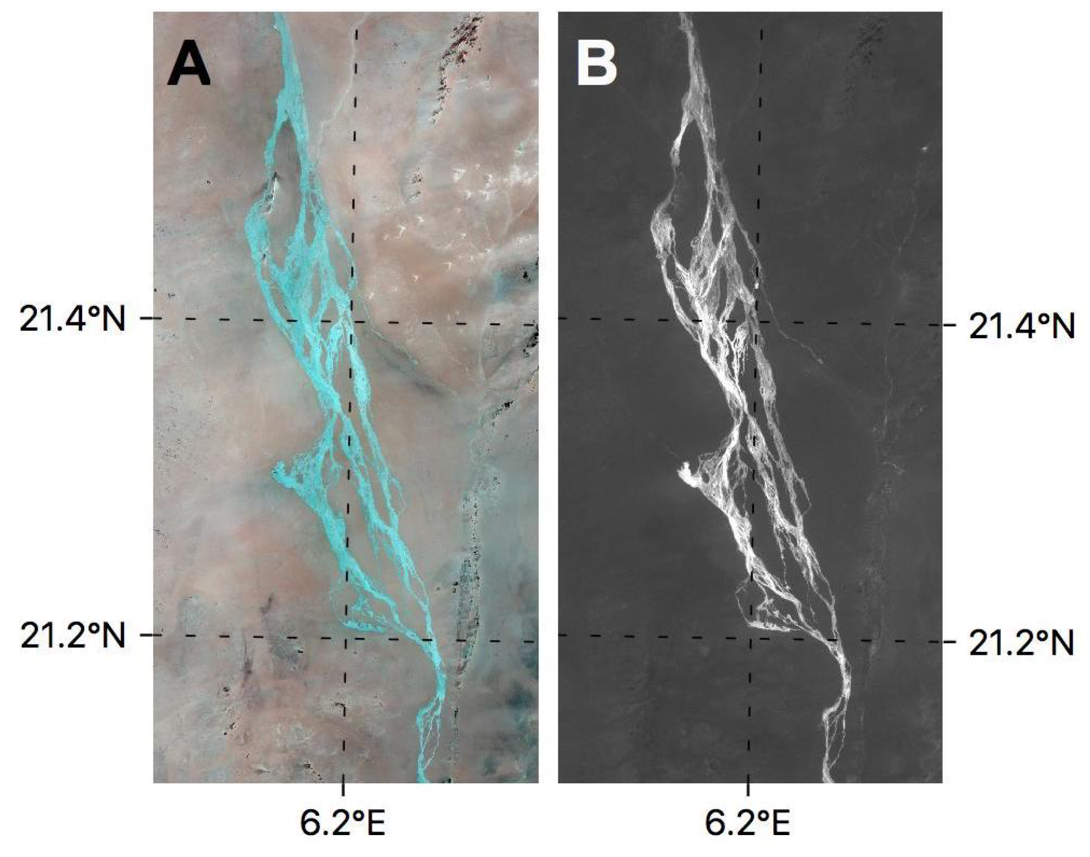
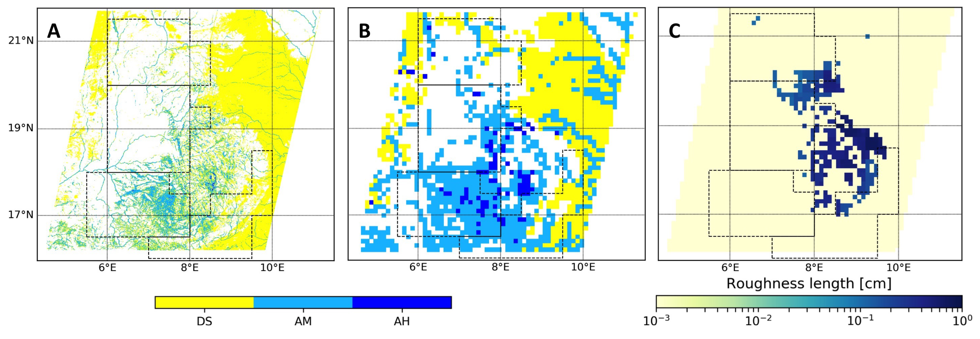
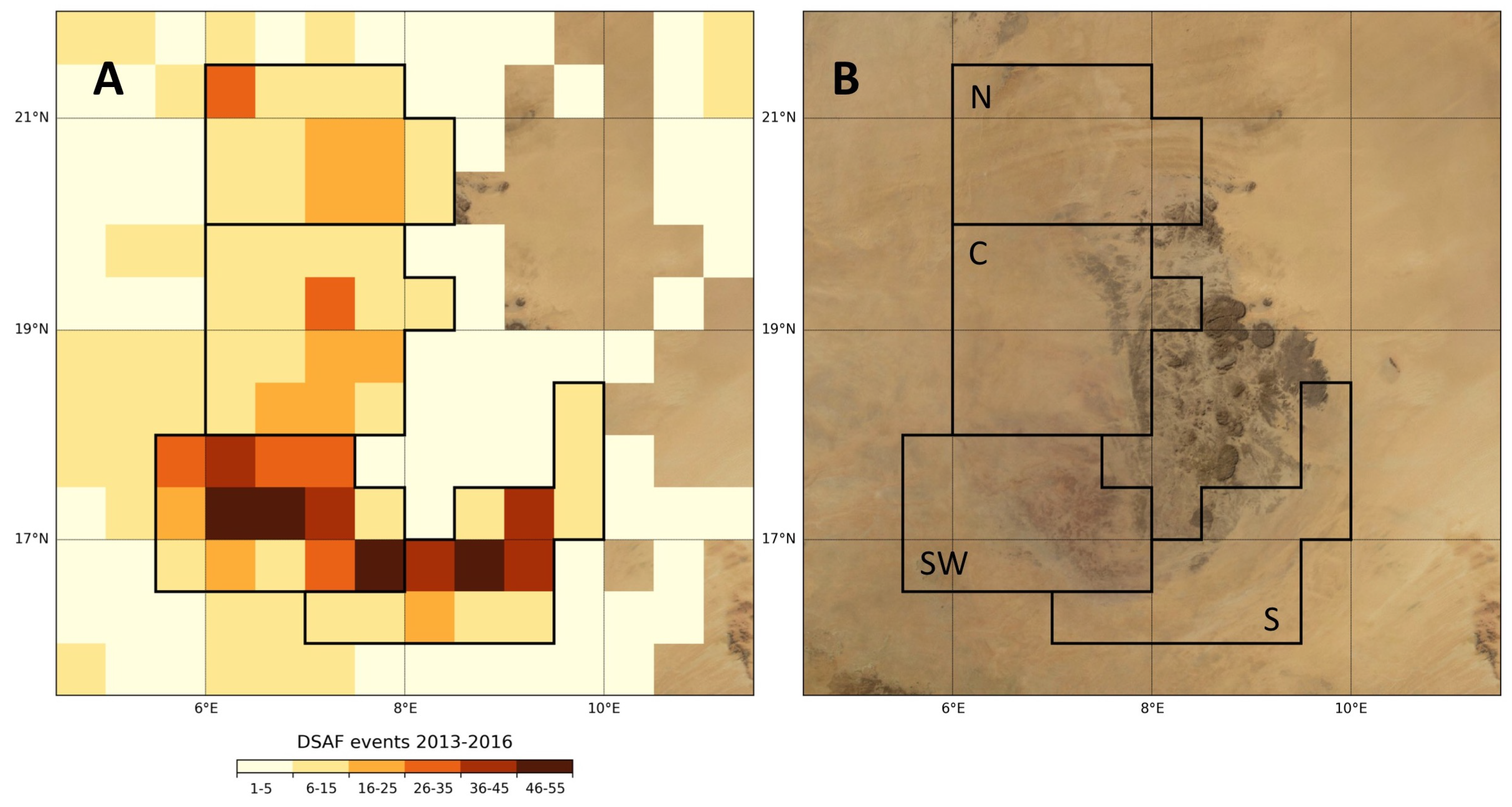
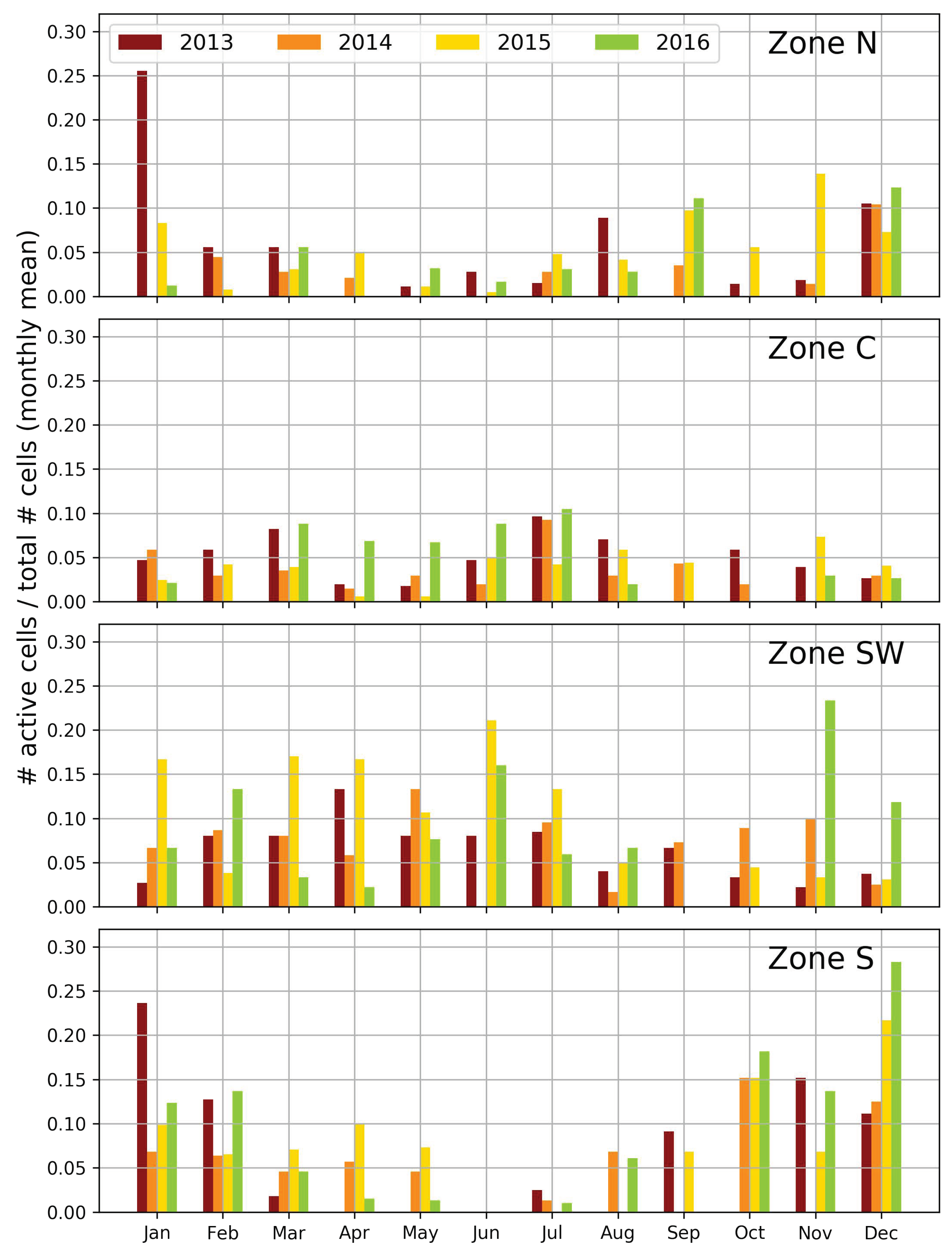
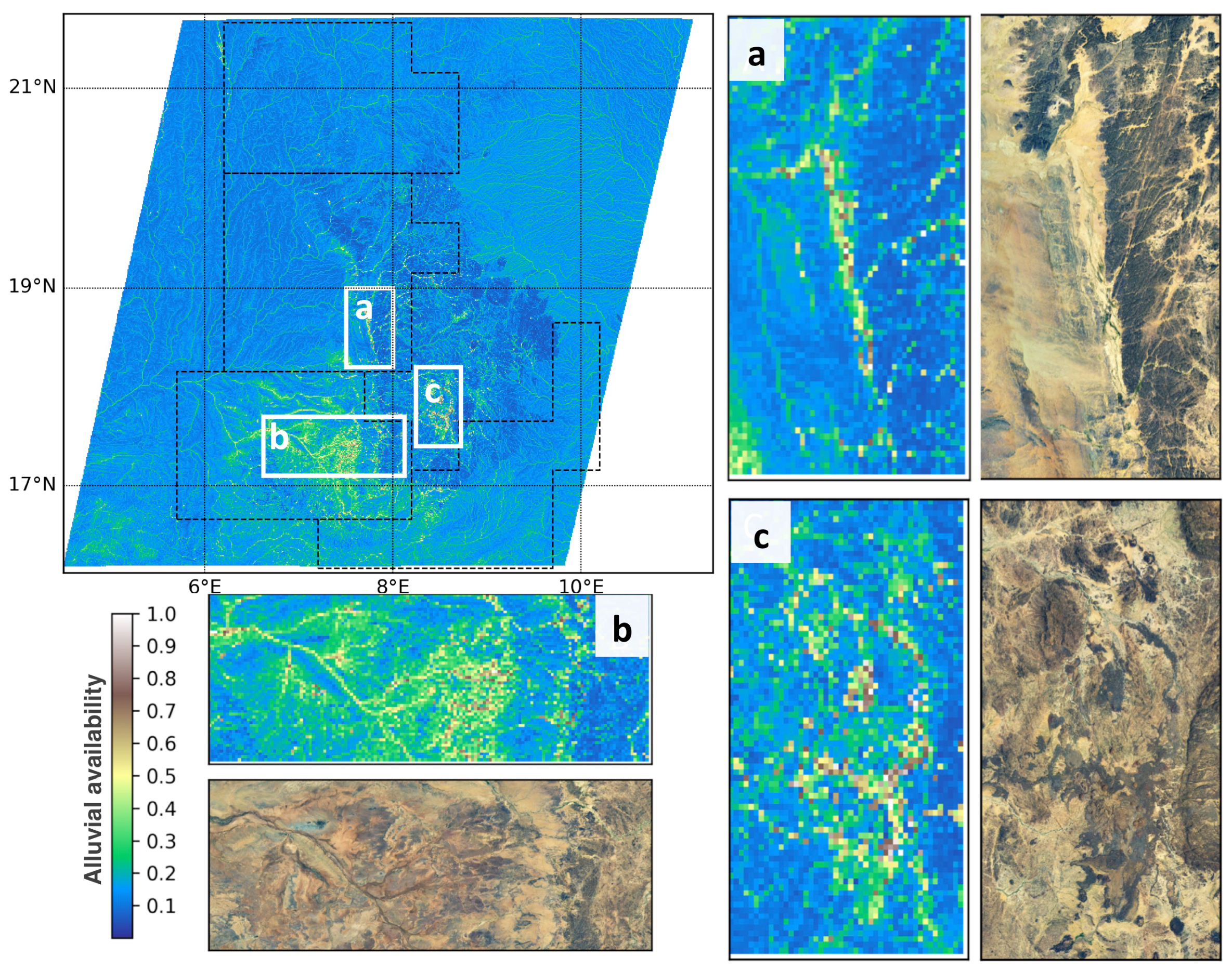
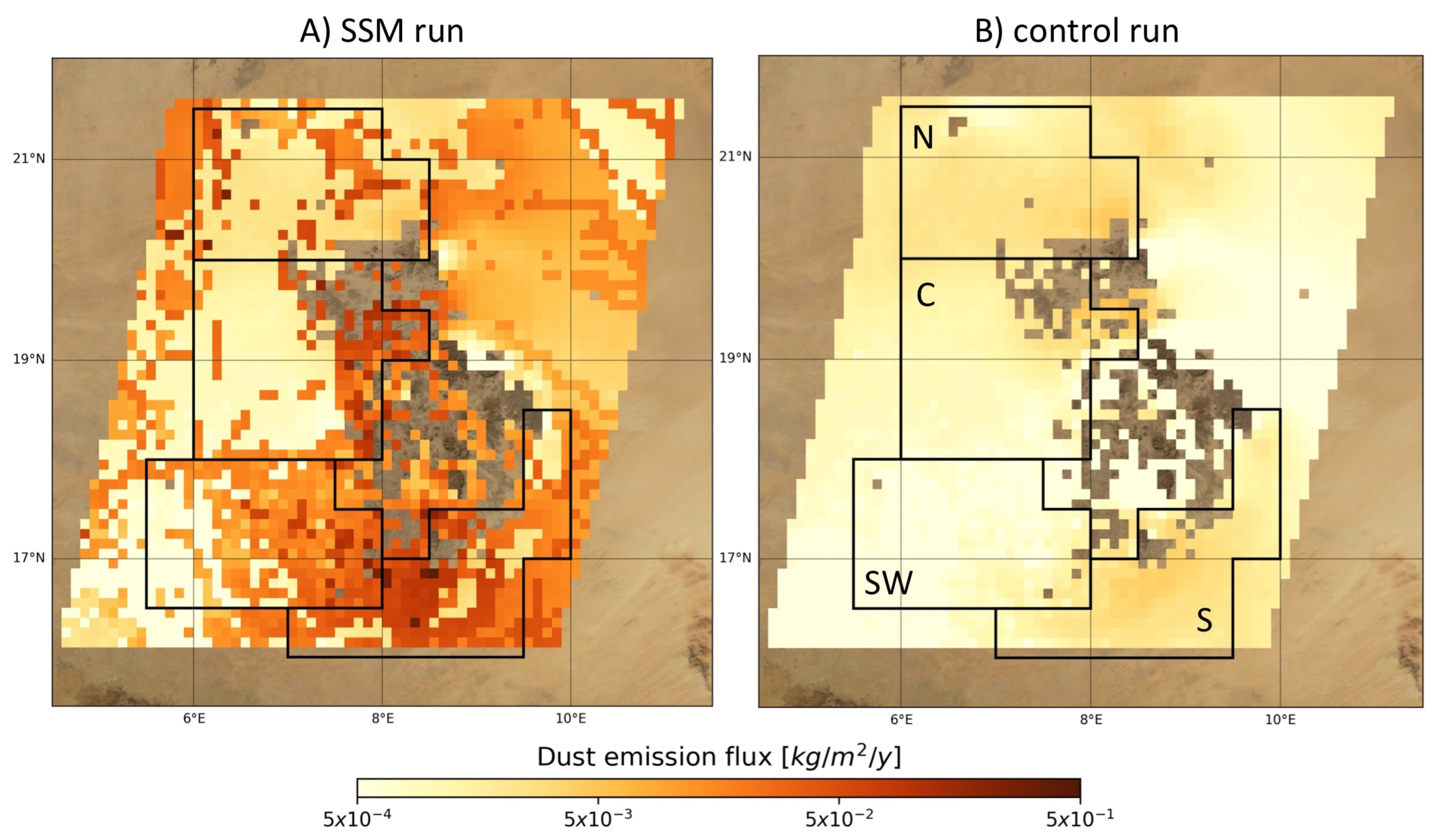
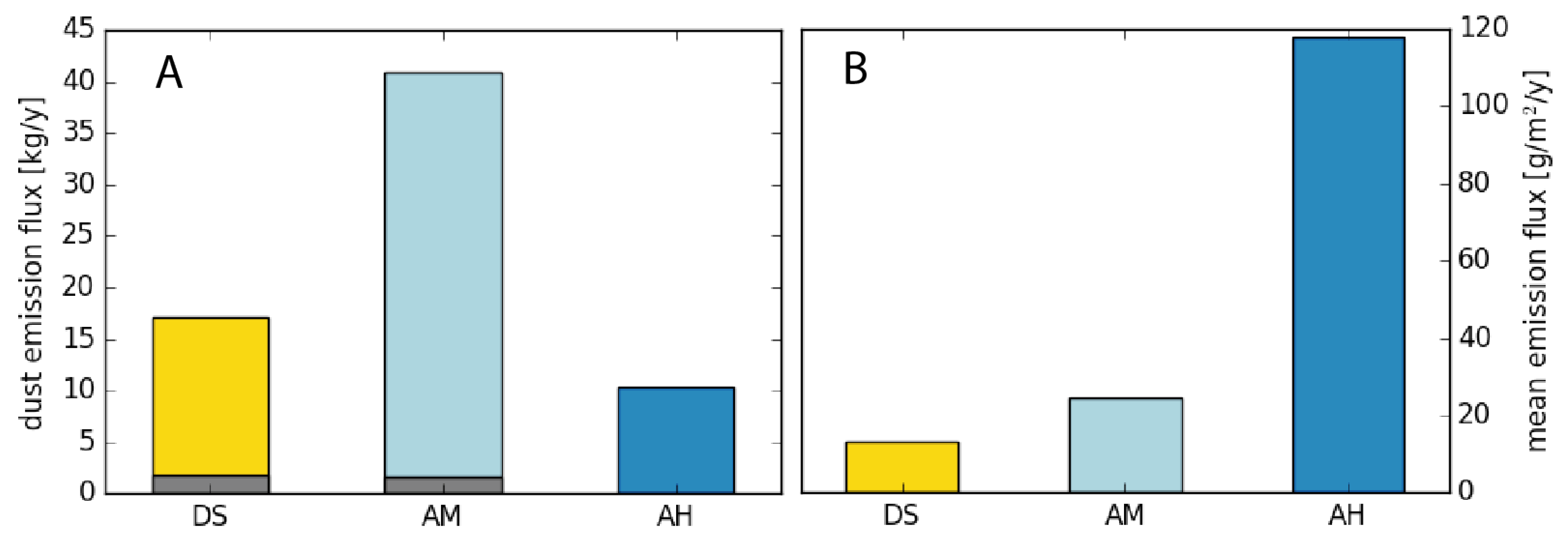
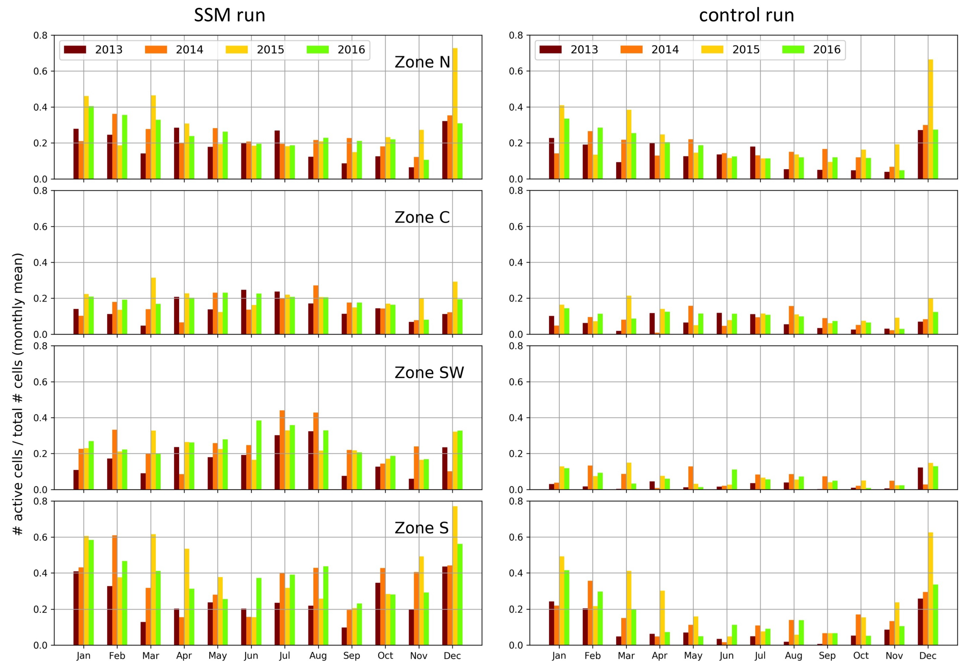
Table 1.
Sensing date and row number of Sentinel-2 images used for the detection of alluvial sediments in the study area.
Table 1.
Sensing date and row number of Sentinel-2 images used for the detection of alluvial sediments in the study area.
| # | Sensing Date | Row Number |
|---|---|---|
| 1 | 3 May 2016 | R079 |
| 2 | 2 June 2016 | R079 |
| 3 | 16 May 2016 | R122 |
| 4 | 5 June 2016 | R122 |
Table 2.
Statistical parameters of the soil size distributions assumed for the present surface types according to Marticorena et al. [58] and Laurent et al. [59] that were used for the model implementation of the SSM. represents the respective saltation efficiency of the surface types, defined by Equation (11).
| Typology | Surface Type | Dmed [] | % | ||
|---|---|---|---|---|---|
| regs/hamadas | CMS | 210 | 1.8 | 10.0 | 1.34 × 10 |
| 690 | 1.6 | 90.0 | |||
| dunes/sand sheets | SMS | 125 | 1.6 | 37.5 | 4.35 × 10 |
| 210 | 1.8 | 31.2 | |||
| 690 | 1.6 | 31.3 | |||
| medium emitting alluvial | SFS | 125 | 1.6 | 37.5 | 6.15 × 10 |
| 210 | 1.8 | 62.5 | |||
| high emitting alluvial | S | 125 | 1.6 | 100 | 1.99 × 10 |
Table 3.
Percentage of clay content of four mineralogical populations determined for desert soils [58].
Table 3.
Percentage of clay content of four mineralogical populations determined for desert soils [58].
| Typology | % Clay |
|---|---|
| alumino-silicated silts | 9.7 |
| fine sand | 3.6 |
| coarse sand | 0 |
| salts | 3.2 |
© 2018 by the authors. Licensee MDPI, Basel, Switzerland. This article is an open access article distributed under the terms and conditions of the Creative Commons Attribution (CC BY) license (http://creativecommons.org/licenses/by/4.0/).
Share and Cite
MDPI and ACS Style
Feuerstein, S.; Schepanski, K. Identification of Dust Sources in a Saharan Dust Hot-Spot and Their Implementation in a Dust-Emission Model. Remote Sens. 2019, 11, 4. https://doi.org/10.3390/rs11010004
AMA Style
Feuerstein S, Schepanski K. Identification of Dust Sources in a Saharan Dust Hot-Spot and Their Implementation in a Dust-Emission Model. Remote Sensing. 2019; 11(1):4. https://doi.org/10.3390/rs11010004
Chicago/Turabian StyleFeuerstein, Stefanie, and Kerstin Schepanski. 2019. "Identification of Dust Sources in a Saharan Dust Hot-Spot and Their Implementation in a Dust-Emission Model" Remote Sensing 11, no. 1: 4. https://doi.org/10.3390/rs11010004
Note that from the first issue of 2016, this journal uses article numbers instead of page numbers. See further details here.