Satellite Retrieval of Surface Water Nutrients in the Coastal Regions of the East China Sea


1
State Key Laboratory of Satellite Ocean Environment Dynamics, Second Institute of Oceanography, State Oceanic Administration, Hangzhou 310012, China
2
State Key Laboratory of Marine Environmental Science (MEL), Xiamen University, Xiamen 361005, China
*
Author to whom correspondence should be addressed.
Remote Sens. 2018, 10(12), 1896; https://doi.org/10.3390/rs10121896
Submission received: 7 October 2018
/
Revised: 22 November 2018
/
Accepted: 23 November 2018
/
Published: 27 November 2018
(This article belongs to the Special Issue Satellite Monitoring of Water Quality and Water Environment)
Abstract
:Due to the tremendous flux of terrestrial nutrients from the Changjiang River, the waters in the coastal regions of the East China Sea (ECS) are exposed to heavy eutrophication. Satellite remote sensing was proven to be an ideal way of monitoring the spatiotemporal variability of these nutrients. In this study, satellite retrieval models for nitrate and phosphate concentrations in the coastal regions of the ECS are proposed using the back-propagation neural network (BP-NN). Both the satellite-retrieved sea surface salinity (SSS) and remote-sensing reflectance (Rrs) were used as inputs in our model. Compared with models that only use Rrs or SSS, the newly proposed model performs much better in the study area, with determination coefficients (R2) of 0.98 and 0.83, and mean relative error (MRE) values of 18.2% and 17.2% for nitrate and phosphate concentrations, respectively. Based on the proposed model and satellite-retrieved Rrs and SSS datasets, monthly time-series maps of nitrate and phosphate concentrations in the coastal regions of the ECS for 2015–2017 were retrieved for the first time. The results show that the distribution of nutrients had a significant seasonal variation. Phosphate concentrations in the ECS were lower in spring and summer than those in autumn and winter, which was mainly due to phytoplankton uptake and utilization. However, nitrate still spread far out into the ocean in summer because the diluted Changjiang River water remained rich in nitrogen.
1. Introduction
The East China Sea (ECS) is one of the largest shelf seas in the world. Affected by the nutrients and particles from the Changjiang River, the coastal waters of the ECS are characterized by low salinity, richness in nutrients, and high turbidity [1]. In the 40 years from 1963 to 2004, the nitrate and phosphate concentrations increased by 7.8 times and 1.4 times, respectively, in the Changjiang Estuary, and the ratio of nitrogen to phosphorus rose from 30–40 to 150 [2]. The excess and imbalance of nutrients led to algal blooms, followed by anoxia, the deterioration of chemical properties, and a change in species composition [3,4]. Therefore, conducting real-time and long-term observations of the nutrients in the coastal waters of the ECS is vitally important.
Shipboard sampling and hydrological station measurements are high-precision means for water quality monitoring. However, these routine means are limited by small spatial coverage and nonsynchronous observations; they also require significant manpower and material resources, which makes it difficult for sustained observations over the long term. However, satellite remote sensing is a powerful tool for large-scale and long-term observations with high temporal and spatial resolution [5,6,7,8]. In particular, the first Geostationary Ocean Color Imager (GOCI), launched by South Korea in 2010, provides eight hourly images per day with a spatial resolution of 500 m. This higher spatial and temporal resolution improved the observations of highly dynamic and small-scale changes in coastal waters [9,10,11].
The satellite detection of nutrients remains a challenge because dissolved nitrogen and phosphorus have no significant spectral response in the visible and near-infrared regions [12]. Several studies tried building empirical models to estimate the concentrations of these nutrients based on their relationships with chlorophyll, total suspended matter (TSM), and other optically sensitive materials in continental shelf and coastal waters [13,14,15]. Such relationships are usually unstable and less accurate because many factors can influence these relationships. However, in coastal regions, which are influenced by large river run-off, nutrients are usually conservative and have quantitative relationships with salinity [16,17]. Thus, the comprehensive use of salinity and spectral data may improve retrieval accuracy.
In this study, taking the coastal regions in the ECS as an example, we established satellite retrieval models for nitrate and phosphate concentrations by incorporating sea surface salinity (SSS) and water reflectance into a neural network method. In Section 2, the data and method are provided. In Section 3, we detail the method used to train and validate the neural network. The monthly average results of nitrogen and phosphate concentrations in the Changjiang River plume in the ECS from 2015 to 2017 are provided in Section 4. The discussion in Section 5 shows that our mixed models combining salinity and reflectance as input parameters are more optimal compared to models that use SSS or reflectance spectra alone.
2. Materials and Methods
2.1. Study Area
The study area, namely the shelf of the ECS influenced by the Changjiang River plume, has a water depth that is generally less than 100 m (Figure 1). There are many islands and bays along the mainland of China that enhance the influence of sediment accumulation. Moreover, the interaction of various offshore currents and water masses in the ECS makes the situation complex.
The Changjiang Diluted Water (CDW) has a significant impact on the ECS. The Changjiang River is the largest river in Eurasia, with an annual flow of about 8.7 × 10¹¹ m3 and an annual sediment transport capacity of 1.3 × 10⁸ t [18]. Of all the main rivers flowing into China’s coastal seas, the Changjiang River contributes about 66% of the nitrogen load and 84% of the phosphorus load per year [19]. Due to a combination of the Changjiang River input and nearshore aquaculture, eutrophication is one of the most widespread water quality problems in the ECS.
2.2. Field Samples
2.2.1. Hydrological and Water Quality Data
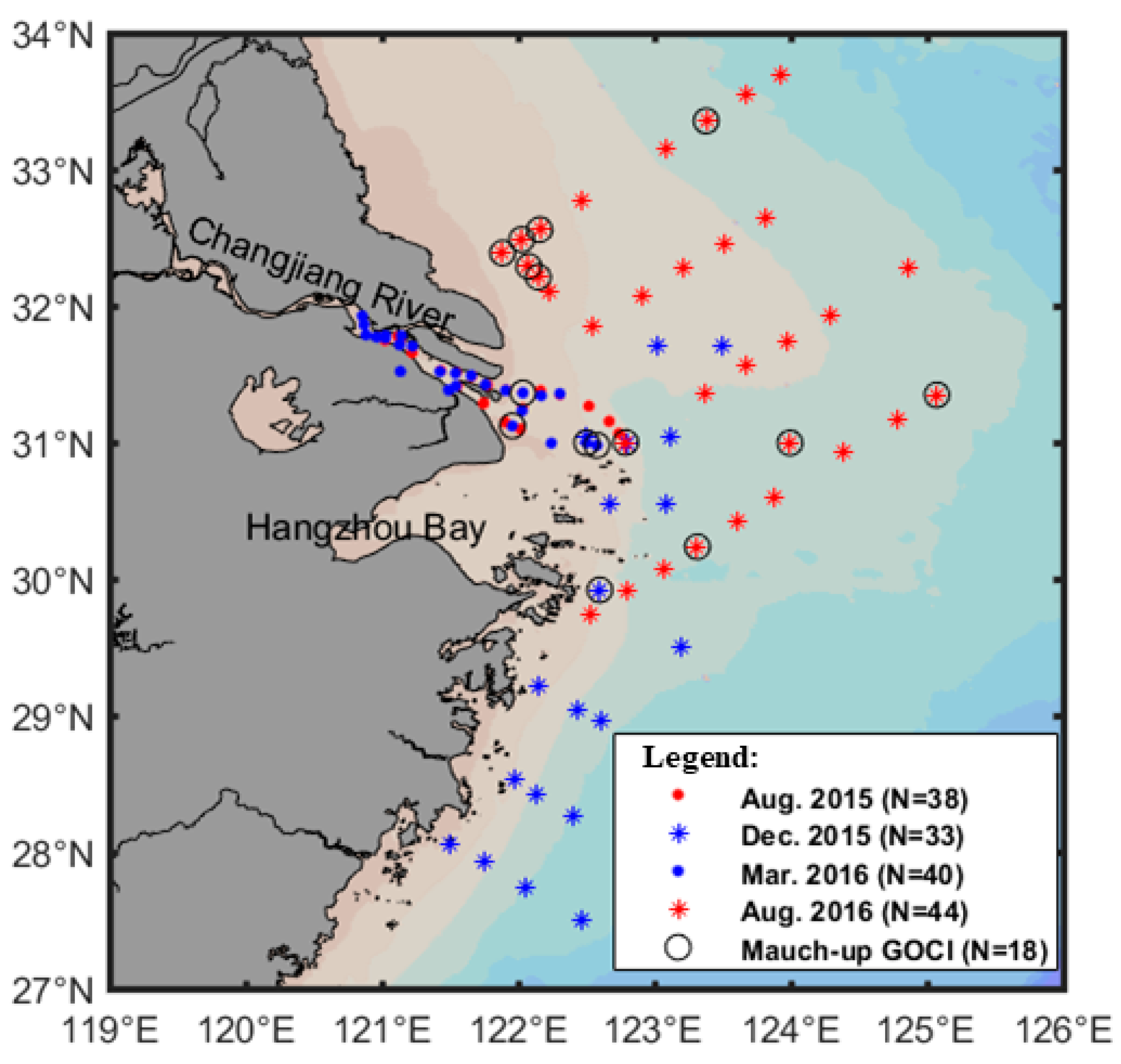
Four cruises were conducted in the Changjiang Estuary and ECS from 2015 to 2016 (Figure 2), including cruises in the wet season (August 2015) and dry season (March 2016) in the Changjiang Estuary, and two cruises (December 2015 and August 2016) on the shelf of the ECS. A total of 193 surface water samples were collected at a depth of 0.5 m with Niskin samplers. Salinity was measured with a handheld conductivity meter. Other water quality parameters, including chlorophyll, suspended matter, and nutrients, were obtained by laboratory measurement after filtering on the boat.
Nutrient samples were filtered with 0.45-μm cellulose acetate membranes, poisoned with 1–2% chloroform, and then frozen and kept at −20 °C for nitrate and phosphate measurements [22]. In the laboratory, nutrients were measured with an AA3 Auto-Analyzer following the methods of Han et al. [23]. Chlorophyll samples were filtered with glass-fiber membranes (0.7 μm pore size) and stored frozen in liquid nitrogen before measurement. In the laboratory, each filter was analyzed with a Turner-Design 10 fluorometer to obtain chlorophyll concentrations [24].
2.2.2. Measuring Remote-Sensing Reflectance
Remote-sensing reflectance (Rrs) was measured on board the ship using an ASD FieldSpec Spectroradiometer with a spectral range of 350–2500 nm (Analytical Spectral Devices Incorporation, ASD, Boulder, CO, USA). The upward radiance from the sea surface (Lt), standard reflecting plate (Lp), and downward sky radiance (Lsky) were measured at daytime stations with suitable light conditions. To avoid sun-glint, the zenith and azimuth angles of the probe were kept at about 40° and 135°, respectively. Additionally, we also selected the suitable locations to minimize the effects of ship shadow, foam, and floating objects [11]. Rrs was calculated as follows:
where βp and βs are the standard plate and air–sea interface reflectance, respectively. Then, Rrs needs to be converted to an equivalent reflectance (Rrs_equi) for direct comparison with satellite data [25]:
where Rrs_equi(λ) is the equivalent reflectance for a band with a central wavelength of λ, f(λ) is the spectral response function, F(λ) is the solar irradiance at a mean earth–sun distance, and λmin and λmax take values of 300 nm and 1000 nm, respectively.
2.3. Satellite Data
Rrs data from GOCI were used in this study. GOCI has eight spectral bands in the visible and near-infrared range, with central wavelengths of 412 nm, 443 nm, 490 nm, 555 nm, 660 nm, 680 nm, 745 nm, and 865 nm (Bands 1 to 8, or B1 to B8, respectively, in the ensuing paragraphs). GOCI regularly obtains eight images per day over the ECS from 8:30 a.m. to 3:30 p.m. local time, at a rate of once per hour. Level-2A data, which include the normalized water-leaving radiance (NLW), were obtained from the Korea Ocean Satellite Center (KOSC). NLW can be converted to Rrs by dividing by F(λ).
SSS was a key component of the model used in this study. Salinity data from the Soil Moisture Active Passive (SMAP) satellite were obtained. SMAP is an Earth satellite mission that measures and maps Earth’s soil moisture and SSS. SMAP has excellent spatial and temporal resolution (eight-day repetitive observations with a spatial resolution of 1/4°) compared with previous microwave radiometers, such as Soil Moisture and Ocean Salinity (SMOS) and Aquarius. Eight-day average data and monthly average data were obtained for April 2015 (when SMAP first released data) to December 2017 from the National Aeronautics and Space Administration (NASA) OPeNDAP website (https://opendap.jpl.nasa.gov/opendap/SalinityDensity/smap/L3/RSS/V2/monthly).
2.4. Artificial Neural Network
In coastal regions, the relationships between nutrients, salinity, chlorophyll, and TSM are very complex, and analytical models and semi-analytical models, which require solutions to radiation transfer equations, have difficulty obtaining exact solutions. Therefore, empirical models are often used to obtain the elements in Case II waters.
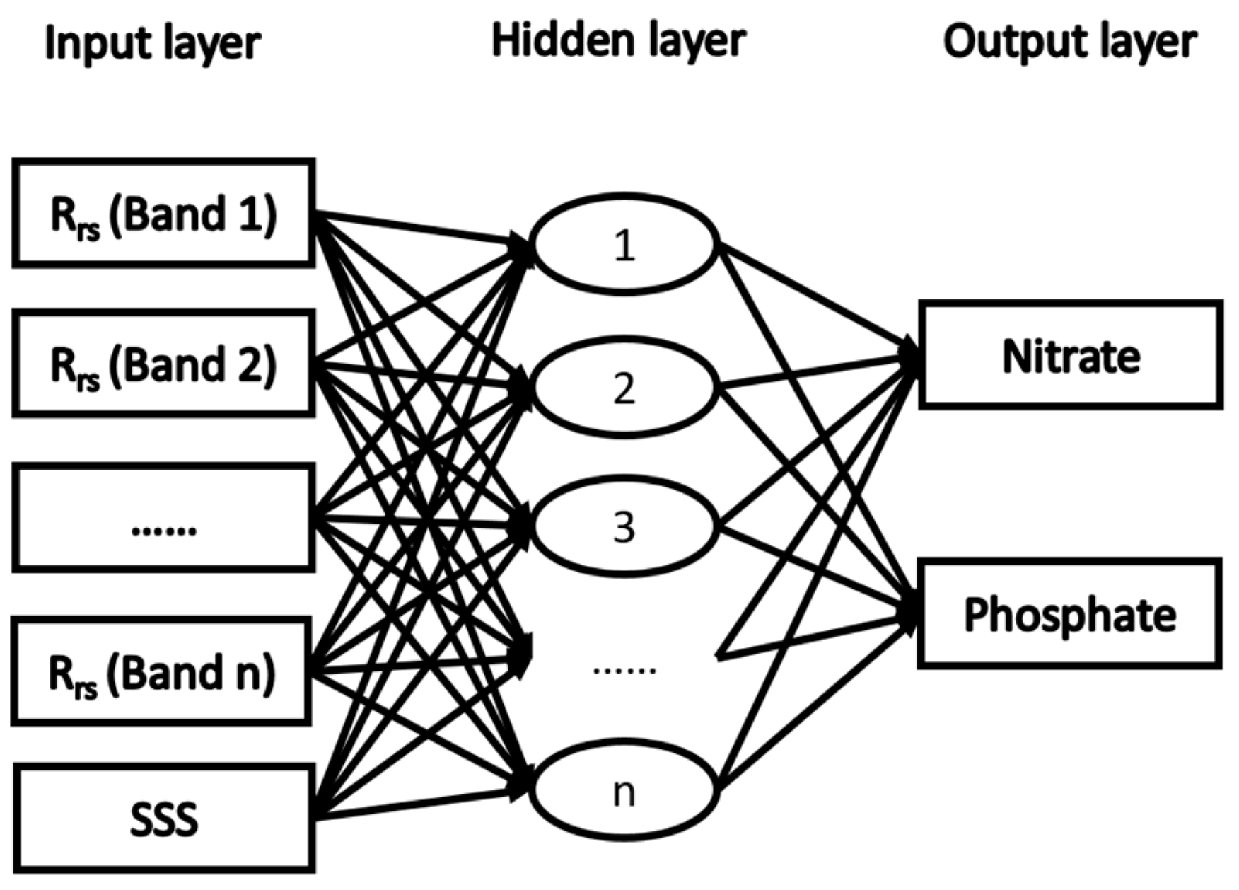
In this study, a back-propagation neural network (BP-NN) algorithm was applied to estimate the concentration of nitrate and phosphate in the surface water of the ECS. The network has three layers: the input layer, which distributes the input parameters; a hidden layer, where several neurons are contained; and the output layer, which distributes the target parameter. A neural network with a single hidden layer has the ability to simulate any nonlinearity [26]. The three-layer neural network used in this study is shown in Figure 3. In a BP-NN model, the information moves forward from the input nodes through the hidden nodes and to the output nodes. The back-propagation method was used in the network to calculate the gradient and adjust the weight of the neurons.
3. Developed Satellite Retrieval Models for Nutrients
3.1. Correlation between Nutrients and Rrs or SSS
Table 1 provides the coefficient of determination (R2) for the relationships between nutrients and in situ Rrs for each GOCI band. Both the nitrate and phosphate clearly have good relationships with the Rrs at long wavelengths, with the highest R2 being 0.68 and 0.67 for Band 5 (660 nm) for nitrate and phosphate, respectively. Overall, Rrs is useful for estimating concentrations of nutrients in the study area.
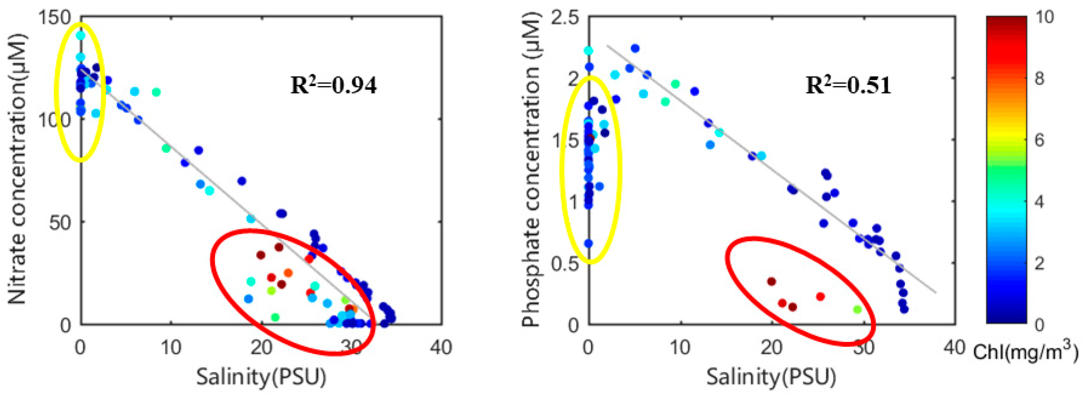
Figure 4 presents the relationship between nutrients and salinity. The values of R2 were 0.94 and 0.51 for nitrate and phosphate, respectively. In the moderate salinity range (SSS = 5–20 psu), nutrients behaved conservatively. However, there are some points that were lower than the conservative line in the continental shelf waters (SSS > 20), which may be due to the absorption of phytoplankton. Additionally, for phosphate, there are also some points below the conservative line in the inner river waters (SSS around 0). This may be due to adsorption and buffering by suspended sediment in the high-turbidity Changjiang River water [27,28]. Furthermore, it is clear that high chlorophyll concentrations were associated with low nitrate and phosphate concentrations at many shelf stations (Figure 4); in these cases, quantifying the influences on Rrs was important to the model. Therefore, in coastal regions influenced by large rivers, both Rrs and SSS are important for retrieving nutrients.
3.2. Training and Validation of the Neural Network
The MATLAB neural network toolbox (MathWorks, Natick, MA, USA) was used to build the BP-NN model for nitrate and phosphate. To eliminate the impact of dimensionality on the model, each parameter was scaled to (−1, 1). The initial weights related to nodes were created randomly at first, and the Levenberg–Marquardt algorithm was used for model training [29].
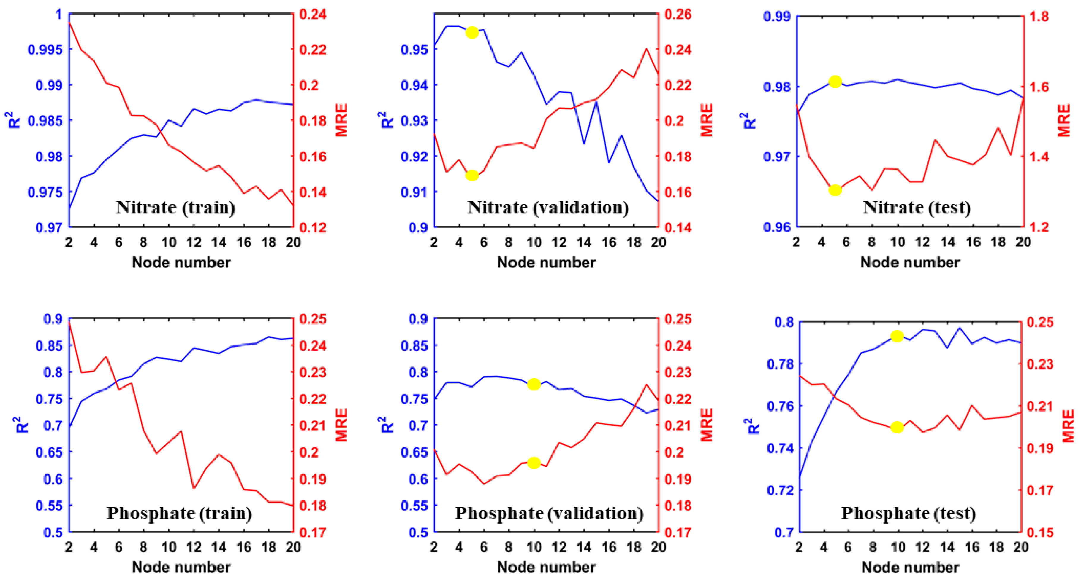
The number of hidden layer nodes, m, as a key parameter in the network, needs to be determined. The most suitable value of m varies with the complexity of the problem, and overfitting or undesirability occurs when m is too large or too small. To determine the optimal number of hidden nodes, training was performed with the value of m varying from 2 to 20. Figure 5 shows the changes in R2 and mean relative error (MRE) with different nodes. In each case, we averaged the results of 500 trainings to increase the model stability. The nitrate model reached steady state quickly. With an m value of 5, R2 exceeded 0.98, and remained almost unchanged with increases in m. MRE shows the opposite trend; when m was set to 5, the MRE for the nitrate network was marked as minimum, which shows that the accuracy was higher. The phosphate model was more complicated, and more nodes were needed; R2 and MRE achieved stability when m was set to 10. Additionally, the phosphate model was not as accurate as the nitrate model (Figure 5).
In situ Rrs_equi and SSS were used as input parameters to the BP-NN models, and nitrate and phosphate were target parameters. All in situ data were divided into three groups: 70% (135 samples) were used for model training; 15% (29 samples) were used for validation; and the remaining 15% (29 samples) were used for testing.
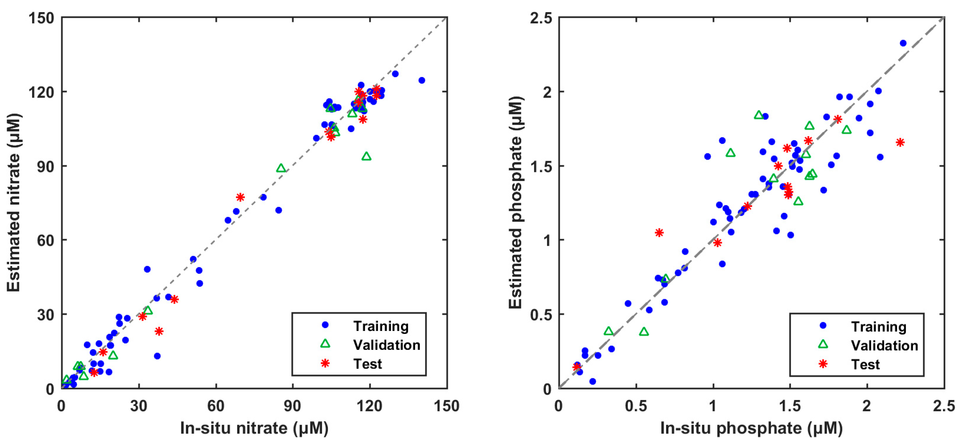
Figure 6 shows a comparison between model outputs and measured values; the R2, root-mean-square error (RMSE), and MRE values are presented in Table 2. The two models worked well in the study area using both SSS and spectral data as model inputs. Overall, the nitrate model was superior to the phosphate model, although both performed well. For nitrate, the R2, RMSE, and MRE between the inversion results and measured data were 0.99, 6.13 μM, and 11.2%, respectively; for phosphate, the R2, RMSE, and MRE were 0.83, 0.22 μM, and 13.7%, respectively.
4. Results
4.1. Evaluation of Satellite-Retrieved Rrs
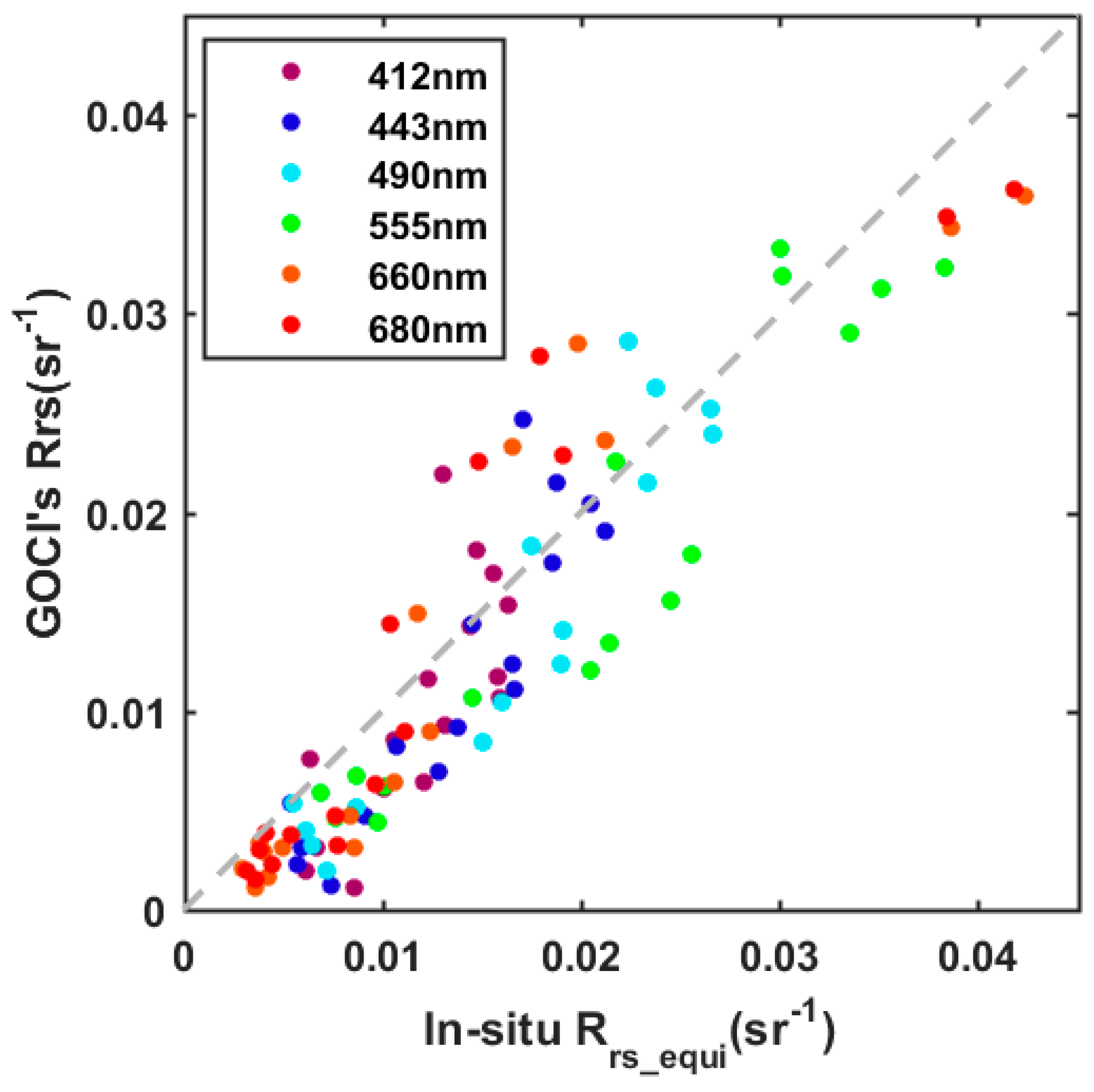
Atmospheric correction is one of the most important tasks for ocean color remote sensing in coastal waters. GOCI’s standard atmospheric correction algorithm is based on the method of Wang and Gordon (1994) [30]. To verify the suitability of GOCI’s Level-2 products in the study area, 18 sets of measured Rrs_equi synchronized with satellite data were chosen (Figure 2). The comparisons of measured Rrs_equi and satellite Rrs at these sites are presented in Figure 7, and Table 3 lists the R2, RMSE, and MRE from GOCI Band 1 to Band 6. The results for Band 1 (412 nm) were not as good as for other channels (R2 = 0.57). This is consistent with the observation that complete water absorption in the near-infrared range is questionable in turbid waters, and atmospheric correction products for the short-wave channel are inaccurate [31,32]. In contrast, the R2, RMSE, and MRE for the other five channels were acceptable for further research. Overall, the standard atmospheric correction algorithm of GOCI performed well in the study area.
4.2. Evaluation of Satellite-Measured Salinity
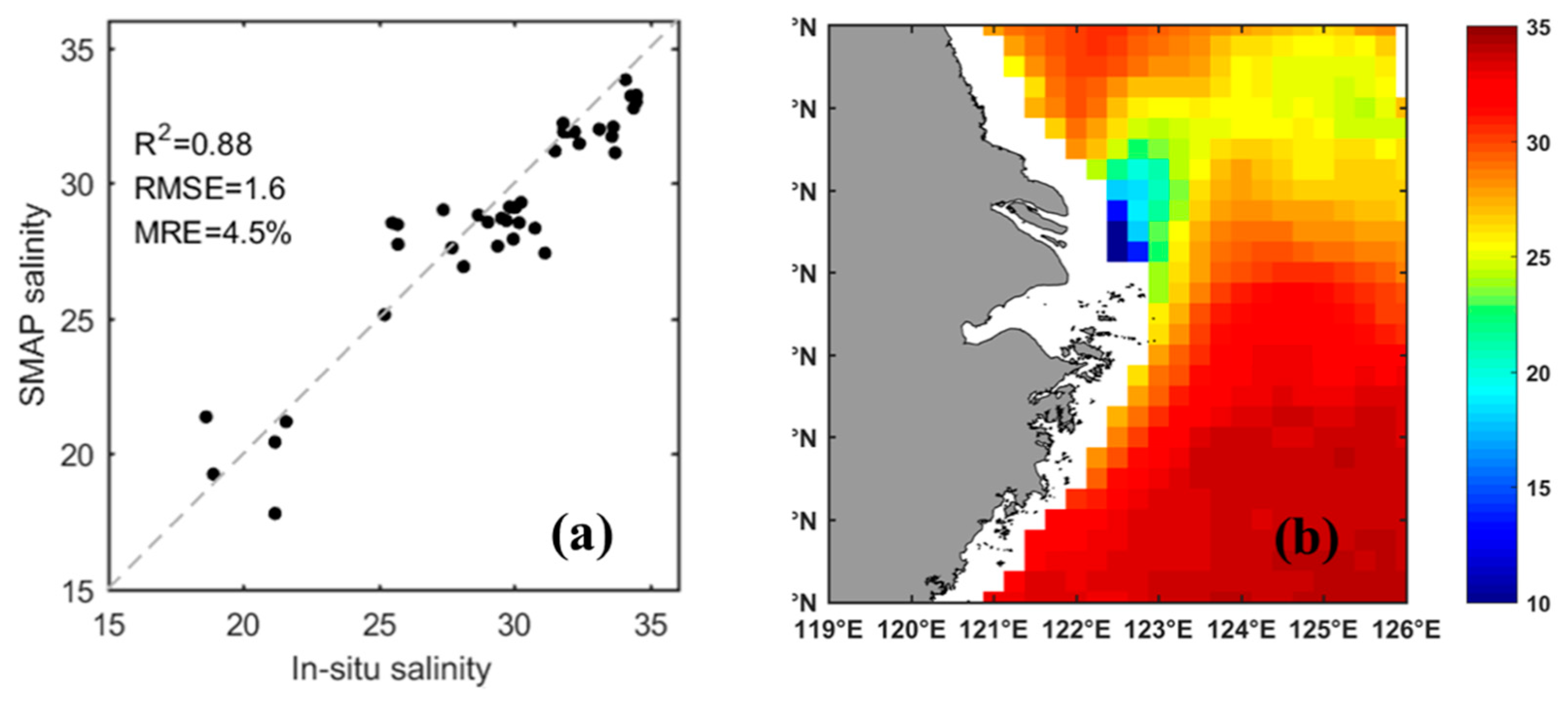
The SSS data of SMAP were compared with measured salinity. These two types of data showed good agreement, with R2 and MRE values of 0.88 and 4.5%, respectively (Figure 8a). However, there were some deficiencies in the SMAP data. Firstly, although SMAP has a higher spatial resolution (about 1/4°) than previous microwave radiometers, such as SMOS and Aquarius, it is still coarse compared with optical satellites that have spatial resolutions better than 1 km. In this study, SMAP data were converted to the same resolution as GOCI using optimal interpolation to allow combination with optical data. Moreover, terrestrial noises reduce the accuracy of the microwave radiometer, and in turn result in data deficiency in coastal areas, such as the Changjiang Estuary, Hangzhou Bay, and Zhejiang offshore waters.
4.3. Satellite-Derived Monthly Variations in Nutrients
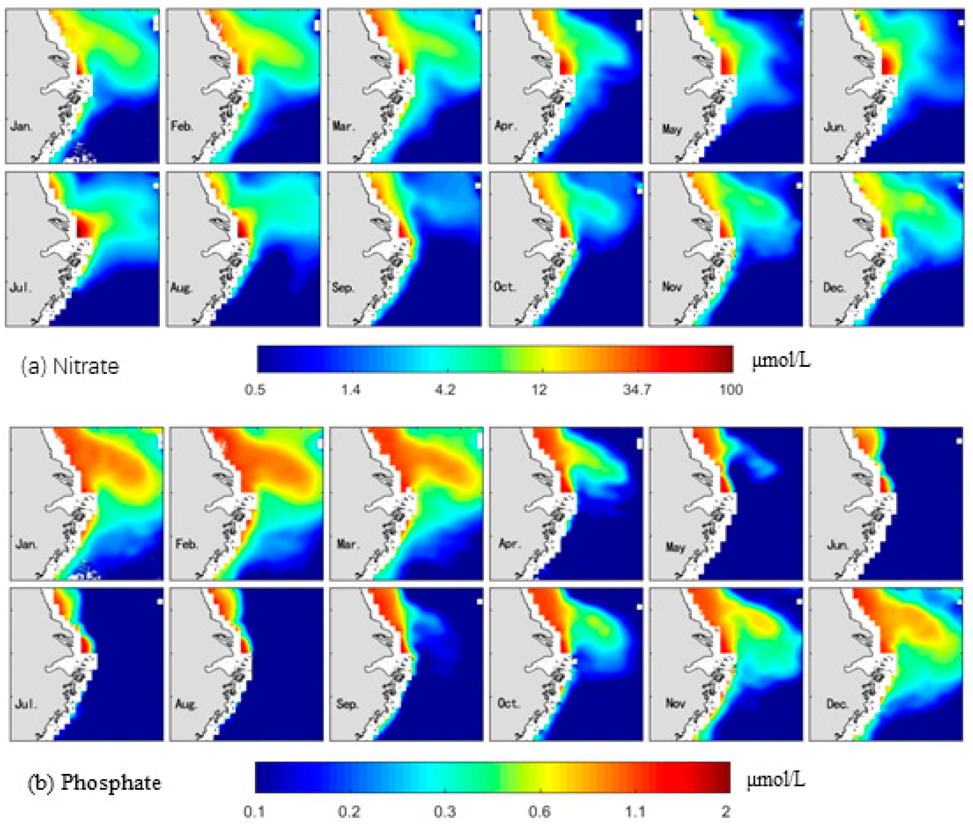
Monthly distributions of nitrate and phosphate concentrations were obtained with monthly satellite data as model inputs, followed by averaging from 2015 to 2017; the results are shown in Figure 9. It is clear that nutrient concentrations in the ECS were significantly affected by the Changjiang River plume, and there was a rapid declining trend from the nearshore to outer shelf.
Additionally, an eastward plume was found in the Changjiang Estuary, which intensified during the winter and summer, and weakened during the spring and autumn. In the winter (December to February), the sea surface water was forced by a strong northeasterly wind, and the nutrient-rich coastal water was widely spread to the outer shelf. Concurrently, due to low water temperatures and insufficient light levels in the winter, the consumption of nitrogen and phosphate by phytoplankton was limited, resulting in high nutrient concentrations on the shelf. In the spring and summer (April to September), significant amounts of nitrate and phosphate in the continental shelf waters were consumed with the increase in primary productivity. Phosphate, as the limiting factor in the ECS, was consumed more significantly than nitrate in the continental shelf, especially in the spring and summer [33].
5. Discussion
5.1. Comparison with Spectrum-Based Algorithms
In this study, BP-NN models were proposed to estimate the concentration of nitrate and phosphate in surface water using both satellite SSS data and optical data as input parameters. Prior to this study, there were two main methods for estimating the concentrations of nutrients. Firstly, global- or basin-scale models were employed based on the relationship between nutrients, sea surface temperature (SST), and chlorophyll concentration [34,35,36]. However, such models are not applicable to coastal waters, because there is little change in environmental elements, such as SST, on a small spatial scale. Secondly, regional models with satellite spectra as inputs were used [14,5]. These models are primarily based on the complex relationship between nutrients and satellite spectra and are suitable for closed and semi-closed aquatic systems; however, they have little utility in the ECS because of the completely different environment. Some studies analyzed the conservative characteristics of nutrients in larger river estuaries [16,17], while few studies focused on remote-sensing applications. There are various reasons for this lack of research. Firstly, it is difficult to obtain timely spatial SSS data. Prior to SMAP, salinity-sensing satellites (SMOS and Aquarius) with coarse spatial resolution could not meet the requirements for observing nearshore waters. Numerical simulations are another way of obtaining SSS; however, they are invalid in offshore waters because of low accuracy. The insufficiency of SSS data made it difficult to employ SSS-based nutrient models in the ECS. Secondly, Rrs and SSS are two different types of data, both having complex relationships with nutrients, and the traditional band ratio models and linear regressions are unsatisfactory for handling this complexity. In this study, the BP-NN algorithm was used to perform nonlinear fitting.
In Figure 10, we separately used SSS and GOCI spectra as input parameters to obtain four models, referred to as SSS-based models and spectrum-based models, respectively. These models were then compared with the previous mixed models. As mentioned previously, the conservative behavior of nutrients in the study area resulted in the good performance in the medium salinity range of SSS-based models. However, in the estuary and open sea, the SSS-based models were insufficient. The spectrum-based model, when used as a supplement, can correct the described defects; however, their overall precision is low. The mixed models using a combination of SSS and GOCI spectra as input parameters provide optimal results compared to the models using SSS and reflectance spectra alone.
5.2. Factors Impacting Nutrient Distributions
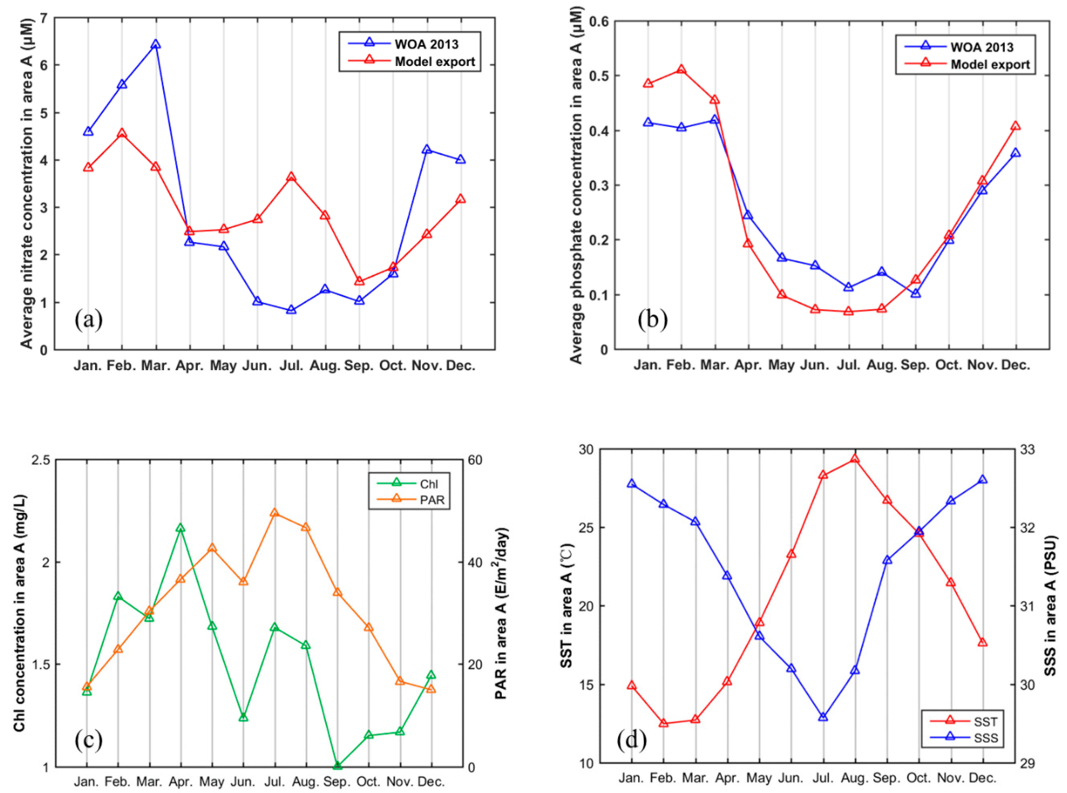
To further evaluate the model outputs, the monthly average results from 2015 to 2017 were calculated and compared with World Ocean Atlas nutrient data (WOA13, V2) [37]. WOA13 is a reanalysis data set published by the National Oceanic and Atmospheric Administration (NOAA) which includes the global monthly mean nitrate and phosphate concentrations with 1° resolution based on measured data. As WOA13 is also insufficient in nearshore waters, we chose Zone A (Figure 1) as representative, and averaged the nutrient concentrations in Zone A to obtain monthly changes. As shown in Figure 11a,b, overall, the trends of our model result and those of WOA13 are similar; the nitrate and phosphate in the study area were characterized by high concentrations in the winter and low concentrations in the summer. Furthermore, the nutrients decreased significantly after April because of the increase in primary productivity. Some differences were found for nitrate concentration; for example, there is an upward trend in the BP-NN estimates from June to July due to the strengthening Changjiang River plume that the WOA13 data do not capture due to poor data coverage for near-coast waters. Additionally, phosphate rather than nitrate is the limiting factor in the ECS [38], which results in greater absorption of phosphate in the spring and summer compared to nitrate.
River inputs, precipitation, and exchanges between water masses are major sources of nutrients in coastal waters [39,40,41]. Primary production, adsorption, and sedimentation are the main mechanisms for transferring nutrients and sea surface currents, and the resuspension of sediment in shallow waters caused by wind and tide also affects the distribution of nutrients [42,43]. The average nitrate concentrations measured on our two Changjiang Estuary cruises were 114.8 ± 11.0 μM and 104.7 ± 20.7 μM, respectively, and the average phosphate concentrations were 1.35 ± 0.39 μM and 1.48 ± 0.28 μM, respectively. Therefore, the concentrations of nitrate and phosphate discharged by the Changjiang River were the same in the dry season and the wet season. That is, the nutrient flux, i.e., the amount of transported nutrients, is directly proportional to river run-off.
The ECS is a typical subtropical shelf sea with clear seasonal variations in precipitation, solar radiation, and temperature. To analyze the environmental factors related to nutrient changes, the satellite-derived monthly chlorophyll, photosynthetically active radiation (PAR), and sea surface temperature (SST) from 2015 to 2017 were evaluated. These data, at 9-km resolution, were estimated based on the Visible Infrared Imaging Radiometer Suite (VIIRS) obtained from the NASA OceanColor website (https://oceancolor.gsfc.nasa.gov/). The monthly changes in these elements are shown in Figure 11c,d. Surface nutrient concentrations are clearly negatively related to chlorophyll, PAR, and SST, and are positively related to SSS, in the study area.
The changes in nutrient concentrations compared with environmental variables in different seasons are presented in Table 4. During the winter (December to February), the concentrations of nitrate and phosphate were lower, and reached a minimum in December before gradually trending upward. Concurrently, precipitation (a factor in SSS) and PAR also increased monthly during the winter, which indicates that the terrestrial input of nutrients dominates sea surface nutrients during winter.
River flow continued growing in the spring (March to May); however, phosphate concentrations began declining because of the increase in PAR and primary productivity. In contrast, changes in nitrate were not stable. Nitrate decreased in early spring and then increased after April, indicating that nitrate concentration in the spring was jointly dominated by terrestrial input and phytoplankton uptake.
During the summer (June to August), photosynthesis continued increaseing, and phosphates on the continental shelf were almost exhausted, with an average concentration of less than 0.1 μM. However, nitrate remained rich due to abundant sources from the river.
During the autumn (September to November), both river discharge and primary productivity decreased; however, the concentration of nitrate and phosphate increased. There are two reasons for this observation: (1) the reduction in primary productivity led to a decrease in nutrient consumption; (2) wind-induced resuspension resulted in nutrients in the sediment being carried into the surface waters.
6. Conclusions
Satellite retrieval models of surface water nitrate and phosphate concentrations based on back-propagation neural networks were developed for coastal regions in the ECS. The conservative behaviors of nitrate and phosphate were discussed, and the relationships between nutrients, Rrs, salinity, and chlorophyll were analyzed. We used both SSS and Rrs as model inputs. After training and validation with a large amount of measured data, reliable models were obtained. Level-2 Rrs data from GOCI and SSS data from SMAP were compared with in situ data; both showed good agreement, which indicated their applicability to the study area. Based on these models, time-series monthly variations in nitrate and phosphate concentrations for 2015–2017 were obtained for the first time. The spatial characteristics and monthly changes in nutrients were analyzed further, and the results were found to be consistent with WOA13 data.
Nitrate and phosphate are important water quality indicators in coastal waters. Remote-sensing monitoring methods can provide large-scale, high-frequency observations, and this study is a contribution to addressing this issue in complex coastal waters. Moreover, our study emphasizes that salinity is an important parameter in developing satellite retrieval models for nutrients in large river-dominated marginal seas.
Author Contributions
Conceptualization, D.W. and X.H. Methodology, D.W. and Q.C. Software, Q.C. and D.W. Validation, Y.B., Q.C., and D.W. Resources, F.G. and L.W. Data curation, Q.C. Writing—original draft preparation, Q.C. and D.W. Writing—review and editing, X.H. and Y.B. Supervision, D.W. Project administration, D.W. Funding acquisition, D.W.
Funding
This study was supported by the National Key R&D Program of China (No. 2017YFC1405300), the National Basic Research Programme (“973” Programme) of China (No. 2015CB954002), the key research and development plan of Zhejiang Province under contract No. 2017C03037, the National Natural Science Foundation of China (Nos. 41476157,L1624046, 41676170, 41676172, and 41621064) and the Special Program of the Second Institute of Oceanography under Grant No. JT1404.
Acknowledgments
We thank the Laboratory of Marine Environmental Science (MEL) of Xiamen University for the excellent in situ nutrient data. We also thank the satellite ground station and the satellite data processing and sharing center of SOED/SIO for help with the data processing. All authors would like to thank the reviewers for their detailed and critical comments and helpful suggestions.
Conflicts of Interest
The authors declare no conflict of interest.
References
- Feng, S.Z.; Li, F.Q.; Li, S.J. Introduction to Oceanography; Higher Education Press: Beijing, China, 1999. [Google Scholar]
- Chai, C.; Yu, Z.; Song, X.; Cao, X. The Status and Characteristics of Eutrophication in the Yangtze River (Changjiang) Estuary and the Adjacent East China Sea, China. Hydrobiologia 2006, 563, 313–328. [Google Scholar] [CrossRef]
- Hautier, Y.; Hector, A. Competition for Light Causes Plant Biodiversity Loss after Eutrophication. Science 2009, 324, 636–638. [Google Scholar] [CrossRef] [PubMed] [Green Version]
- Heisler, J.; Glibert, P.M.; Burkholder, J.M.; Anderson, D.M.; Cochlan, W.; Dennison, W.C.; Dortch, Q.; Gobler, C.J.; Heil, C.A.; Humphries, E.; et al. Eutrophication and Harmful Algal Blooms: A Scientific Consensus. Harmful Algae 2008, 8, 3–13. [Google Scholar] [CrossRef] [PubMed]
- Chang, N.B.; Xuan, Z.; Yang, Y.J. Exploring spatiotemporal patterns of phosphorus concentrations in a coastal bay with MODIS images and machine learning models. Remote Sens. Environ. 2013, 134, 100–110. [Google Scholar] [CrossRef]
- Yu, X.; Yi, H.; Liu, X.; Wang, Y.; Liu, X.; Zhang, H. Remote-sensing estimation of dissolved inorganic nitrogen concentration in the Bohai Sea using band combinations derived from MODIS data. Int. J. Remote Sens. 2016, 37, 327–340. [Google Scholar] [CrossRef] [Green Version]
- Kassi, J.-B.; Racault, M.-F.; Mobio, B.A.; Platt, T.; Sathyendranath, S.; Raitsos, D.E.; Affian, K. Remotely Sensing the Biophysical Drivers of Sardinella aurita Variability in Ivorian Waters. Remote Sens. 2018, 10, 785. [Google Scholar] [CrossRef]
- Pan, J.; Huang, L.; Devlin, A.T.; Lin, H. Quantification of Typhoon-Induced Phytoplankton Blooms Using Satellite Multi-Sensor Data. Remote Sens. 2018, 10, 318. [Google Scholar] [CrossRef]
- Markogianni, V.; Kalivas, D.; Petropoulos, G.P.; Dimitriou, E. An Appraisal of the Potential of Landsat 8 in Estimating Chlorophyll-a, Ammonium Concentrations and Other Water Quality Indicators. Remote Sens. 2018, 10, 1018. [Google Scholar] [CrossRef]
- Choi, J.K.; Park, Y.J.; Ahn, J.H.; Lim, H.S.; Eom, J.; Ryu, J.H. GOCI, the world’s first geostationary ocean color observation satellite, for the monitoring of temporal variability in coastal water turbidity. J. Geophys. Res. Oceans 2012, 117, C09004. [Google Scholar] [CrossRef]
- He, X.; Bai, Y.; Pan, D.; Huang, N.; Dong, X.; Chen, J.; Chen, C.T.; Cui, Q. Using geostationary satellite ocean color data to map the diurnal dynamics of suspended particulate matter in coastal waters. Remote Sens. Environ. 2013, 133, 225–239. [Google Scholar] [CrossRef]
- Mobley, C.D. Light and Water: Radiative Transfer in Natural Waters; Academic Press: San Diego, CA, USA, 1994. [Google Scholar]
- Brodie, J.; Schroeder, T.; Rohde, K.; Faithful, J.; Masters, B.; Dekker, A.; Brando, V.; Maughan, M. Dispersal of suspended sediments and nutrients in the Great Barrier Reef lagoon during river-discharge events: Conclusions from satellite remote sensing and concurrent flood-plume sampling. Mar. Freshw. Res. 2010, 61, 651–664. [Google Scholar] [CrossRef]
- Huang, C.; Guo, Y.; Yang, H.; Li, Y.; Zou, J.; Zhang, M.; Lyu, H.; Zhu, A.; Huang, T. Using remote sensing to track variation in phosphorus and its interaction with chlorophyll-a and suspended sediment. IEEE J. Sel. Top. Appl. Earth Obs. Remote Sens. 2015, 8, 4171–4180. [Google Scholar] [CrossRef]
- Huang, Y.; Fan, D.; Liu, D.; Song, L.; Ji, D.; Hui, E. Nutrient estimation by HJ-1 satellite imagery of Xiangxi Bay, Three Gorges Reservoir, China. Environ. Earth Sci. 2016, 75, 633. [Google Scholar] [CrossRef]
- Edmond, J.M.; Boyle, E.A.; Grant, B.; Stallard, R.F. The chemical mass balance in the Amazon plume I: The nutrients. Deep Sea Res. Part A Oceanogr. Res. Pap. 1981, 28, 1339–1374. [Google Scholar] [CrossRef]
- Zhang, J. Nutrient elements in large Chinese estuaries. Cont. Shelf Res. 1996, 16, 1023–1045. [Google Scholar] [CrossRef]
- Changjiang Water Resources Commission. Changjiang Sediment Bulletin 2016. Available online: http://www.cjw.gov.cn/UploadFiles/zwzc/2018/8/201808271416045463.pdf (accessed on 30 September 2018). (In Chinese)
- Tong, Y.; Bu, X.; Chen, J.; Zhou, F.; Chen, L.; Liu, M.; Tan, X.; Yu, T.; Zhang, W.; Mi, Z.; et al. Estimation of nutrient discharge from the Yangtze River to the East China Sea and the identification of nutrient sources. J. Hazard. Mater. 2017, 321, 728–736. [Google Scholar] [CrossRef] [PubMed]
- Luo, X.; Wei, H.; Liu, Z.; Zhao, L. Seasonal variability of air–sea CO2 fluxes in the Yellow and East China Seas: A case study of continental shelf sea carbon cycle model. Cont. Shelf Res. 2015, 107, 69–78. [Google Scholar] [CrossRef]
- Li, H.; Kang, X.; Li, X.; Li, Q.; Song, J.; Jiao, N.; Zhang, Y. Heavy metals in surface sediments along the weihai coast, china: Distribution, sources and contamination assessment. Mar. Pollut. Bull. 2017, 115, 551–558. [Google Scholar] [CrossRef] [PubMed]
- Wang, G.; Wang, S.; Wang, Z.; Jing, W.; Xu, Y.; Zhang, Z.; Tan, E.; Dai, M. Tidal variability of nutrients in a coastal coral reef system influenced by groundwater. Biogeosciences 2018, 15, 997–1009. [Google Scholar] [CrossRef] [Green Version]
- Han, A.; Dai, M.; Kao, S.J.; Gan, J.; Li, Q.; Wang, L.; Zhai, W.; Wang, L. Nutrient dynamics and biological consumption in a large continental shelf system under the influence of both a river plume and coastal upwelling. Limnol. Oceanogr. 2012, 57, 486–502. [Google Scholar] [CrossRef] [Green Version]
- Bai, Y.; Pan, D.; Cai, W.J.; He, X.; Wang, D.; Tao, B.; Zhu, Q. Remote sensing of salinity from satellite-derived CDOM in the Changjiang River dominated East China Sea. J. Geophys. Res. Oceans 2013, 118, 227–243. [Google Scholar] [CrossRef] [Green Version]
- Liu, D.; Pan, D.; Bai, Y.; He, X.; Wang, D.; Wei, J.A.; Zhang, L. Remote sensing observation of particulate organic carbon in the Pearl River Estuary. Remote Sens. 2015, 7, 8683–8704. [Google Scholar] [CrossRef]
- Keiner, L.E. Estimating oceanic chlorophyll concentrations with neural networks. Int. J. Remote Sens. 1999, 20, 189–194. [Google Scholar] [CrossRef]
- Pomero, L.R.; Smith, E.E.; Grant, C.M. The exchange of phosphate between estuarine water and sediments. Limnol. Oceanogr. 1965, 10, 167–172. [Google Scholar]
- Mayer, L.M.; Gloss, S.P. Buffering of silica and phosphate in a turbid river. Limnol. Oceanogr. 1980, 25, 12–22. [Google Scholar] [CrossRef] [Green Version]
- Zhang, Y.; Pulliainen, J.; Koponen, S.; Hallikainen, M. Application of an empirical neural network to surface water quality estimation in the Gulf of Finland using combined optical data and microwave data. Remote Sens. Environ. 2002, 81, 327–336. [Google Scholar] [CrossRef]
- Wang, M.; Gordon, H.R. A simple, moderately accurate, atmospheric correction algorithm for seawifs. Remote Sens. Environ. 1994, 50, 231–239. [Google Scholar] [CrossRef]
- He, X.; Bai, Y.; Pan, D.; Tang, J.; Wang, D. Atmospheric correction of satellite ocean color imagery using the ultraviolet wavelength for highly turbid waters. Opt. Express 2012, 20, 20754–20770. [Google Scholar] [CrossRef] [PubMed]
- Oo, M.; Vargas, M.; Gilerson, A.; Gross, B.; Moshary, F.; Ahmed, S. Improving atmospheric correction for highly productive coastal waters using the short wave infrared retrieval algorithm with water-leaving reflectance constraints at 412 nm. Appl. Opt. 2008, 47, 3846–3859. [Google Scholar] [CrossRef] [PubMed]
- Wang, B.D.; Wang, X.L.; Zhan, R. Nutrient conditions in the Yellow Sea and the East China Sea. Estuar. Coast. Shelf Sci. 2003, 58, 127–136. [Google Scholar] [CrossRef]
- Arteaga, L.; Pahlow, M.; Oschlies, A. Global monthly sea surface nitrate fields estimated from remotely sensed sea surface temperature, chlorophyll, and modeled mixed layer depth. Geophys. Res. Lett. 2015, 42, 1130–1138. [Google Scholar] [CrossRef] [Green Version]
- Sarangi, R.K. Remote-sensing-based estimation of surface nitrate and its variability in the southern peninsular Indian waters. Int. J. Oceanogr. 2012, 2011, 172731. [Google Scholar] [CrossRef]
- Switzer, A.C.; Kamykowski, D.; Zentara, S.J. Mapping nitrate in the global ocean using remotely sensed sea surface temperature. J. Geophys. Res. Oceans 2003, 108, 3280. [Google Scholar] [CrossRef]
- Garcia, H.E.; Locarnini, R.A.; Boyer, T.P.; Antonov, J.I.; Baranova, O.K.; Zweng, M.M.; Reagan, J.R.; Johnson, D.R. World Ocean Atlas 2013, Volume 4: Dissolved Inorganic Nutrients (Phosphate, Nitrate, Silicate); NOAA Atlas NESDIS 76: Silver Spring, MD, USA, 2014; 25p. Available online: https://data.nodc.noaa.gov/woa/WOA13/DOC/woa13_vol4.pdf (accessed on 30 September 2018).
- Wang, B.D. Nutrient distributions and their limitation of phytoplankton in the Yellow Sea and the East China Sea. J. Appl. Ecol. 2003, 14, 1122–1126. (In Chinese) [Google Scholar]
- Anderson, D.M.; Glibert, P.M.; Burkholder, J.M. Harmful algal blooms and eutrophication: Nutrient sources, composition, and consequences. Estuaries 2002, 25, 704–726. [Google Scholar] [CrossRef]
- Carpenter, S.R.; Caraco, N.F.; Correll, D.L.; Howarth, R.W.; Sharpley, A.N.; Smith, V.H. Nonpoint pollution of surface waters with phosphorus and nitrogen. Ecol. Appl. 1998, 8, 559–568. [Google Scholar] [CrossRef]
- Paerl, H.W. Coastal eutrophication and harmful algal blooms: Importance of atmospheric deposition and groundwater as “new” nitrogen and other nutrient sources. Limnol. Oceanogr. 1997, 42, 1154–1165. [Google Scholar] [CrossRef] [Green Version]
- Fanning, K.A.; Carder, K.L.; Betzer, P.R. Sediment resuspension by coastal waters: A potential mechanism for nutrient re-cycling on the ocean’s margins. Deep Sea Res. Part A. Oceanogr. Res. Pap. 1982, 29, 953–965. [Google Scholar] [CrossRef]
- Shi, X.; Wang, X.; Han, X.; Zhu, C.; Sun, X.; Zhang, C. Nutrient distribution and its controlling mechanism in the adjacent area of Changjiang River estuary. J. Appl. Ecol. 2003, 14, 1086–1092. (In Chinese) [Google Scholar]
Figure 1.
Bathymetry and regional ocean circulations in the study area. The arrows indicate the Changjiang Diluted Water (CDW), Yellow Sea Warm Current (YSWC), SuBei Coastal Current (SBCC), Zhejiang–Fujian Coastal Current (ZFCC), and Taiwan Warm Current (TWC) [20,21]. The red dashed box is Zone A (122.5–125.5°E, 27.5–33.5°N), where the regional average was calculated for comparison with WOA13 data (detailed in Section 5.2).

Figure 2.
Locations of sampling sites. Two Changjiang Estuary cruises were conducted in August 2015 and March 2016, and two continental shelf cruises were conducted in December 2015 and August 2016. Black circles indicate the sites where the weather was clear during sampling and synchronous satellite observations were obtained.

Figure 3.
The three-layer neural network used in this study. In this study, the nitrate and phosphate networks were trained separately using in situ data.
Figure 3.
The three-layer neural network used in this study. In this study, the nitrate and phosphate networks were trained separately using in situ data.

Figure 4.
Relationships between in situ salinity and the concentration of nutrients. The color of the points represents chlorophyll concentration. Points circled in red indicate sites where nitrate and phosphate concentrations were significantly lower than conservative lines in high-salinity waters. Points circled in yellow indicate phosphate concentrations in the estuarine freshwater that are significantly lower than the conservative line.

Figure 5.
Variation in coefficient of determination (R2; blue lines) and mean relative error (MRE; red lines) with the number of hidden nodes in the nitrate and phosphate networks. Yellow dots indicate the point when the model achieved stability.
Figure 5.
Variation in coefficient of determination (R2; blue lines) and mean relative error (MRE; red lines) with the number of hidden nodes in the nitrate and phosphate networks. Yellow dots indicate the point when the model achieved stability.

Figure 6.
Comparisons of in situ samples and model estimates for nitrate and phosphate. The training, validation, and test data are represented by different symbols.
Figure 6.
Comparisons of in situ samples and model estimates for nitrate and phosphate. The training, validation, and test data are represented by different symbols.

Figure 7.
Evaluation of Level-2 data of the Geostationary Ocean Color Imager (GOCI). The colors of points represent different GOCI bands.
Figure 7.
Evaluation of Level-2 data of the Geostationary Ocean Color Imager (GOCI). The colors of points represent different GOCI bands.

Figure 8.
Evaluation of Soil Moisture Active Passive (SMAP) data. (a) Comparison of measured sea surface salinity (SSS) with matching SMAP products. (b) Monthly average SSS of SMAP in August 2016.
Figure 8.
Evaluation of Soil Moisture Active Passive (SMAP) data. (a) Comparison of measured sea surface salinity (SSS) with matching SMAP products. (b) Monthly average SSS of SMAP in August 2016.

Figure 9.
Monthly average results for concentrations of nitrogen (a) and phosphate (b) in the Changjiang River plume in the ECS from 2015 to 2017.
Figure 9.
Monthly average results for concentrations of nitrogen (a) and phosphate (b) in the Changjiang River plume in the ECS from 2015 to 2017.

Figure 10.
Comparisons between different nutrient models using (a,b) sea surface salinity (SSS) as the input parameter (SSS-based model), (c,d) remote-sensing reflectance (Rrs) as the input parameter (spectrum-based model), and (e,f) combined SSS and Rrs as input parameters (mixed model).
Figure 10.
Comparisons between different nutrient models using (a,b) sea surface salinity (SSS) as the input parameter (SSS-based model), (c,d) remote-sensing reflectance (Rrs) as the input parameter (spectrum-based model), and (e,f) combined SSS and Rrs as input parameters (mixed model).

Figure 11.
(a,b) Comparisons of monthly average nutrient concentration from model estimates and the World Ocean Atlas data (WOA13, V2) in Zone A (Figure 1). (c,d) Monthly average changes in chlorophyll concentration, photosynthetically active radiation (PAR), sea surface temperature (SST), and sea surface salinity (SSS) in Zone A.


Table 1.
The coefficient of determination (R2) between nitrates, phosphates, and measured remote-sensing reflectance (Rrs) for each Geostationary Ocean Color Imager (GOCI) band (B).
Table 1.
The coefficient of determination (R2) between nitrates, phosphates, and measured remote-sensing reflectance (Rrs) for each Geostationary Ocean Color Imager (GOCI) band (B).
| B1 | B2 | B3 | B4 | B5 | B6 | |
|---|---|---|---|---|---|---|
| Nitrates | <0.1 | 0.27 | 0.37 | 0.58 | 0.68 | 0.66 |
| Phosphates | 0.13 | 0.37 | 0.50 | 0.67 | 0.67 | 0.64 |
Table 2.
The coefficient of determination (R2), root-mean-square error (RMSE), and mean relative error (MRE) between in situ and estimated nutrients. All measured data were divided into three groups for training, validation, and testing.
Table 2.
The coefficient of determination (R2), root-mean-square error (RMSE), and mean relative error (MRE) between in situ and estimated nutrients. All measured data were divided into three groups for training, validation, and testing.
| Nitrate | Phosphate | |||||
|---|---|---|---|---|---|---|
| R2 | RMSE | MRE | R2 | RMSE | MRE | |
| Training | 0.98 | 6.14 | 13.5% | 0.86 | 0.20 | 14.6% |
| Validation | 0.98 | 7.68 | 17.7% | 0.75 | 0.25 | 16.7% |
| Test | 0.99 | 6.13 | 11.2% | 0.83 | 0.22 | 13.3% |
| All | 0.98 | 6.38 | 13.8% | 0.84 | 0.21 | 14.7% |
Table 3.
The coefficient of determination (R2), root-mean-square error (RMSE), and mean relative error (MRE) between the Geostationary Ocean Color Imager (GOCI)’s Rrs and measured Rrs_equi in different bands.
Table 3.
The coefficient of determination (R2), root-mean-square error (RMSE), and mean relative error (MRE) between the Geostationary Ocean Color Imager (GOCI)’s Rrs and measured Rrs_equi in different bands.
| R2 | RMSE | MRE | |
|---|---|---|---|
| Band 1 (412 nm) | 0.57 | 0.0043 | 0.332 |
| Band 2 (443 nm) | 0.80 | 0.0040 | 0.299 |
| Band 3 (490 nm) | 0.87 | 0.0041 | 0.270 |
| Band 4 (555 nm) | 0.89 | 0.0052 | 0.251 |
| Band 5 (660 nm) | 0.89 | 0.0042 | 0.353 |
| Band 6 (680 nm) | 0.87 | 0.0043 | 0.336 |
Table 4.
Monthly average changes in nutrients and other related elements in Zone A. I (increase), D (decrease), and - (stable) describe the monthly changes. The interrelationships between changes in various factors should be noted. SSS—sea surface salinity; PAR—photosynthetically active radiation.
Table 4.
Monthly average changes in nutrients and other related elements in Zone A. I (increase), D (decrease), and - (stable) describe the monthly changes. The interrelationships between changes in various factors should be noted. SSS—sea surface salinity; PAR—photosynthetically active radiation.
| Winter | Spring | Summer | Autumn | |||||||||
|---|---|---|---|---|---|---|---|---|---|---|---|---|
| Dec. | Jan. | Feb. | Mar. | Apr. | May | Jun. | Jul. | Aug. | Sep. | Oct. | Nov. | |
| Nitrate | I | I | D | D | - | I | I | D | D | I | I | I |
| Phosphate | I | I | D | D | D | D | - | - | I | I | I | I |
| SSS | D | D | D | D | D | D | D | I | I | I | I | I |
| Flux | I | I | I | I | I | I | I | D | D | D | D | D |
| PAR | - | I | I | I | I | D | I | D | D | D | D | D |
© 2018 by the authors. Licensee MDPI, Basel, Switzerland. This article is an open access article distributed under the terms and conditions of the Creative Commons Attribution (CC BY) license (http://creativecommons.org/licenses/by/4.0/).
Share and Cite
MDPI and ACS Style
Wang, D.; Cui, Q.; Gong, F.; Wang, L.; He, X.; Bai, Y. Satellite Retrieval of Surface Water Nutrients in the Coastal Regions of the East China Sea. Remote Sens. 2018, 10, 1896. https://doi.org/10.3390/rs10121896
AMA Style
Wang D, Cui Q, Gong F, Wang L, He X, Bai Y. Satellite Retrieval of Surface Water Nutrients in the Coastal Regions of the East China Sea. Remote Sensing. 2018; 10(12):1896. https://doi.org/10.3390/rs10121896
Chicago/Turabian StyleWang, Difeng, Qiyuan Cui, Fang Gong, Lifang Wang, Xianqiang He, and Yan Bai. 2018. "Satellite Retrieval of Surface Water Nutrients in the Coastal Regions of the East China Sea" Remote Sensing 10, no. 12: 1896. https://doi.org/10.3390/rs10121896
Note that from the first issue of 2016, this journal uses article numbers instead of page numbers. See further details here.