A Comparison of Imputation Approaches for Estimating Forest Biomass Using Landsat Time-Series and Inventory Data

 , , and
Abstract
:
1. Introduction
2. Materials and Methods
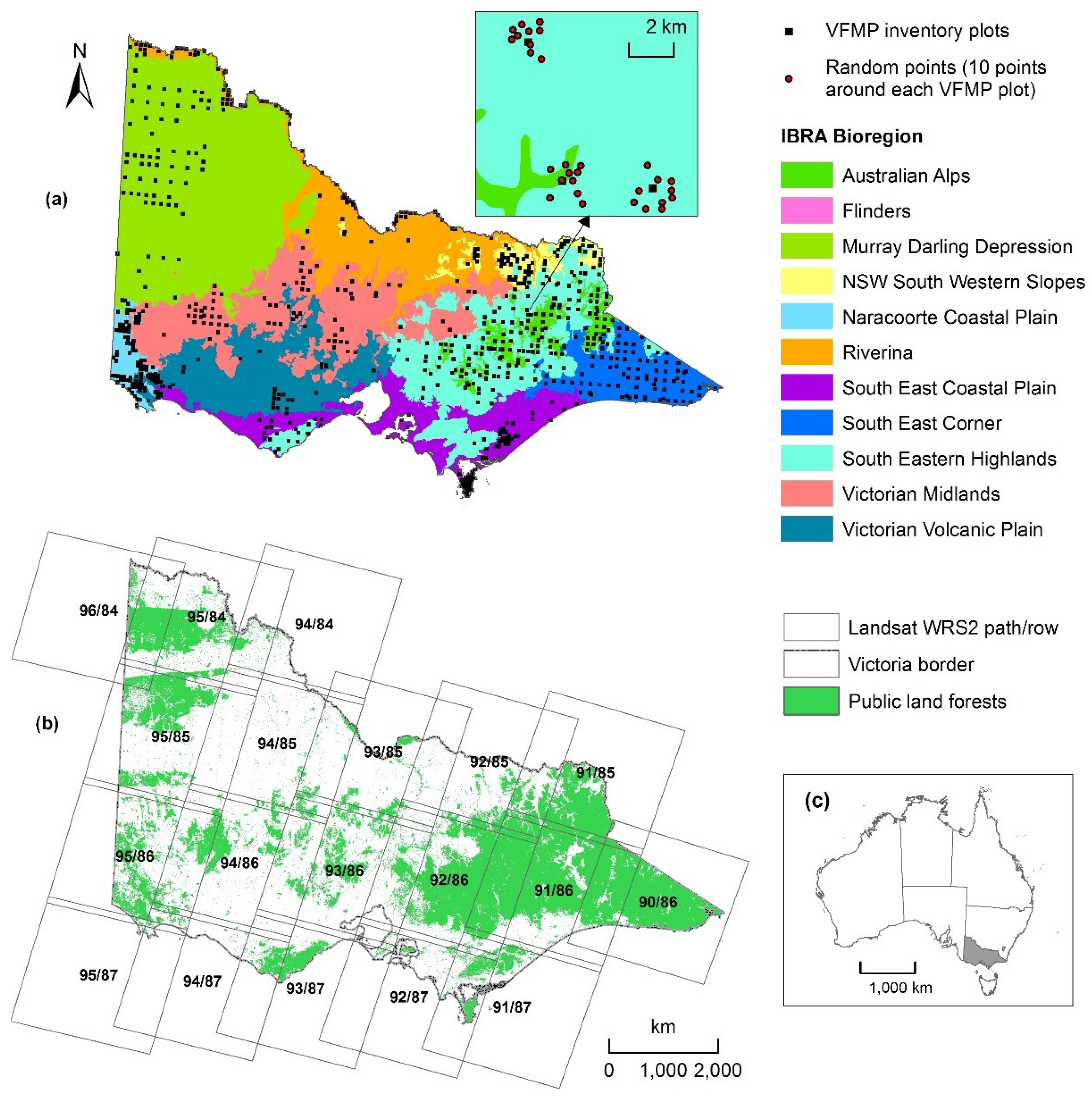
2.1. Study Area
2.2. Forest Biomass and Structure Response Variables
2.3. Predictor Variables
2.3.1. Landsat Time-Series
2.3.2. Topographic and Climatic Ancillary Data
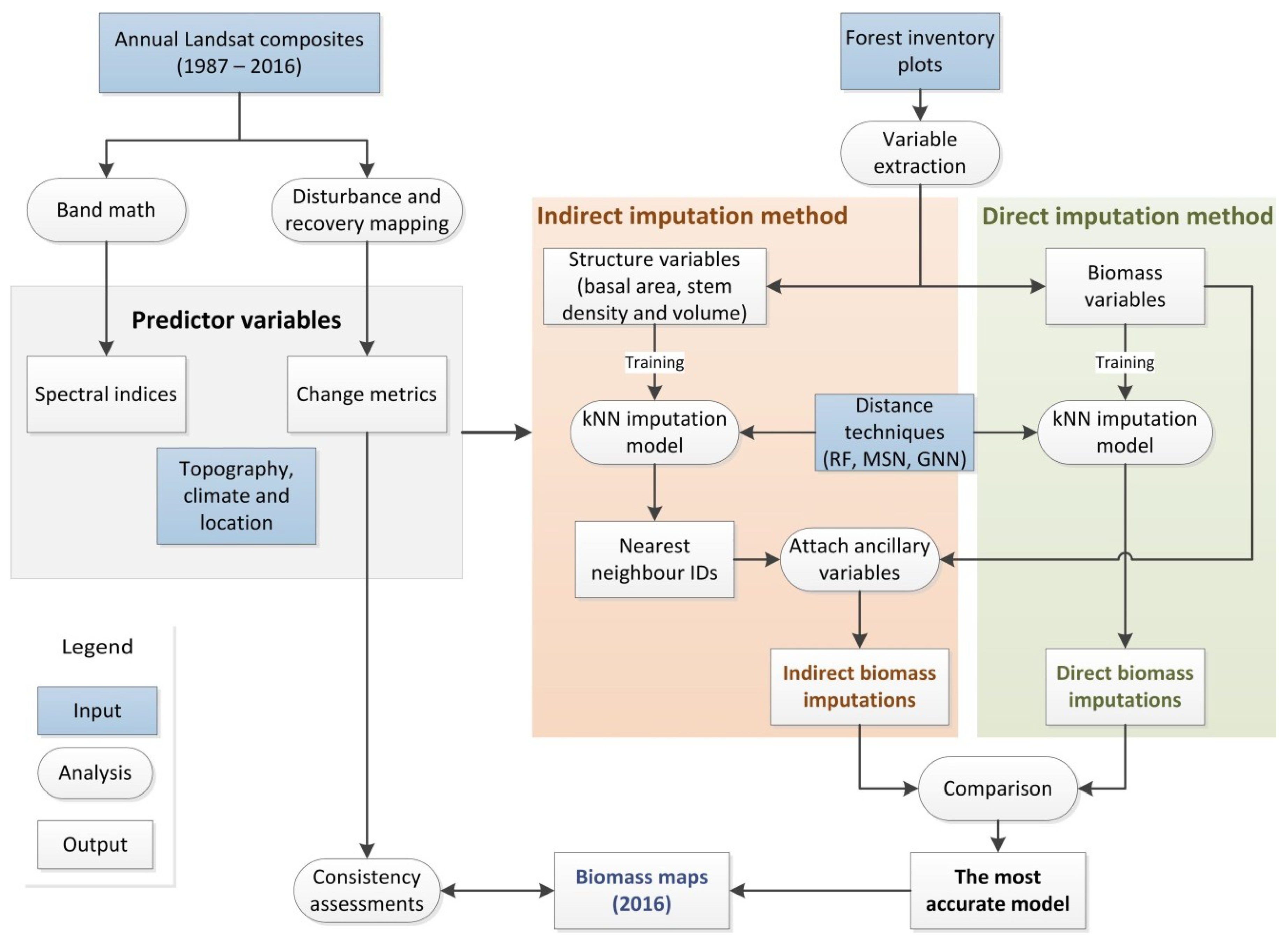
2.4. Biomass Model Development
2.4.1. Variable Extraction
2.4.2. Variable Selection
2.4.3. Imputation Models
2.4.4. Model Evaluation
2.4.5. Assessment of Biomass Imputation Maps Using Disturbance History
3. Results
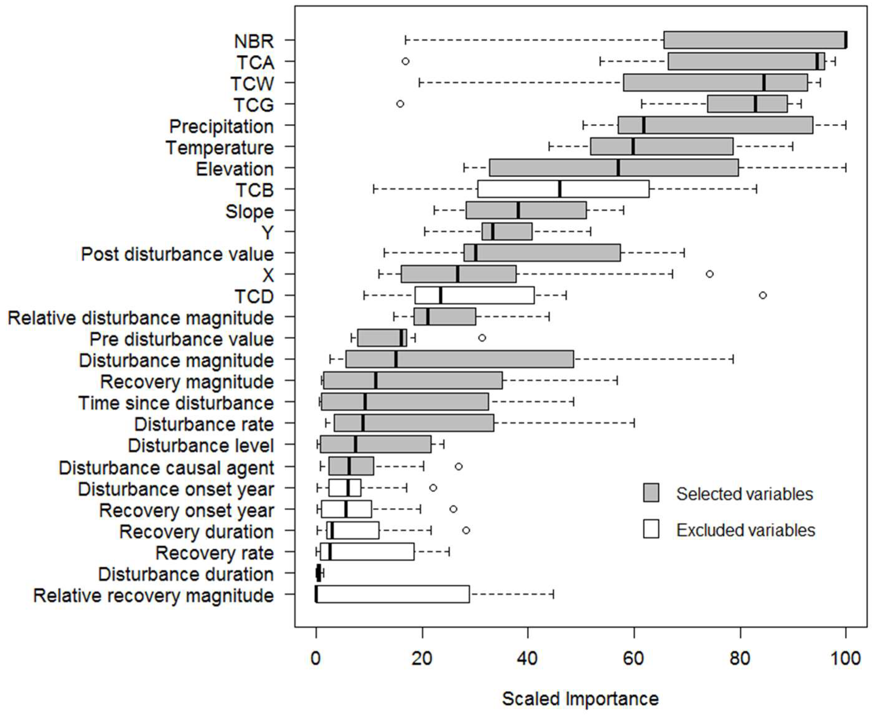
3.1. Variable Selection
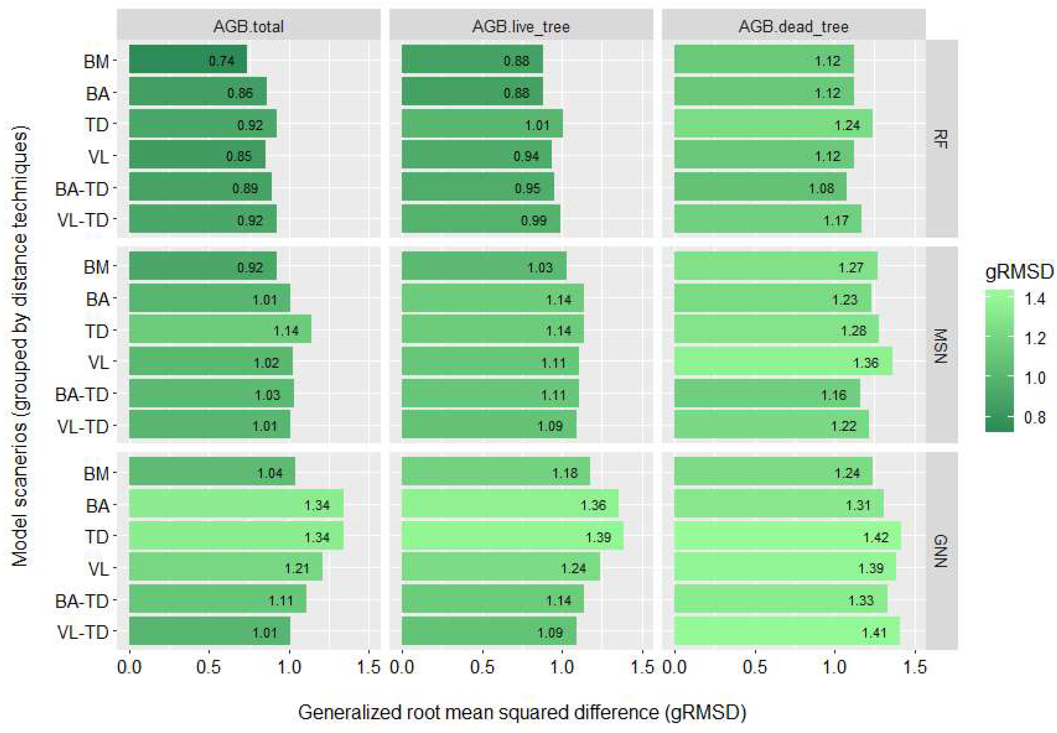
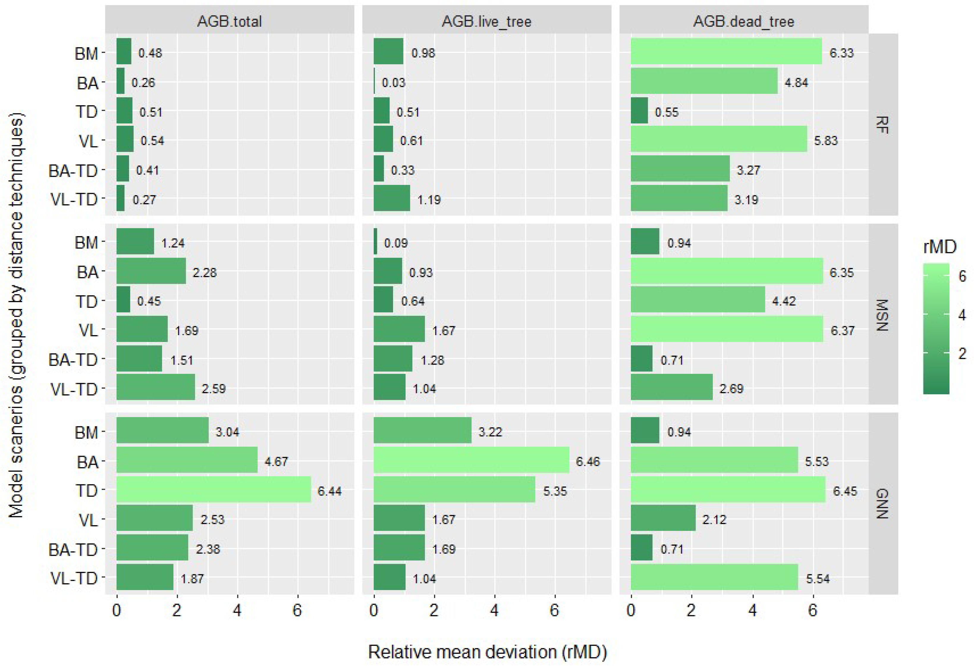
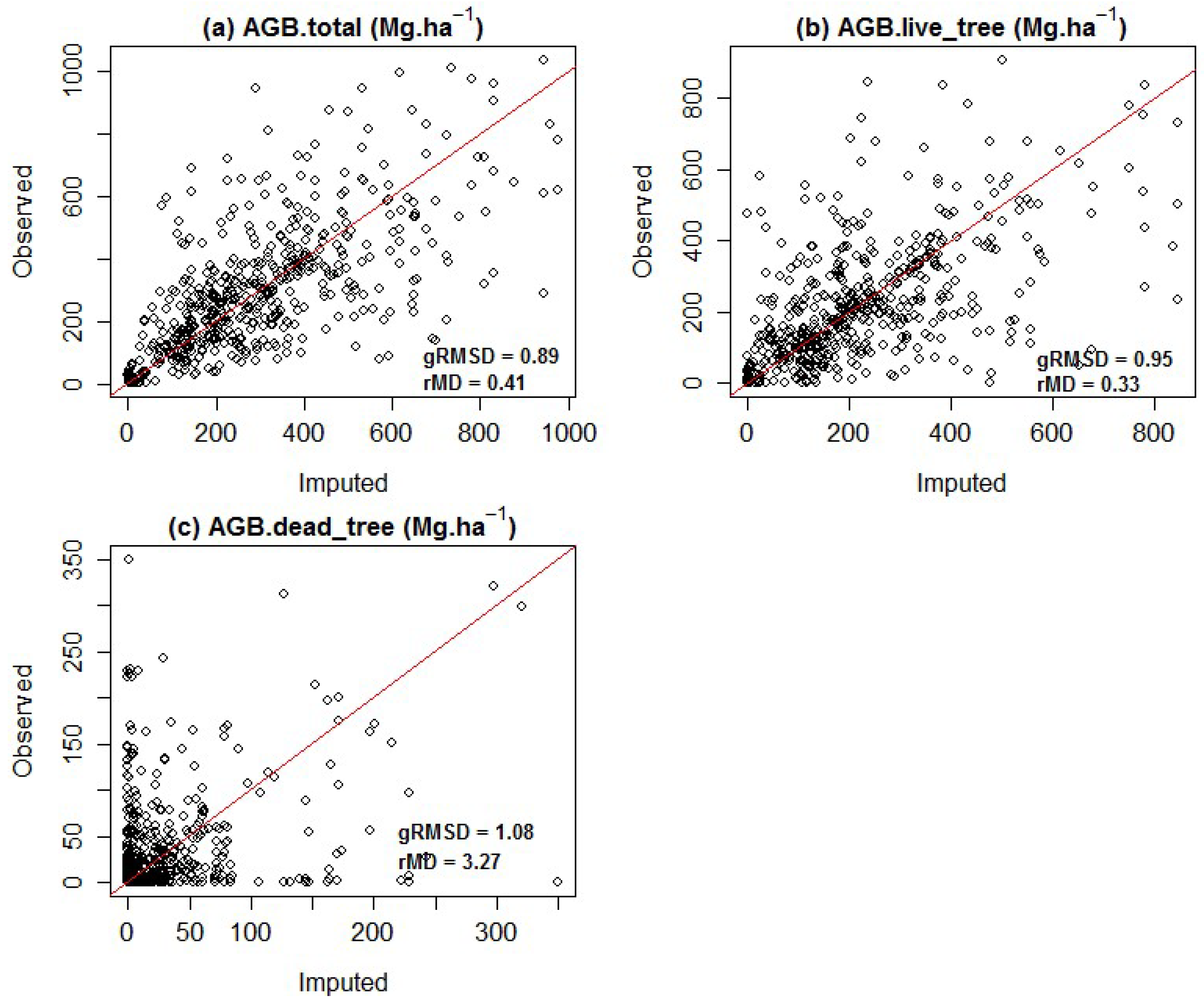
3.2. Biomass Imputation Model Accuracy
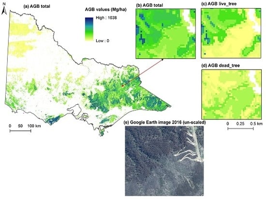
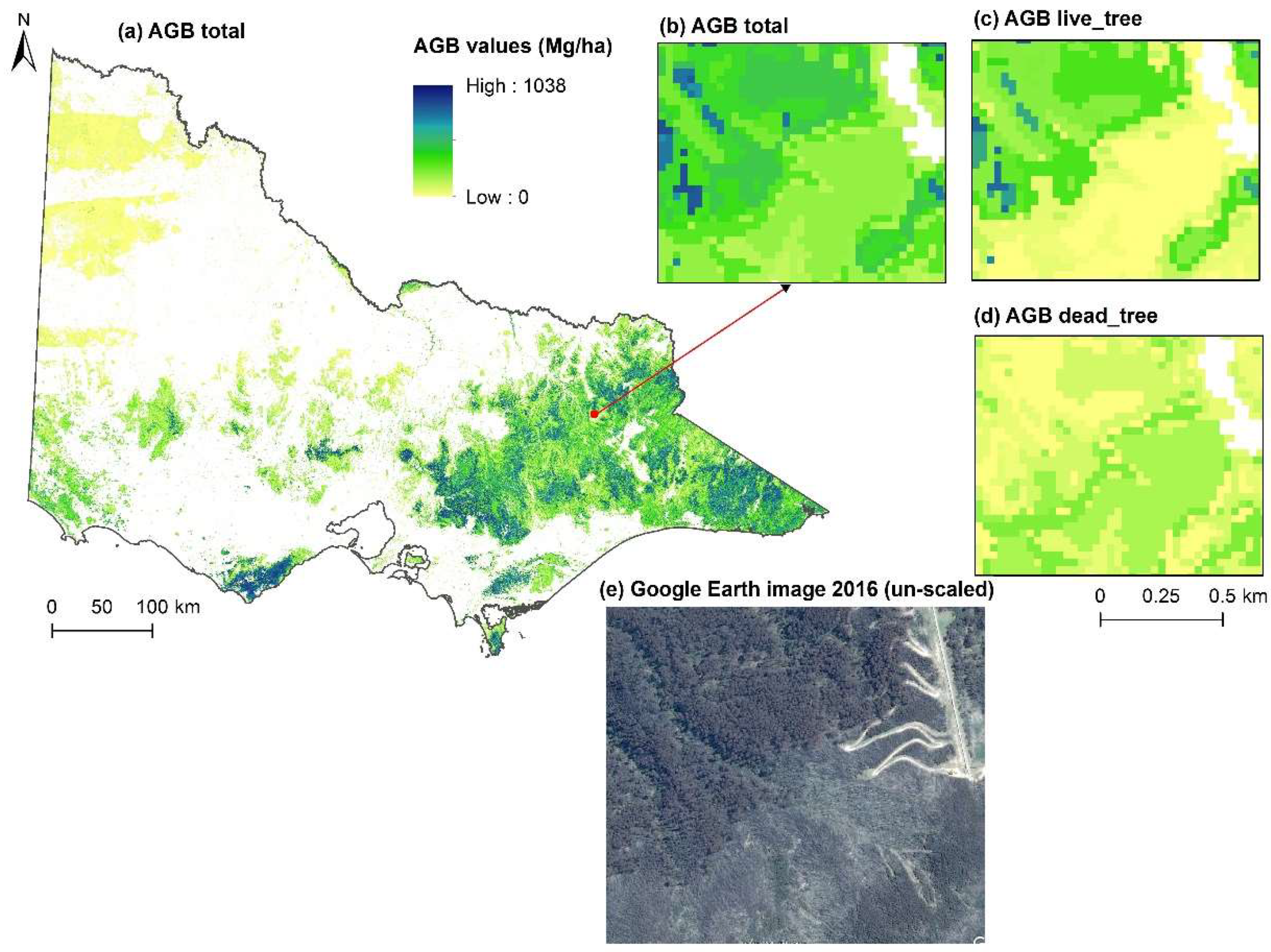
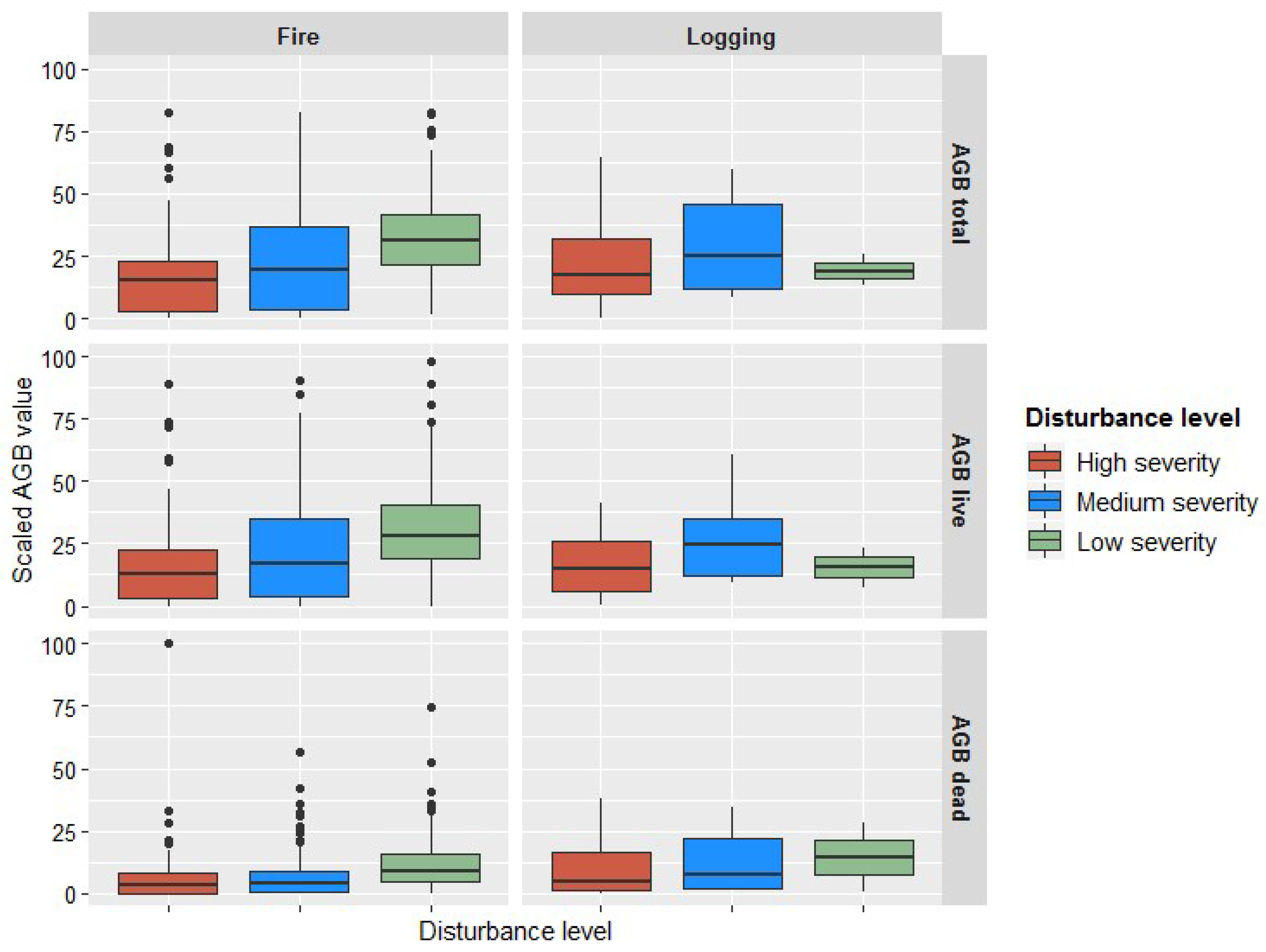
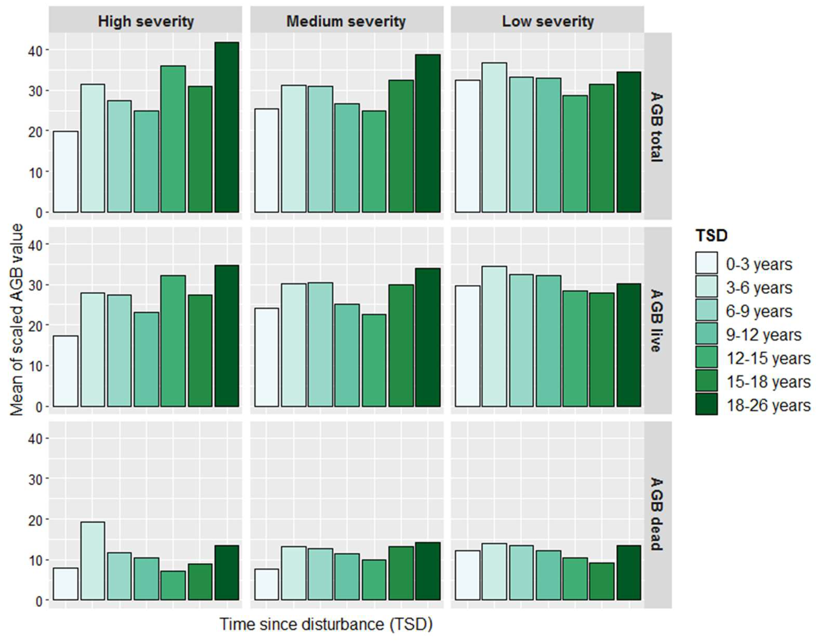
3.3. Biomass Imputation Maps in Relation to Disturbance History
4. Discussion
5. Conclusions
Author Contributions
Funding
Acknowledgments
Conflicts of Interest
References
- Houghton, R.A.; Hall, F.; Goetz, S.J. Importance of biomass in the global carbon cycle. J. Geophys. Res. Biogeosci. 2009, 114. [Google Scholar] [CrossRef] [Green Version]
- Tomppo, E.; Olsson, H.; Ståhl, G.; Nilsson, M.; Hagner, O.; Katila, M. Combining national forest inventory field plots and remote sensing data for forest databases. Remote Sens. Environ. 2008, 112, 1982–1999. [Google Scholar] [CrossRef]
- Wulder, M.; Skakun, R.; Kurz, W.; White, J. Estimating time since forest harvest using segmented Landsat ETM+ imagery. Remote Sens. Environ. 2004, 93, 179–187. [Google Scholar] [CrossRef]
- Cao, L.; Coops, N.C.; Innes, J.L.; Sheppard, S.R.J.; Fu, L.; Ruan, H.; She, G. Estimation of forest biomass dynamics in subtropical forests using multi-temporal airborne LiDAR data. Remote Sens. Environ. 2016, 178, 158–171. [Google Scholar] [CrossRef]
- Badreldin, N.; Sanchez-Azofeifa, A. Estimating Forest Biomass Dynamics by Integrating Multi-Temporal Landsat Satellite Images with Ground and Airborne LiDAR Data in the Coal Valley Mine, Alberta, Canada. Remote Sens. 2015, 7, 2832–2849. [Google Scholar] [CrossRef] [Green Version]
- Zald, H.S.J.; Ohmann, J.L.; Roberts, H.M.; Gregory, M.J.; Henderson, E.B.; McGaughey, R.J.; Braaten, J. Influence of lidar, Landsat imagery, disturbance history, plot location accuracy, and plot size on accuracy of imputation maps of forest composition and structure. Remote Sens. Environ. 2014, 143, 26–38. [Google Scholar] [CrossRef]
- Meyer, V.; Saatchi, S.S.; Chave, J.; Dalling, J.W.; Bohlman, S.; Fricker, G.A.; Robinson, C.; Neumann, M.; Hubbell, S. Detecting tropical forest biomass dynamics from repeated airborne lidar measurements. Biogeosciences 2013, 10, 5421–5438. [Google Scholar] [CrossRef]
- Tsui, O.W.; Coops, N.C.; Wulder, M.A.; Marshall, P.L.; McCardle, A. Using multi-frequency radar and discrete-return LiDAR measurements to estimate above-ground biomass and biomass components in a coastal temperate forest. ISPRS J. Photogramm. Remote Sens. 2012, 69, 121–133. [Google Scholar] [CrossRef]
- Pflugmacher, D.; Cohen, W.B.; Kennedy, R.E. Using Landsat-derived disturbance history (1972–2010) to predict current forest structure. Remote Sens. Environ. 2012, 122, 146–165. [Google Scholar] [CrossRef]
- Waser, L.; Ginzler, C.; Rehush, N. Wall-to-Wall Tree Type Mapping from Countrywide Airborne Remote Sensing Surveys. Remote Sens. 2017, 9. [Google Scholar] [CrossRef]
- He, Q.; Chen, E.; An, R.; Li, Y. Above-Ground Biomass and Biomass Components Estimation Using LiDAR Data in a Coniferous Forest. Forests 2013, 4, 984–1002. [Google Scholar] [CrossRef] [Green Version]
- Ioki, K.; Tsuyuki, S.; Hirata, Y.; Phua, M.-H.; Wong, W.V.C.; Ling, Z.-Y.; Saito, H.; Takao, G. Estimating above-ground biomass of tropical rainforest of different degradation levels in Northern Borneo using airborne LiDAR. Forest Ecol. Manag. 2014, 328, 335–341. [Google Scholar] [CrossRef]
- Wulder, M.A.; White, J.C.; Bater, C.W.; Coops, N.C.; Hopkinson, C.; Chen, G. Lidar plots—A new large-area data collection option: context, concepts, and case study. Can. J. Remote Sens. 2014, 38, 600–618. [Google Scholar] [CrossRef]
- White, J.C.; Coops, N.C.; Wulder, M.A.; Vastaranta, M.; Hilker, T.; Tompalski, P. Remote Sensing Technologies for Enhancing Forest Inventories: A Review. Can. J. Remote Sens. 2016, 42, 619–641. [Google Scholar] [CrossRef]
- Matasci, G.; Hermosilla, T.; Wulder, M.A.; White, J.C.; Coops, N.C.; Hobart, G.W.; Zald, H.S.J. Large-area mapping of Canadian boreal forest cover, height, biomass and other structural attributes using Landsat composites and lidar plots. Remote Sens. Environ. 2018, 209, 90–106. [Google Scholar] [CrossRef]
- Bolton, D.K.; White, J.C.; Wulder, M.A.; Coops, N.C.; Hermosilla, T.; Yuan, X. Updating stand-level forest inventories using airborne laser scanning and Landsat time series data. Int. J. Appl. Earth Observ. Geoinf. 2018, 66, 174–183. [Google Scholar] [CrossRef]
- Jiménez, E.; Vega, J.A.; Fernández-Alonso, J.M.; Vega-Nieva, D.; Ortiz, L.; López-Serrano, P.M.; López-Sánchez, C.A. Estimation of aboveground forest biomass in Galicia (NW Spain) by the combined use of LiDAR, LANDSAT ETM+ and National Forest Inventory data. iForest Biogeosci. For. 2017, 10, 590–596. [Google Scholar] [CrossRef]
- Deo, R.; Russell, M.; Domke, G.; Andersen, H.-E.; Cohen, W.; Woodall, C. Evaluating Site-Specific and Generic Spatial Models of Aboveground Forest Biomass Based on Landsat Time-Series and LiDAR Strip Samples in the Eastern USA. Remote Sens. 2017, 9, 598. [Google Scholar] [CrossRef]
- Zald, H.S.J.; Wulder, M.A.; White, J.C.; Hilker, T.; Hermosilla, T.; Hobart, G.W.; Coops, N.C. Integrating Landsat pixel composites and change metrics with lidar plots to predictively map forest structure and aboveground biomass in Saskatchewan, Canada. Remote Sens. Environ. 2016, 176, 188–201. [Google Scholar] [CrossRef]
- Pflugmacher, D.; Cohen, W.B.; Kennedy, R.E.; Yang, Z. Using Landsat-derived disturbance and recovery history and lidar to map forest biomass dynamics. Remote Sens. Environ. 2014, 151, 124–137. [Google Scholar] [CrossRef]
- Cohen, W.B.; Goward, S.N. Landsat’s role in ecological applications of remote sensing. Bioscience 2004, 54, 535–545. [Google Scholar] [CrossRef]
- Cohen, W.; Healey, S.; Yang, Z.; Stehman, S.; Brewer, C.; Brooks, E.; Gorelick, N.; Huang, C.; Hughes, M.; Kennedy, R.; et al. How Similar Are Forest Disturbance Maps Derived from Different Landsat Time Series Algorithms? Forests 2017, 8, 98. [Google Scholar] [CrossRef]
- Nguyen, T.H.; Jones, S.D.; Soto-Berelov, M.; Haywood, A.; Hislop, S. A spatial and temporal analysis of forest dynamics using Landsat time-series. Remote Sens. Environ. 2018, 217, 461–475. [Google Scholar] [CrossRef]
- Kennedy, R.E.; Ohmann, J.; Gregory, M.; Roberts, H.; Yang, Z.; Bell, D.M.; Kane, V.; Hughes, M.J.; Cohen, W.B.; Powell, S.; et al. An empirical, integrated forest biomass monitoring system. Environ. Res. Lett. 2018, 13, 025004. [Google Scholar] [CrossRef] [Green Version]
- Gómez, C.; White, J.C.; Wulder, M.A.; Alejandro, P. Historical forest biomass dynamics modelled with Landsat spectral trajectories. ISPRS J. Photogramm. Remote Sens. 2014, 93, 14–28. [Google Scholar] [CrossRef] [Green Version]
- Powell, S.L.; Cohen, W.B.; Kennedy, R.E.; Healey, S.P.; Huang, C. Observation of Trends in Biomass Loss as a Result of Disturbance in the Conterminous U.S.: 1986–2004. Ecosystems 2013, 17, 142–157. [Google Scholar] [CrossRef]
- Main-Knorn, M.; Cohen, W.B.; Kennedy, R.E.; Grodzki, W.; Pflugmacher, D.; Griffiths, P.; Hostert, P. Monitoring coniferous forest biomass change using a Landsat trajectory-based approach. Remote Sens. Environ. 2013, 139, 277–290. [Google Scholar] [CrossRef]
- Zhu, X.; Liu, D. Improving forest aboveground biomass estimation using seasonal Landsat NDVI time-series. ISPRS J. Photogramm. Remote Sens. 2015, 102, 222–231. [Google Scholar] [CrossRef]
- Ohmann, J.L.; Gregory, M.J.; Roberts, H.M. Scale considerations for integrating forest inventory plot data and satellite image data for regional forest mapping. Remote Sens. Environ. 2014, 151, 3–15. [Google Scholar] [CrossRef]
- Beaudoin, A.; Bernier, P.Y.; Guindon, L.; Villemaire, P.; Guo, X.J.; Stinson, G.; Bergeron, T.; Magnussen, S.; Hall, R.J. Mapping attributes of Canada’s forests at moderate resolution through kNN and MODIS imagery. Can. J. Forest Res. 2014, 44, 521–532. [Google Scholar] [CrossRef]
- Hudak, A.T.; Crookston, N.L.; Evans, J.S.; Hall, D.E.; Falkowski, M.J. Nearest neighbor imputation of species-level, plot-scale forest structure attributes from LiDAR data. Remote Sens. Environ. 2008, 112, 2232–2245. [Google Scholar] [CrossRef]
- Eskelson, B.N.I.; Temesgen, H.; Lemay, V.; Barrett, T.M.; Crookston, N.L.; Hudak, A.T. The roles of nearest neighbor methods in imputing missing data in forest inventory and monitoring databases. Scand. J. Forest Res. 2009, 24, 235–246. [Google Scholar] [CrossRef]
- Moeur, M.; Stage, A.R. Most similar neighbor: an improved sampling inference procedure for natural resource planning. Forest science 1995, 41, 337–359. [Google Scholar]
- Ohmann, J.L.; Gregory, M.J. Predictive mapping of forest composition and structure with direct gradient analysis and nearest- neighbor imputation in coastal Oregon, U.S.A. Can. J. Forest Res. 2002, 32, 725–741. [Google Scholar] [CrossRef]
- Liaw, A.; Wiener, M. Classification and regression by randomForest. R news 2002, 2, 18–22. [Google Scholar]
- Chirici, G.; Mura, M.; McInerney, D.; Py, N.; Tomppo, E.O.; Waser, L.T.; Travaglini, D.; McRoberts, R.E. A meta-analysis and review of the literature on the k-Nearest Neighbors technique for forestry applications that use remotely sensed data. Remote Sens. Environ. 2016, 176, 282–294. [Google Scholar] [CrossRef]
- Aguirre-Salado, C.A.; Treviño-Garza, E.J.; Aguirre-Calderón, O.A.; Jiménez-Pérez, J.; González-Tagle, M.A.; Valdéz-Lazalde, J.R.; Sánchez-Díaz, G.; Haapanen, R.; Aguirre-Salado, A.I.; Miranda-Aragón, L. Mapping aboveground biomass by integrating geospatial and forest inventory data through a k-nearest neighbor strategy in North Central Mexico. J. Arid Land 2013, 6, 80–96. [Google Scholar] [CrossRef]
- Powell, S.L.; Cohen, W.B.; Healey, S.P.; Kennedy, R.E.; Moisen, G.G.; Pierce, K.B.; Ohmann, J.L. Quantification of live aboveground forest biomass dynamics with Landsat time-series and field inventory data: A comparison of empirical modeling approaches. Remote Sens. Environ. 2010, 114, 1053–1068. [Google Scholar] [CrossRef]
- Hudak, A.T.; Strand, E.K.; Vierling, L.A.; Byrne, J.C.; Eitel, J.U.H.; Martinuzzi, S.; Falkowski, M.J. Quantifying aboveground forest carbon pools and fluxes from repeat LiDAR surveys. Remote Sens. Environ. 2012, 123, 25–40. [Google Scholar] [CrossRef]
- Deo, R.K.; Russell, M.B.; Domke, G.M.; Woodall, C.W.; Falkowski, M.J.; Cohen, W.B. Using Landsat Time-Series and LiDAR to Inform Aboveground Forest Biomass Baselines in Northern Minnesota, USA. Can. J. Remote Sens. 2017, 43, 28–47. [Google Scholar] [CrossRef]
- Department of Environment and Primary Industries. Victoria’s State of the Forest Report 2013; Victorian Government: Melbourne, Australia, 2013.
- Viridans. Victorian Ecosystems and Vegetation. Available online: http://www.viridans.com/ECOVEG/ (accessed on 27 August 2018).
- Haywood, A.; Mellor, A.; Stone, C. A strategic forest inventory for public land in Victoria, Australia. Forest Ecol. Manag. 2016, 367, 86–96. [Google Scholar] [CrossRef]
- Haywood, A.; Stone, C. Estimating Large Area Forest Carbon Stocks—A Pragmatic Design Based Strategy. Forests 2017, 8, 99. [Google Scholar] [CrossRef]
- Kieth, H.; Barrett, D.; Keenan, R. Review of Allometric Relationships for Estimating Woody Biomass for New South Wales, the Australian Capital Territory, Victoria, Tasmania and South Australia; Australian Greenhouse Office: Canberra, Australia, 2000. [Google Scholar]
- Key, C.; Benson, N. Landscape Assessment: Remote Sensing of Severity, the Normalized Burn Ratio and Ground Measure of Severity, the Composite Burn Index; FIREMON: Fire effects monitoring and inventory system; USDA Forest Service, Rocky Mountain Research Station: Ogden, UT, USA, 2005.
- Crist, E.P. A TM tasseled cap equivalent transformation for reflectance factor data. Remote Sens. Environ. 1985, 17, 301–306. [Google Scholar] [CrossRef]
- Duane, M.V.; Cohen, W.B.; Campbell, J.L.; Hudiburg, T.; Turner, D.P.; Weyermann, D.L. Implications of alternative field-sampling designs on Landsat-based mapping of stand age and carbon stocks in Oregon forests. Forest Sci. 2010, 56, 405–416. [Google Scholar]
- Kennedy, R.E.; Yang, Z.; Cohen, W.B. Detecting trends in forest disturbance and recovery using yearly Landsat time series: 1. LandTrendr — Temporal segmentation algorithms. Remote Sens. Environ. 2010, 114, 2897–2910. [Google Scholar] [CrossRef]
- Kennedy, R.E.; Yang, Z.; Cohen, W.B.; Pfaff, E.; Braaten, J.; Nelson, P. Spatial and temporal patterns of forest disturbance and regrowth within the area of the Northwest Forest Plan. Remote Sens. Environ. 2012, 122, 117–133. [Google Scholar] [CrossRef]
- Cohen, W.B.; Yang, Z.; Kennedy, R. Detecting trends in forest disturbance and recovery using yearly Landsat time series: 2. TimeSync — Tools for calibration and validation. Remote Sens. Environ. 2010, 114, 2911–2924. [Google Scholar] [CrossRef]
- Meigs, G.W.; Kennedy, R.E.; Cohen, W.B. A Landsat time series approach to characterize bark beetle and defoliator impacts on tree mortality and surface fuels in conifer forests. Remote Sens. Environ. 2011, 115, 3707–3718. [Google Scholar] [CrossRef]
- Hislop, S.; Jones, S.; Soto-Berelov, M.; Skidmore, A.; Haywood, A.; Nguyen, T. Using Landsat Spectral Indices in Time-Series to Assess Wildfire Disturbance and Recovery. Remote Sens. 2018, 10, 460. [Google Scholar] [CrossRef]
- Gallant, J.C.; Dowling, T.I.; Read, A.M.; Wilson, N.; Tickler, P.; Inskeep, C. Second SRTM Derived Digital Elevation Models User Guide; Geoscience Australia: Canberra, Australia, 2010. [Google Scholar]
- Fick, S.E.; Hijmans, R.J. WorldClim 2: new 1-km spatial resolution climate surfaces for global land areas. Int. J. Climatol. 2017, 37, 4302–4315. [Google Scholar] [CrossRef]
- Efron, B.; Hastie, T.; Johnstone, I.; Tibshirani, R. Least angle regression. Ann. Statist. 2004, 32, 407–499. [Google Scholar] [CrossRef] [Green Version]
- Crookston, N.L.; Finley, A.O. yaImpute: an R package for kNN imputation. J. Stat. Softw. 2008, 23, 1–16. [Google Scholar] [CrossRef]
- Gorard, S. Revisiting a 90-year-old debate: the advantages of the mean deviation. Br. J. Educ. Stud. 2005, 53, 417–430. [Google Scholar] [CrossRef]
- Soto-Berelov, M.; Haywood, A.; Jones, S.D.; Hislop, S.; Nguyen, H.T. Creating robust reference (training) datasets for large area time series disturbance attribution. In Remote Sensing: Time Series Image Processing; Weng, Q.E., Ed.; Taylor and Francis: Abingdon-on-Thames, UK, 2018. [Google Scholar]
- Nguyen, H.-T.; Soto-Berelov, M.; Jones, S.D.; Haywood, A.; Hislop, S. Mapping forest disturbance and recovery for forest dynamics over large areas using Landsat time-series remote sensing. Proc. SPIE 2017, 10421. [Google Scholar] [CrossRef]
- Bartels, S.F.; Chen, H.Y.H.; Wulder, M.A.; White, J.C. Trends in post-disturbance recovery rates of Canada’s forests following wildfire and harvest. Forest Ecol. Manag. 2016, 361, 194–207. [Google Scholar] [CrossRef]
- Ohmann, J.L.; Gregory, M.J.; Roberts, H.M.; Cohen, W.B.; Kennedy, R.E.; Yang, Z. Mapping change of older forest with nearest-neighbor imputation and Landsat time-series. Forest Ecol. Manag. 2012, 272, 13–25. [Google Scholar] [CrossRef]
- Matasci, G.; Hermosilla, T.; Wulder, M.A.; White, J.C.; Coops, N.C.; Hobart, G.W.; Bolton, D.K.; Tompalski, P.; Bater, C.W. Three decades of forest structural dynamics over Canada’s forested ecosystems using Landsat time-series and lidar plots. Remote Sens. Environ. 2018, 216, 697–714. [Google Scholar] [CrossRef]
- Gschwantner, T.; Lawrence, M.; McRoberts, R.E. (Eds.) National Forest Inventories; Springer: Dordrecht, The Netherlands, 2009. [Google Scholar]
- Gagliasso, D.; Hummel, S.; Temesgen, H. A Comparison of Selected Parametric and Non-Parametric Imputation Methods for Estimating Forest Biomass and Basal Area. Open J. For. 2014, 04, 42–48. [Google Scholar] [CrossRef]


| Variable | Description | Mean (Range) | Unit |
|---|---|---|---|
| Biomass measurements | |||
| AGBtotal | Total aboveground woody biomass | 284.9 (0.3–1037.7) | Mg·ha−1 |
| AGBlive_tree | Total AGB of large live-standing trees | 207.4 (0.1–907.8) | Mg·ha−1 |
| AGBdead_tree | Total AGB of large dead-standing trees | 31.4 (0.0–349.8) | Mg·ha−1 |
| Structure attributes | |||
| BAlive_tree | Total basal area of live-standing trees | 26.3 (0.3–140.9) | m2·ha−1 |
| BAdead_tree | Total basal area of dead-standing trees | 6.6 (0.0–134.9) | m2·ha−1 |
| TDlive_tree | Live-standing tree density | 371.9 (25.0–2750.0) | Trees per hectare |
| TDdead_tree | Dead-standing tree density | 109.8 (0.0–2450.0) | Trees per hectare |
| VLlive_tree | Tree volume of live-standing trees | 297.2 (0.5–2885.6) | m3·ha−1 |
| VLdead_tree | Tree volume of dead-standing trees | 20.0 (0.0–460.8) | m3·ha−1 |
| Group | Variable | Description |
|---|---|---|
| Spectral indices | NBR | Normalised burn ratio |
| TCB | Tasselled cap brightness | |
| TCG | Tasselled cap greenness | |
| TCW | Tasselled cap wetness | |
| TCA | Tasselled cap angle | |
| TCD | Tasselled cap distance | |
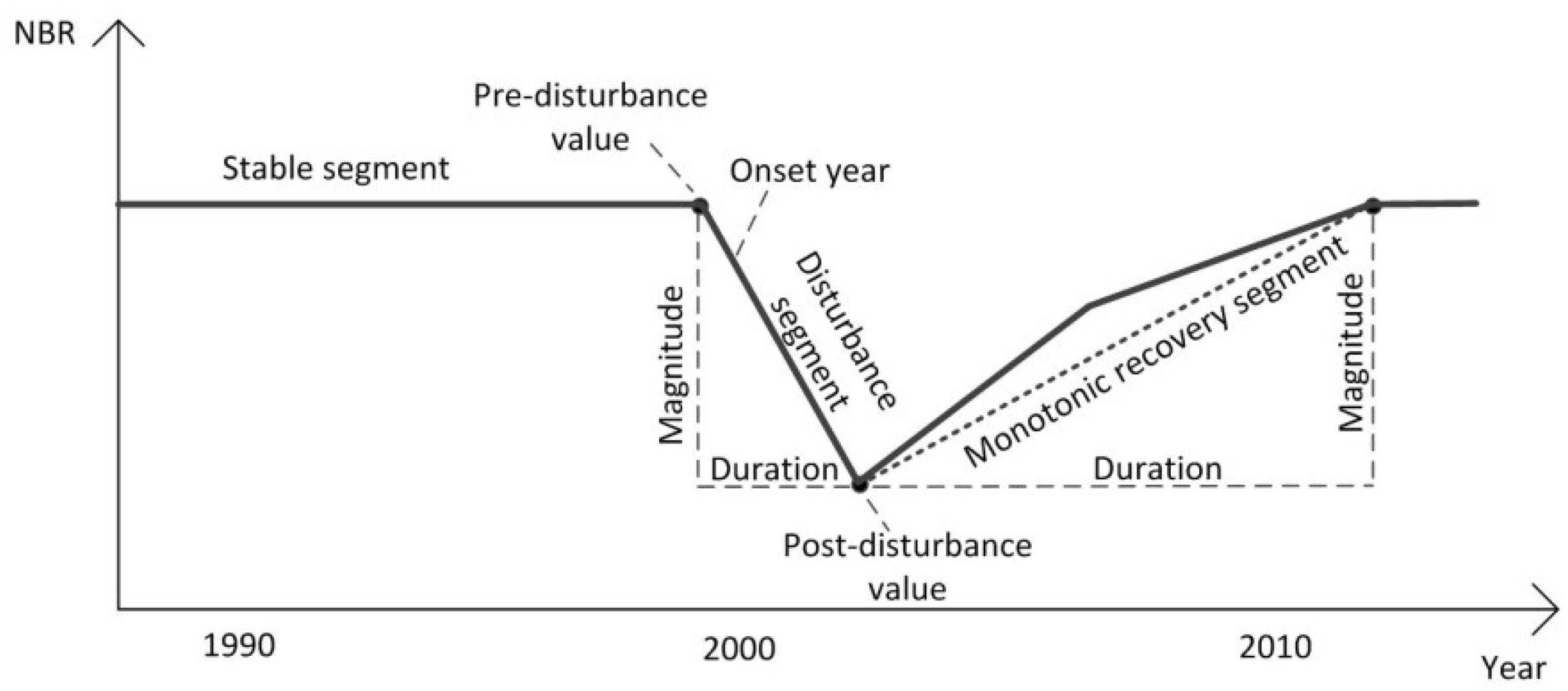
| Change metrics | Pre-disturbance value | NBR value at the start vertex of disturbance segment |
| Post-disturbance value | NBR value at the end vertex of disturbance segment | |
| Disturbance onset year | The year when disturbance begins | |
| Disturbance duration | Number of years between the start vertex and the end vertex of disturbance segment | |
| Disturbance magnitude | Difference in NBR value between the start vertex and the end vertex of disturbance segment | |
| Relative disturbance magnitude | Ratio of disturbance magnitude to pre-disturbance value | |
| Disturbance rate | Ratio of disturbance magnitude to disturbance duration | |
| Recovery onset year | The year when post-disturbance recovery starts | |
| Recovery duration | Number of years between the start vertex and the end vertex of recovery segment | |
| Recovery magnitude | Difference in NBR value between the start vertex and the end vertex of recovery segment | |
| Relative recovery magnitude | Ratio of recovery magnitude to post-disturbance value | |
| Recovery rate | Ratio of recovery magnitude to recovery duration | |
| Time since disturbance | Number of years since disturbance ends | |
| Disturbance level | High, medium, or low disturbance | |
| Disturbance causal agent | Fire, logging, and other (drought, insects, flood) | |
| Topographic and climatic metrics | Elevation | Elevation in meters |
| Slope | Slope in degrees | |
| Precipitation | Mean total rainfall | |
| Temperature | Mean annual temperature | |
| Location | X | Northing |
| Y | Easting |
| Response Variables | Model Scenarios | |||||
|---|---|---|---|---|---|---|
| BM | BA | TD | VL | BA-TD | VL-TD | |
| Biomass variables | ||||||
| AGBtotal | X | |||||
| AGBlive_tree | X | |||||
| AGBdead_tree | X | |||||
| Structure variables | ||||||
| BAlive_tree | X | X | ||||
| BAdead_tree | X | X | ||||
| TDlive_tree | X | X | ||||
| TDdead_tree | X | X | ||||
| VLlive_tree | X | X | X | |||
| VLdead_tree | X | X | X | |||
© 2018 by the authors. Licensee MDPI, Basel, Switzerland. This article is an open access article distributed under the terms and conditions of the Creative Commons Attribution (CC BY) license (http://creativecommons.org/licenses/by/4.0/).
Share and Cite
Nguyen, T.H.; Jones, S.; Soto-Berelov, M.; Haywood, A.; Hislop, S. A Comparison of Imputation Approaches for Estimating Forest Biomass Using Landsat Time-Series and Inventory Data. Remote Sens. 2018, 10, 1825. https://doi.org/10.3390/rs10111825
Nguyen TH, Jones S, Soto-Berelov M, Haywood A, Hislop S. A Comparison of Imputation Approaches for Estimating Forest Biomass Using Landsat Time-Series and Inventory Data. Remote Sensing. 2018; 10(11):1825. https://doi.org/10.3390/rs10111825
Chicago/Turabian StyleNguyen, Trung H., Simon Jones, Mariela Soto-Berelov, Andrew Haywood, and Samuel Hislop. 2018. "A Comparison of Imputation Approaches for Estimating Forest Biomass Using Landsat Time-Series and Inventory Data" Remote Sensing 10, no. 11: 1825. https://doi.org/10.3390/rs10111825