Towards Estimating Land Evaporation at Field Scales Using GLEAM
by
 , ,
, ,
Brecht Martens
1,* ,
,
Richard A. M. De Jeu
2,
Niko E. C. Verhoest
1,
Hanneke Schuurmans
3,
Jonne Kleijer
3 and
Diego G. Miralles
1 1
Laboratory of Hydrology and Water Management—Ghent University; Coupure links 653, 9000 Gent, Belgium
2
VanderSat BVBA, Wilhelminastraat 43a, 2011 VK Haarlem, The Netherlands
3
Royal HaskoningDHV, Laan 1914 35, 3818 EX Amersfoort, The Netherlands
*
Author to whom correspondence should be addressed.
Remote Sens. 2018, 10(11), 1720; https://doi.org/10.3390/rs10111720
Submission received: 27 September 2018
/
Revised: 24 October 2018
/
Accepted: 29 October 2018
/
Published: 31 October 2018
(This article belongs to the Special Issue Advances in the Remote Sensing of Terrestrial Evaporation)
Abstract
:The evaporation of water from land into the atmosphere is a key component of the hydrological cycle. Accurate estimates of this flux are essential for proper water management and irrigation scheduling. However, continuous and qualitative information on land evaporation is currently not available at the required spatio-temporal scales for agricultural applications and regional-scale water management. Here, we apply the Global Land Evaporation Amsterdam Model (GLEAM) at 100 m spatial resolution and daily time steps to provide estimates of land evaporation over The Netherlands, Flanders, and western Germany for the period 2013–2017. By making extensive use of microwave-based geophysical observations, we are able to provide data under all weather conditions. The soil moisture estimates from GLEAM at high resolution compare well with in situ measurements of surface soil moisture, resulting in a median temporal correlation coefficient of 0.76 across 29 sites. Estimates of terrestrial evaporation are also evaluated using in situ eddy-covariance measurements from five sites, and compared to estimates from the coarse-scale GLEAM v3.2b, land evaporation from the Satellite Application Facility on Land Surface Analysis (LSA-SAF), and reference grass evaporation based on Makkink’s equation. All datasets compare similarly with in situ measurements and differences in the temporal statistics are small, with correlation coefficients against in situ data ranging from 0.65 to 0.95, depending on the site. Evaporation estimates from GLEAM-HR are typically bounded by the high values of the Makkink evaporation and the low values from LSA-SAF. While GLEAM-HR and LSA-SAF show the highest spatial detail, their geographical patterns diverge strongly due to differences in model assumptions, model parameterizations, and forcing data. The separate consideration of rainfall interception loss by tall vegetation in GLEAM-HR is a key cause of this divergence: while LSA-SAF reports maximum annual evaporation volumes in the Green Heart of The Netherlands, an area dominated by shrubs and grasses, GLEAM-HR shows its maximum in the national parks of the Veluwe and Heuvelrug, both densely-forested regions where rainfall interception loss is a dominant process. The pioneering dataset presented here is unique in that it provides observational-based estimates at high resolution under all weather conditions, and represents a viable alternative to traditional visible and infrared models to retrieve evaporation at field scales.
1. Introduction
Terrestrial evaporation—the total flux of water from land to atmosphere—regulates continental water budgets, and is an essential variable for water resource management. It is also tightly linked to the process of photosynthesis, thereby connecting the hydrological and carbon cycles [1,2]. The consumption of energy during the evaporation process also controls the partitioning of energy at the surface, and ultimately the moisture content in the atmospheric boundary layer. As such, evaporation affects local and remote cloud formation, precipitation and air temperature [3,4,5,6]. This feedback can be critical for drought and heatwave occurrence and evolution, especially in regions and times where convection plays a dominant roll in the development of rainfall events [7,8]. Following the expected intensification and increasing frequency of droughts and heatwaves under future climate [9,10], the ability to mitigate the impacts of these events on our water resources, natural ecosystems, and food production systems strongly relies on the capability to predict the dynamics of evaporation during these events. That would allow for prompt and effective management in order to reduce socio-economic and natural impacts of extreme climate events. In addition, near-real time monitoring of land evaporation might enable the early diagnosis of agricultural droughts [11,12].
The estimation and observation of land evaporation at different spatio-temporal scales has achieved much attention in recent years [13,14,15,16,17,18,19]. Given the sparsity of in situ networks over land based on meteorological towers (e.g., eddy-covariance or Bowen-ratio), evaporation pans, or lysimeters, remote sensing has been put forward as alternative to routinely monitor evaporation and obtain spatially-distributed retrievals over large areas [20]. Because evaporation cannot be observed directly using remote sensors, different statistical or process-based models have been proposed to yield estimates of evaporation by combining remotely-observable variables related to this biophysical process [14,16,21]. However, datasets of land evaporation do not yet meet the requirements for local-scale water management and agricultural applications such as irrigation planning, which demand both high spatial (sub-kilometre) and temporal resolution (daily to sub-daily) [18].
Traditional methods typically use changes in land-surface temperature (LST), retrieved from remote sensors, to estimate terrestrial evaporation as a residual of the surface energy balance [22,23,24]. Nowadays, the use of LST—derived from thermal infrared (TIR) sensors onboard satellites [25], cubesats [26], or drones [27]—in these algorithms allows for estimating land evaporation at high spatial (up to 1 m using drones) and temporal resolutions (up to several minutes using geostationary imagery), with a limited need for ancillary data [25]. However, TIR measurements are affected by clouds [28], restricting the estimation of land evaporation to times with optimal weather conditions [29]. While estimates of LST from microwave (MW) observations might overcome this problem [28,30], they suffer from a substantially coarser native spatial resolution (several kilometres). In addition to these issues, energy-balance methods often target the accurate estimation of the sensible heat flux, relying on assumptions regarding the vertical temperature gradient and the aerodynamic conductance of the atmosphere, and calculate the evaporative flux as the residual of the surface energy balance [22,23,24,31].
Alternative methods to derive terrestrial evaporation directly target the flux using process-based algorithms. However, most of them have been originally designed for global-scale applications [32,33,34,35,36]. The Global Land Evaporation Amsterdam Model (GLEAM) is such a model, designed to estimate land evaporation and its separate components (i.e., transpiration, bare soil evaporation, rainfall interception loss, open-water evaporation, and sublimation) at the global scale using only remote sensing observations, primarily retrieved from MW sensors on polar-orbiting satellites [35]. Global datasets of terrestrial evaporation and root-zone soil moisture derived using GLEAM (www.gleam.eu) have been widely used to study the global water cycle [37,38] and land-atmosphere feedbacks [39,40] and to evaluate and improve land-surface models [41] and reanalysis datasets [42]. However, the application of GLEAM for local water management or agricultural planning has been hindered by its spatial resolution, resulting from the coarse-scale inputs typically used to force the model. Nonetheless, the algorithm is in principle applicable at finer resolutions if the required forcing data are available.
Recent progress in the field of Earth observation has resulted in a plethora of satellite-based observations spanning multiple spatial and temporal scales [19]. Also in the MW domain, efforts to combine measurements from different sensors and to improve retrieval algorithms [43,44,45] have resulted in the availability of MW-based geophysical parameters at field scales [45]. These advances enable the estimation of land evaporation using GLEAM at similar spatial scales.
Here, we force GLEAM using novel, all-weather, high-resolution (100 m) MW data over The Netherlands, Flanders and western Germany and assess the capability of the model to estimate land evaporation at these scales. We validate the high-resolution estimates of land evaporation against in situ measurements from five eddy-covariance towers within the study domain. In addition, we also evaluate the surface soil moisture estimates from GLEAM using in situ measurements from 29 soil moisture sensors. The quality of the high-resolution land evaporation dataset is further compared to similar datasets available over the study domain. Finally, we evaluate the spatial patterns of land evaporation, and discuss the response of evaporation to the summer drought in 2013. As GLEAM has been designed to estimate land evaporation at the global scale and relatively coarse spatial resolution (±25 km), this study will provide insights on the applicability of the model assumptions and structure at much finer resolution, which will foster the estimation of terrestrial evaporation at resolutions useful for local water management and agriculture.
2. Materials and Methods
2.1. GLEAM
GLEAM is a process-based semi-empirical model aiming at the estimation of land evaporation and its separate components [35]. Here, we employ the recently developed version 3 of the model [46]. The key aspects of GLEAM are (1) the extensive use of MW observations, enabling the estimation of land evaporation under cloudy conditions; (2) the detailed modelling of rainfall interception loss using the Gash analytical model [47,48,49]; and (3) the consideration of soil moisture and vegetation water content to constrain the estimates of potential evaporation.
The model first calculates potential evaporation using the Priestley and Taylor equation [50] for four sub-pixel land cover fractions: (1) open water; (2) low vegetation; (3) tall vegetation; and (4) bare soil. The Priestley and Taylor equation calculates potential evaporation by scaling the radiation-based term of the Penman–Monteith equation using the Priestley and Taylor constant, thereby only relying on net radiation and air temperature as inputs, thus avoiding the need for atmospheric humidity and near-surface winds, that are hard to observe from space. For the vegetated fraction, potential transpiration is constrained using a multiplicative evaporative stress factor based on root-zone soil moisture and MW vegetation optical depth (VOD) [46], a parameter closely linked to vegetation water content [51]. The root-zone soil moisture is calculated using a multi-layer water-balance model forced with observations of precipitation, and optimized via data assimilation of surface soil moisture. The data assimilation system is based on a Newtonian Nudging scheme, where the MW observations and modelled surface soil moisture are weighted based on their random errors, estimated using a triple collocation analysis [46,52]. The stress factor for the bare soil fraction is a function of surface soil moisture only, while for the fraction of open water no evaporative stress is assumed. For snow-covered pixels, sublimation is calculated using a specific parameterization of the Priestley and Taylor equation [53]. Rainfall interception loss is estimated for tall vegetation using the implementation of Gash’s analytical model of rainfall interception loss [47] by Valente et al. [48]. The latter is based on a water-balance model of the canopy forced with observations of precipitation, and taking into account both vegetation and rainfall properties. The total terrestrial evaporation results from the addition of transpiration, rainfall interception loss, bare soil evaporation, open-water evaporation and snow sublimation. For a detailed description of the model baseline, we refer to Miralles et al. [35,49] and Martens et al. [46,52].
2.2. Forcing Data
Table 1 lists the forcing datasets used in this study. All variables are processed over The Netherlands, Flanders and western Germany and are linearly resampled to a 100 m spatial grid and (when necessary) aggregated to a daily temporal resolution. The period considered is 2012–2017, yet 2012 is used as a spin-up for GLEAM [46], hence it will not be considered in the evaluation of the model. Except for the soil properties (used to parameterize the soil–water balance model in GLEAM), and the precipitation dataset, all forcing variables are obtained from satellite-based measurements. Note that atmospheric forcing variables (such as incoming radiation and precipitation) come originally at coarser spatial resolution, but because atmospheric forcing is more spatially uniform than the (heterogeneous) land properties, the use of 100 m as target resolution appears justified.
Aiming at the most accurate calculation of the available energy at the surface, radiation components from different satellite-based datasets are combined. Incoming shortwave () and longwave () surface radiation fluxes are retrieved from measurements of the Spinning Enhanced Visible and Infrared Imager (SEVIRI) onboard the Meteosat Second Generation (MSG) satellite, and are obtained from the EUMETSAT Satellite Application Facility on Land Surface Analysis (LSA-SAF, http://lsa-saf.eumetsat.int) [54]. The native spatial resolution of the SEVIRI instrument is 3.1 km at the nadir, but reduces towards approximately 5 km over Europe. Albedo—required to estimate the reflected shortwave radiation () at the surface—is sourced from measurements of the MODerate resolution Imaging Spectroradiometer (MODIS) instruments onboard Terra and Aqua. Here, the 16-day MCD43A3 albedo product [55] at 500 m spatial resolution is used, which is linearly resampled to a daily time interval. Finally, the emitted longwave radiation flux at the surface () is estimated using land-surface emissivity from LSA-SAF [54] and MW-based estimates of LST at 100 m spatial resolution from VanderSat (https://www.vandersat.com/) [45]. To obtain consistent radiation fluxes, each flux is individually scaled towards coarse-scale products obtained from measurements of the Clouds and the Earth’s Radiant Energy System (CERES) onboard Terra [56]. The scaling involves a multiplicative bias-correction at the 1° spatial resolution of CERES, preserving the higher resolution spatial features of the underlying datasets (Appendix A).
Precipitation is obtained from a network of five ground-based, C-band Doppler radars located in The Netherlands (operated by the Royal Meteorological Institute of The Netherlands, KNMI) and Germany (operated by the German Weather Service). Individual radar images are first merged, and subsequently corrected using in situ rain gauge measurements [57]. The final daily dataset is curated by Royal Haskoning DHV (https://www.royalhaskoningdhv.com/) and is available at a 1 km spatial resolution.
VOD, surface soil moisture, and LST are retrieved by the Land Parameter Retrieval Model (LPRM) [43,44,58] on downscaled measurements of the Advanced Microwave Scanning Radiometer 2 (AMSR-2) instrument onboard the GCOM-W1 satellite. The data are available at a daily time interval and 100 m spatial resolution [45]. Because GLEAM uses triple collocation to compute the uncertainties in the MW-based soil moisture that is assimilated [46,52], a third independent dataset of soil moisture is also required. Here, the soil–water index calculated from measurements of the Advanced Scatterometer (ASCAT) onboard Metop A and B from Albergel et al. [59] is adopted. Note that given the daily availability of MW surface soil moisture observations in this study, the nudging factor in the data assimilation system is decreased from the value of 1 proposed by Martens et al. [46,52] to a value of 0.25. The latter avoids that the model is nudged too strongly towards the observations and thus relaxes the dependence of the model estimates on the MW observations of surface soil moisture [60].
Next to the dynamic input discussed above, GLEAM also adopts three static datasets to describe the soil properties, spatial vegetation variability, and rainfall characteristics. Soil properties are obtained from the SoilGrids250m dataset [61] and land cover fractions from the MODIS MOD44B product [62], both available at 250 m resolution. The latter is a yearly product but is averaged over the study period to obtain a static map of vegetation fractions, as in Martens et al. [46]. Finally, similar to Miralles et al. [49], monthly average rainfall intensities used to model rainfall interception loss in GLEAM are obtained from the Combined Global Lightning Flash Rate Density monthly product [63] available at 5 km spatial resolution.
2.3. Evaluation Data
2.3.1. In Situ Soil Moisture and Evaporation
Table 2 shows the locations and data availability of the in situ eddy-covariance measurements. Note that in situ measurements are only processed for the period 2013–2017, as 2012 is used to spin up GLEAM (Section 2.2). Measurements from NL-Ca1 are downloaded from the Cabauw Experimental Site for Atmospheric Research (CESAR) web portal, while data from DE-RuR originates from the TERENO data infrastructure. Data from DE-RuS is sourced from the European Fluxes database cluster, and measurements from BE-Bra and NL-Loo are acquired from the FLUXNET 2015 dataset. All eddy-covariance datasets are processed as in Martens et al. [46], including (1) masking of unreliable data based on quality flags in the official datasets; (2) masking of outliers and repetitive measurements; (3) masking of rain intervals—identified using precipitation data included in the dataset, and the precipitation forcing (Table 1)—to avoid the use of unreliable measurements from wet sensors [64]; and (4) aggregation to a daily temporal resolution.
In situ measurements of surface soil moisture (i.e., sensors installed at a maximum depth of 10 cm, corresponding to the lower level of the first soil layer in GLEAM) are obtained from the database of the International Soil Moisture Network (ISMN) [65,66], and the regional soil moisture network in the Raam catchment [67]. Data are processed using a similar procedure as for the eddy-covariance data, except for the rain mask, which is not applied.
Aiming at a robust validation, only stations reporting a minimum of 150 measurements after masking are considered in this study, resulting in a validation dataset with measurements from five eddy-covariance towers (Table 2), and 29 surface soil moisture sensors. Note that measurements from sensors falling within the same 100 m model pixel are not averaged to avoid potential problems with data gaps and biases between in situ sensors. Figure 1 shows the locations of the in situ sites within the bounding box of the study domain, with the multi-annual yearly normalized difference vegetation index from LandSat 8 as a background. Eddy-covariance sites span different vegetation types and are well-distributed across the study domain, as shown in Figure 1. Soil moisture validation sites, on the other hand, are clustered in the Eifel area in west Germany, and the Raam catchment in the east of The Netherlands. The latter is an intensively-measured, medium-scale 223 km2 catchment where data from 14 soil moisture sensors are available [67]. Also note that measurements of both surface soil moisture and evaporation are available at three sites (Table 2 and Figure 1).
2.3.2. Gridded Evaporation
The high-resolution GLEAM evaporation data (hereafter referred to as GLEAM-HR) are also compared against the LSA-SAF [54], GLEAM v3.2b [46], and Makkink (https://data.knmi.nl/) daily evaporation products.
LSA-SAF is obtained from forcing a physically-based soil vegetation atmosphere model with inputs derived from MSG-SEVIRI and meteorological forecasts from the European Centre for Medium-Range Weather Forecasts (ECMWF) [72]. Similar to GLEAM, the algorithm first estimates evaporation for several sub-pixel land-cover units—characterized using the ECOCLIMAP dataset [73]—and aggregates the resulting estimates to the pixel level. The model is parameterized using look-up tables and the ECOCLIMAP dataset. Estimates are available at the native resolution of the MSG-SEVIRI instrument, which is approximately 5 km over western Europe.
GLEAM v3.2b is a daily, global, satellite-based dataset of terrestrial evaporation, available at 0.25° spatial resolution [46]. It is based on the same version of the GLEAM model that is adopted here, but forced with coarse-resolution inputs.
Finally, KNMI provides a daily evaporation product for The Netherlands by interpolating reference grass evaporation estimated from meteorological measurements at 32 sites using the Makkink equation [74,75]. The latter is a radiation-based approach and only provides an estimate of land evaporation for a well-watered reference grass. The estimates are then interpolated using a thin plate spline method over a 10 km grid.
3. Results and Discussion
3.1. Temporal Evaluation of Surface Soil Moisture
Given the relatively high volumes of rainfall, water availability is generally not limiting the evaporative flux in the study domain [75,76,77]. Nevertheless, a validation of the soil moisture estimates from GLEAM-HR against in situ measurements serves the purpose of identifying potential issues with regards to the input data and tests the validity of the algorithm at high resolutions. Figure 2 shows violin plots of the validation statistics calculated at the 29 in situ sites with surface soil moisture measurements. Statistics are shown for the MW observations that are assimilated in GLEAM-HR (Table 1), GLEAM-HR without data assimilation (i.e., the open loop), GLEAM-HR with assimilation of MW soil moisture, and the coarse-scale GLEAM v3.2b.
Soil moisture estimates from GLEAM-HR compare reasonably well against in situ measurements, with a median correlation (R) of 0.76, and values below 0.64 at only seven of the in situ sites (Figure 2a). The estimates are close to unbiased (Figure 2b), but show a small tendency to overestimate the in situ data. Mean absolute differences (MAD) roughly vary between 0.03 and 0.13 m3·m−3 (95%-interval), with a median of 0.07 m3·m−3 (Figure 2c). Part of the latter value is attributed to the bias, as the unbiased MAD (ubMAD) has a median close to 0.04 m3·m−3 (Figure 2d), which is below the threshold of 0.05 m3·m−3 that is often considered as the target accuracy for satellite-based soil moisture datasets [78,79].
The MW soil moisture observations generally show lower correlations (median of 0.67, Figure 2a) than the open loop of GLEAM-HR, but comparable ubMAD (median of 0.04 m3·m−3, Figure 2d). In addition, the bias of the MW observations is close to zero, with a tendency to underestimate the in situ soil moisture (Figure 2b). Assimilating the MW observations in GLEAM-HR has a small but positive impact on the estimates of surface soil moisture: comparing the violin plots of GLEAM-HR against the ones for the open loop of GLEAM-HR reveals an overall increase in R (upward shift of the distribution, Figure 2a). Note that the MD of the open loop and GLEAM-HR are the same (Figure 2b), as the data assimilation includes a scaling of the MW observations towards the soil moisture estimates of the open loop [46,52]. The impact of the data assimilation system on the MAD and ubMAD is less clear, but slightly positive (Figure 2c,d). The relatively simple data assimilation algorithm implemented in GLEAM-HR is thus able to extract valuable information from the MW observations, and to increase the overall quality of the GLEAM-HR soil moisture estimates.
Temporal statistics in Figure 2 reveal that the soil moisture dynamics from the global GLEAM v3.2b are equally reliable, despite their coarser spatial resolution. Figure 2a shows that both the median and third quartile of the R-distribution are rather similar for GLEAM-HR and GLEAM v3.2b. However, the correlation coefficient at a couple of sites is lower for GLEAM-HR, while, for GLEAM v3.2b, the correlation coefficients are consistently concentrated around their median value of 0.78. The bias (Figure 2b) of GLEAM-HR, on the other hand, is considerably lower, also resulting in lower values of the MAD (Figure 2c), while the ubMAD is similar for both datasets (Figure 2d). The lower bias for GLEAM-HR can be attributed to the added realism of the soil properties used in GLEAM-HR that set the range of absolute soil moisture values. Differences in R and the ubMAD, on the other hand, reflect discrepancies in the dynamic forcing used in both. Uncertainties in net radiation and, to the largest extent, precipitation control the temporal variability of the surface soil moisture estimates from GLEAM-HR and its agreement against in situ measurements.
Although the ground-based radar composite used in this study (Table 1) covers western Germany and Flanders, the quality over these regions is lower due to the lower number of in situ rain gauges in these areas available to correct the radar retrievals (note that this effect might also occur along the coast of The Netherlands, since only inland gauges are used here) [57]. Only considering soil moisture validation sites in The Netherlands has a clear and positive impact on the validation statistics of GLEAM-HR (Figure A1), as most sites with poor validation statistics are removed from the sample. In addition, both the median and third quartile of the R-distribution are higher than the ones from GLEAM v3.2b at the same sample of sites, while the first quartile of the distribution still remains slightly lower (Figure A1a). Conclusions in terms of MD, MAD, and ubMAD remain similar (Figure A1b–d).
We would like to emphasize that the results for this evaluation may not provide an unbiased assessment of the quality of soil moisture over the entire domain, due to the high concentration of in situ sensors in the Raam catchment (Figure 1), while only a limited number of sensors is available in other parts of the study area with different soil properties, land cover, and atmospheric forcing. Given the strong spatial variability of parameters dominating the temporal dynamics (and spatial patterns) of surface soil moisture, it is thus difficult to generalize our results to the whole study area.
3.2. Evaluation of Evaporation
3.2.1. Temporal Evaluation
Figure 3 shows the validation statistics for the estimates of land evaporation from GLEAM-HR, the open loop of GLEAM-HR, GLEAM v3.2b, LSA-SAF, and the Makkink dataset at each eddy-covariance site. Estimates from GLEAM-HR compare well with in situ measurements of evaporation, with a median correlation coefficient of 0.78 across all five sites. On average, a slight negative bias is observed, except for BE-Bra and NL-Loo, where GLEAM-HR tends to overestimate evaporation. The ubMAD ranges between 0.37 mm·day−1 at NL-Ca1 and 0.77 mm·day−1 at NL-Loo.
The impact of soil moisture data assimilation on the estimates of evaporation from GLEAM-HR is negligible due to the relatively wet climate in the study domain, and consequently, the low control of soil–water availability on land evaporation [75,76,77]. Averaged over the five eddy-covariance sites, surface soil moisture from GLEAM-HR only drops below the critical soil moisture—i.e., the value where evaporation starts to be limited by soil–water availability—at 11% of the days in the study period.
In general, inter-dataset differences in temporal validation statistics are low. GLEAM v3.2b shows slightly higher values for R at BE-Bra and NL-Loo, but worse ubMAD at DE-Rur and NL-Ca1 as compared to GLEAM-HR. LSA-SAF is the only dataset consistently underestimating the in situ measurements, but shows similar values for the other statistics.
On the other hand, validation statistics differ substantially between the five in situ sites. At DE-Rur, DE-Rus, and NL-Ca1, all products perform considerably better than at the other two sites, with correlation coefficients reaching 0.9 at the sites in Germany, and 0.95 at NL-Ca1, indicative of the strong temporal agreement between the products and the in situ measurements. Similar conclusions may be drawn for the other statistics, except at DE-RuS, where the bias and MAD are also the highest across all sites, and for all products. At BE-Bra and NL-Loo, all products perform relatively worse, with values for R between 0.6 and 0.7, depending on the dataset and eddy-covariance site. Note that eddy-covariance measurements tend to underestimate the latent heat flux and that the energy balance is generally not closed due to sub-optimal atmospheric conditions for eddy-covariance calculations at certain times, mismatch in the spatial footprint of different sensors at the tower, and poor characterization of the soil heat flux [80,81]. As such, the consistently worse performance by all models at certain sites might reflect uncertainty in the in situ data as well. In the case of BE-Bra, the site is in the close proximity of an urban area; the impact of this aspect on the measurements, and the fact that none of the algorithms considered here parameterizes specifically urban areas, may affect validation results as well.
At NL-Ca1 and NL-Loo, we also evaluate the Makkink dataset (note that the Makkink dataset is only available over The Netherlands; see also Section 2.3.2). Correlation coefficients of 0.95 and 0.6 are obtained for NL-Ca1 and NL-Loo, respectively, similar to the other datasets. However, the dataset consistently overestimates land evaporation at both sites, as the Makkink equation only considers the atmospheric demand for water over a reference grass, and does not account for any land surface control over the flux. The high correlation indicates the strong temporal agreement between potential and actual evaporation over The Netherlands, which has already been highlighted by Jacobs and De Bruin [76] and Jacobs et al. [77]. The bias, on the other hand, demonstrates the need for a proper (seasonally-dependent) crop coefficient to account for the land surface control over the flux.
Figure 4 shows time series of GLEAM-HR, GLEAM v3.2b, LSA-SAF, and the Makkink dataset at NL-Ca1 and NL-Loo. These time series show that all products are able to capture the seasonal cycle of land evaporation at both sites. As expected, differences at NL-Ca1 are small, and all products closely follow the in situ measurements. At NL-Loo, more explicit differences are found, especially during winter time where GLEAM-HR and GLEAM v3.2b show both larger variability and absolute values of evaporation. This might be explained by the explicit consideration of rainfall interception loss in the algorithm, which becomes relatively more important during winter given the low volumes of transpiration and bare soil evaporation. Note that this can also be seen at NL-Ca1, although less clear. Also in summer 2013, clear differences between the products can be found at NL-Loo, which can be related to the different sensitivities of the algorithms to decreasing soil–water availability (see also Section 3.3).
3.2.2. Spatial Evaluation
Figure 5 shows the multi-year (2013–2017) mean of annual evaporation from GLEAM-HR (a), GLEAM v3.2b (b), LSA-SAF (c), and the Makkink product (d), and the difference of each with the multi-product ensemble mean (e–h). Note that we limit the study area to The Netherlands here because of the lower quality of the radar rainfall in GLEAM-HR outside the country (Section 3.1), and the fact that the Makkink product is only available for this area. All datasets show substantial differences, with GLEAM-HR and GLEAM v3.2b typically bounded by the low values from LSA-SAF, and the high values from the Makkink dataset. The mean evaporation over The Netherlands amounts to 494, 569, 437, and 602 mm·year−1 for GLEAM-HR, GLEAM v3.2b, LSA-SAF, and the Makkink product, respectively. Note that the high values for the Makkink dataset are due to the fact that it represents reference grass evaporation rather than actual evaporation [74]. The lower values in LSA-SAF, on the other hand, might relate to the non-specific consideration of rainfall interception loss [72], which represents a substantial fraction of the total flux in forested areas [36,82].
Despite similar temporal statistics (Section 3.2.1), all datasets show substantially different spatial patterns. The highest spatial detail is reflected by GLEAM-HR (Figure 5a). On the other hand, the Makkink dataset shows a smooth spatial pattern due to its spline interpolation based on a limited number of stations (Section 2.3.2), and its high dependency on total incoming radiation [74], which reflects a very gradual increase towards the southwest (Figure 5d). However, spatial gradients in the Makkink dataset are small as compared to the other datasets (note the different colour range in Figure 5a–d).
Although obtained using the same algorithm, GLEAM v3.2b and GLEAM-HR show substantial differences in their spatial detail and magnitudes. Obviously, the higher spatial detail in GLEAM-HR can be attributed to the high-resolution forcing and more detailed parameterization of the land surface. Given that the radiation forcing of GLEAM-HR is bias-corrected using the GLEAM v3.2b radiation forcing (see Section 2.2), differences in magnitude are most probably due to the rainfall forcing, mainly affecting the interception loss volume in the study domain. Note that, given the low evaporative stress throughout the year, the effect of the rainfall forcing on the other evaporation components is negligible.
The overall patterns in GLEAM-HR and LSA-SAF are substantially different as well (Figure 5a,c). Both datasets agree on the lower values near the coast, which relate to the presence of large urban areas like Rotterdam, the Hague, and Amsterdam (Figure A2a). While urban areas are not explicitly modelled in any of the algorithms, they are associated with a large fraction of bare soil and high land surface temperatures, which yields low evaporation estimates. In case of LSA-SAF, the low values for most cities in The Netherlands (Figure A2a) are more apparent (Figure 5c). The maximum annual evaporation is reported by LSA-SAF at approximately 52°N–5°E in the Green Heart of The Netherlands, a large vegetated area dominated by low vegetation types such as shrubs and grasses (Figure A2a). While GLEAM-HR shows similar values of approximately 500 mm·year−1 in this region, its two spatial maxima occur eastwards, in the national parks of Heuvelrug (52.25°N–5.25°E) and the Veluwe (52.25°N–5.75°E), both densely-forested regions (Figure A2a). The dense vegetation together with the high precipitation volumes in the region [83] result in large fluxes of transpiration and rainfall interception loss. This effect is also apparent in smaller forested areas in the south and east of The Netherlands (Figure A2a and Figure 5a). Note that this pattern is not captured by LSA-SAF, as rainfall interception loss is not explicitly modelled, plus it occurs during cloudy periods when retrievals from Meteosat are either not available or of lower quality.
3.3. Summer Drought 2013
In 2013, only 740 mm of precipitation was recorded over The Netherlands, approximately 100 mm less than the long-term multi-annual average (https://www.knmi.nl/). The year 2013 can thus be considered as a relatively dry year, with below-average precipitation during January–April and June–August. As discussed in Section 3.2.1, soil–water availability is generally not affecting the evaporation rate in The Netherlands. Hence, potential evaporation is maintained for large parts of the year; i.e., the surface is able to supply the atmospheric demand for water [75,76,77]. However, during dry spells, soil water can be exceptionally low, resulting in evaporative water stress and a consequent reduction in land evaporation. In addition, below-average rainfall also results in reductions of rainfall interception loss, which substantially affect the total evaporative flux in forested regions.
Figure 6a shows the anomaly of the cumulative evaporation curve for 2013 (averaged over The Netherlands), relative to the multi-annual (2013–2017) mean for GLEAM-HR, LSA-SAF, and the Makkink dataset. The annual volume of evaporation in 2013 is approximately 20 mm (−4.5%, LSA-SAF), 25 mm (−4%, Makkink), and 28 mm (−5.5%, GLEAM-HR) less than the the climatological mean of each product. While these volumes are relatively similar, each dataset shows substantially different temporal dynamics in the anomaly time series, especially during summer (Figure 6a), when evaporation volumes are higher and the rainfall anomaly is stronger. The Makkink dataset shows a decrease in the curve at the beginning of summer, but an increase from July onward, following the dynamics of surface net radiation (Figure 7a). LSA-SAF, on the other hand, shows a relatively horizontal curve during summer, indicating that—averaged over The Netherlands—evaporation is close to normal during this period. Finally, GLEAM-HR shows a decreasing trend in the curve during all summer months, with the steepest decrease in August–September, coinciding with the strongest anomaly in precipitation (Figure 7a).
Figure 6b–j reveal that the spatial response of land evaporation to the 2013 summer drought also differs substantially per product. As expected, the Makkink dataset does not respond to the drought in 2013 and fully follows the radiation patterns (Figure 7e–g), resulting in below-average evaporation in June (Figure 6h), and above-average evaporation in July–August (Figure 6i,j). LSA-SAF and GLEAM-HR both consider a soil–water constraint on evaporation, and do respond to the rainfall deficits. However, the spatial patterns of the evaporation anomalies in both datasets are substantially different, with, in general, a more conservative response of LSA-SAF (compared to GLEAM-HR) to the rainfall anomalies. Note that the patterns in LSA-SAF can generally not be related to the precipitation and radiation anomalies shown in Figure 7, suggesting that other variables used to force the algorithm are responsible for driving the patterns.
Evaporation anomalies from GLEAM-HR (Figure 6b–d) during the summer drought mainly follow the anomalies in the estimated soil moisture from GLEAM-HR (Figure A3), which are strongly affected by the rainfall patterns (Figure 7b–d). As shown, negative anomalies in evaporation as a result of water stress first develop in sandy soils (Figure A2b), characteristic of their low water holding capacity. This effect can clearly be observed in August, when the cumulative rainfall deficit almost reaches its maximum (Figure 7a): while root-zone soil moisture anomalies are negative throughout the country, the strongest evaporation anomalies are found in sandy soils, while anomalies in clayey soils more towards the west are positive (Figure A2b). The latter is explained by the larger water holding capacity of these soils. Although the root-zone soil moisture is strongly depleted and anomalously low, soil water is still available to (partly) meet the atmospheric demand for water set by the positive anomaly in net radiation (Figure 7g).
The different response of LSA-SAF and GLEAM-HR to rainfall deficits can be explained by differences in the parameterization of soil moisture stress. While GLEAM-HR adopts a relatively simple (nonlinear) stress curve [46], LSA-SAF uses the more complex—yet still empirical—Jarvis function to calculate stomatal conductance and to convert potential into actual evaporation [72,84]. In addition, differences in forcing and forcing uncertainty affect the response of land evaporation to drought conditions. In GLEAM-HR, root-zone soil moisture is internally calculated using a simple water-balance model, forced by high-resolution observations of precipitation, and updated using a soil moisture data assimilation system. In LSA-SAF, on the other hand, root-zone soil moisture is obtained from the ECMWF operational forecast model which provides data at coarser spatial resolution than the target resolution of LSA-SAF [72]. Given the high spatial variability of root-zone soil moisture as a result of the heterogeneity in soil properties, vegetation cover, and (to a lesser extent) atmospheric forcing, the coarse-scale soil moisture in LSA-SAF thus underestimates this variability and its impact on evaporation. In addition, note that, in addition to the differences in soil moisture stress resulting in reduced transpiration and soil evaporation, GLEAM-HR also considers rainfall interception loss, which strongly affects the total evaporation in densely-forested areas.
4. Conclusions
GLEAM is a relatively simple process-based model originally designed to estimate land evaporation for climatological studies, running at coarse resolution and global scales [35]. This study evaluated for the first time the potential of GLEAM to be applied at field scales. As such, the model was forced using all-weather, high-resolution inputs (100 m) over The Netherlands, Flanders and western Germany and the estimates of root-zone soil moisture and land evaporation from GLEAM-HR were evaluated against a sample of in situ measurements from soil moisture sensors (29 sites) and eddy-covariance towers (five sites). In addition, GLEAM-HR was compared against the coarse-scale GLEAM v3.2b product (±25 km), the LSA-SAF evaporation product (±5 km), and the Makkink evaporation product from KNMI (10 km). Spatial patterns were also inter-compared, and their ability to respond to water stress was evaluated during the summer drought in 2013.
The temporal evaluation of GLEAM-HR against in situ data showed the ability of the model to retrieve temporal dynamics of surface soil moisture, as indicated by a median R and ubMAD across all sensors of 0.76 and 0.04 m3·m−3, respectively. In addition, the relatively simple data assimilation system in GLEAM-HR was able to extract valuable information from the MW observations of soil moisture, yielding a mild improvement in the temporal dynamics. Meanwhile, the coarse-resolution GLEAM v3.2b showed equally realistic temporal dynamics in soil moisture, with even a slightly better performance than GLEAM-HR in regions outside the The Netherlands, where the quality of the ground-based radar rainfall product—used as an input in GLEAM-HR—is lower.
The estimates of land evaporation from GLEAM-HR were validated against measurements from five eddy-covariance sites, resulting in correlation coefficients ranging between 0.65 and 0.95, comparable to the statistics from GLEAM v3.2b, LSA-SAF, and the Makkink dataset from KNMI. Estimates from GLEAM-HR appeared bounded by the low values from LSA-SAF and the high values from the Makkink dataset. Despite the similar temporal validation statistics, an in-depth analysis of the spatial patterns in evaporation yielded remarkable differences across all four datasets. The Makkink product showed almost no spatial variability due to its smoothing spline interpolation of a short range of in situ estimates, and GLEAM v3.2b showed only little spatial detail as a result of its coarse resolution. Both LSA-SAF and GLEAM-HR, on the other hand, showed high spatial heterogeneity, but patterns were different due to diverging model parameterizations, model assumptions, and forcing data. The most prevalent difference was attributed to the detailed modelling of rainfall interception loss in GLEAM-HR, an important flux in forested regions which is not well captured in LSA-SAF. As a result, the annual maximum evaporation from GLEAM-HR occured in the national parks of the Veluwe and Heuvelrug, located in the center of The Netherlands, and both densely-forested regions. LSA-SAF, on the other hand, showed its maximum in the Green Heart of The Netherlands, a region dominated by lower vegetation types such as grasses and shrubs.
Finally, we evaluated the response of land evaporation to the 2013 summer drought in The Netherlands. While the Makkink product is only constrained by surface net radiation and does not respond to changes in precipitation, both LSA-SAF and GLEAM-HR showed below-average evaporative fluxes in the epicentre of the drought. However, the negative anomalies of GLEAM-HR were larger, presumably as a result of the higher sensitivity of land evaporation to root-zone soil moisture and differences in forcing data.
Overall, GLEAM-HR produced qualitative and spatially consistent estimates of root-zone soil moisture and land evaporation at spatial resolutions useful for agricultural and water management purposes. Because the algorithm is designed to rely (to a large extent) on MW-based datasets of environmental forcing variables, resulting in all-weather output, it has an indisputable advantage over more traditional approaches applied at regional scales based on optical and infrared data [22,23,24]. The reliance on a Priestley and Taylor framework makes it feasible to run on remote sensing observations only, and avoids the need for reanalysis data like other remote sensing models designed for the large scale monitoring of evaporation [18,21].
Nonetheless, the skill of GLEAM-HR to produce high-resolution land evaporation needs to be further evaluated. As our study domain is relatively uniform in terms of topography and atmospheric conditions, the performance of GLEAM-HR in other evaporation regimes—especially water-limited regions—needs to be further investigated. Moreover, although the spatial patterns produced by GLEAM-HR can be linked to specific landscape features, a formal spatial validation of the estimates was hampered by the limited number of in situ measurements across the study domain. A more in-depth evaluation is thus necessary in order to assess the ability of GLEAM-HR to estimate realistic spatial variability in land evaporation. Nevertheless, as a first attempt to apply GLEAM at high resolution, this study provided promising insights and demonstrated the potential of the algorithm for regional-scale applications.
Aiming at improving the applicability of GLEAM-HR, future efforts should focus on (1) enhancing the spatio-temporal characteristics of the observational forcing data; (2) further evaluating and improving the process-based algorithms to cope with potential issues arising from the increasing resolution; (3) incorporating explicitly processes such as irrigation or urban infrastructures that are relevant at the finer scales; and (4) reducing the latency time, aiming for an operational dataset that can be of use for decision-making in agricultural and water management applications.
5. Data Availability
The CERES radiation components can be obtained from https://ceres.larc.nasa.gov/. The Meteosat LSA-SAF data can be ordered at https://landsaf.ipma.pt/. The MODIS albedo and land cover fractions can be downloaded from https://lpdaac.usgs.gov/. The ASCAT soil–water index can be obtained from https://land.copernicus.eu/. VOD, LST, and surface soil moisture from VanderSat can be obtained upon request from Richard de Jeu. Precipitation from the weather radar network can be obtained upon request from Hanneke Schuurmans. The SoilGrids250m database can be downloaded from https://soilgrids.org/. The lightning frequency from LIS/OTD can be obtained from https://ghrc.nsstc.nasa.gov/home/. The Makkink dataset can be downloaded from https://data.knmi.nl/. In situ validation data can be obtained using the data portals listed in Section 2.3.1. The high-resolution evaporation and root-zone soil moisture datasets presented in this study can be obtained upon request from the corresponding author.
Author Contributions
Conceptualization, B.M., R.A.M.d.J. and D.G.M.; Data Curation, B.M., R.A.M.d.J., H.S. and J.K.; Formal Analysis, B.M.; Funding acquisition, R.A.M.d.J., H.S. and D.G.M.; Investigation, B.M.; Methodology, B.M. and D.G.M.; Project Administration, R.A.M.d.J. and D.G.M.; Software, B.M. and D.G.M.; Supervision, R.A.M.d.J. and D.G.M.; Validation, B.M. and D.G.M.; Visualization, B.M. and D.G.M.; Writing—Original Draft, B.M.; Writing—Review and Editing, B.M., R.A.M.d.J., N.E.C.V. and D.G.M.
Funding
This research was funded by the Dutch ministry of economic affairs grant number SBIRSATW14. The APC was funded by the Dutch ministry of economic affairs.
Acknowledgments
Part of this work is funded by the Dutch ministry of economic affairs through the Small Business Innovation Research (SBIR) program: Satellietdata gebruik bij de dagelijkse schatting van landsdekkende verdampingsinformatie op bewolkte dagen (GLEAM-HR) (Use of satellite-based datasets for estimating land evaporation at cloudy days); project SBIRSATW14. D.G.M. acknowledges support from the European Research Council (ERC) under grant agreement 715254 (DRY–2–DRY). The computational resources (Stevin Supercomputer Infrastructure) and services used in this work were provided by the VSC (Flemish Supercomputer Center), funded by Ghent University, FWO, and the Flemish Government—department EWI. The MODIS MCD43A3 and MOD44B data products were retrieved from the online Data Pool, courtesy of the NASA Land Processes Distributed Active Archive Center (LP DAAC), USGS/Earth Resources Observation and Science (EROS) Center, Sioux Falls, South Dakota (https://lpdaac.usgs.gov/data_access/data_pool). In situ measurements of surface soil moisture were sourced from the International Soil Moisture Network (ISMN), and the regional soil moisture network in the Raam catchment (https://doi.org/10.4121/uuid:dc364e97-d44a-403f-82a7-121902deeb56). Data from NL-Ca1 were downloaded from the Cabauw Experimental Site for Atmospheric Research (Cesar) web portal. Data from DE-RuR originates from the TERENO data infrastructure, which is made available under the ODC Attribution License. Data from DE-RuS and BE-Lon were downloaded from the European Fluxes database cluster. Data from BE-Bra and NL-Loo were acquired and shared by the FLUXNET community, including these networks: AmeriFlux, AfriFlux, AsiaFlux, CarboAfrica, CarboEuropeIP, CarboItaly, CarboMont, ChinaFlux, Fluxnet-Canada, GreenGrass, ICOS, KoFlux, LBA, NECC, OzFlux-TERN, TCOS-Siberia, and USCCC. The FLUXNET eddy covariance data processing and harmonization was carried out by the ICOS Ecosystem Thematic Center, AmeriFlux Management Project and Fluxdata project of FLUXNET, with the support of CDIAC, and the OzFlux, ChinaFlux and AsiaFlux offices.
Conflicts of Interest
The authors declare no conflict of interest.
Appendix A. Bias-Correction Radiation Components
The fine-scale surface radiation components (, , , )—estimated from several inconsistent data sources (Table 1)—are individually scaled towards coarse-scale measurements from CERES [56] to obtain consistent fluxes. The scaling involves a multiplicative bias correction of the fine-scale fluxes towards CERES, preserving the spatial detail, but removing the absolute mismatch between the two at the coarse scale.
First, the coarse-scale field is interpolated over the fine-scale grid using a nearest neighbour interpolation. For each fine-scale pixel (), a multiplicative bias correction factor is then calculated by convolving the ratio of the fine (F) and coarse-scale field (C), with a Gaussian kernel of one-sided width w (). The bias-corrected fine-scale field () can then be calculated as:
Equation (A1) can also be written as:
Equation (A2) shows that the bias-correction factor for pixel in the fine-scale grid is essentially a weighted average of the multiplicative correction factors within a neighbourhood of that pixel. The actual size of the neighbourhood w equals ± 50 km, approximately half of the resolution of CERES. Weights within the neighbourhood vary according to a Guassian function with standard deviation equal to one fourth of w, meaning that weights drop rapidly with the distance from pixel , and approach essentially zero for distances >25 km from .
Appendix B. Supplementary Figures
Figure A1.
Violin plots of the validation statistics of surface soil moisture from microwave observations (MW-OBS), GLEAM-HR without data assimilation (OL), GLEAM-HR, and GLEAM v3.2b. Violins represent the distribution of the validation statistics with indication of the median (white dot), interquartile range (thick line), and 95% interval (thin line). Individual statistics are calculated for 17 soil moisture sensors in The Netherlands and include (a) Pearson correlation coefficient (R); (b) mean difference (MD, in situ as a reference); (c) mean absolute difference (MAD); and (d) unbiased MAD (ubMAD).

Figure A2.
(a) Land cover obtained from the global European Space Agency Climate Change Initiative land cover classification map (2015), and (b) simplified soil map of The Netherlands from the Wageningen University and Research, Environmental Research group (Alterra) [85]; (b) “S.”, “Cl.”, “L”, and “H” refer to “Sandy”, “Clayey”, “Light”, and “Heavy”, respectively.

Figure A3.
Anomalies of soil moisture from GLEAM-HR in 2013. Maps show monthly anomalies of surface soil moisture (SSM), (a–c), and root-zone soil moisture (RZSM), (d–f) from GLEAM-HR (m3·m−3). Anomalies are calculated relative to the multi-annual (2013–2017) average monthly values.
Figure A3.
Anomalies of soil moisture from GLEAM-HR in 2013. Maps show monthly anomalies of surface soil moisture (SSM), (a–c), and root-zone soil moisture (RZSM), (d–f) from GLEAM-HR (m3·m−3). Anomalies are calculated relative to the multi-annual (2013–2017) average monthly values.

References
- Le Quéré, C.; Andrew, R.M.; Canadell, J.G.; Sitch, S.; Ivar Korsbakken, J.; Peters, G.P.; Manning, A.C.; Boden, T.A.; Tans, P.P.; Houghton, R.A.; et al. Global carbon budget 2016. Earth Syst. Sci. Data 2016, 8, 605–649. [Google Scholar] [CrossRef]
- Cheng, L.; Zhang, L.; Wang, Y.P.; Canadell, J.G.; Chiew, F.H.S.; Beringer, J.; Li, L.; Miralles, D.G.; Piao, S.; Zhang, Y. Recent increases in terrestrial carbon uptake at little cost to the water cycle. Nat. Commun. 2017, 8, 110. [Google Scholar] [CrossRef] [PubMed] [Green Version]
- Seneviratne, S.I.; Corti, T.; Davin, E.L.; Hirschi, M.; Jaeger, E.B.; Lehner, I.; Orlowsky, B.; Teuling, A.J. Investigating soil moisture-climate interactions in a changing climate: A review. Earth-Sci. Rev. 2010, 99, 125–161. [Google Scholar] [CrossRef]
- Taylor, C.M.; de Jeu, R.; Guichard, F.; Harris, P.P.; Dorigo, W.A. Afternoon rain more likely over drier soils. Nature 2012, 489, 423–426. [Google Scholar] [CrossRef] [PubMed] [Green Version]
- Teuling, A.J.; Taylor, C.M.; Meirink, J.F.; Melsen, L.A.; Miralles, D.G.; van Heerwaarden, C.C.; Vautard, R.; Stegehuis, A.I.; Nabuurs, G.J.; de Arellano, J.V.G. Observational evidence for cloud cover enhancement over western European forests. Nat. Commun. 2017, 8, 14065. [Google Scholar] [CrossRef] [PubMed] [Green Version]
- Miralles, D.G.; Nieto, R.; McDowell, N.G.; Dorigo, W.A.; Verhoest, N.E.; Liu, Y.Y.; Teuling, A.J.; Dolman, A.J.; Good, S.P.; Gimeno, L. Contribution of water-limited ecoregions to their own supply of rainfall. Environ. Res. Lett. 2016, 11, 124007. [Google Scholar] [CrossRef]
- Roundy, J.K.; Ferguson, C.R.; Wood, E.F. Temporal variability of land—Atmosphere coupling and its implications for drought over the Southeast United States. J. Hydrometeorol. 2013, 14, 622–635. [Google Scholar] [CrossRef]
- Miralles, D.; Gentine, P.; Seneviratne, S.; Teuling, A. Land-atmospheric feedback during droughts and heatwaves: State of the science and current challenges. Ann. N. Y. Acad. Sci. 2018, 1–17. [Google Scholar] [CrossRef] [PubMed]
- Dai, A. Increasing drought under global warming in observations and models. Nat. Clim. Chang. 2013, 3, 1449–1455. [Google Scholar] [CrossRef]
- Trenberth, K.E.; Dai, A.; Van Der Schrier, G.; Jones, P.D.; Barichivich, J.; Briffa, K.R.; Sheffield, J. Global warming and changes in drought. Nat. Clim. Chang. 2014, 4, 17–22. [Google Scholar] [CrossRef]
- Otkin, J.A.; Anderson, M.C.; Hain, C.; Svoboda, M.; Johnson, D.; Mueller, R.; Tadesse, T.; Wardlow, B.; Brown, J. Assessing the evolution of soil moisture and vegetation conditions during the 2012 United States flash drought. Agric. For. Meteorol. 2016, 218–219, 230–242. [Google Scholar] [CrossRef]
- Vicente-Serrano, S.M.; Miralles, D.G.; Domínguez-Castro, F.; Azorin-Molina, C.; El Kenawy, A.; McVicar, T.R.; Tomás-Burguera, M.; Beguería, S.; Maneta, M.; Peña-Gallardo, M.; et al. Global assessment of the Standardized Evapotranspiration Deficit Index (SEDI) for drought analysis and monitoring. J. Clim. 2018. [Google Scholar] [CrossRef]
- Baldocchi, D.; Falge, E.; Gu, L.H.; Olson, R.; Hollinger, D.; Running, S.; Anthoni, P.; Bernhofer, C.; Davis, K.; Evans, R.; et al. FLUXNET: A new tool to study the temporal and spatial variability of ecosystem-scale carbon dioxide, water vapor, and energy flux densities. Bull. Am. Meteorol. Soc. 2001, 82, 2415–2434. [Google Scholar] [CrossRef]
- Wang, K.; Dickinson, R.E. A review of global terrestrial evapotranspiration: Observation, modelling, climatology and climatic variability. Rev. Geophys. 2012, 50, RG2005. [Google Scholar] [CrossRef]
- Michel, D.; Jiménez, C.; Miralles, D.G.; Jung, M.; Hirschi, M.; Ershadi, A.; Martens, B.; McCabe, M.; Fisher, J.B.; Senviratne, S.I.; et al. The WACMOS-ET project—Part 1: Tower-scale evaluation of four remote-sensing-based evapotranspiration algorithms. Hydrol. Earth Syst. Sci. 2016, 20, 803–822. [Google Scholar] [CrossRef] [Green Version]
- Miralles, D.G.; Jiménez, C.; Jung, M.; Michel, D.; Ershadi, A.; McCabe, M.F.; Hirschi, M.; Martens, B.; Dolman, A.J.; Fisher, J.B.; et al. The WACMOS-ET project—Part 2: Evaluation of global terrestrial evaporation datasets. Hydrol. Earth Syst. Sci. 2016, 20, 823–842. [Google Scholar] [CrossRef] [Green Version]
- Poyatos, R.; Granda, V.; Molowny-Horas, R.; Mencuccini, M.; Steppe, K.; Martínez-Vilalta, J. SAPFLUXNET: Towards a global database of sap flow measurements. Tree Physiol. 2016, 36, 1449–1455. [Google Scholar] [CrossRef] [PubMed]
- Fisher, J.B.; Melton, F.; Middleton, E.; Hain, C.; Anderson, M.; Allen, R.; Mccabe, M.F.; Hook, S.; Baldocchi, D.; Townsend, P.A.; et al. The future of evapotranspiration: Global requirements for ecosystemfunctioning, carbon and climate feedback, agriculturalmanagement, and water resources. Water Resour. Res. 2017, 2618–2626. [Google Scholar] [CrossRef]
- McCabe, M.F.; Alsdorf, D.E.; Miralles, D.G.; Uijlenhoet, R.; Wagner, W.; Lucieer, A.; Houborg, R.; Verhoest, N.E.C.; Trenton, E.F.; Jiancheng, S.; et al. The future of earth observation in hydrology. Hydrology and Earth system sciences. Hydrol. Earth Syst. Sci. 2017, 21, 3879–3914. [Google Scholar] [CrossRef] [PubMed]
- Dolman, A.J.; Miralles, D.G.; de Jeu, R.A. Fifty years since Monteith’s 1965 seminal paper: The emergence of global ecohydrology. Ecohydrology 2014, 7, 897–902. [Google Scholar] [CrossRef]
- McCabe, M.F.; Ershadi, A.; Jimenez, C.; Miralles, D.G.; Michel, D.; Wood, E.F. The GEWEX LandFlux project: Evaluation of model evaporation using tower-based and globally gridded forcing data. Geosci. Model Dev. 2016, 9, 283–305. [Google Scholar] [CrossRef] [Green Version]
- Kustas, W. Estimates of evapotranspiration with a one- and two-layer model of heat transfer over partial canopy cover. J. Appl. Meteorol. Climatol. 1990, 29, 704–715. [Google Scholar] [CrossRef]
- Bastiaanssen, W.; Pelgrum, H.; Wang, J.; Ma, Y.; Moreno, J.; Roerink, G.; van der Wal, T. A remote sensing surface energy balance algorithm for land (SEBAL). J. Hydrol. 1998, 212–213, 213–229. [Google Scholar] [CrossRef]
- Su, Z. The surface energy balance system (SEBS) for estimation of turbulent heat fluxes. Hydrol. Earth Syst. Sci. 2002, 6, 85–100. [Google Scholar] [CrossRef]
- Anderson, M.C.; Kustas, W.P.; Norman, J.M.; Hain, C.R.; Mecikalski, J.R.; Schultz, L.; González-Dugo, M.P.; Cammalleri, C.; D’Urso, G.; Pimstein, A.; et al. Mapping daily evapotranspiration at field to continental scales using geostationary and polar orbiting satellite imagery. Hydrol. Earth Syst. Sci. 2011, 15, 223–239. [Google Scholar] [CrossRef] [Green Version]
- Mccabe, M.F.; Aragon, B.; Houborg, R.; Mascaro, J. CubeSats in hydrology: Ultrahigh-resolution insights Into vegetation dynamics and terrestrial evaporation. Water Resour. Res. 2017, 17–24. [Google Scholar] [CrossRef]
- Hoffmann, H.; Nieto, H.; Jensen, R.; Guzinski, R.; Zarco-Tejada, P.; Friborg, T. Estimating evaporation with thermal UAV data and two-source energy balance models. Hydrol. Earth Syst. Sci. 2016, 20, 697–713. [Google Scholar] [CrossRef] [Green Version]
- Holmes, T.R.H.; Hain, C.R.; Anderson, M.C.; Crow, W.T. Cloud tolerance of remote-sensing technologies to measure land surface temperature. Hydrol. Earth Syst. Sci. 2016, 20, 3263–3275. [Google Scholar] [CrossRef] [Green Version]
- Anderson, M.C.; Norman, J.M.; Mecikalski, J.R.; Otkin, J.A.; Kustas, W.P. A climatological study of evapotranspiration and moisture stress across the continental United States based on thermal remote sensing: 1. Model formulation. J. Geophys. Res. Atmos. 2007, 112, 1–17. [Google Scholar] [CrossRef]
- Holmes, T.R.; Hain, C.R.; Crow, W.T.; Anderson, M.C.; Kustas, W.P. Microwave implementation of two-source energy balance approach for estimating evapotranspiration. Hydrol. Earth Syst. Sci. 2018, 22, 1351–1369. [Google Scholar] [CrossRef]
- Kalma, J.D.; McVicar, T.R.; McCabe, M.F. Estimating land surface evaporation: A review of methods using remotely sensed surface temperature data. Surv. Geophys. 2008, 29, 421–469. [Google Scholar] [CrossRef]
- Mu, Q.; Heinsch, F.A.; Zhao, M.; Running, S.W. Development of a global evapotranspiration algorithm based on MODIS and global meteorology data. Remote Sens. Environ. 2007, 111, 519–536. [Google Scholar] [CrossRef]
- Fisher, J.B.; Tu, K.P.; Baldocchi, D.D. Global estimates of the land-atmosphere water flux based on monthly AVHRR and ISLSCP-II data, validated at 16 FLUXNET sites. Remote Sens. Environ. 2008, 112, 901–919. [Google Scholar] [CrossRef]
- Zhang, K.; Kimball, J.S.; Nemani, R.R.; Running, S.W. A continuous satellite-derived global record of land surface evapotranspiration from 1983 to 2006. Water Resour. Res. 2010, 46, W09522. [Google Scholar] [CrossRef]
- Miralles, D.G.; Holmes, T.R.H.; De Jeu, R.A.M.; Gash, J.H.; Meesters, A.G.C.A.; Dolman, A.J. Global land-surface evaporation estimated from satellite-based observations. Hydrol. Earth Syst. Sci. 2011, 15, 453–469. [Google Scholar] [CrossRef] [Green Version]
- Zhang, Y.; Peña-Arancibia, J.L.; McVicar, T.R.; Chiew, F.H.S.; Vaze, J.; Liu, C.; Lu, X.; Zheng, H.; Wang, Y.; Liu, Y.Y.; et al. Multi-decadal trends in global terrestrial evapotranspiration and its components. Sci. Rep. 2016, 6, 19124. [Google Scholar] [CrossRef] [PubMed] [Green Version]
- Miralles, D.G.; van den Berg, M.J.; Gash, J.H.; Parinussa, R.M.; de Jeu, R.A.M.; Beck, H.E.; Holmes, T.R.H.; Jiménez, C.; Verhoest, N.E.C.; Dorigo, W.A.; et al. El Niño–La Niña cycle and recent trends in continental evaporation. Nat. Clim. Chang. 2014, 4, 1–5. [Google Scholar] [CrossRef]
- Martens, B.; Waegeman, W.; Dorigo, W.; Verhoest, N.; Miralles, D. Terrestrial evaporation response to modes of climate variability. Clim. Atmos. Sci. 2018. in review. [Google Scholar]
- Miralles, D.G.; Teuling, A.J.; Van Heerwaarden, C.C.; De Arellano, J.V.G. Mega-heatwave temperatures due to combined soil desiccation and atmospheric heat accumulation. Nat. Geosci. 2014, 7, 345–349. [Google Scholar] [CrossRef]
- Guillod, B.P.; Orlowsky, B.; Miralles, D.G.; Teuling, A.J.; Seneviratne, S.I. Reconciling spatial and temporal soil moisture effects on afternoon rainfall. Nat. Commun. 2015, 6, 6443. [Google Scholar] [CrossRef] [PubMed] [Green Version]
- De Kauwe, M.G.; Kala, J.; Lin, Y.S.; Pitman, A.J.; Medlyn, B.E.; Duursma, R.A.; Abramowitz, G.; Wang, Y.P.; Miralles, D.G. A test of an optimal stomatal conductance scheme within the CABLE land surface model. Geosci. Model Dev. 2015, 8, 431–452. [Google Scholar] [CrossRef] [Green Version]
- Reichle, R.H.; Draper, C.S.; Liu, Q.; Girotto, M.; Mahanama, S.P.P.; Koster, R.D.; De Lannoy, G.J.M. Assessment of MERRA-2 land surface hydrology estimates. J. Clim. 2017. [Google Scholar] [CrossRef]
- Van der Schalie, R.; Parinussa, R.; Renzullo, L.J.; van Dijk, A.I.J.M.; Su, C.H.; de Jeu, R.A.M. SMOS soil moisture retrievals using the land parameter retrieval model: Evaluation over the murrumbidgee catchment, southeast Australia. Remote Sens. Environ. 2015, 163, 70–79. [Google Scholar] [CrossRef]
- Van der Schalie, R.; Kerr, Y.H.; Wigneron, J.P.; Rodríguez-Fernández, N.J.; Al-Yaari, A.; de Jeu, R.A.M. Global SMOS soil moisture retrievals from the land parameter retrieval model. Int. J. Appl. Earth Obs. 2016, 45, 125–134. [Google Scholar] [CrossRef]
- VanderSat, B.V. Method and System for Improving the Resolution of Sensor Data. Patent WO2017216186, 13 June 2016. [Google Scholar]
- Martens, B.; Miralles, D.G.; Lievens, H.; Van Der Schalie, R.; De Jeu, R.A.; Fernández-Prieto, D.; Beck, H.E.; Dorigo, W.A.; Verhoest, N.E. GLEAM v3: Satellite-based land evaporation and root-zone soil moisture. Geosci. Model Dev. 2017, 10, 1903–1925. [Google Scholar] [CrossRef]
- Gash, J.H.C. An analytical model of rainfall interception by forests. Q. J. R. Meteorol. Soc. 1979, 105, 43–55. [Google Scholar] [CrossRef]
- Valente, F.; David, J.S.; Gash, J.H.C. Modelling interception loss for two sparse eucalypt and pine forests in central Portugal using reformulated Rutter and Gash analytical models. J. Hydrol. 1997, 190, 141–162. [Google Scholar] [CrossRef]
- Miralles, D.G.; Gash, J.H.; Holmes, T.R.; De Jeu, R.A.; Dolman, A.J. Global canopy interception from satellite observations. J. Geophys. Res.-Atmos. 2010, 115, 1–8. [Google Scholar] [CrossRef]
- Priestley, C.; Taylor, R. On the assessment of surface heat flux and evaporation using large-scale parameters. Mon. Weather Rev. 1972, 100, 81–92. [Google Scholar] [CrossRef]
- Liu, Y.Y.; van Dijk, A.I.J.M.; McCabe, M.F.; Evans, J.P.; de Jeu, R.A.M. Global vegetation biomass change (1988–2008) and attribution to environmental and human drivers. Glob. Ecol. Biogeogr. 2013, 22, 692–705. [Google Scholar] [CrossRef]
- Martens, B.; Miralles, D.; Lievens, H.; Fernández-Prieto, D.; Verhoest, N. Improving terrestrial evaporation estimates over continental Australia through assimilation of SMOS soil moisture. Int. J. Appl. Earth Obs. 2016, 48, 146–162. [Google Scholar] [CrossRef]
- Murphy, D.M.; Koop, T. Review of the vapour pressures of ice and supercooled water for atmospheric applications. Q. J. R. Meteorol. Soc. 2005, 131, 1539–1565. [Google Scholar] [CrossRef] [Green Version]
- Trigo, I.F.; Dacamara, C.C.; Viterbo, P.; Roujean, J.L.; Olesen, F.; Barroso, C.; Camacho-De-Coca, F.; Carrer, D.; Freitas, S.C.; García-Haroj, J.; et al. The satellite application facility for land surface analysis. Int. J. Remote Sens. 2011, 32, 2725–2744. [Google Scholar] [CrossRef]
- Schaaf, C.; Wang, Z. MCD43A3 MODIS/Terra+Aqua BRDF/Albedo Daily L3 Global—500 m V006 [Data Set]; NASA EOSDIS Land Process; DAAC, USGS/Earth Resources Observation and Science (EROS) Center: Sioux Falls, SD, USA, 2015. [CrossRef]
- Wielicki, B.A. Clouds and the Earth’s radiant energy system (CERES): An earth observing system experiment. Bull. Am. Meteorol. Soc. 1996, 77, 853–868. [Google Scholar] [CrossRef]
- Royal Haskoning DHV. Nelen and Schuurmans. Nationale Regenradar: Toelichting Operationele Producten. Available online: https://nationaleregenradar.nl/pdfs/hoofdrapport_NRR_definitief.pdf (accessed on 30 October 2018).
- Owe, M.; de Jeu, R.; Holmes, T. Multisensor historical climatology of satellite-derived global land surface moisture. J. Geophys. Res. Earth 2008, 113, F01002. [Google Scholar] [CrossRef]
- Albergel, C.; Rüdiger, C.; Pellarin, T.; Calvet, J.C.; Fritz, N.; Froissard, F.; Suquia, D.; Petitpa, A.; Piguet, B.; Martin, E. From near-surface to root-zone soil moisture using an exponential filter: An assessment of the method based on in situ observations and model simulations. Hydrol. Earth Syst. Sci. 2008, 5, 1603–1640. [Google Scholar] [CrossRef]
- Stauffer, D.R.; Seaman, N.L. Use of four-dimensional data assimilation in a limited-area mesoscale model. Part I: Experiments with synoptic-scale data. Mon. Weather Rev. 1990, 118, 1250–1277. [Google Scholar] [CrossRef]
- Hengl, T.; De Jesus, J.M.; Heuvelink, G.B.; Gonzalez, M.R.; Kilibarda, M.; Blagotić, A.; Shangguan, W.; Wright, M.N.; Geng, X.; Bauer-Marschallinger, B.; et al. SoilGrids250m: Global gridded soil information based on machine learning. PLoS ONE 2017, 12, e0169748. [Google Scholar] [CrossRef] [PubMed]
- Dimiceli, C.; Carroll, M.; Sohlberg, R.; Kim, D.; Kelly, M.; Townshend, J. MOD44B MODIS/Terra Vegetation Continuous Fields Yearly L3 Global 250 m SIN Grid V006 [Data Set]; NASA EOSDIS Land Process; DAAC, USGS/Earth Resources Observation and Science (EROS) Center: Sioux Falls, SD, USA, 2015. [CrossRef]
- Mach, D.; Christian, H.; Blakeslee, R.; Boccippio, D.; Goodman, S.; Boeck, W. Performance assessment of the optical transient detector and lighning Imaging sensor. J. Geophys. Res. 2007, 112, D09210. [Google Scholar] [CrossRef]
- Jacobs, A.F.; Heusinkveld, B.G.; Kruit, R.J.; Berkowicz, S.M. Contribution of dew to the water budget of a grassland area in The Netherlands. Water Resour. Res. 2006, 42, 1–8. [Google Scholar] [CrossRef]
- Dorigo, W.A.; Wagner, W.; Hohensinn, R.; Hahn, S.; Paulik, C.; Xaver, A.; Gruber, A.; Drusch, M.; Mecklenburg, S.; Van Oevelen, P.; et al. The international soil moisture network: A data hosting facility for global in situ soil moisture measurements. Hydrol. Earth Syst. Sci. 2011, 15, 1675–1698. [Google Scholar] [CrossRef]
- Dorigo, W.; Xaver, A.; Vreugdenhil, M.; Gruber, A.; Hegyiová, A.; Sanchis-Dufau, A.; Zamojski, D.; Cordes, C.; Wagner, W.; Drusch, M. Global automated quality control of in situ soil moisture data from the international soil moisture network. Vadose Zone J. 2013, 12. [Google Scholar] [CrossRef]
- Benninga, H.J.F.; Carranza, C.D.; Pezij, M.; Van Santen, P.; Van Der Ploeg, M.J.; Augustijn, D.C.; Van Der Velde, R. The Raam regional soil moisture monitoring network in The Netherlands. Earth Syst. Sci. Data 2018, 10, 61–79. [Google Scholar] [CrossRef]
- Carrara, A.; Janssens, I.A.; Curiel Yuste, J.; Ceulemans, R. Seasonal changes in photosynthesis, respiration and NEE of a mixed temperate forest. Agric. For. Meteorol. 2004, 126, 15–31. [Google Scholar] [CrossRef]
- Borchard, N.; Schirrmann, M.; von Hebel, C.; Schmidt, M.; Baatz, R.; Firbank, L.; Vereecken, H.; Herbst, M. Spatio-temporal drivers of soil and ecosystem carbon fluxes at field scale in an upland grassland in Germany. Agric. Ecosyst. Environ. 2015, 211, 84–93. [Google Scholar] [CrossRef] [Green Version]
- Eder, F.; Schmidt, M.; Damian, T.; Träumer, K.; Mauder, M. Mesoscale eddies affect near-surface turbulent exchange: Evidence from lidar and tower measurements. J. Appl. Meteorol. Climatol. 2015, 54, 189–206. [Google Scholar] [CrossRef]
- Chen, T.H.; Henderson-Sellers, A.; Milly, P.C.; Pitman, A.J.; Beljaars, A.C.; Polcher, J.; Abramopoulos, F.; Boone, A.; Chang, S.; Chen, F.; et al. Cabauw experimental results from the project for intercomparison of land-surface parameterization schemes. J. Clim. 1997, 10, 1194–1215. [Google Scholar] [CrossRef]
- Ghilain, N.; Arboleda, A.; Gellens-Meulenberghs, F. Evapotranspiration modelling at large scale using near-real time MSG SEVIRI derived data. Hydrol. Earth Syst. Sci. 2011, 15, 771–786. [Google Scholar] [CrossRef] [Green Version]
- Masson, V.; Champeaux, J.L.; Chauvin, F.; Meriguet, C.; Lacaze, R. A global database of land surface parameters at 1-km resolution in meteorological and climate models. J. Clim. 2003, 16, 1261–1282. [Google Scholar] [CrossRef]
- Makkink, G. Testing the Penman formula by means of lysimeters. J. Inst. Water Eng. 1957, 11, 277–288. [Google Scholar]
- De Bruin, H. The determination of (reference crop) evapotranspiration from routine weather data. In Evaporation and Weather: Proceedings and Information; Hooghart, C., Ed.; TNO Committee on Hydrological Research: The Hague, The Netherlands, 1981; Volume 28, pp. 25–37. [Google Scholar]
- Jacobs, A.F.G.; De Bruin, H.A.R. Makkink’s equation for evapotranspiration applied to unstressed maize. Hydrol. Process. 1998, 12, 1063–1066. [Google Scholar] [CrossRef]
- Jacobs, A.F.; Heusinkveld, B.G.; Holtslag, A.A. Eighty years of meteorological observations at Wageningen, The Netherlands: Precipitation and evapotranspiration. Int. J. Climatol. 2010, 30, 1315–1321. [Google Scholar] [CrossRef]
- Kerr, Y.H.; Waldteufel, P.; Richaume, P.; Wigneron, J.P.; Ferrazzoli, P.; Mahmoodi, A.; Bitar, A.A.; Cabot, F.; Gruhier, C.; Juglea, S.E.; et al. The SMOS soil moisture retrieval algorithm. IEEE Geosci. Remote Sens. 2012, 50, 1384–1403. [Google Scholar] [CrossRef]
- Chan, S.K.; Bindlish, R.; Neill, P.O.; Jackson, T.; Njoku, E.; Dunbar, S.; Chaubell, J.; Piepmeier, J.; Yueh, S.; Entekhabi, D.; et al. Development and assessment of the SMAP enhanced passive soil moisture product. Remote Sens. Environ. 2018, 204, 931–941. [Google Scholar] [CrossRef]
- Wilson, K.; Goldstein, A.; Falge, E.; Aubinet, M.; Baldocchi, D.; Berbigier, P.; Bernhofer, C.; Ceulemans, R.; Dolman, H.; Field, C.; et al. Energy balance closure at FLUXNET sites. Agric. For. Meteorol. 2002, 113, 223–243. [Google Scholar] [CrossRef] [Green Version]
- Anderson, M.; Gao, F.; Knipper, K.; Hain, C.; Dulaney, W.; Baldocchi, D.; Eichelmann, E.; Hemes, K.; Yang, Y.; Medellin-Azuara, J.; et al. Field-scale assessment of land and water use change over the california delta using remote sensing. Remote Sens. 2018, 10, 889. [Google Scholar] [CrossRef]
- Miralles, D.G.; De Jeu, R.A.; Gash, J.H.; Holmes, T.R.; Dolman, A.J. Magnitude and variability of land evaporation and its components at the global scale. Hydrol. Earth Syst. Sci. 2011, 15, 967–981. [Google Scholar] [CrossRef] [Green Version]
- Ter Maat, H.W.; Moors, E.J.; Hutjes, R.W.A.; Holtslag, A.A.M.; Dolman, A.J. Exploring the impact of land cover and topography on rainfall maxima in The Netherlands. J. Hydrometeorol. 2013, 14, 524–542. [Google Scholar] [CrossRef]
- Jarvis, P.G. The interpretation of the variations in leaf water potential and stomatal conductance found in canopies in the field. Philos. Trans. R. Soc. B 1976, 273, 593–610. [Google Scholar] [CrossRef]
- WUR-Alterra. Grondsoortenkaart van Nederland 2006 [Data Set]; Wageningen University and Research: Wageningen, The Netherlands, 2006. [Google Scholar]
Figure 1.
Multi-annual (2013–2017) yearly NDVI from Landsat 8 over the study domain with indication of in situ soil moisture sites (open circles) and eddy-covariance towers (triangles). The outline of the symbols is linearly proportional to the length of the data record at the sites.
Figure 1.
Multi-annual (2013–2017) yearly NDVI from Landsat 8 over the study domain with indication of in situ soil moisture sites (open circles) and eddy-covariance towers (triangles). The outline of the symbols is linearly proportional to the length of the data record at the sites.

Figure 2.
Violin plots of the validation statistics of surface soil moisture from microwave observations (MW-OBS), GLEAM-HR without data assimilation (OL), GLEAM-HR, and GLEAM v3.2b. Violins represent the distribution of the validation statistics with indication of the median (white dot), interquartile range (thick line), and 95% interval (thin line). Individual statistics are calculated for 29 soil moisture sensors and include (a) Pearson correlation coefficient (R), (b) mean difference (MD, in situ as a reference), (c) mean absolute difference (MAD), and (d) unbiased MAD (ubMAD).

Figure 3.
Validation statistics for land evaporation from GLEAM-HR, GLEAM-HR without data assimilation (OL), GLEAM v3.2b, LSA-SAF, and the Makkink dataset. Validation statistics are calculated at five eddy-covariance sites and include Pearson correlation coefficient (R), mean difference (MD, in situ as a reference), mean absolute difference (MAD), and unbiased MAD (ubMAD). Grey indicates no data. For all plots, lighter colours represent relative better statistics.

Figure 4.
Time series of land evaporation (mm·day−1) at NL-Ca1 and NL-Loo from GLEAM-HR (c,d), GLEAM v3.2b (e,f), LSA-SAF (g,h), and the Makkink dataset (i,j). Black dots show the eddy-covariance measurements. (a,b) show the time series of all products in one panel.
Figure 4.
Time series of land evaporation (mm·day−1) at NL-Ca1 and NL-Loo from GLEAM-HR (c,d), GLEAM v3.2b (e,f), LSA-SAF (g,h), and the Makkink dataset (i,j). Black dots show the eddy-covariance measurements. (a,b) show the time series of all products in one panel.

Figure 5.
Multi-annual (2013–2017) mean of annual evaporation (mm·year−1) from GLEAM-HR (a); GLEAM v3.2b (b); LSA-SAF (c); and the Makkink dataset (d); and their difference with the multi-product ensemble mean (e–h).
Figure 5.
Multi-annual (2013–2017) mean of annual evaporation (mm·year−1) from GLEAM-HR (a); GLEAM v3.2b (b); LSA-SAF (c); and the Makkink dataset (d); and their difference with the multi-product ensemble mean (e–h).

Figure 6.
Anomalies of terrestrial evaporation in 2013. (a) shows the anomalies of the spatially-averaged, cumulative evaporation curve (mm) for 2013 (relative to the 2013–2017 mean) for GLEAM-HR, LSA-SAF, and the Makkink dataset. The shaded area corresponds to the months June–August; (b–j) show maps of the monthly anomalies of evaporation (mm·month−1) from GLEAM-HR (b–d), LSA-SAF (e–g), and the Makkink dataset (h–j) for June–August 2013. Anomalies are calculated relative to the multi-annual (2013–2017) average monthly values.

Figure 7.
Anomalies of precipitation and surface net radiation in 2013. (a) shows the anomalies of the spatially-averaged, cumulative precipitation (mm, left axis), and net radiation curve (J·m−2, right axis) for 2013 (relative to the 2013–2017 mean). The shaded area corresponds to the months June–August; (b–g) show maps of the monthly anomalies of precipitation (mm·month−1), (b–d) and surface net radiation (W·m−2), (e–g) for June–August 2013. Anomalies are calculated relative to the multi-annual (2013–2017) average monthly values.


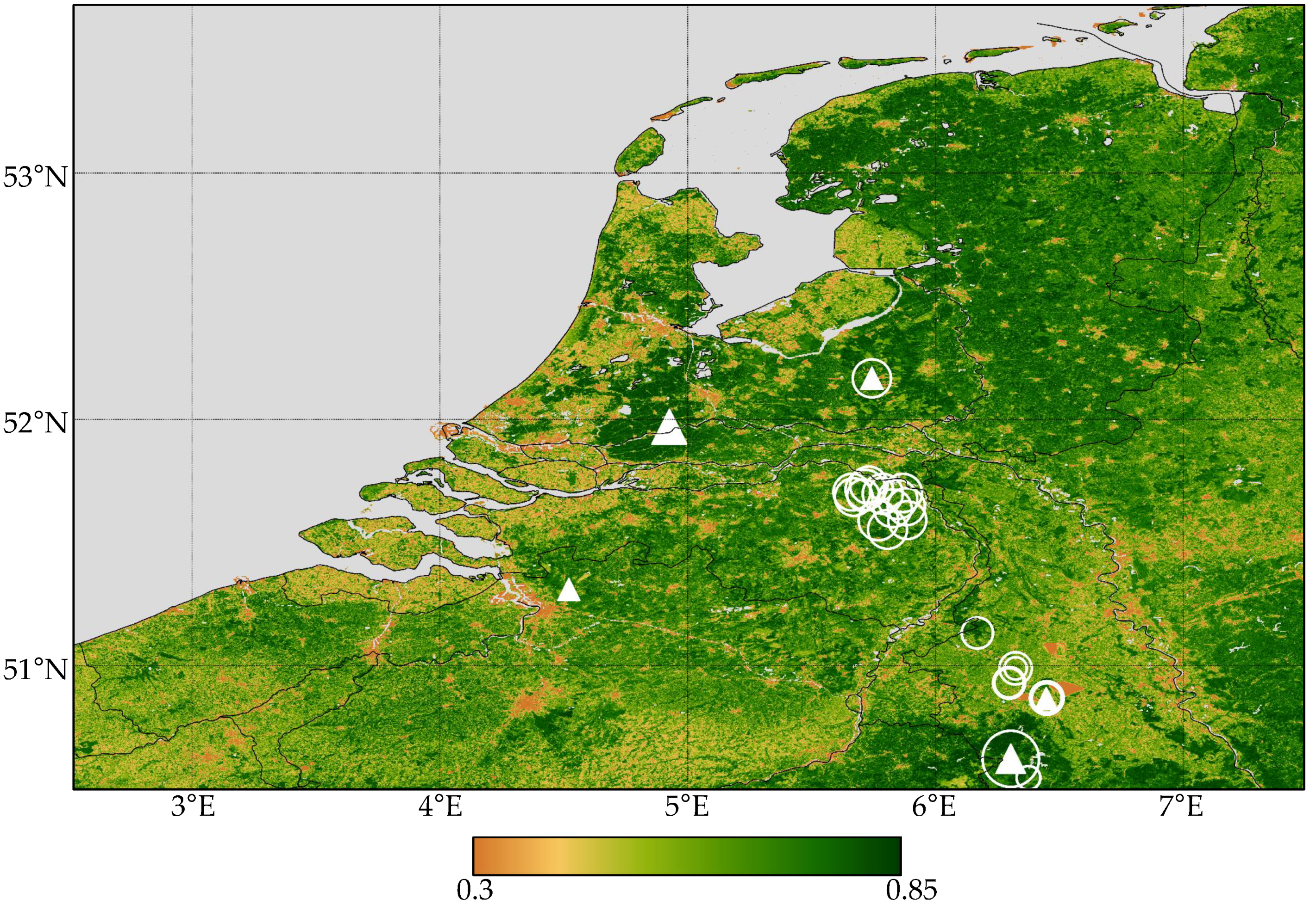
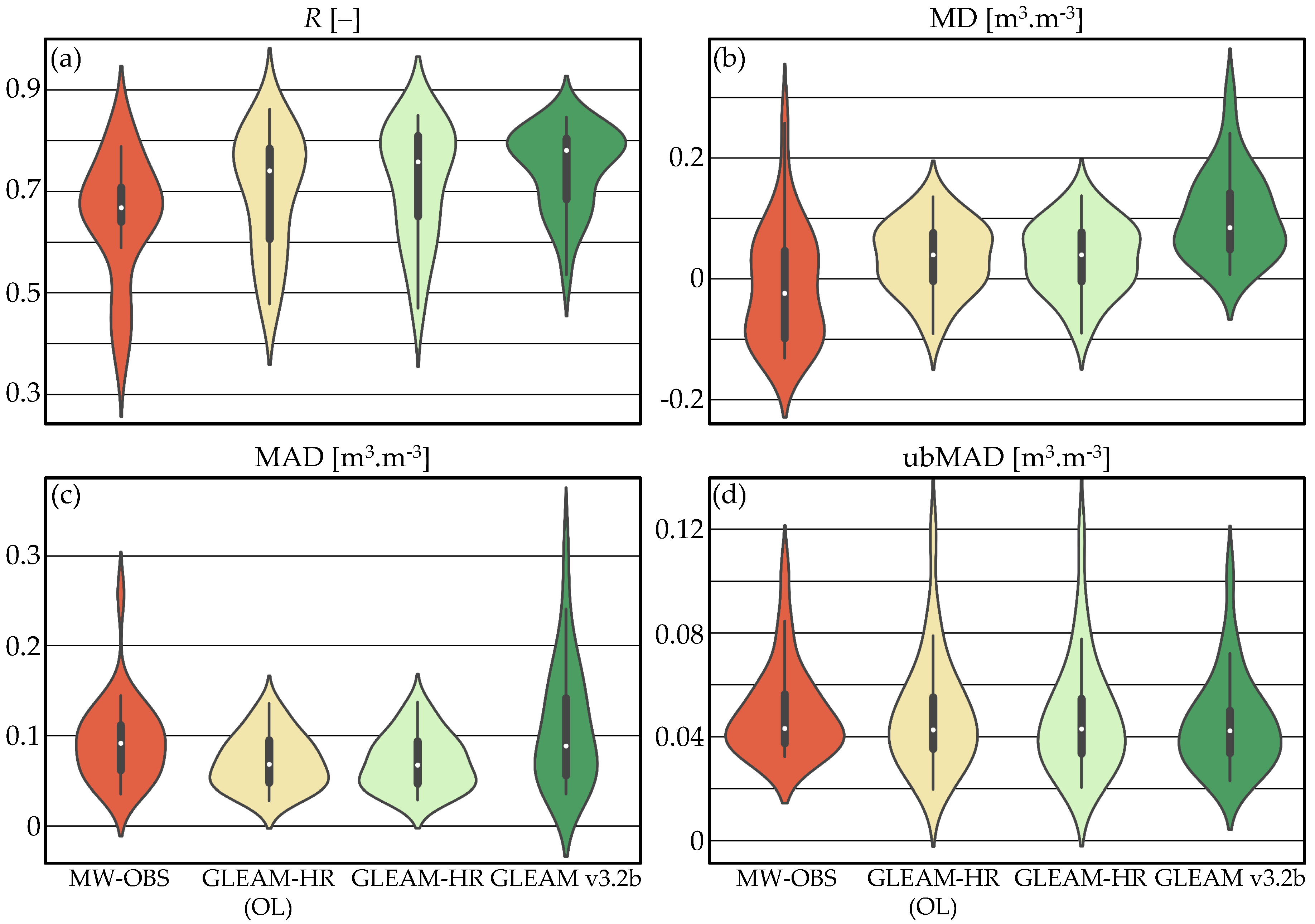
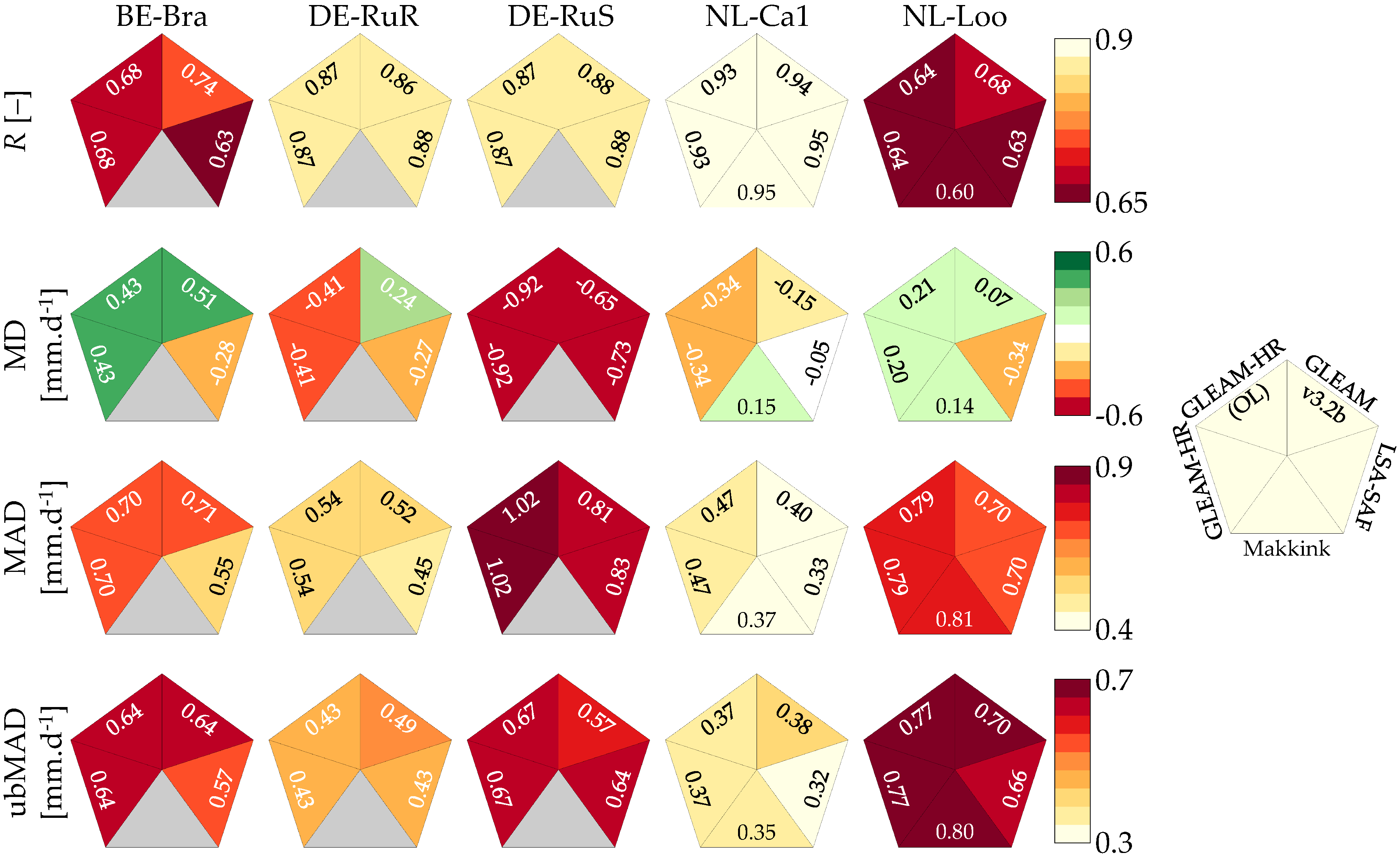
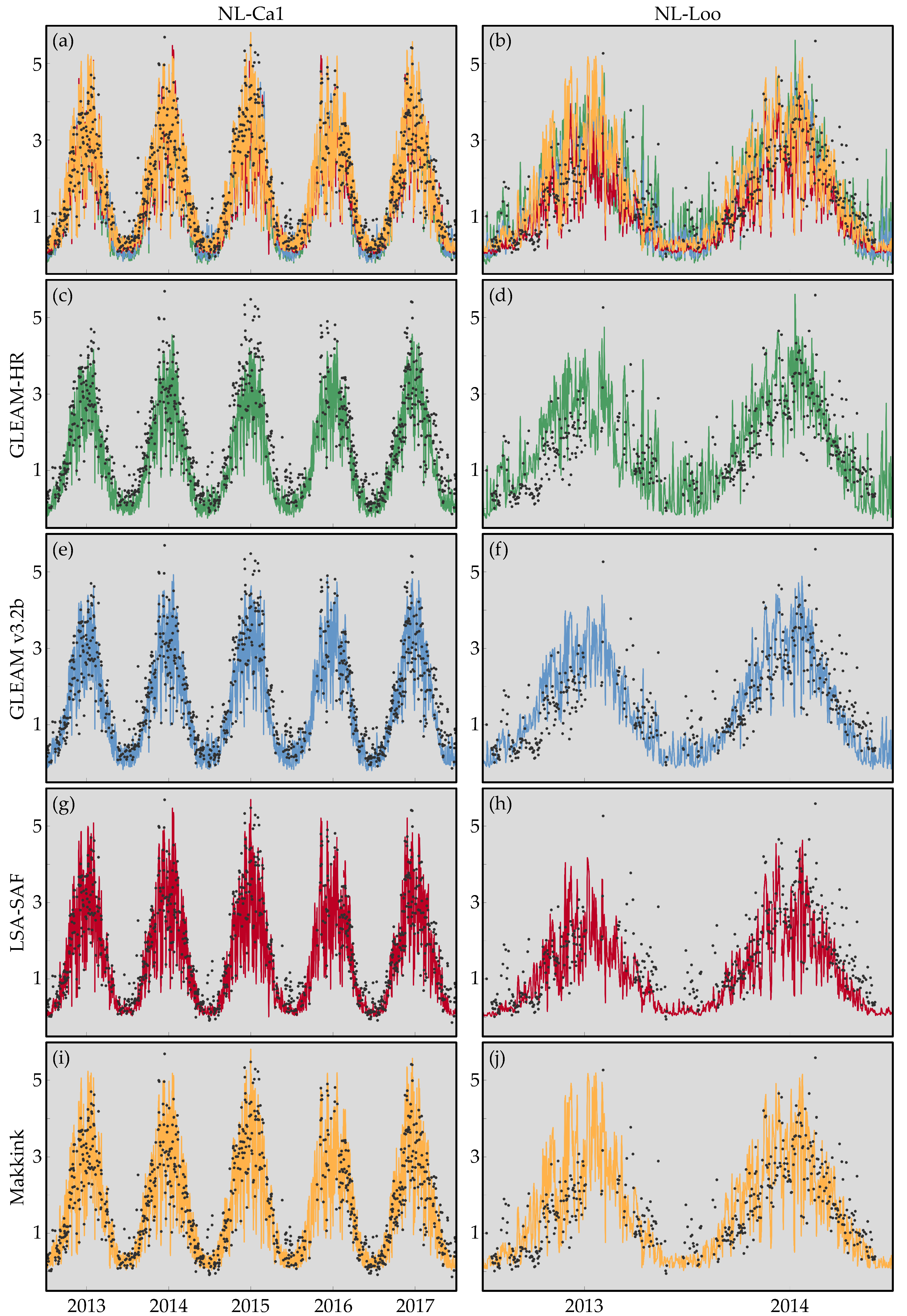
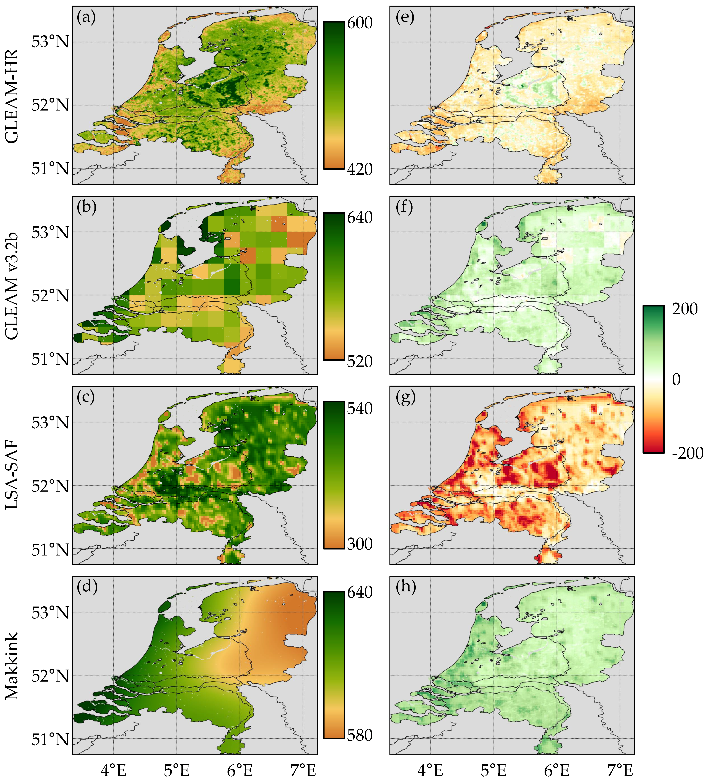
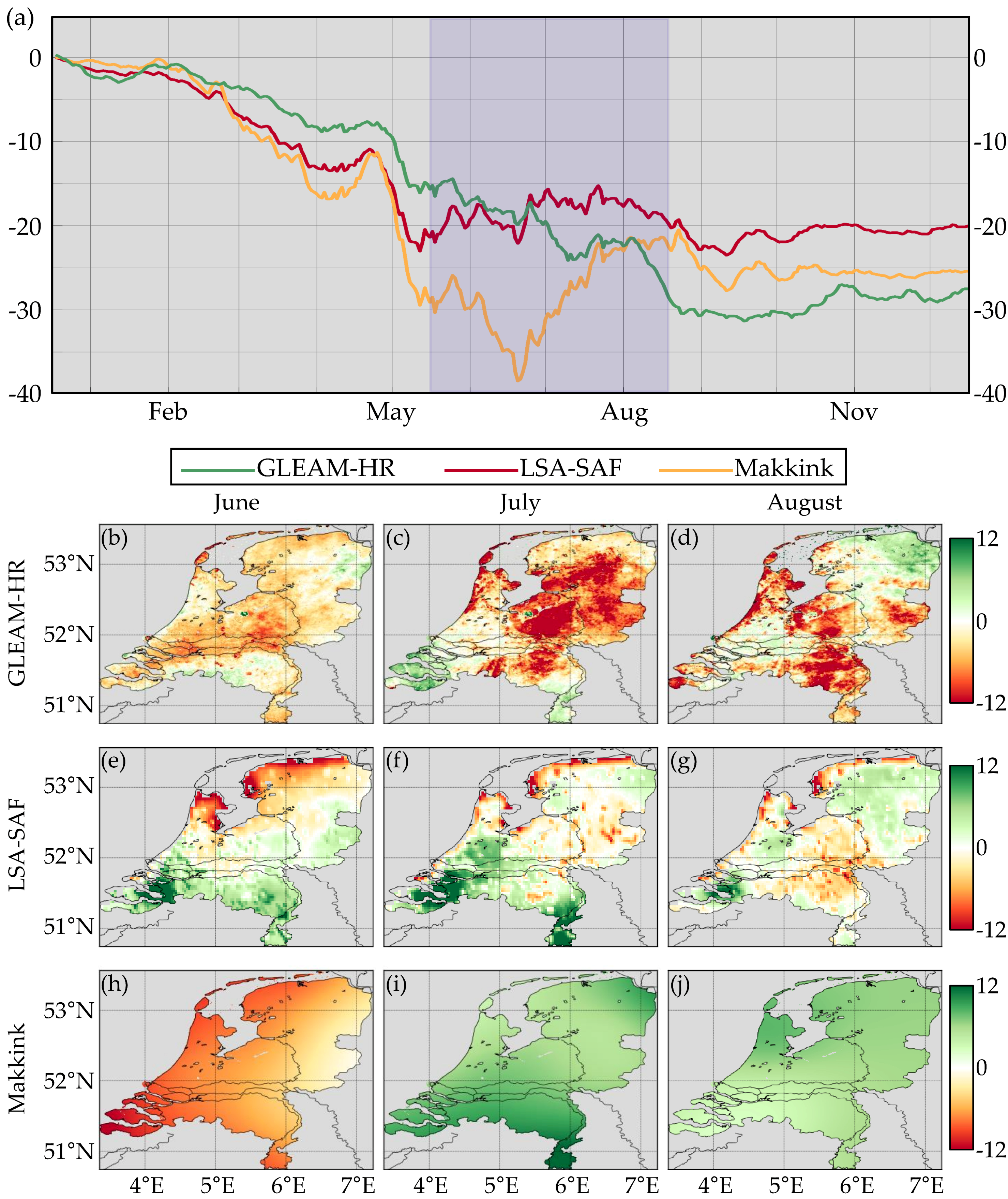
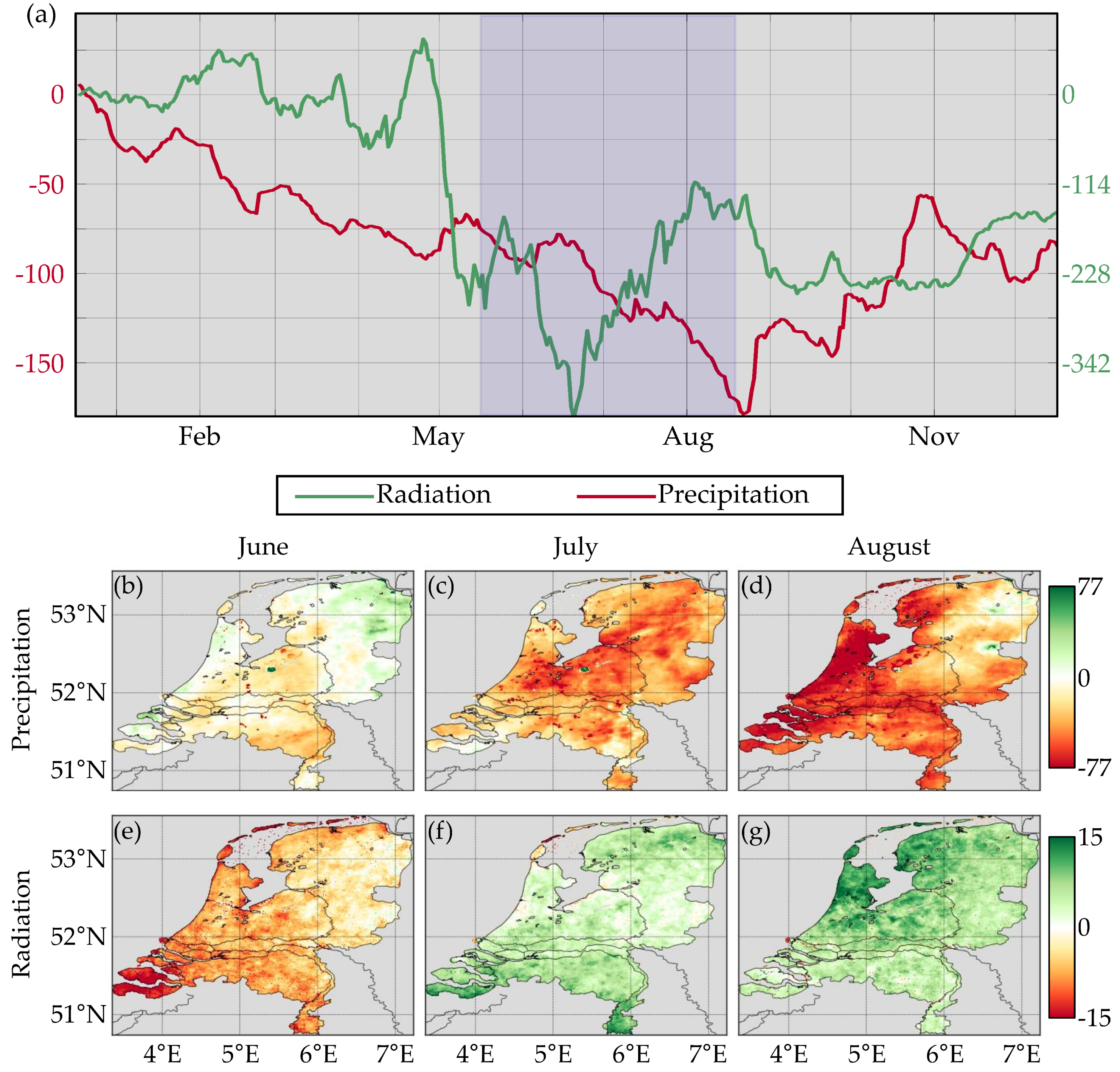
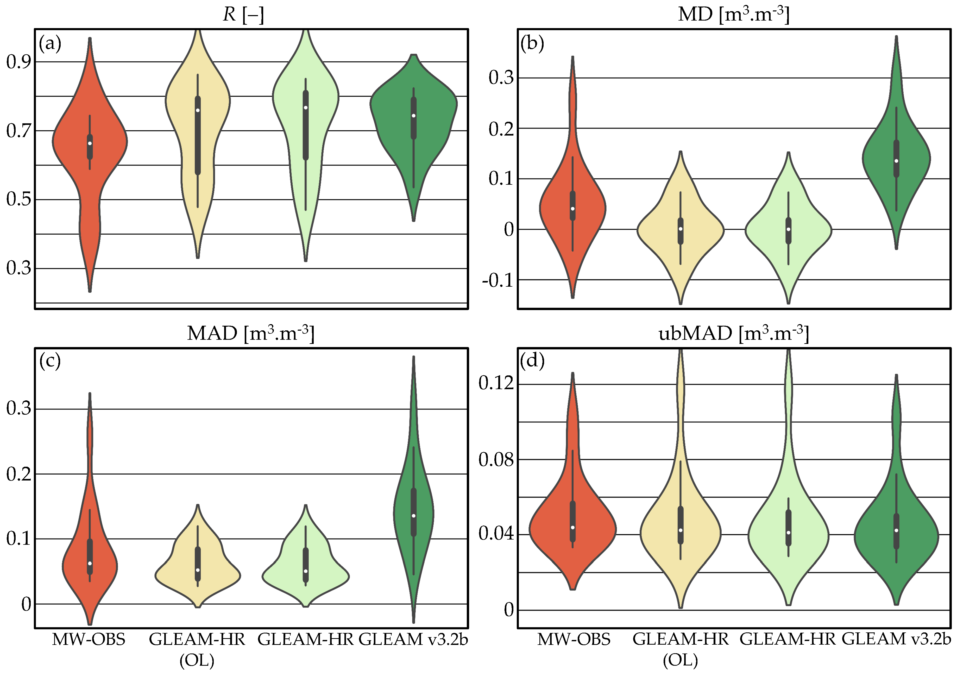
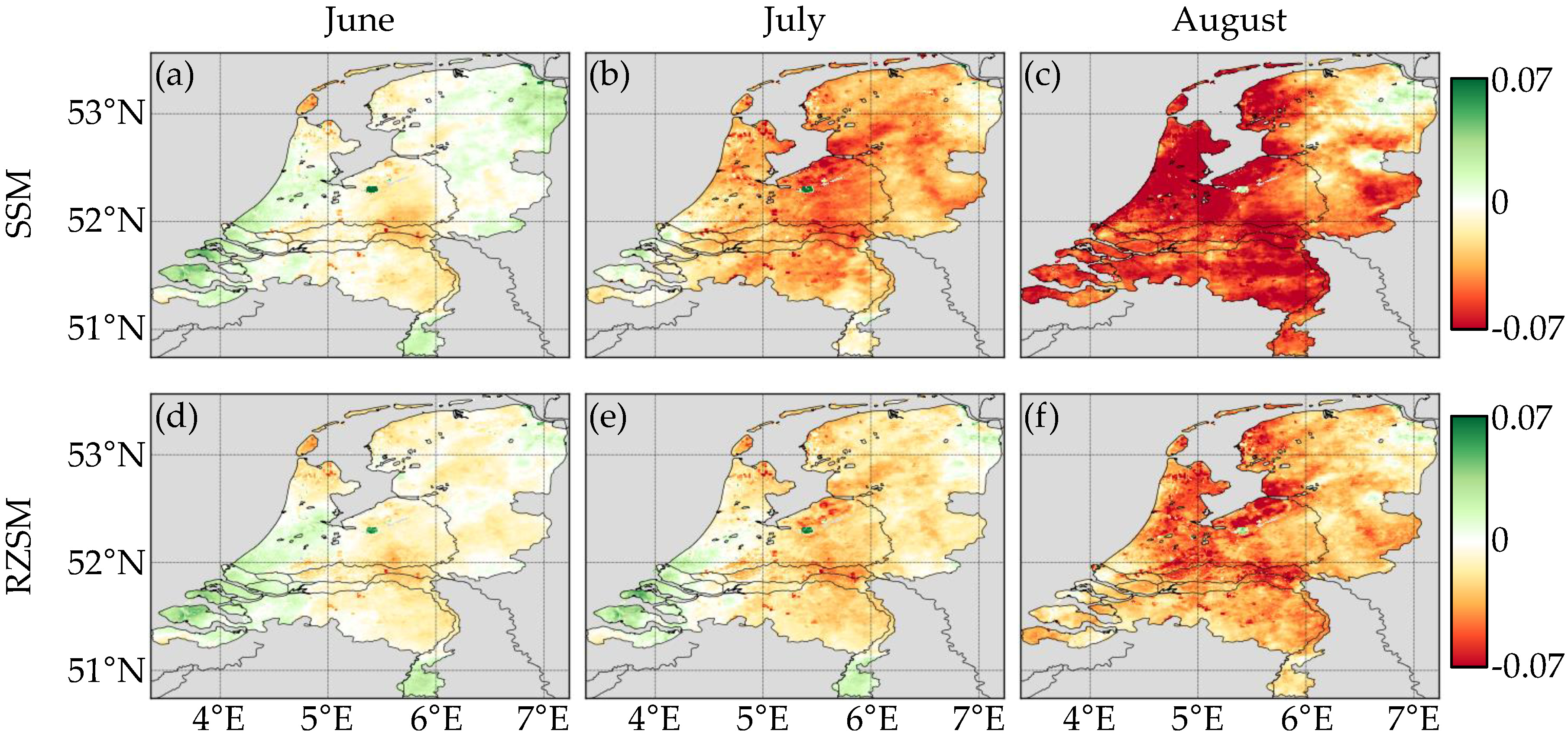
Table 1.
Datasets used to produce the forcing for GLEAM-HR together with their approximate native spatial and temporal resolution and reference.
Table 1.
Datasets used to produce the forcing for GLEAM-HR together with their approximate native spatial and temporal resolution and reference.
| Variable | Dataset | Resolution | References | |
|---|---|---|---|---|
| Spatial | Temporal | |||
| , , , | CERES L3SYN1DEG | 100 km | 1 day | Wielicky et al. [56] |
| , | Meteosat LSA SAF DIDSSF/DIDSLF | 3.1 km | 1 day | Trigo et al. [54] |
| Emissivity | Meteosat LSA SAF EM | 3.1 km | 1 day | Trigo et al. [54] |
| Albedo | MODIS MCD43A3 | 500 m | 16 day | Schaaf and Wang [55] |
| LST | VanderSat LST-100 | 100 m | 1 day | VanderSat [45] |
| Precipitation | Nationale Regenradar | 1 km | 5 min | Royal Haskoning DHV and |
| Nelen and Schuurmans [57] | ||||
| VOD | VanderSat VOD-C1N-100 | 100 m | 1 day | VanderSat [45] |
| Soil Moisture | VanderSat SM-C1N-100-SWI-T10 | 100 m | 1 day | VanderSat [45] |
| ASCAT-SWI | 10 km | 1 day | Albergel et al. [59] | |
| Cover Fractions | MODIS MOD44B | 250 m | 1 year | Dimiceli et al. [62] |
| Soil Properties | SoilGrids250m | 250 m | — | Hengl et al. [61] |
| Lightning Frequency | LIS/OTD | 5 km | — | Mach et al. [63] |
Table 2.
Eddy-covariance sites used in this study together with their FLUXNET code (ID), latitude, longitude, International Geosphere-Biosphere Programme (IGBP) land cover (LC), data coverage within the study period (number of daily measurements between brackets), and official reference (or principal investigator (PI)). * Indicates that both measurements of surface soil moisture and evaporation are available.
| ID | Latitude | Longitude | LC | Data Coverage | Reference/PI |
|---|---|---|---|---|---|
| BE-Bra | 51.31 | 4.52 | MF | 2013–2014 (187) | Carrara et al. [68] |
| DE-RuR * | 50.62 | 6.30 | GRA | 2013–2016 (334/1253 *) | Borchard et al. [69] |
| DE-RuS * | 50.87 | 6.45 | CRO | 2013–2015 (193/573 *) | Eder et al. [70] |
| Nl-Ca1 | 51.97 | 4.93 | GRA | 2013–2017 (473) | Chen et al. [71] |
| Nl-Loo * | 52.17 | 5.74 | ENF | 2013–2014 (193/576 *) | Eddy Moors |
© 2018 by the authors. Licensee MDPI, Basel, Switzerland. This article is an open access article distributed under the terms and conditions of the Creative Commons Attribution (CC BY) license (http://creativecommons.org/licenses/by/4.0/).
Share and Cite
MDPI and ACS Style
Martens, B.; De Jeu, R.A.M.; Verhoest, N.E.C.; Schuurmans, H.; Kleijer, J.; Miralles, D.G. Towards Estimating Land Evaporation at Field Scales Using GLEAM. Remote Sens. 2018, 10, 1720. https://doi.org/10.3390/rs10111720
AMA Style
Martens B, De Jeu RAM, Verhoest NEC, Schuurmans H, Kleijer J, Miralles DG. Towards Estimating Land Evaporation at Field Scales Using GLEAM. Remote Sensing. 2018; 10(11):1720. https://doi.org/10.3390/rs10111720
Chicago/Turabian StyleMartens, Brecht, Richard A. M. De Jeu, Niko E. C. Verhoest, Hanneke Schuurmans, Jonne Kleijer, and Diego G. Miralles. 2018. "Towards Estimating Land Evaporation at Field Scales Using GLEAM" Remote Sensing 10, no. 11: 1720. https://doi.org/10.3390/rs10111720
Note that from the first issue of 2016, this journal uses article numbers instead of page numbers. See further details here.