Modeling Microseism Generation by Inhomogeneous Ocean Surface Waves in Hurricane Bonnie Using the Non-Linear Wave Equation

General Dynamics—Applied Physical Sciences, Groton, CT 06340, USA
†
Work Conducted at the Massachusetts Institute of Technology, Department of Mechanical Engineering, Cambridge, MA 02139, USA.
Remote Sens. 2018, 10(10), 1624; https://doi.org/10.3390/rs10101624
Submission received: 2 July 2018
/
Revised: 30 September 2018
/
Accepted: 4 October 2018
/
Published: 12 October 2018
(This article belongs to the Special Issue Advances in Undersea Remote Sensing)
Abstract
:It has been shown that hurricanes generate seismic noise, called microseisms, through the creation and non-linear interaction of ocean surface waves. Here we model microseisms generated by the spatially inhomogeneous waves of a hurricane using the non-linear wave equation where a second-order acoustic field is created by first-order ocean surface wave motion. We treat range-dependent waveguide environments to account for microseisms that propagate from the deep ocean to a receiver on land. We compare estimates based on the ocean surface wave field measured in hurricane Bonnie in 1998 with seismic measurements made roughly 1000 km away in Florida.
1. Introduction
Hurricanes generate seismic noise, commonly referred to as microseisms, in the 0.1 to 0.6 Hz frequency range. On a few occasions measurements of these microseisms have been used to track hurricanes [1,2,3,4,5,6,7,8]. More generally these microseisms are a significant cause of noise in seismic measurements [7,9,10] and raise the detection threshold for monitoring earthquakes [11].
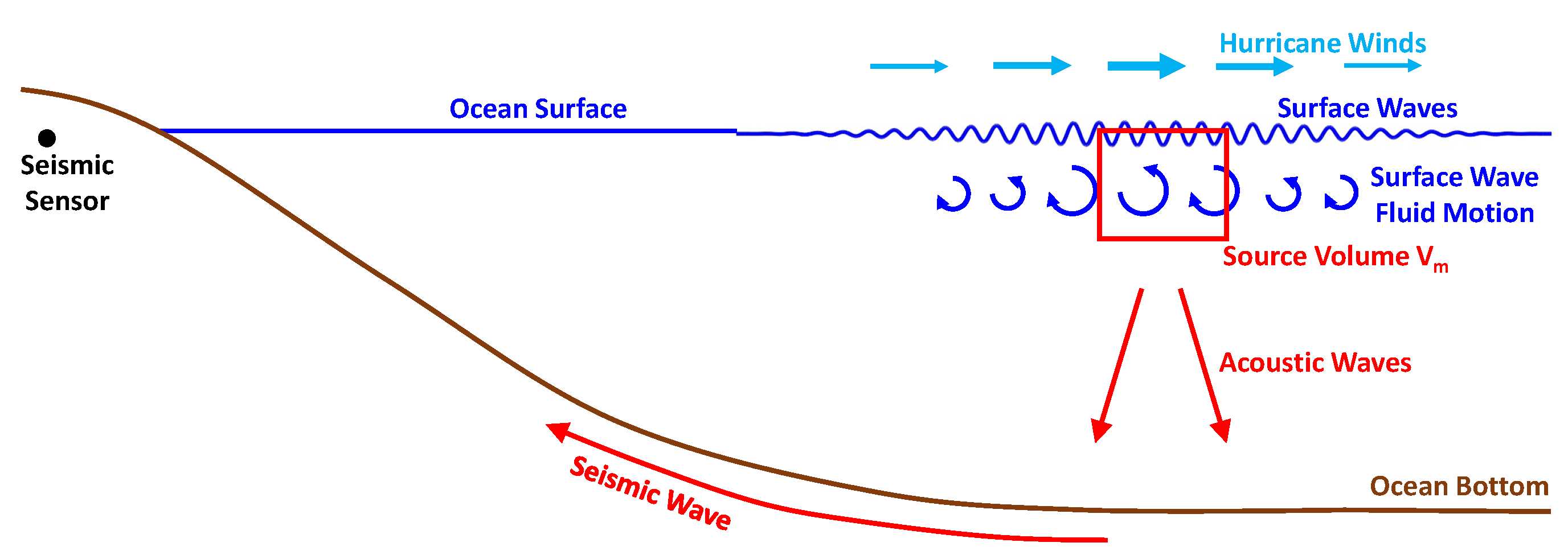
Physically the process for generating microseisms can be broken down into four steps: (1) The spatially and temporally varying hurricane winds create complicated wave patterns on the ocean surface; (2) In locations where these surface waves are in opposition, their non-linear interactions generate acoustic waves; (3) These acoustic waves propagate through the water and couple into the ocean bottom; (4) The resulting seismic waves propagate along the sea bottom where they may be detected at great distances by seismic sensors. In this paper we develop an approach for estimating the microseisms generated by a hurricane and their seismo-acoustic propagation.
Our modeling approach is based on the non-linear wave equation where a second-order acoustic field is generated by a source distribution that depends on the first-order ocean surface wave motion. The acoustic (or seismic) field at a receiver can then be expressed as the integral over the source distribution multiplied by the waveguide Green function. This approach is ideal for hurricane-generated microseisms since it can be applied to spatially inhomogeneous surface wave fields. Also, this approach may be used in range-dependent waveguide environments as is the case when a hurricane at sea generates microseisms that propagate up the continental margin to a receiver on land.
As an example, we use the ocean surface directional wave spectrum from hurricane Bonnie [12,13] to estimate the microseismic source levels. We than calculate the Green’s function to describe the seismo-acoustic propagation from Bonnie’s location in the North Atlantic to a seismometer in Florida. Our calculated levels are then compared against actual measurements.
Our approach builds on a long history of microseism modeling efforts. Initially, microseism generation was modeled for idealized situations [14] where the ocean surface wave field was taken to be spatially homogeneous and the ocean waveguide to be range-independent. Previous microseismic models, however, cannot be applied in typical hurricane scenarios because the surface wave fields are inhomogeneous in that the wave height spectra in different parts of the hurricane can vary both in magnitude and directionality. In some cases this is because spatial homogeneity is assumed over infinite [15,16,17,18,19,20] or very large [14,21,22] surface wave areas. One model that does account for finite microseismic source generation regions is limited by the assumption that the receiver is at the center of the source area [23,24]. Also, these previous models are not applicable to the range-dependent environments typical in hurricane measurements where microseisms generated by a hurricane over the deep ocean are measured by sensor on land. Our non-linear wave equation method is shown to agree with earlier models [18,20] if we make the same simplifying assumptions that the source generation region is spatially homogeneous and that the waveguide can be modeled as an infinite half-space.
While the treatment of inhomogeneous surface wave fields and range-dependent waveguides presented here had not been previously considered, the medium non-linear wave equation used here has a parallel derivation to the wave equations or hydrodynamic equations used in earlier works. Longuet-Higgins [14], Hasselmann [17] and Brekhovskikh [15] base their derivations on perturbing Bernoulli’s equation while Hughes [18] and Kibblewhite and Wu [19] begin by separately perturbing the equations of momentum, continuity and state. We show that the non-linear wave equation used here is equivalent to perturbation expansions [18] for the physical parameters typical in hurricane microseisms. Lloyd [20] and Cato [23] base their derivations on Lighthill’s equation; however, Lloyd [20] shows that both perturbation and Lighthill approaches yield the same end result. We also note that the non-linear wave equation can be derived as a second-order approximation of Lighthill’s equation [25].
These second-order non-linear theories should not be confused with the linear theories proposed by Banerji [26] and Bowen et al. [27]. These linear theories claim that the first-order motion of a surface gravity wave creates a first order pressure fluctuation on the sea floor regardless of how deep the ocean is. This is contrary to classic surface wave theory which shows that first-order wave motion decays exponentially with depth such that, in deep water, the first-order pressure fluctuation on the sea floor goes to zero [14,28,29,30].
Our derivation is in agreement with earlier works [14,31], which show that microseisms are generated by the non-linear interaction of ocean surface waves with roughly the same wavelength but opposing propagation directions. Measurements [13,32] and models [12] of surface directional wave height spectra in hurricane Bonnie show complex patterns with the opposing surface waves necessary to generate microseisms. Based on the wave height spectra in hurricane Bonnie, we calculate the microseismic source levels generated by the non-linear interaction of the ocean surface waves.
It has been shown both theoretically [10,14] and experimentally [4,11,33,34,35,36,37] that microseisms propagate as Rayleigh waves along the sea floor. Here we develop a normal-mode model for the propagation of Rayleigh waves along the seafloor assuming a water depth that changes with range. The Green’s function from this model is used to estimate the propagation of the microseism from deep water to a seismometer on land.
Given the wave height spectra in hurricane Bonnie, the calculation of the microseismic source level generated by the non-linear wave interaction, and the propagation of those waves along the sea floor, we estimate the noise levels at a seismometer in Florida. These estimates are then compared against measured data.
It should be noted that there are other sources of microseisms besides hurricanes. Microseisms have been associated with other non-hurricane storms, coastal regions where complex wave patterns are prevalent, and the typical ambient ocean wave spectra [11,38,39,40,41,42,43,44]. These other sources of microseisms are not considered here.
2. Materials and Methods
2.1. Ocean Surface Gravity Waves
Hurricanes are characterized by high winds that can vary quickly with position, both in direction and speed, as shown in Figure 1A. In addition a hurricane may move at speeds up to 15 m/s [45] so that the winds at any location can also change with time. These spatially and temporally varying winds generate complex ocean surface wave directional spectra Figure 2 with wave heights that can exceed 10 m [12,13,32].
For surface gravity waves that are homogeneous over an infinite ocean surface area we can express the complex surface wave height as the linear superposition of plane waves [46] where is the sea surface wavenumber and is the corresponding frequency where in deep water . Throughout this paper the surface wavenumber is expressed either in cartesian coordinates as or in polar coordinates as . Also, a cartesian coordinate system is used for position where where z is defined downward from the sea surface. The complex surface wave height can then be written as
where is the surface wave height spectrum.
Since the complex wave height is produced by the contributions of many independent random physical processes, we can assume by Central Limit Theorem that the statistical distribution of is Gaussian [47]. In addition we may define the reference position from which wave height is measured such that has zero mean. Given this assumption, in Appendix A.1 we show that must also be a zero-mean complex Gaussian random variable [46,47].
Since the spectrum is zero-mean and homogeneous over an infinite ocean surface area, the second moment of the spectrum can be written as (see Appendix A.1) [16,47,48]
where denotes the expectation. This expression shows that, for stationary processes, the wavenumber components and decorrelate. Also, since the spectrum is Gaussian, the fourth moment can then be written as [16]
In a hurricane the surface waves are not homogeneous over an infinite area, but rather the surface wave spectrum changes gradually with position in the storm. To characterize the spatially varying surface wave field in the hurricane, we divide the sea surface into a grid made up of finite regions m with surface areas over which the wave spectrum can be taken to be homogeneous. The complex wave height in a particular finite region m then can be expressed as
In Appendix A.2 we show that the finite size of the regions m introduces a ‘windowing’ effect when calculating the moments of the spectrum . However, we also show that this windowing effect can be neglected if the dimensions and of the region are much greater than the wavelength of the surface wave. For the hurricane waves of interest in this paper, the surface wavelengths range from roughly 100 to 300 m requiring that the dimensions and be in the order of 1 km or greater. Provided this condition is met we can make the approximation.
where is the cross-spectral density of the surface wave fields at locations m and n.
As before we can assume by Central Limit Theorem that is a zero-mean complex Gaussian random variable so that is also a zero-mean complex Gaussian random variable. Because of this we can write the fourth moment as
This expression for the fourth moment of the wave height spectra will be used later in Section 2.3.
From Equation (4) we can write the real part of the surface wave height as
We can also express the real surface wave particle velocity as a linear superposition of plane waves such that
where , and represent unit vectors in the x, y and z directions respectively.
Experiments by Forristall et al. [49] show that the linear wave theory of Equations (1), (4), (7) and (8) is adequate to describe surface waves even in high sea states with significant wave breaking as in a hurricane. The use of linear surface wave theory can also be justified since the typical surface wave heights in a hurricane are an order of magnitude less than the wavelength [12,13,32,49].
Wright et al. [13] and Walsh et al. [32] measured the spatial variation of the directional wave spectra in hurricane Bonnie using an aircraft-mounted Scanning Radar Altimeter (SRA). These measurements, however, are limited to the locations and times of the aircraft flights and do not give a complete picture of the wave field in the hurricane.
To quantify the surface wave field at any location and time in hurricane Bonnie, Moon et al. [12] used the Wave Watch III (WW3) ocean surface wave model [50]. These model results, shown in Figure 2, are in close agreement with measurements from [13,32] and with data from buoys and oceanographic stations. In this paper we use the surface directional wave spectra in hurricane Bonnie calculated using WW3 [12].
2.2. Non-Linear Wave Equation
The non-linear wave equation [51,52] describes the second-order acoustic wave field generated by first order fluid motion. For the long surface waves in a hurricane viscosity may be neglected so that the non-linear wave equation can be written as [53]
where the first order velocity and pressure terms on the right-hand side generate a second-order acoustic pressure field on the left-hand side, c is the sound speed, is density and is the coefficient of nonlinearity [51,53].
In this work we will consider the case where the first order velocity , from Equation (8), is due to surface wave motion. The first order pressure can be found using conservation of momentum where . Using the relationship between first order velocity and pressure we can compare the relative magnitudes of the source terms in Equation (9). Given typical parameters to rad/m, to rad/s, m/s, kg/m, and [54] we find that the term of Equation (9) exceeds the other source terms by several orders of magnitude. Dropping the lesser terms yields
This equation is equivalent to the perturbation expression used in the previous microseism derivation of Hughes [18]. This can be seen by taking Equation (10) of [18] and assuming irrotational flow () and continuity (). Taking the Fourier Transform of Equation (10) we find the frequency domain Helmholtz equation for the second-order field
We will begin by solving for the pressure field generated by a finite volume with a source distribution which depends on the fluid velocity from Equation (8). The volume extends vertically from the ocean surface at to a depth well below the surface wave region (). The volume extends over the horizontal area with dimensions and centered at as defined in Section 2.1. We can solve the Helmholtz (Equation (11)), using the frequency domain Green function such that,
where and are the source and receiver locations respectively.
It should be noted that, although the ocean surface is perturbed by the presence of surface waves, we choose to define the upper boundary of our volume by the quiescent surface following the example of Lloyd [20]. He argues that the Green function g “has the form where is the Green function for the quiescent ocean and where , , is of degree j in a wave height perturbation parameter . The first-order term represents Bragg reflected by the moving spatially periodic components”. He shows that the terms for may be omitted in the excitation of . He goes on to apply the Green function for a quiescent ocean half-space and, even with this approximation, matches the result of earlier work by Hughes [18]. In Appendix C we will demonstrate agreement between our end result and that of both [20] and [18].
Equation (12) can be rewritten as
where the window function is unity for and and zero elsewhere. The double integral over represents the field at a receiver due to a distribution of sources q over a finite area defined by the window function w. If the receiver is in the far field of the finite area ( and where is the acoustic wavelength and where ), we can make the plane wave approximation,
where the acoustic wavenumber is defined in cartesian coordinates as where . In free space this would simplify to
however, we will use the more general form given in Equation (14). Inserting Equation (14) into Equation (13) yields
Again the double integral over analogous to a horizontal planar array of acoustic sources with broadside directed down toward the ocean bottom. In the following analogy we can define this double integral as the array output [55]
The array output in Equation (17) can be evaluated for any horizontal wavenumber vector ; however, only those wavenumber vectors where lead to a propagating acoustic field. This can be illustrated if we consider the microseismic field generated by a horizontal plane of sources near the sea surface as described in Equation (17). In previous works [14] it has been shown that microseisms generated at the ocean surface are first transmitted downward to the sea floor where they then propagate along the bottom as Rayleigh waves. This vertical propagation from the sea surface to the sea floor can be modeled to first order using the free-space Green function
where d represents the water column depth. If exceeds then becomes imaginary leading to an exponential decay with depth d. For example if then so that, for rad/s, m/s and an ocean depth m, the field is attenuated by or 13 dB. Greater depths will lead to even more attenuation. Because of this evanescent attenuation we will only consider the acoustic field where .
Assuming the acoustic pressure field given in Equation (16) is temporally stationary, the power spectral density may be written as [56]
where represents the expectation and . In the next section we derive expressions for the second moment of the array output and the power spectral density due to ocean surface waves.
The power spectral density in Equation (19) represents the field at a receiver from a single pair of finite volumes and . In the next section we determine the microseismic field generated by a hurricane where the surface wave field is inhomogeneous and extends over a large region hundreds of kilometers across. To do this we divide the hurricane region into finite volumes , as shown in Figure 3, and then sum their contributions to find the total power spectral density of the received field written as
2.3. Power Spectral Density Due to Ocean Surface Gravity Waves
Taking the ocean surface wave velocity as the first order field we can determine the source term from Equation (11) where is the Fourier transform
of
Given Equation (8) for the first order velocity we find
where , , , and . Note that the Laplacian operator () in Equation (23) leads to the direction cosine functions
and
where , , , and .
Substituting Equation (23) into the definition of from Equation (22) and taking the Fourier transform yields,
Note that the wave height spectra and in Equation (27) can be brought out of the spatial integral since they are constant over the ocean surface area defined by the window function w. Integrating over then leads to
where ∗ represents the two-dimensional convolution written as,
and where
Note that, when integrating over , the term in the window function of Equation (27) introduces a phase factor . This cancels the other phase term in Equation (27). From this we see that the source array output given in Equation (28) has no phase dependence on location .
The delta functions in Equation (28) show that the horizontal component of the acoustic wavenumber vector is generated by and equal to either the sum or difference of the surface wavenumber. In Section 2.2 we discussed how the non-propagating field where is not significant and may be ignored. Therefore, when integrating over we need only consider a range of integration corresponding to propagating acoustic waves. For the sum terms in Equation (28) corresponds to the integration region where and for the difference terms corresponds to .
Here we will define the source area dimensions and to be ‘acoustically small’ (). The acoustic wavelengths of the microseismic field in water range from roughly 6 to 11 km requiring that the dimensions and be on the order of 1 km or less. Note that this requirement on and , combined with the requirement that from Section 2.1, means that . If , the function in Equation (30) within the range of acoustically propagating wavenumbers . With this approximation Equation (28) can be written as
The power spectral density of the pressure in Equation (19) contains the second moment or variance of the array output which from Equation (31) can be expressed as,
Since the wave height spectra and are uncorrelated zero-mean Gaussian random variables as discussed in Section 2.1, we can substitute Equation (6) into Equation (32) and integrate over and to obtain
Then by integrating in Equation (33) over the integration region , corresponding to and , we find
Since this integration leads to the approximations in the sum terms and in the difference terms.
The term of Equation (34) leads to a constant value in the power spectral density that is irrelevant. Also, for the remainder of the paper, we suppress the subscripts of and to simplify notation.
The wave height cross-spectral density can be converted to the frequency-angle (-) domain by evaluating the Jacobian where [57]. This yields the relation . Making this substitution in Equation (34) and integrating over yields,
Note that the delta functions in Equation (34) introduce a frequency doubling effect in Equation (35) where the frequency of the acoustic wave is twice the frequency of the surface gravity wave.
Substituting Equation (35) into Equation (19) and integrating over leads to the power spectral density of the pressure field
where we define the ‘microseismic source cross-spectral density’ as
Summing the contribution from all finite volumes gives us the total received power spectral density
Equation (38) provides an analytic expression for microseisms generated by inhomogeneous ocean surface wave fields, as opposed to previous formulations where spatial homogeneity is assumed over infinite [15,17,18,19,20] or very large [14,21,22] surface wave areas. Also the Green functions and in Equation (38) may be calculated for any arbitrary range-dependent or range-independent ocean waveguide using standard propagation models. Later we will use a formulation for range-dependent Rayleigh wave propagation to calculate the Green functions and model microseismic propagation in a typical North Atlantic waveguide environment.
While Equation (38) is applicable to inhomogeneous surface wave fields and arbitrary ocean waveguides, it can also be applied to simpler homogeneous surface wave fields and Green functions. In fact, in Appendix C we find that, given an infinite half-space and assuming the surface wave spectrum is range-independent (), the power spectral density of the pressure field in Equation (38) simplifies to the results derived by Hughes [18] and by Lloyd [20].
2.4. Microseismic Source Levels in Hurricane Bonnie
In this section we show how Equation (37) can be used to find the microseismic source cross-spectral density generated by the surface wave field in a realistic hurricane. In these examples we use the wave spectra from hurricane Bonnie. Through this analysis we demonstrate the relationship between the wind speeds, surface wave spectra, and microseismic source spectra in a hurricane.
Beginning on 22 August 1998, hurricane Bonnie traveled along the east coast of the Bahamas, Florida, and South Carolina [58]. During this time microseisms were recorded by an Incorporated Research Institutions for Seismology (IRIS) seismometer at the Disney Wilderness Preserve in Florida (N, W). Here we model the microseisms generated by hurricane Bonnie that would be measured by this seismometer.
To evaluate the microseismic source cross-spectral density of Equation (37) requires knowledge of the surface wave height spectrum . Moon et al. [12] calculate the surface wave height spectrum for the wind speeds measured in hurricane Bonnie using the Wave Watch III (WW3) wind-wave modeling program [50]. They also show how their results are in close agreement with aircraft-based measurements of surface wave height spectrum by Wright et al. [13] and Walsh et al. [32].
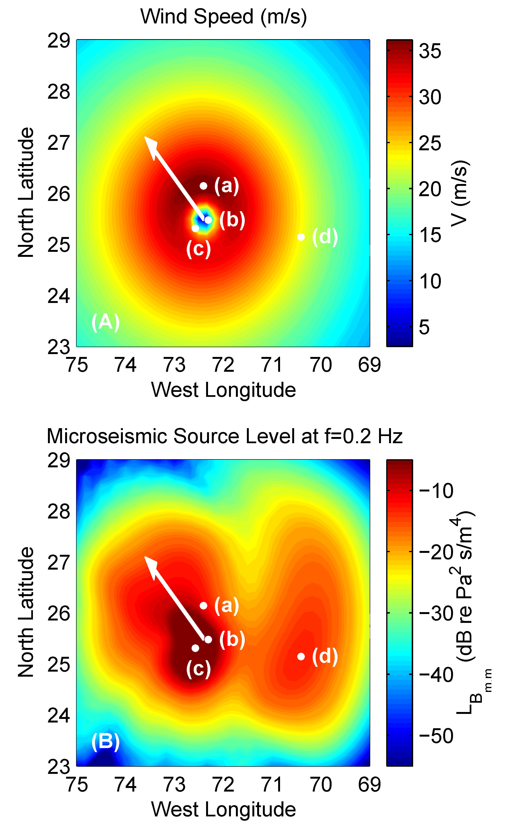
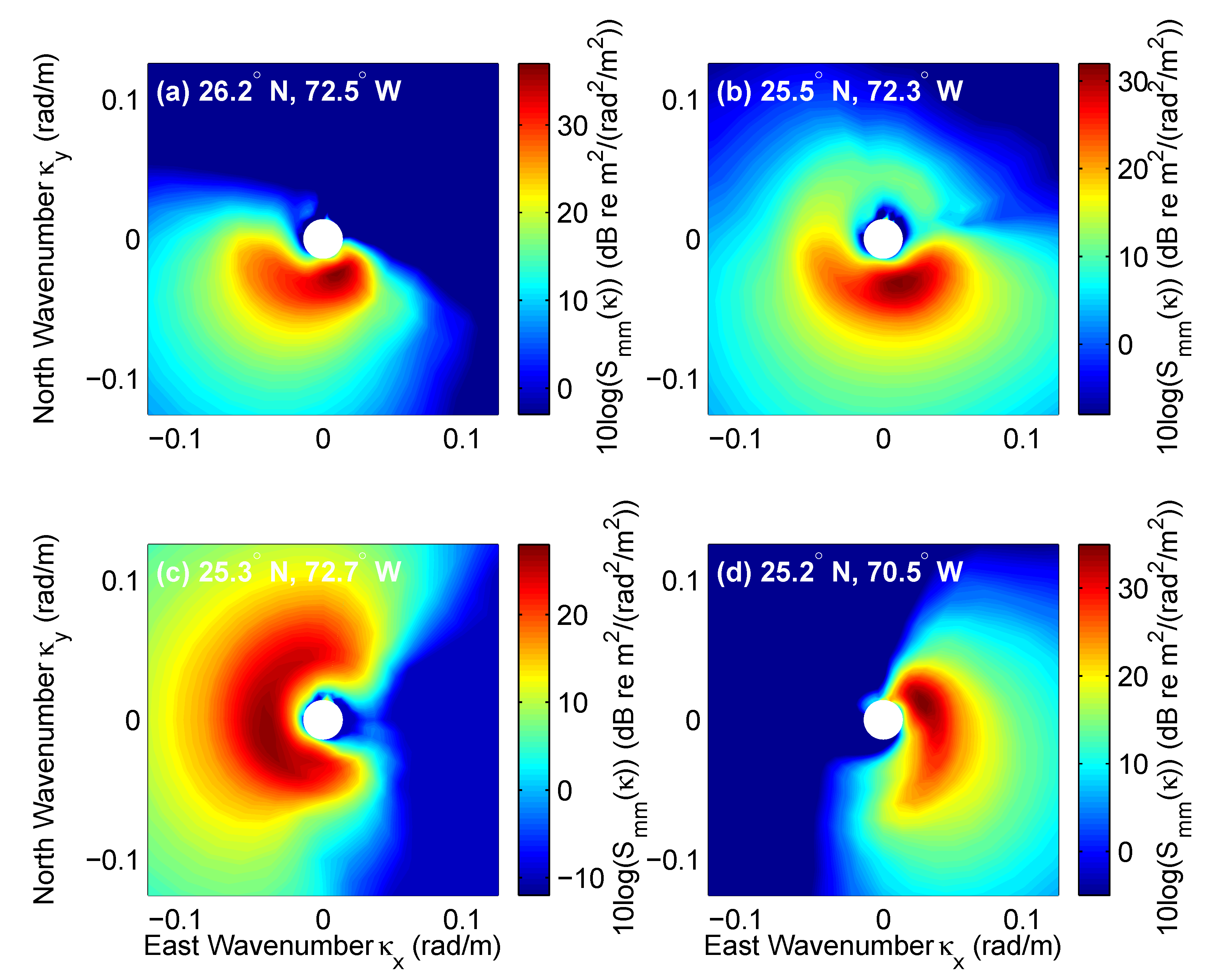
Figure 1A shows the surface wind speed in hurricane Bonnie on 24 August 1998. Illustrated is the typical hurricane structure with the high wind speeds of the ‘eye wall’ surrounding the ‘eye’ at the hurricane’s center. From these wind speeds, WW3 is used to determine the wave height spectra as defined in Equation (5) (Figure 2). In Figure 2 we see that hurricanes generate waves that propagate in many different and often opposing directions. For example in Figure 2c we see a peak in the surface wave spectrum (in red) with waves traveling North (), West (), and South ().
From the wave height spectra calculated using WW3, the microseismic source cross-spectral density may be calculated from Equation (37). We define the ‘microseismic source level’ as
expressed in dB re where the somewhat arbitrary length scales and have been factored out. Figure 1B shows at rad/s ( Hz) on 24 August 1998, the day where we found the source level to be highest. We see that the peak of at location (c) is not at the same location as the maximum wind speed (a). This is because, while location (a) has large wave heights (≈37 dB re ), the waves are all propagating primarily to the South without any opposing waves. At location (c), however, there are opposing waves (propagating both North and South) which generate microseisms as expressed in Equation (37). Also the source level is higher in the low-wind-speed eye (b) than at the maximum wind speed location (a) due to the opposition in the surface waves (Figure 2b).
The arrows in Figure 1 represent the direction hurricane Bonnie was moving and we see that there is a small peak in the source level well ‘behind’ the hurricane at location (d) even though the wind speed there is relatively low. This is again due to the opposing waves at this location (Figure 2d). This illustrates the complex relationship between wind speed and wave spectra, where the wave spectra is a function not only of wind speed but also of hurricane geometry and translation speed [12], and the complex relationship between wave spectra and microseismic source level, where the level depends on the non-linear interaction of opposing waves.
3. Results
In this section we model the propagation of the microseisms generated by hurricane Bonnie through the North Atlantic waveguide. The model results are then compared with seismic data gathered in Florida.
To determine the microseisms received at the sensor in Florida the Green functions and of Equation (38) are calculated using the adiabatic Rayleigh wave propagation model derived in Appendix B. The bathymetry between the hurricane, located over the roughly 5 km deep Hatteras Abyssal plain on 24 August, and the seismometer, located in Florida is characterized by a gentle upslope. We will model this up-sloping environment with the simplified geometry shown in Figure 4. The sound speeds and densities for this model waveguide are based on typical values for the deep North Atlantic Ocean [59] and bottom [60].
With this environment the Green functions and are calculated using Equation (A47). The sea-floor depth at the center of hurricane Bonnie is given in Table 1, as well as the range between the seismometer and the hurricane center. The seismometer in Florida is buried in the ground to a depth of 162 m as shown in Figure 3.
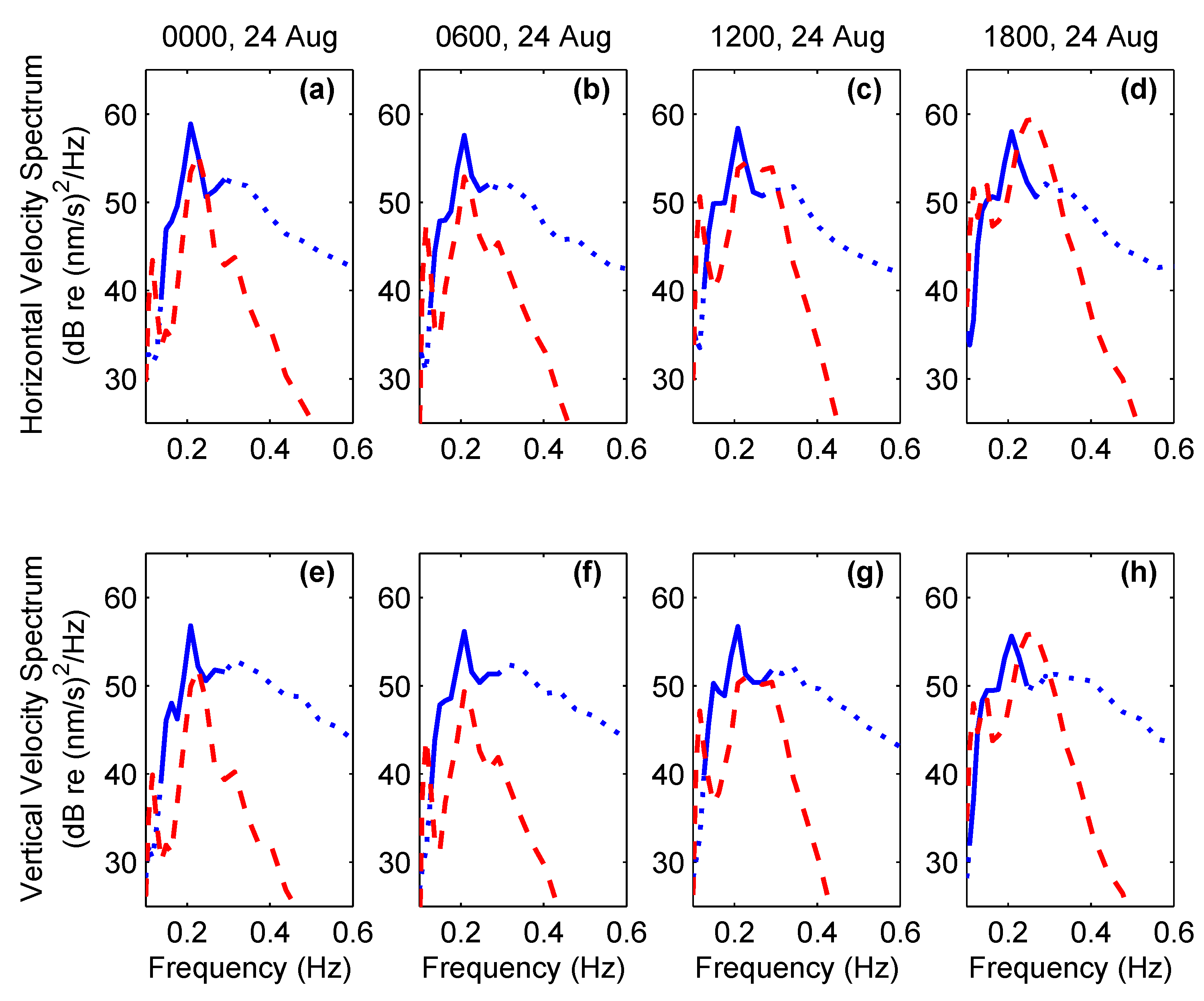
Given the source cross-spectral density from Equation (38) and Green functions from Equation (A47), the power spectral density of the field, from Equation (38), received by the seismometer in Florida is calculated. Figure 5 shows the power spectral density of the horizontal velocity (Figure 5a–d) and vertical velocity (Figure 5e–h) of the earth’s crust at the Florida seismometer based on our model (the red dashed curves) and on measured data (in blue).
The dotted blue lines in Figure 5 represent portions of the measured data that are dominated by non-hurricane related ambient noise. The level of this ambient noise is determined by measuring the noise levels during the week before and the week after the hurricane passed. The un-corrupted microseism signals are taken to be those that exceed the ambient by at least 3 dB while anything below that is considered to be corrupted.
4. Discussion
The theoretical results and measured data show reasonable agreement with peaks in the spectrum at roughly Hz and a peak level between 50 and 60 dB re . Note that the peak of the wave height spectral in Figure 2 is at roughly rad/m which equates to a surface wave frequency rad/s. From the frequency doubling effect discussed in Section 2.3, this gives a peak in the acoustic field at rad/s or Hz which we see in the received field in Figure 5.
There is a lesser peak in the model result at around 0.1 Hz that is not obvious in the measured data. This peak in the model comes from the model for the Rayleigh wave propagation and suggests perhaps a limitation of the single layer (fluid water layer over a solid half-space) approximation adopted here.
It should be noted that the horizontal- and vertical-velocity measurements are consistent with Rayleigh waves. There is no evidence that other seismic wave types play a significant role.
5. Conclusions
Here we present an analytic model, based on the non-linear wave equation, to describe the microseisms generated by a hurricane. This model is ideal for hurricane-generated microseisms since it can be used to calculate the acoustic field due to spatially inhomogeneous surface waves. Also, this model may be used in range-dependent waveguide environments as is the case when a hurricane at sea generates microseisms that propagate up the continental margin to a receiver on land. This modeling is useful because microseisms are a primary cause of noise in seismic measurements [7,9,10] that raise the detection threshold for monitoring earthquakes [11] and tsunamis.
Based on the ocean surface directional wave spectrum in hurricane Bonnie [12,13], we predict the microseismic source levels generated by the non-linear interaction of the ocean surface waves. We then model propagation of the microseismic field from hurricane Bonnie in the North Atlantic to a seismometer in Florida to hindcast the measured signal. We find that these results compare reasonably well with seismic measurements.
Funding
Funding for open access publication provided by General Dynamics—Applied Physical Sciences.
Acknowledgments
Portions of this work were funded by the Office of Naval Research Graduate Traineeship Award in Ocean Acoustics. Wave Watch 3 (WW3) surface wave models for hurricane Bonnie were provided by Il-Ju Moon of the University of Rhode Island. The IRIS seismometers are part of the Global Seismic Network (GSN) and are installed, maintained and operated by the United States Geological Survey (USGS) Albuquerque Seismological Laboratory (http://aslwww.cr.usgs.gov and http://www.liss.org). The GSN is a cooperative scientific facility operated jointly by the Incorporated Research Institutions for Seismology (IRIS), the USGS, and the National Science Foundation (NSF).
Conflicts of Interest
The authors declare no conflict of interest.
Appendix A. Spectral Properties Surface Waves
Appendix A.1. Homogeneous Surface Wave Fields
In Equation (1) we define the complex surface wave height in the form of an inverse Fourier transform such that
The surface wave height spectra can then be written as the Fourier transform
We assume that surface wave height has zero mean (). Taking the expectation of Equation (A2)
we can see that the wave height spectra must also have zero mean ().
The second moment can also be derived using Equation (A2) such that
If we define we can write this as
where is the wave height correlation and the power spectral density is its Fourier transform. This expression shows that, for homogeneous surface wave fields, the different wavenumber components are uncorrelated.
In Section 2.1 we also assume, based on the Central Limit Theorem, that the complex wave height is a Gaussian random variable. Since the spectrum is the Fourier transform of the complex wave height (Equation (A2)), it must also be a Gaussian random variable. The fourth moment of a Gaussian random variable can be written in terms of its second moments such that
We can also examine the cross correlation between two surface wave processes and where
end
The surface wave height spectra can then be written as the Fourier transform
and
Again we assume that surface wave heights and the wave height spectra have zero mean so that the second moment can be written as
where is the wave height cross correlation and the cross-spectral density is its Fourier transform.
Again we assume that the spectra and are Gaussian random variables so that the fourth moment can be written as
Appendix A.2. Inhomogeneous Surface Wave Fields
Now we consider the case where the surface wave height is defined over a finite area. The complex surface wave height in a finite region centered at the origin can be written as
where the window function w is unity for and and zero elsewhere. Taking the Fourier transform (Equation (A2)) of both sides of Equation (A13) yields
As the dimensions and become much larger than a wavelength the functions W begin to approximate delta functions such that
We can now consider the more complicated case of the cross power spectral density between the surface wave heights in two finite regions m and n.
and
which, after taking the Fourier transform, become
and
As before, we can take the second moment which becomes
Again, as the dimensions and become much larger than a wavelength the functions W begin to approximate delta functions such that
Appendix B. Adiabatic Propagation of Generalized Rayleigh Waves in a Range-Dependent Ocean Environment
To determine the microseisms received by a sensor either in the ocean or in the earth’s crust, the Green function of Equation (38) must be calculated. It has been shown both theoretically [10,14] and experimentally [4,33,34,35,36,37] that microseisms propagate as Rayleigh waves along the sea floor.
Stoneley [61] shows how the depth or thickness of the ocean layer affects Rayleigh wave phase speed and how, for large depths or frequencies, there may be multiple propagating Rayleigh modes. Press and Ewing [10], Press and Ewing [62] and Ellis and Chapman [63] later show that the Rayleigh wave field can be expressed as a sum of normal-mode contributions. Unlike ‘classic’ Rayleigh waves which are defined to propagate along a vacuum/elastic boundary, Ewing et al. [64] coin the term ‘generalized Rayleigh waves’ to describe Rayleigh waves that propagate along an elastic boundary, such as at the sea floor, under a finite thickness fluid layer like the ocean. The modal expressions of [10,62,63] are only applicable, however, to environments where the ocean depth is constant. Varying water depth at the continental margin can affect the Rayleigh wave propagation.
To solve the range-dependent propagation problem, Arvello and Überall [65] divide the waveguide into range-independent segments, each with its own numerically calculated eigenvalues and eigenfunctions, and apply the adiabatic normal-mode approximation to evaluate the seismic and acoustic propagation between segments. The computational nature of their approach, however, does not provide the physical insight given by the analytic results of the earlier range-independent studies [10,61,62,63,64]. Here we provide an analytic solution for the range-dependent case where a fluid ocean of varying depth overlays an elastic ocean floor, as opposed to the computational solution method given by [65].
We consider the simple case where a monopole source is located in a homogeneous fluid medium overlaying an elastic half space. Unlike previous range-independent studies, here the depth or thickness of the fluid layer may change with range from the source. For the example in this paper we model an up-sloping environment where depth decreases with range, however, other depth profiles may also be considered.
It should be noted that, in addition to modeling microseisms, this range-dependent Rayleigh wave model also has application in other seismic research where a sensor on land measures signals generated by sources at sea. For example undersea earthquakes [66] and underwater explosions, like those monitored under the Comprehensive Nuclear Test Ban Treaty [67,68], also produce Rayleigh waves on the sea floor. The propagation of these Rayleigh waves is also often measured to infer the geologic characteristics of the ocean floor using surface-wave tomography [69,70,71].
We begin by considering the range-independent form of the normal-mode solution for a source at a depth in a constant-depth fluid layer overlaying an elastic halfspace [65]
and
where is the horizontal distance from source to receiver and and are the receiver and source depth respectively. The variable represents the displacement potential due to compressional waves in the fluid medium, and and represent the compression and shear potentials in the solid medium. The variable is the horizontal component of the wavenumber and , and are the modal eigenfunctions for each mode n. The potentials are related to the horizontal displacement , vertical displacement , vertical normal stress and vertical shear stress by [62,64]
The Lame’s constants and are related to the compressional wave speed in the fluid and the compression and shear wave speeds in the solid and by
where and are the densities in the fluid and elastic media respectively [62,64].
Pierce [72] has shown that for slowly varying range-dependent waveguides the modal sums of Equations (A25)–(A27) can be written as
and
based on the adiabatic mode approximation. This approximation requires that the change in the waveguide environment as a function of range is negligible over a wavelength scale and that there is no coupling between modes. In these expressions both the modal eigenfunctions , and and the horizontal wavenumber are allowed to change with range from the source.
For an iso-speed fluid layer of depth overlaying an elastic half-space the general solutions for the mode functions , and can be written in terms of sinusoids and exponentials [62,63] such that Equations (A30)–(A32) become
and
where
represent the vertical components of the wavenumber vector for each mode n. The phase speed for each mode is defined as where is the frequency in radians/Section.
The amplitudes , and of the mode functions in Equations (A33)–(A35) must be chosen such that the boundary conditions
are satisfied at the fluid solid interface . The subscripts f and s indicate that the variable is to be evaluated in the fluid or solid layer respectively. These boundary conditions yield a system of three equations for the unknown amplitudes , and whereby any two of the unknowns may be solved in terms of the third. The third amplitude is then normalized to some convenient value. Later we will choose a normalization such that our solution is consistent with that of [62] for constant bathymetry . The solution to this set of equations only exists, however, if the determinant
equals zero [62,64] where the dependence of , , , and H on range has been suppressed to simplify notation. Equation (A38) reduces to the equation
where the roots correspond to the horizontal wavenumbers for each mode n. For the case of constant bathymetry , Equation (A39) is identical to those given in earlier works [10,62,64]; however, for this more general range-dependent case the roots can now vary with range . Unlike a ‘classic’ Rayleigh wave which has only one root or propagating value, ‘generalized’ Rayleigh waves may have multiple roots depending on frequency and fluid layer thickness as shown in Equation (A39) for the range-dependent case and as shown by [10] for the range-independent case. Note that Equation (A39) has no roots for .
Given the roots from Equation (A39), we can express the potentials as
and
where the solutions for the modal amplitudes are
and
and where
Equations (A40)–(A46) provide an analytic model for the propagation of ‘generalized’ Rayleigh waves in a range-dependent environment. Note, however, that the mode amplitudes have been normalized such that , and are the same as , and of [62] for the case of constant bathymetry (Equation (38) of [62] is missing a factor of 2 which was later corrected in Equations (4)–(184) of [64]). The Green function used in this paper can be written as
where the accounts for the normalization adopted by [62].
Appendix C. Range-Independent Half-Space
To compare the expression in Equation (38) with derivations by others we can simplify our solution for the case of a range-independent surface wave field over an infinite ocean half-space. The Green function for a source near the free surface of an infinite ocean half-space can be written as a dipole
where is the distance between source and receiver positions and respectively and is the angle from vertical. From Equation (38) we write the power spectral density of the pressure field, substituting Equation (A48) as
For densely spaced and the sums can be approximated as integrals on and
For the integral over can be approximated as and the integral over as so that
References
- Chi, W.-C.; Chen, W.-J.; Kuo, B.-Y.; Dolenc, D. Seismic Monitoring of Western Pacific Typhoons. Mar. Geophys. Res. 2010, 31, 239–251. [Google Scholar] [CrossRef]
- Davy, C.; Barruol, G.; Fontaine, F.R.; Sigloch, K.; Stutzmann, E. Tracking Major Storms from Microseismic and Hydroacoustic Observations on the Seafloor. Geophys. Res. Lett. 2014, 10, 8825–8831. [Google Scholar] [CrossRef]
- Gerstoft, P.; Shearer, P.M.; Harmon, N.; Zhang, J. Global P, PP and PKP Wave Microseisms Observed from Distant Storms. Geophys. Res. Lett. 2008, 35, L23306. [Google Scholar] [CrossRef]
- Gilmore, M.H. Microseisms and ocean storms. Seismol. Soc. Bull. 1946, 36, 89–119. [Google Scholar]
- Lin, J.; Wang, Y.; Wang, W.; Li, X.; Fang, S.; Chen, C.; Zheng, H. Seismic Remote Sensing of Super Typhoon Lupit (2009) with Seismological Array Observations in NE China. Remote Sens. 2018, 10, 235. [Google Scholar] [CrossRef]
- Lin, J.; Lin, J.; Xu, M. Microseisms Generated by Super Typhoon Megi in the Western Pacific Ocean. J. Geophys. Res. Oceans 2017, 10, 9518–9529. [Google Scholar] [CrossRef]
- Ramirez, J.E. An experimental investigation of the nature and origin of microseisms at St. Louis, Missouri. Bull. Seismol. Soc. Am. 1940, 30, 35–84. [Google Scholar]
- Zhang, J.; Gerstoft, P.; Bromirski, P.D. Pelagic and Coastal Sources of P-Wave Microseisms. Geophys. Res. Lett. 2010, 37, L15301. [Google Scholar] [CrossRef]
- Lee, A.W. The effect of geologic structure upon microseismic disturbance. R. Astron. Soc. Mon. Not. Geophys. Suppl. 1932, 3, 83–105. [Google Scholar] [CrossRef]
- Press, F.; Ewing, M. A Theory of Microseisms with Geologic Applications. Trans. Am. Geophys. Union 1948, 29, 163–174. [Google Scholar] [CrossRef]
- Webb, S.C. Broadband seismology and noise under the ocean. Rev. Geophys. 1998, 36, 105–142. [Google Scholar] [CrossRef] [Green Version]
- Moon, I.-J.; Ginis, I.; Hara, T.; Tolman, H.L.; Wright, C.W.; Walsh, E.J. Numerical simulation of sea surface directional wave spectra under hurricane wind forcing. J. Phys. Oceanogr. 2003, 33, 1680–1706. [Google Scholar] [CrossRef]
- Wright, C.W.; Walsh, E.J.; Vandemark, D.; Krabill, W.B.; Garcia, A.W.; Houston, S.H.; Powell, M.D.; Black, P.G.; Marks, F.D., Jr. Hurricane directional wave spectrum spatial variation in the open ocean. J. Phys. Oceanogr. 2001, 31, 2472–2488. [Google Scholar] [CrossRef]
- Longuet-Higgins, M.S. A theory of the origin of microseisms. Philos. Trans. R. Soc. Lond. Ser. A 1950, 243, 1–35. [Google Scholar] [CrossRef]
- Brekhovskikh, L.M. Underwater sound waves generated by surface waves in the ocean. Izv. Atmos. Ocean. Phys. 1966, 2, 582–587. [Google Scholar]
- Guralnik, Z.; Bourdelais, J.; Zabalgogeazcoa, X.; Farrell, W.E. Wave-Wave Interactions and Deep Ocean Acoustics. J. Acoust. Soc. Am. 2013, 134, 3161–3173. [Google Scholar] [CrossRef] [PubMed]
- Hasselmann, K. A statistical analysis of the generation of microseisms. Rev. Geophys. 1963, 1, 177–210. [Google Scholar] [CrossRef]
- Hughes, B. Estimates of underwater sound (and infrasound) produced by nonlinearly interacting ocean waves. J. Acoust. Soc. Am. 1976, 60, 1032–1039. [Google Scholar] [CrossRef]
- Kibblewhite, A.C.; Wu, C.Y. The generation of infrasonic ambient noise in the ocean by nonlinear interactions of ocean surface waves. J. Acoust. Soc. Am. 1989, 85, 1935–1945. [Google Scholar] [CrossRef]
- Lloyd, S.P. Underwater sound from surface waves according to the Lighthill-Ribner theory. J. Acoust. Soc. Am. 1981, 69, 425–435. [Google Scholar] [CrossRef]
- Kibblewhite, A.C.; Wu, C.Y. The theoretical description of wave-wave interactions as a noise source in the ocean. J. Acoust. Soc. Am. 1991, 89, 2241–2252. [Google Scholar] [CrossRef]
- Kibblewhite, A.C.; Wu, C.Y. Acoustic source levels associated with the nonlinear interactions of ocean waves. J. Acoust. Soc. Am. 1993, 94, 3358–3378. [Google Scholar] [CrossRef]
- Cato, D.H. Sound generation in the vicinity of the sea surface: Source mechanisms and the coupling to the received sound field. J. Acoust. Soc. Am. 1991, 89, 1076–1095. [Google Scholar] [CrossRef]
- Cato, D.H. Theoretical and measured underwater noise from surface wave orbital motion. J. Acoust. Soc. Am. 1991, 89, 1096–1112. [Google Scholar] [CrossRef]
- Westervelt, P.J. Parametric Acoustic Array. J. Acoust. Soc. Am. 1963, 35, 535–537. [Google Scholar] [CrossRef]
- Banerji, S.K. Microseisms associated with disturbed weather in the Indian seas. Philos. Trans. R. Soc. Lond. Ser. A 1930, 229, 287–328. [Google Scholar] [CrossRef]
- Bowen, S.P.; Richard, J.C.; Mancini, J.D.; Fessatidis, V.; Crooker, B. Microseism and infrasound generation by cyclones. J. Acoust. Soc. Am. 2003, 113, 2562–2573. [Google Scholar] [CrossRef] [PubMed]
- Banerji, S.K. Theory of microseisms. Proc. Indian Acad. Sci. 1935, 1, 727–753. [Google Scholar]
- Darbyshire, J. Microseisms, in the Sea, Ideas and Observations on Progress in the Study of the Seas; Hill, M.N., Ed.; Interscience: New York, NY, USA, 1966; p. 701. [Google Scholar]
- Wilson, J.D. Classifying Hurricanes with Undersea Sound. Ph.D. Thesis, Massachusetts Institute of Technology, Cambridge, UK, 2006. [Google Scholar]
- Miche, M. Mouvements ondulatoires de la mer en profonder constante ou decroissante. Ann. Ponts Chaussées 1944, 114, 131–164. [Google Scholar]
- Walsh, E.J.; Wright, C.W.; Vandemark, D.; Krabill, W.B.; Garcia, A.W.; Houston, S.H.; Murillo, S.T.; Powell, M.D.; Black, P.G.; Marks, F.D., Jr. Hurricane directional wave spectrum spatial variation at landfall. J. Phys. Oceanogr. 2002, 32, 1667–1684. [Google Scholar] [CrossRef]
- Bernard, P. Short Review and Recent Results on Microseisms. Geophys. Surv. 1983, 5, 395–407. [Google Scholar] [CrossRef]
- Bradner, H.; De Jerphanion, L.G.; Langlois, R. Ocean Microseism Measurements with a Neutral Buoyancy Free-Floating Midwater Seismometer. Bull. Seismol. Soc. Am. 1970, 60, 1134–1150. [Google Scholar]
- Goodman, D.; Yamamoto, T.; Trevorrow, M.; Abbott, C.; Turgut, A.; Badiey, M.; Ando, K. Directional Spectra Observations of Seafloor Microseisms from an Ocean-Bottom Seismometer Array. J. Acoust. Soc. Am. 1989, 86, 2309–2317. [Google Scholar] [CrossRef]
- Gutenberg, B. Microseisms in North America. Bull. Seismol. Soc. Am. 1931, 21, 1–24. [Google Scholar]
- Lee, A.W. On the direction of Approach of Microseismic Waves. Proc. R. Soc. Lond. Ser. A 1935, 886, 183. [Google Scholar] [CrossRef]
- Haubrich, R.A. Earth noise, 5 to 500 millicycles per second 1. Spectral stationarity, normality, and nonlinearity. J. Geophys. Res. 1965, 70, 1415–1427. [Google Scholar] [CrossRef]
- Haubrich, R.A.; MacKenzie, G.S. Earth noise, 5 to 500 millicycles per second 2. Reaction of the earth to oceans and atmosphere. J. Geophys. Res. 1965, 70, 1429–1440. [Google Scholar] [CrossRef]
- Haubrich, R.A.; McCamy, K. Microseisms: coastal and pelagic sources. Rev. Geophys. 1969, 7, 539–571. [Google Scholar] [CrossRef]
- Kibblewhite, A.C.; Ewans, K.C. Wave-wave interactions, microseisms, and infrasonic ambient noise in the ocean. J. Acoust. Soc. Am. 1985, 78, 981–994. [Google Scholar] [CrossRef]
- Nichols, R.H. Infrasonic ambient ocean noise measurements: Eleuthera. J. Acoust. Soc. Am. 1981, 69, 974–981. [Google Scholar] [CrossRef]
- Schimmel, M.; Stutzmann, E.; Ardhuin, F.; Gallart, J. Polarized Earth’s ambient microseismic noise. Geochem. Geophys. Geosyst. 2005, 12, 1–14. [Google Scholar] [CrossRef]
- Webb, S.C. The equilibrium oceanic microseism spectrum. J. Acoust. Soc. Am. 1992, 92, 2141–2158. [Google Scholar] [CrossRef]
- Holland, G.J. (Ed.) Global Guide to Tropical Cyclone Forecasting; World Meteorological Organization: Geneva, Switzerland, 1993. [Google Scholar]
- Komen, G.J.; Cavaleri, L.; Donelan, M.; Hasselmann, K.; Hasselmann, S.; Janssen, P.A.E.M. Dynamics and Modeling of Ocean Waves; Cambridge University Press: Cambridge, UK, 1994; pp. 16–27. [Google Scholar]
- Kinsman, B. Wind Waves, Their Generation and Propagation on the Sea Surface; Prentice-Hall: Englewood Cliffs, NJ, USA, 1965; pp. 336–352. [Google Scholar]
- Mandel, L.; Wolf, E. Optical Coherence and Quantum Optics; Cambridge University Press: Cambridge, UK, 1995; pp. 58–59. [Google Scholar]
- Forristall, G.Z.; Ward, E.G.; Cardone, V.J.; Borgmann, L.E. The directional spectra and kinematics of surface gravity waves in tropical storm Delia. J. Phys. Oceanogr. 1978, 8, 888–909. [Google Scholar] [CrossRef]
- Toleman, H.L. User Manual and System Documentation of WAVEWATCH-III; Version 1.18; Techreport Note. 166; Ocean Modeling Branch, NCEP National Weather Service, NOAA, US Department of Commerce: College Park, MD, USA, 1999; p. 110.
- Dean, L.W., III. Interactions between sound waves. J. Acoust. Soc. Am. 1962, 34, 1039–1044. [Google Scholar] [CrossRef]
- Westervelt, P.J. Scattering of sound by sound. J. Acoust. Soc. Am. 1957, 29, 199–203. [Google Scholar] [CrossRef]
- Morse, P.M.; Ingard, K.U. Theoretical Acoustics; Mc-Graw-Hill: New York, NY, USA, 1968; pp. 245–866. [Google Scholar]
- Beyer, R.T. Nonlinear Acoustics; Acoustical Society of America, Woodbury: New York, NY, USA, 1997; p. 101. [Google Scholar]
- Van Trees, H.L. Optimum Array Processing. Part IV of Detection, Estimation and Modulation Theory; Wiley-Interscience: New York, NY, USA, 2002; pp. 95–118. [Google Scholar]
- Papoulis, A.; Pillai, S.U. Probability, Random Variables and Stochastic Processes; McGraw-Hill: New York, NY, USA, 1965; p. 515. [Google Scholar]
- Tucker, M.J.; Pitt, E.G. Waves in Ocean Engineering; Elsevier: New York, NY, USA, 2001; pp. 33–34. [Google Scholar]
- Avila, L.A. Preliminary Report, Hurricane Bonnie 19–30 August 1998; National Hurricane Center: Miami, FL, USA, 1998.
- Makris, N.C.; Avelino, L.Z.; Menis, R. Deterministic Reverberation from Ocean Ridges. J. Acoust. Soc. Am. 1995, 97, 3547–3574. [Google Scholar] [CrossRef]
- Lay, T.; Wallace, T.C. Modern Global Seismology; Academic Press: New York, NY, USA, 1995; pp. 252–254. [Google Scholar]
- Stoneley, R. The Effect of the Ocean on Rayleigh Waves. Geophys. Suppl. Mon. Not. R. Astron. Soc. 1926, 1, 349–356. [Google Scholar] [CrossRef]
- Press, F.; Ewing, M. Propagation of Explosive Sound in a Liquid Layer Overlying a Semi-Infinite Elastic Solid. Geophysics 1950, 15, 426–446. [Google Scholar] [CrossRef]
- Ellis, D.D.; Chapman, D.M.F. A Simple Shallow Water Propagation Model Including Shear Wave Effects. J. Acoust. Soc. Am. 1985, 78, 2087–2095. [Google Scholar] [CrossRef]
- Ewing, W.M.; Jardetzky, W.S.; Press, F. Elastic Waves in Layered Media; McGraw-Hill: New York, NY, USA, 1957; pp. 157–189. [Google Scholar]
- Arvello, J.I.; Überall, H. Adiabatic Normal-Mode Theory of Sound Propagating Including Shear Waves in a Range-Dependent Ocean Floor. J. Acoust. Soc. Am. 1990, 88, 2316–2325. [Google Scholar] [CrossRef]
- Sutherland, F.H.; Vernon, F.L.; Orcutt, J.A.; Collins, J.A.; Stephen, R.A. Results from OSNPE; improved teleseismic earthquake detection at the seafloor. Bull. Seism. Soc. Am. 2001, 94, 1868–1878. [Google Scholar] [CrossRef]
- Mitchell, B.J. Monitoring the Comprehensive Nuclear-Test-Ban Treaty; Preface. Pure Appl. Geophys. 2001, 158, 1339–1340. [Google Scholar] [CrossRef]
- Ritzwoller, M.H.; Levshin, A.L. Monitoring the Comprehensive Nuclear-Test-Ban Treaty; Introduction. Pure Appl. Geophys. 2001, 158, 1341–1348. [Google Scholar]
- Barmin, M.P.; Ritzwoller, M.H.; Levshin, A.L. A fast and reliable method for surface wave tomography. Pure Appl. Geophys. 2001, 158, 1351–1375. [Google Scholar] [CrossRef]
- Pilidou, S.; Priestley, K.; Debayle, E.; Gudmundsson, Ó. Rayleigh wave tomography in the North Atlantic: High resolution images of the Iceland, Azores and Eifel mantle plumes. Lithos 2005, 79, 453–474. [Google Scholar] [CrossRef]
- Singh, D.D. Rayleigh wave group-velocity studies beneath the Indian Ocean. Bull. Seismol. Soc. Am. 2005, 95, 502–511. [Google Scholar] [CrossRef]
- Pierce, A.D. Extension of the Method of Normal Modes to Sound Propagation in an Almost-Stratified Medium. J. Acoust. Soc. Am. 1965, 37, 19–27. [Google Scholar] [CrossRef]
Figure 1.
(A) Wind speed in m/s and (B) microseismic source level at rad/s ( Hz) in dB re Pa s/m from Equation (39) at 1200 on 24 August 1998 as a function of latitude and longitude. The arrow indicates the direction hurricane Bonnie was moving. The letters (a–d) represent features of interest; (a) indicates the location of maximum wind speed, (b) indicates the eye where wind speed is zero, and (c,d) indicate peaks in the microseismic source level. This figure shows that, while a hurricane can produce significant microseismic source levels (B), these level do not directly follow the wind speeds (A) in the hurricane.

Figure 2.
The wave height power spectral level (/(m/(rad/m))) in dB re at the locations of interest (a–d) given in Figure 1 at 1200 on 24 August 1998. The peak in the spectra is at roughly rad/m or rad/s which corresponds to an acoustic frequency of rad/s or Hz. At some locations (b–d) there are waves propagating with opposing wavenumber vectors , while at other locations (a), most of the waves propagate in the same direction. From Equation (37) we expect these locations with opposing waves to produce the greatest microseismic source levels and shown in Figure 1B.

Figure 3.
Geometry of the hurricane wave field and ocean waveguide (not to scale). In our model the waveguide environment may be range-dependent and in this paper we consider the example of upslope propagation from the deep North Atlantic to Florida. The range and ocean depth parameters R and d are given in Table 1. The depth of the receiver below the ocean bottom of 162 m corresponds to the depth below the earth surface of the actual seismometer in Florida. The compression wave speeds are 1500 and 5200 m/s in the water and bottom respectively. The shear wave speed in the bottom is 3000 m/s. The densities in the water and bottom are 1.0 and 2.5 g/cm respectively.

Figure 4.
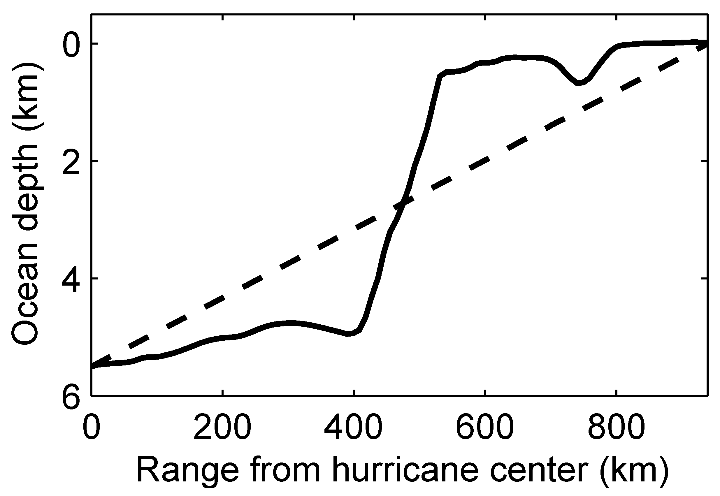
The ocean depth (solid line) between hurricane Bonnie and the seismometer in Florida at noon on 24 August. Also shown is the ocean depth for the idealized up-sloping environment used to calculate the Green functions in Section 3 (dashed line). The scale of the figure makes the actual slope appear to change rapidly; however, the maximum slope of the ocean floor is roughly .
Figure 4.
The ocean depth (solid line) between hurricane Bonnie and the seismometer in Florida at noon on 24 August. Also shown is the ocean depth for the idealized up-sloping environment used to calculate the Green functions in Section 3 (dashed line). The scale of the figure makes the actual slope appear to change rapidly; however, the maximum slope of the ocean floor is roughly .

Figure 5.
Horizontal (a–d) and vertical (e–h) velocity spectra modeled (red dashed) and measured (blue) at the seismometer in Florida at four times on 24 August 1998. The dotted blue lines represent portions of the data that where dominated by non-hurricane related ambient noise. Note that the peak in the spectra is at roughly Hz. This frequency corresponds to the peak in the wave height spectrum at rad/m seen in Figure 2.


Table 1.
Parameters for Hurricane Bonnie on 24 August 1998.
| Time | Hurricane Center Position | Range from | Ocean Depth at | |
|---|---|---|---|---|
| Lat (N) | Lon (W) | Sensor (km) | Hurricane Center (km) | |
| 0000 | 24.8 | 71.8 | 1028 | 5.1 |
| 0600 | 25.2 | 72.1 | 983 | 5.5 |
| 1200 | 25.6 | 72.4 | 939 | 5.5 |
| 1800 | 26.1 | 72.8 | 881 | 5.2 |
© 2018 by the author. Licensee MDPI, Basel, Switzerland. This article is an open access article distributed under the terms and conditions of the Creative Commons Attribution (CC BY) license (http://creativecommons.org/licenses/by/4.0/).
Share and Cite
MDPI and ACS Style
Wilson, J.D. Modeling Microseism Generation by Inhomogeneous Ocean Surface Waves in Hurricane Bonnie Using the Non-Linear Wave Equation. Remote Sens. 2018, 10, 1624. https://doi.org/10.3390/rs10101624
AMA Style
Wilson JD. Modeling Microseism Generation by Inhomogeneous Ocean Surface Waves in Hurricane Bonnie Using the Non-Linear Wave Equation. Remote Sensing. 2018; 10(10):1624. https://doi.org/10.3390/rs10101624
Chicago/Turabian StyleWilson, Joshua D. 2018. "Modeling Microseism Generation by Inhomogeneous Ocean Surface Waves in Hurricane Bonnie Using the Non-Linear Wave Equation" Remote Sensing 10, no. 10: 1624. https://doi.org/10.3390/rs10101624
Note that from the first issue of 2016, this journal uses article numbers instead of page numbers. See further details here.