Unsupervised Feature Selection Based on Ultrametricity and Sparse Training Data: A Case Study for the Classification of High-Dimensional Hyperspectral Data

Abstract

In this paper, we investigate the potential of unsupervised feature selection techniques for classification tasks, where only sparse training data are available. This is motivated by the fact that unsupervised feature selection techniques combine the advantages of standard dimensionality reduction techniques (which only rely on the given feature vectors and not on the corresponding labels) and supervised feature selection techniques (which retain a subset of the original set of features). Thus, feature selection becomes independent of the given classification task and, consequently, a subset of generally versatile features is retained. We present different techniques relying on the topology of the given sparse training data. Thereby, the topology is described with an ultrametricity index. For the latter, we take into account the Murtagh Ultrametricity Index (MUI) which is defined on the basis of triangles within the given data and the Topological Ultrametricity Index (TUI) which is defined on the basis of a specific graph structure. In a case study addressing the classification of high-dimensional hyperspectral data based on sparse training data, we demonstrate the performance of the proposed unsupervised feature selection techniques in comparison to standard dimensionality reduction and supervised feature selection techniques on four commonly used benchmark datasets. The achieved classification results reveal that involving supervised feature selection techniques leads to similar classification results as involving unsupervised feature selection techniques, while the latter perform feature selection independently from the given classification task and thus deliver generally versatile features.

1. Introduction

The analysis of large geospatial data is a topic of major interest in the fields of photogrammetry and remote sensing. In many cases, such an analysis relies on a semantic classification which, in turn, typically associates high-dimensional feature vectors with semantic classes. To allow for an appropriate assignment, standard supervised classification techniques need to be trained with representative training data. Regarding geospatial data, the latter are however often hard to obtain and/or quite costly, so that only few training data might be available. An exemplary scenario is for instance given with the classification of hyperspectral imagery acquired via airborne or spaceborne platforms. Here, training data are generated by manually assigning respective ground truth labels to numerous pixels. For this purpose, expert knowledge (e.g., on the spectral behavior of land cover and land use classes across the spectral bands) is typically required. Involving expert knowledge, the manual annotation might strongly rely on visual differences in the image (considering several band combinations) and the individual spectra of respective pixels [1]. This becomes even more challenging if the number of considered classes is rather high and if very large amounts of training data need to be collected.

The semantic classification of high-dimensional feature vectors with only a few available and thus sparse training data is often addressed by introducing feature selection techniques. On the one hand, such techniques may exploit relations between features and classes which are estimated via measures of distance, information, dependence/correlation or consistency [2,3,4,5]. On the other hand, such techniques may interact with a classifier [3,6] and thus rely on an error rate measure [2] to find a set of suitable features via an exhaustive search over all conceivable feature combinations. The derived feature sets are thus optimized with respect to the involved classifier and possibly its internal settings, and they may therefore vary if different classifiers are used. Besides feature selection techniques, dimensionality reduction techniques can be applied. Such techniques focus on the transformation of the high-dimensional feature vectors to a new representation of lower dimensionality, e.g., via a linear transformation in case of a Principal Component Analysis (PCA). Due to the involved transformation, the new representation relies on meta-features, e.g., represented by the principal components in case of a PCA.

1.1. Contribution

In this paper, we aim to combine the main advantages of feature selection and dimensionality reduction techniques. On the one hand, we want to retain a suitable subset of the original features for the sake of interpretability. On the other hand, we want to use only intrinsic properties of the feature vectors given with the representative training data to select such features, while information about the corresponding labels should not be considered. We argue that the consideration of such labels would make the selection of features dependent on the considered classes and thus the considered classification task. Consequently, we focus on unsupervised feature selection relying on the topology of the given training data. More specifically, we investigate the degree to which the training data reveal an ultrametric behavior. Thereby, we use different ultrametricity indices exploiting either triangles within the given data or a specific graph structure. To demonstrate the potential of such unsupervised feature selection techniques, we exemplarily focus on the classification of high-dimensional hyperspectral data acquired via airborne or spaceborne platforms. In summary, the key contributions of this paper are:

• the presentation of an approach for unsupervised feature selection based on the topology of given sparse training data,
• the use of different ultrametricity indices to describe the topology of given training data,
• the in-depth analysis of the potential of the proposed approach for unsupervised feature selection for the classification of high-dimensional hyperspectral data, and
• the comparison of achieved results with those of state-of-the-art feature selection and dimensionality reduction techniques.

1.2. Paper Outline

After briefly summarizing related work in Section 1.3, we present our framework for classifying high-dimensional feature vectors with only sparse training data in Section 2. To demonstrate the performance of our framework, we focus on the classification of hyperspectral data, an exemplary scenario in which typically only sparse training data are available for the semantic classification of high-dimensional feature vectors. Using four benchmark datasets, we conduct an objective performance evaluation for different configurations of our framework in Section 3. The achieved results are discussed in detail in Section 4. Finally, we provide concluding remarks and suggestions for future work in Section 5.

1.3. Related Work

In the following, we briefly summarize related work. As our case study focuses on the classification of high-dimensional hyperspectral data, we first take a glance on feature extraction (Section 1.3.1) which delivers the high-dimensional data. However, it has been proven in practice that a large amount of considered features does not necessarily lead to the best possible classification results. For this reason, approaches focusing on dimensionality reduction or feature selection are typically involved (Section 1.3.2). Finally, we focus on related work with respect to classification (Section 1.3.3).

1.3.1. Feature Extraction

Due to the consideration of a general classification task, we consider a classification of single data points (here: pixels) without taking into account neighborhood relations among data points (here: relations within the pixel neighborhood). Accordingly, each pixel in the hyperspectral imagery is typically described by considering spectral features in the form of reflectance values across all spectral bands and concatenating them to a feature vector.

There are also approaches for the classification of hyperspectral imagery which focus on spatial features, where relations within the pixel neighborhood are taken into account. Such spatial features have for instance been presented with morphological profiles [7] or morphological attribute profiles [8,9]. Furthermore, it has been proposed to derive features by sampling spectral information within adaptive pixel neighborhoods [10] or to derive segment-based features from superpixels [11,12,13]. As spatial features allow describing local image features such as edges, corners and spots, it has also been proposed to efficiently extract texture information preserved in hyperspectral imagery by using local binary patterns and global Gabor filters in a set of selected bands [14]. In this regard, image features are described using a local neighborhood with a certain size. To take into account spatial image features at multiple scales, an extension towards the use of multiscale texture features has been presented [15]. Besides, it has been proposed to fuse information from adjacent spectral bands, e.g., by extracting texture features from different direction patterns and thereby not only considering neighboring pixels but also the characteristics across consecutive bands [16].

A variety of investigations also focuses on spectral unmixing [17,18,19,20]. There, the objective consists in decomposing the measured spectrum of each pixel into a collection of its constituent spectral signatures (“endmembers”) and a set of corresponding values (“abundances”) indicating the contribution of each spectral signature. Particularly regarding the classification of hyperspectral imagery, where pixels may correspond to a relatively large spatial size, it is likely to have several materials or substances that contribute to the respectively measured spectrum. To decompose the latter into spectral signatures corresponding to various materials or substances, both linear and non-linear (mostly geometrical or statistical) approaches for spectral unmixing have been proposed [17,18,19,20].

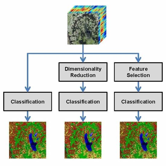
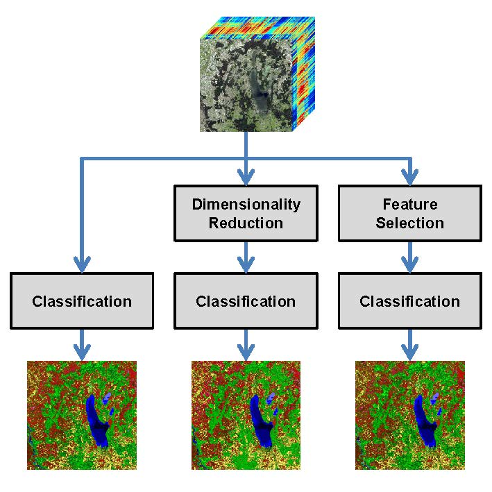
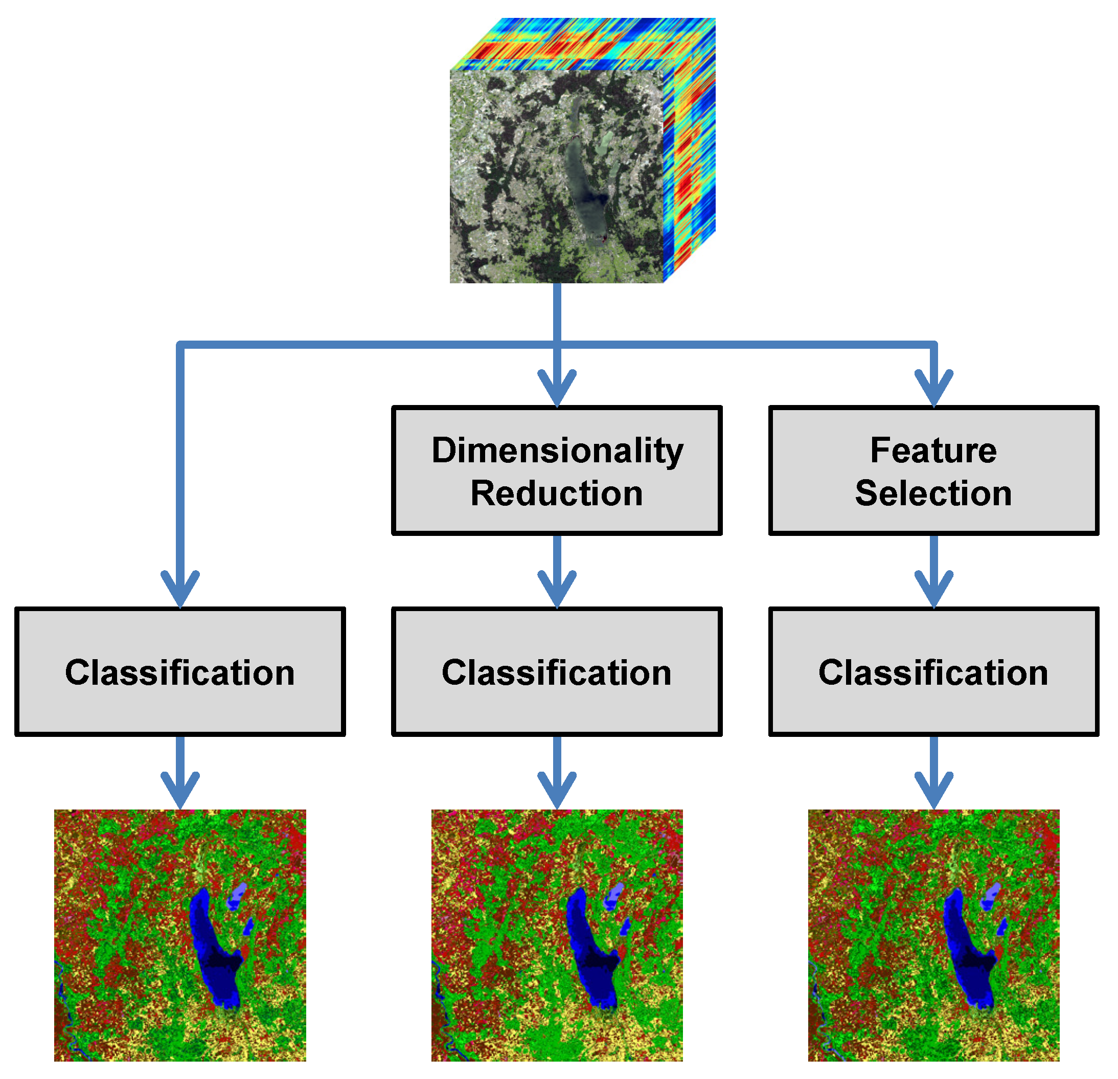
1.3.2. Dimensionality Reduction (DR) vs. Feature Selection (FS)

For many applications, as many features as possible are extracted in the hope to compensate a lack of knowledge about the scene and/or data. Among the extracted features, however, some might be more relevant, whereas others might be less relevant or even redundant. Particularly for the classification of high-dimensional data, one has to take into account the Hughes phenomenon [21]. According to this phenomenon, an increase of the number of features over a certain threshold decreases the predictive accuracy of a classifier, given a constant number of training examples. In the context of classifying hyperspectral data, the Hughes phenomenon has been reported in [22,23]. However, it has also been verified for classification tasks relying only on a relatively small number of features, e.g., in [24].

To address the Hughes phenomenon, several approaches focus on dimensionality reduction where the objective is to derive a new data representation based on fewer, but potentially better features extracted from the given data representation. In this regard, the most commonly applied techniques are represented by variants of Principal Component Analysis (PCA) [25], Independent Component Analysis (ICA) [26,27], or Linear Discriminant Analysis (LDA) [28]. These techniques apply linear transformations to map the given feature space (which is spanned by the complete set of hyperspectral bands in our case) to a new space spanned by meta-features. Using such techniques, certain characteristics of the considered data are contained in very few meta-features which are used as the basis for subsequent tasks. While this typically improves both effectiveness and efficiency, derived results hardly allow concluding about relationships with respect to physical properties (as e.g., possible when considering the wavelengths of involved spectral bands).

Consequently, another strategy to address the Hughes phenomenon is followed by feature selection. Here, the objective is to retain the most relevant and most informative features among a set of features, i.e., a subset of the original features, while discarding less relevant and/or redundant features. This, in turn, typically allows gaining predictive accuracy, improving computational efficiency with respect to both time and memory consumption, and retaining meaningful features with respect to the given task [3,6]. In general, one may distinguish between supervised and unsupervised feature selection techniques. The supervised techniques can further be sub-categorized into three groups:

• Filter-based methods focus on evaluating relatively simple relations between features and classes and possibly also among features. These relations are typically quantified via a score function which is directly applied to the given training data [4,6,24,29]. Such a classifier-independent scheme typically results in simplicity and efficiency. Many respective methods only focus on relations between features and classes (univariate filter-based feature selection). These relations can be quantified by comparing the values of a feature across all data points with the respective class labels, e.g., via the correlation coefficient [30], Gini index [31], Fisher score [32], or information gain [33]. This allows ranking the features with respect to their relevance. Other methods take into account both feature-class relations and feature-feature relations (multivariate filter-based feature selection) and can thus be used to remove redundancy to a certain degree. Respective examples are represented by Correlation-based Feature Selection [34] and the Fast Correlation-Based Filter [35].
• Wrapper-based methods rely on the use of a classifier in order to select features based on their suitability for classification. On the one hand, this may be achieved via Sequential Forward Selection (SFS) where, beginning with an empty feature subset, it is tested which feature can be added so that the increase in performance is as high as possible. Accordingly, classification is first performed separately for each available feature. The feature leading to the highest predictive accuracy is then added to the feature subset. The following steps consist in successively adding the feature that improves performance the most when considering the existing feature subset and the tested feature as input for classification. On the other hand, a classifier may be involved via Sequential Backward Elimination (SBE) where, beginning with the whole feature set, it is tested which feature can be discarded so that the decrease in performance is as low as possible. The following steps consist in successively removing the feature that reduces performance the least. Besides sequential selection, genetic algorithms which represent a family of stochastic optimization heuristics can be involved to select feature subsets [36].
• Embedded methods rely on the use of a classifier which provides the capability to internally select the most relevant features during the training phase of the classifier. Prominent examples in this regard are represented by the AdaBoost classifier [37] and the Random Forest classifier [38]. In contrast to wrapper-based methods, the involved classifier has to be trained only once to be able to conclude about the relevance of single features and the computational effort is therefore still acceptable, particularly for the Random Forest classifier which reveals a reasonable computational effort for both training and testing phase.

For more details, we refer to a comprehensive review of feature selection techniques [3]. Note that many of these techniques require training data with a balanced number of training examples per class as otherwise a bias in feature selection can be expected. From our brief summary, however, it becomes obvious that, particularly for high-dimensional data as given for hyperspectral imagery, applying a wrapper-based method can be extremely time-consuming. For this reason, we do not involve respective techniques in the scope of this paper.

As supervised feature selection via a wrapper-based method or an embedded method relies on the use of a classifier, the selected feature sets strongly depend on the involved classifier and its settings. Furthermore, the feature sets are selected with respect to a particular classification task and therefore depend on the number as well as on the definition of the considered classes. The latter also holds for filter-based methods evaluating relations between features and classes. To avoid such dependencies and hence make feature selection independent of the classifier as well as of the classification task, it seems desirable to conduct unsupervised feature selection which however typically implies an increased computational burden.

Among the unsupervised feature selection techniques, the main objective is represented by a clustering of the input data. In analogy to supervised feature selection, a categorization with respect to filter-based and wrapper-based methods can also be applied for unsupervised feature selection [39,40]. In the context of unsupervised feature selection, wrapper-based methods rely on the idea of first applying a clustering algorithm and then evaluating the quality of the derived clustering via cluster validation techniques [41]. During this process, no external information in the form of corresponding class labels is involved. It has been found that a dynamic number of allowed clusters is to be preferred [42]. Regarding unsupervised feature selection, relevant features are often selected based on the distribution of their values across the given feature vectors, e.g., by using an entropy measure which allows reasoning about the existence and the significance level of clusters [43]. A different strategy for unsupervised feature selection relies on assessing the similarity between features and selecting a subset of features that are highly dissimilar from each other [44,45,46,47], whereby different similarity metrics can be used. Furthermore, the BandClust algorithm [48] has been proposed which relies on a minimization of mutual information to split the given range of spectral bands into disjoint clusters or sub-bands. A probabilistic model-based clustering approach has been presented in [49]. Thereby, the parameters of the model are inferred by maximizing the information between data features and cluster assignments. Besides such clustering techniques, the Random Cluster Ensemble (RCE) technique [50] relies on the variable importance measure used in Random Forests and estimates the out-of-bag feature importance from an ensemble of partitions. Moreover, unsupervised feature selection based on a self-organizing map (SOM) [51] has been proposed for the analysis of high-dimensional data [52] and for a case study focusing on the analysis of near-infrared data in terms of a prediction of certain properties of biodiesel fuel [53]. For a performance evaluation of different unsupervised feature selection methods in the context of analyzing hyperspectral data, we refer to [47,54].

A summary of the main characteristics of the different concepts for dimensionality reduction and feature selection is provided in

Table 1. Categorization of feature selection (FS) techniques with respect to their main characteristics: the table follows [3] and additionally addresses unsupervised FS techniques (SFS: Sequential Forward Selection; SBE: Sequential Backward Elimination; CFS: Correlation-based Feature Selection; FCBF: Fast Correlation-Based Filter; MUI: Murtagh Ultrametricity Index; TUI: Topological Ultrametricity Index; BOFR: Baire-Optimal Feature Ranking). Note that all FS techniques retain a subset of the original features, whereas dimensionality reduction techniques transform the original data into a new feature space of lower dimensionality where dimensions do not correspond to the original features.

Category	Strategy	Characteristics	Examples
Supervised	Filter-based FS
	-Univariate	+ Simple	Fisher score
		+ Fast	Information gain
		+ Classifier-independent selection	Symm. uncertainty
		− No feature dependencies
		− No interaction with the classifier
	-Multivariate	+ Classifier-independent selection	CFS [34]
		+ Models feature dependencies	FCBF [35]
		+ Faster than wrapper-based FS
		− Slower than univariate techniques
		− No interaction with the classifier
	Wrapper-based FS	+ Interaction with the classifier	SFS
		+ Models feature dependencies	SBE
		− Classifier-dependent selection
		− Computationally intensive
		− Risk of over-fitting
	Embedded FS	+ Interaction with the classifier	Random Forest
		+ Models feature dependencies	AdaBoost
		+ Faster than wrapper-based FS
		− Classifier-dependent selection
Unsupervised	Filter-based FS	+ Classifier-independent selection	Clustering
		+ Models feature dependencies	MUI (proposed)
		− No interaction with the classifier	TUI (proposed)
			BOFR (proposed)
	Wrapper-based FS	+ Classifier-independent selection	Cluster validation
		+ Models feature dependencies
		− Computationally intensive

.

In this paper, we propose to perform feature selection without taking into account the classification task, i.e., the class labels of the considered data. Accordingly, we focus on unsupervised feature selection only taking into account the characteristics of features which are implicitly preserved in the topology of the given data. To describe these characteristics, we consider the ultrametricity in the data. An important motivation for finding ultrametricity in data is that nearest neighbor search can be carried out very efficiently [55]. In general, an “ultrametric” is a distance d which satisfies the strict triangle inequality:

$$d(x,y)\le max\left\{d(x,z),d(z,y)\right\}$$

(1)

with x, y and z referring to data points. After a p-adic encoding of data, ultrametric spaces have simpler classification algorithms than their classical counterparts [56,57]. This motivates to measure the ultrametricity of very high-dimensional data [58], and it has been found that they are increasingly ultrametric as their dimension increases. Accordingly, it becomes increasingly easy to find clusters, as the high-dimensional structure is hierarchical in the limit. The results presented in [58] lead to believe that high-dimensional encoding of data reveals the inherent ultrametric, i.e., hierarchical, structure of data, rather than imposing such on data. In this way, an ultrametric or almost ultrametric encoding of data should lead to better classification results than other data encodings. Thus measures for the ultrametricity of data become crucial.

There are different ways of measuring the ultrametricity of data taken from a metric space such as ${\mathbb{R}}^D$. The first such method has been introduced in [59] and considers the discrepancy between the given metric d and its subdominant ultrametric which is the unique maximal ultrametric below d [60]. It has the problem that it is biased towards the single-link clustering. In this hierarchical clustering method, the similarity of two clusters is the similarity of their most similar elements. This makes single-link clustering suffer from the undesired chaining effect where clusters become almost linear arrangements of points. In order to remedy this effect, Murtagh defines an ultrametricity index which overcomes the chaining effect as the ratio between the number of triangles which are almost isosceles and the number of all triangles in the data [55]. Furthermore, a clustering based on ultrametric properties is described in [61].

1.3.3. Classification

The derived feature vectors serve as input for classification. For classifying hyperspectral imagery, the classic approach consists in a pixel-wise classification, e.g., by using widely used standard classifiers such as a Support Vector Machine (SVM) or a Random Forest (RF) classifier [1,22,23,62]. These approaches often yield reasonable classification results, but—due to classifying each pixel individually by only considering the corresponding feature vector—it is not taken into account that the labels of neighboring pixels tend to be correlated.

To account for spatial context in classification and thus conduct spectral-spatial classification, different strategies have been followed. Relying on the results of a pixel-wise classification, it has for instance been proposed to apply a majority voting within watershed segments to achieve a spectral-spatial classification [63]. Furthermore, approaches for spectral-spatial classification have been presented which consist in a probabilistic SVM-based pixel-wise classification followed by a Markov Random Field (MRF) regularization [64] or a hierarchical optimization [65]. A different context model has been used by involving a Conditional Random Field [11] for spectral-spatial classification. Recently, the use of deep learning techniques for spectral-spatial classification of hyperspectral imagery has been paid increased attention to. In [66], for instance, a Convolutional Neural Network (CNN) is used which consists of several convolutional layers and pooling layers which allow the extraction of deep spectral-spatial features that are highly discriminant. While the use of such deep features significantly improves the classification results, a CNN involves a huge number of parameters that have to be tuned during the training process. In case of labeled hyperspectral imagery, however, only a rather limited amount of training data is typically available.

A different avenue of research on the classification of hyperspectral imagery focused on the fact that manual annotation in terms of labeling single pixels typically contains highly redundant information for the classification task. Furthermore, due to noise effects, class statistics might not appropriately be represented which in turn results in a decrease of the predictive accuracy of the involved classifier. Accordingly, some investigations focused on selecting training data in a smart way so that a small training set of highly discriminative examples is sufficient to appropriately represent the class boundaries and conduct classification for new examples. In this regard, a popular strategy is followed by Active Learning (AL) [67,68] where the main idea consists in training a classifier on a small set of training examples that are well-chosen via an interaction between the user and the classifier. More specifically, the classifier is first trained on a small, but non-optimal set of training examples. The classification of further examples reveals the examples for which the classification result is quite uncertain. For the most uncertain predictions, the user assigns the correct labels so that the respective examples can be included in the training set for reinforcement learning. Thus, the classifier is optimized on well-chosen difficult training examples, and improved generalization capabilities can therefore be expected.

2. Materials and Methods

In the scope of this paper, we consider the workflow of a standard classification task based on high-dimensional input data, but we assume that only sparse training data are available. For this reason, we focus on a case study for the classification of hyperspectral data, in which such a scenario might be given and for which several benchmark datasets are available (Section 2.1). Despite a feature extraction tailored to hyperspectral data (Section 2.2), the other parts of our proposed methodology which are represented by dimensionality reduction/feature selection (Section 2.3) and classification (Section 2.4) can generally be applied for very different types of data. An overview on our framework is given in Figure 1. In the following, we briefly outline the involved methods and provide more detailed explanations on the proposed contributions relying on unsupervised feature selection.

2.1. Datasets

For our experiments, we use four benchmark datasets which are commonly used for evaluating approaches focusing on the classification of hyperspectral data. Three of these benchmark datasets (Section 2.1.1, Section 2.1.2 and Section 2.1.3) are publicly available in a repository of hyperspectral remote-sensing scenes (http://www.ehu.eus/ccwintco/index.php?title=Hyperspectral_Remote_Sensing_Scenes). The fourth benchmark dataset (Section 2.1.4) consists of simulated Environmental Mapping and Analysis Program (EnMAP)-like data.

2.1.1. Pavia Centre

The Pavia Centre dataset has been acquired with the Reflective Optics System Imaging Spectrometer (ROSIS) [69] in a low-altitude flight campaign over the city of Pavia which is located in the northern part of Italy. The considered scene represents an urban area, and it is sampled as two images of $1096\times 223$ pixels and $1096\times 492$ pixels, respectively. Each pixel corresponds to an area of $1.3$ m ×$1.3$ m. For each pixel, information on 102 spectral bands is available. In total, the dataset consists of more than 783 k pixels of which $7456$ have been labeled with respect to 9 classes as shown in Figure 2 (left), while no reference labels are provided for the remaining pixels.

2.1.2. Pavia University

The Pavia University dataset has also been acquired with the Reflective Optics System Imaging Spectrometer (ROSIS) [69] over the city of Pavia, Italy. The considered scene represents an urban area, and it is sampled as an image of $610\times 340$ pixels, where each pixel corresponds to an area of $1.3$ m × $1.3$ m. For each pixel, information on 103 spectral bands is available. In total, the dataset consists of more than 207 k pixels of which $42,776$ have been labeled with respect to 9 classes as shown in Figure 2 (right), while no reference labels are provided for the remaining pixels.

2.1.3. Salinas

The Salinas dataset has been acquired with the Airborne Visible/Infrared Imaging Spectrometer (AVIRIS) (http://aviris.jpl.nasa.gov) in a low-altitude flight campaign over Salinas Valley which represents one of the major valleys and most productive agricultural regions in California, USA. The considered scene is mainly characterized by vegetables, corn, bare soils and vineyards, and it is represented as an image of $512\times 217$ pixels, where each pixel corresponds to an area of $3.7$ m × $3.7$ m. For each pixel, information on 224 spectral bands has been acquired with the AVIRIS sensor; yet 20 water absorption bands have been removed so that only information on 204 spectral bands is available for our experiments. In total, the dataset consists of more than 111 k pixels of which 54,129 have been labeled with respect to 16 classes as shown in Figure 3, while no reference labels are provided for the remaining pixels.

2.1.4. EnMAP

The EnMAP dataset has been derived from the simulated EnMAP Alpine Foothills dataset [70,71] and contains an additional labeling with respect to different land use classes [1]. The main aim of the original dataset consists in providing hyperspectral data as it would be acquired with a future hyperspectral satellite mission represented by the EnMAP mission. The considered scene is characterized by a rich diversity of water, vegetation, agricultural, and urban/industrial classes and it corresponds to an area of about 30 km × 30 km around the Ammersee in Bavaria, Germany. This area is represented as an image of $1000\times 1000$ pixels, where each pixel thus corresponds to an area of 30 m × 30 m. For each pixel, information on 244 simulated spectral bands is available. In total, the dataset consists of 1 M pixels of which $3741$ have been labeled with respect to 20 classes as shown in Figure 4, while no reference labels are provided for the remaining pixels. The labeled pixels are separated in a training set containing $2617$ labeled pixels and a test set comprising $1124$ labeled pixels.

2.2. Feature Extraction

Our main contribution addresses the selection of relevant features from a given set of features for very different types of data. For this reason, we do neither focus on spatial-spectral considerations [72] nor on techniques of spectral unmixing [17,18,19], which are often used for processing hyperspectral data, but cannot be used without significant adaptations for other types of data (e.g., laser scanning data) or different classification tasks (e.g., tree species classification from laser scanning data). Hence, we consider only the spectral information preserved in the form of reflectance values across a large number of spectral bands in the scope of this paper. Consequently, each pixel is characterized by a feature vector resulting from the concatenation of the respective reflectance values across the spectral bands.

For all subsequent parts, the following notation is used: we denote the combination of all data derived via feature extraction by a matrix $\mathbf{f}\in {\mathbb{R}}^{N\times D}$. The matrix $\mathbf{f}$ contains a set of N feature vectors ${\mathbf{f}}_{i,*}$ with $i=1,\cdots ,N$ that are represented by the rows of $\mathbf{f}$. Each feature vector ${\mathbf{f}}_{i,*}\in {\mathbb{R}}^{1\times D}$ is given in a D-dimensional space spanned by the features $f_j$ with $j=1,\cdots ,D$. Using this notation, a feature $f_j$ is represented by a single value per pixel (here: the reflectance value of a specific spectral band). In addition, we may also consider the behavior of single features $f_j$ across all feature vectors ${\mathbf{f}}_{i,*}$. For this purpose, we consider the concatenation of the values of a feature $f_j$ across all feature vectors ${\mathbf{f}}_{i,*}$. This concatenation is represented by a column vector ${\mathbf{f}}_{*,j}\in {\mathbb{R}}^{N\times 1}$.

2.3. Dimensionality Reduction (DR) vs. Feature Selection (FS)

To address the Hughes phenomenon [21], we involve methods for both dimensionality reduction (DR) and feature selection (FS). For the latter, we consider commonly used supervised methods and our proposed unsupervised methods.

2.3.1. DR: Principal Component Analysis (PCA)

For dimensionality reduction, we use a standard Principal Component Analysis (PCA). This choice is motivated by the fact that the PCA is still the most commonly applied technique for dimensionality reduction. The PCA transforms the given feature space (here: the feature space spanned by all hyperspectral bands) to a new feature space spanned by linearly uncorrelated meta-features. These are the principal components, which describe the variability of the given data along the respective dimension. Accordingly, the most relevant information is preserved in those meta-features indicating the highest variability.

For PCA-based feature ranking, we sort the meta-features with respect to the variability of the given data covered by them. For PCA-based feature subset selection, we use the set of most relevant meta-features which covers $99.9$% of the variability of the given data, and we expect there to be no significant loss of relevant information when using only these few meta-features.

2.3.2. Supervised FS: Random Forest’s Mean Decrease in Permutation Accuracy (RF-MDPA)

The Random Forest (RF) classifier [38] can be used as an embedded method for supervised filter-based feature selection. More specifically, it allows ranking features with respect to a feature importance measure represented by the mean decrease in permutation accuracy (MDPA). Following [73], the main idea consists in training each tree on a randomly chosen subset of the training data, i.e., a bootstrap sample, and then performing the prediction for the data which are not in the bootstrap sample, i.e., the out-of-bag (OOB) data. Subsequently, the OOB predictions of all trees are aggregated and an error rate is derived. To estimate the importance of a variable, it is tested how much the prediction error increases if OOB data for that variable are randomly permuted.

2.3.3. Supervised FS: A General Relevance Metric (GRM)

To select a compact and robust subset comprising relevant and informative features, a filter-based FS method relying on a general relevance metric (GRM) has recently been proposed [24]. The main idea of this method consists in addressing different intrinsic properties of the given training data for feature relevance assessment. This is achieved via the integration of seven different metrics for ranking features according to their relevance: the Pearson correlation coefficient [30], the Fisher score [32], the Gini index [31], the information gain [33], the ReliefF measure [74] and two measures derived from a ${\chi }^2$-test and a t-test. For each relevance metric, a feature ranking is performed separately. Subsequently, the mean rank of each feature across all separate rankings is taken into consideration to distinguish between more and less relevant features. For more details, we refer to [24] and references therein.

2.3.4. Supervised FS: Correlation-Based Feature Selection (CFS)

The Correlation-based Feature Selection (CFS) [34] aims at multivariate filter-based feature selection, i.e., it relies on a score function evaluating feature-class relations as well as feature-feature relations in order to discriminate between relevant, irrelevant and redundant features. In the following, we consider a set of features $f_j$ (i.e., the spectral bands in our case), the concatenation of the respective values across all considered data points to a vector ${\mathbf{f}}_{*,j}$ and the corresponding label vector $\mathbf{c}$. Using this notation, the CFS method relies on a correlation metric represented by the symmetrical uncertainty $SU$ [75]. Accordingly, the correlation between a feature $f_j$ and the label vector $\mathbf{c}$ results in

$$SU({\mathbf{f}}_{*,j},\mathbf{c})=2\frac{E\left({\mathbf{f}}_{*,j}\right)+E\left(\mathbf{c}\right)-E\left({\mathbf{f}}_{*,j}\right|\mathbf{c})}{E\left({\mathbf{f}}_{*,j}\right)+E\left(\mathbf{c}\right)}=2\frac{MI({\mathbf{f}}_{*,j},\mathbf{c})}{E\left({\mathbf{f}}_{*,j}\right)+E\left(\mathbf{c}\right)}$$

(2)

where $E(·)$ represents the entropy and $MI(·,·)$ represents the mutual information. Furthermore, the correlation between a feature $f_{j1}$ and a feature $f_{j2}$ is given by

$$SU({\mathbf{f}}_{*,j1},{\mathbf{f}}_{*,j2})=2\frac{E\left({\mathbf{f}}_{*,j1}\right)+E\left({\mathbf{f}}_{*,j2}\right)-E\left({\mathbf{f}}_{*,j1}\right|{\mathbf{f}}_{*,j2})}{E\left({\mathbf{f}}_{*,j1}\right)+E\left({\mathbf{f}}_{*,j2}\right)}=2\frac{MI({\mathbf{f}}_{*,j1},{\mathbf{f}}_{*,j2})}{E\left({\mathbf{f}}_{*,j1}\right)+E\left({\mathbf{f}}_{*,j2}\right)}$$

(3)

respectively. Denoting the average correlation between features and classes as ${\overline{\rho }}_{fc}$ and the average correlation between different features as ${\overline{\rho }}_{ff}$, the relevance R of a feature subset comprising $N_f$ features can be evaluated:

$$R(f_{1\cdots N_f},c)=\frac{N_f{\overline{\rho }}_{fc}}{\sqrt{N_f+N_f(N_f-1){\overline{\rho }}_{ff}}}$$

(4)

Obtaining a suitable feature subset thus corresponds to maximizing the relevance R by searching the feature subset space [34]. This is done via an iterative scheme where, in each iteration, either a feature is added to the feature subset (forward selection) or a feature is removed from the feature subset (backward elimination) until the relevance R converges to a stable value.

2.3.5. Supervised FS: Fast Correlation-Based Filter (FCBF)

The Fast Correlation-Based Filter (FCBF) [35] exploits the symmetrical uncertainty $SU({\mathbf{f}}_{*,j1},\mathbf{c})$ as correlation metric in order to rank the features $f_{j1}$ (i.e., the spectral bands in our case) with respect to their correlation to the label vector $\mathbf{c}$. To decide whether a feature is relevant or not, heuristics are involved in terms of defining a certain threshold above which the symmetrical uncertainty indicates a relevant feature, i.e., $SU({\mathbf{f}}_{*,j1},\mathbf{c})>\delta$. In addition, the FCBF method aims at removing redundant features by comparing the symmetrical uncertainty $SU({\mathbf{f}}_{*,j1},{\mathbf{f}}_{*,j2})$ among features to the symmetrical uncertainty $SU({\mathbf{f}}_{*,j1},\mathbf{c})$ between features and classes. As a consequence, only the predominant features $f_{j1}$ are kept which satisfy the constraint $SU({\mathbf{f}}_{*,j1},\mathbf{c})>SU({\mathbf{f}}_{*,j1},{\mathbf{f}}_{*,j2})$ for all other features $f_{j2}$.

2.3.6. Unsupervised FS: Murtagh Ultrametricity Index (MUI)

For unsupervised feature selection, we consider the topology of the given data. More specifically, we focus on describing the degree to which the data reveal an ultrametric behavior. A respective approach has been presented in [55], where Murtagh introduces an ultrametricity index. This index is defined as the ratio between all almost isosceles triangles with short base and all triangles within the given data. Thereby, “almost” isosceles means that the difference between the two largest angles in a triangle is at most 2 degrees. We call such triangles “almost ultrametric”, and we use them to define the Murtagh Ultrametricity Index (MUI) $m\left(X\right)$ for data points $X\subset {\mathbb{R}}^D$ (here: a set of feature vectors ${\mathbf{f}}_{i,*}$):

$$m\left(X\right)=\frac{\#\mathrm{almost}\mathrm{ultrametric}\mathrm{triangles}\mathrm{in}X}{\#\mathrm{all}\mathrm{triangles}\mathrm{in}X}$$

(5)

The reason for defining this index in such a way is that, in an ultrametric space, all triangles are isosceles with small base. This ultrametricity index does not suffer from the chaining effect (which is given if a cluster has a small spread in one direction and a larger spread in another direction), unlike the method derived by Rammal in [59]. Murtagh finds that very high-dimensional data tend to be increasingly ultrametric, and it becomes easier to find clusters in high dimensions [58].

To apply the MUI for unsupervised feature selection, we follow the strategy of an SFS scheme. Consequently, we start with a minimal set of features (here: a set of two features, i.e., two spectral bands, since triangles are not defined when considering only a single feature) and successively add the most suitable one of the remaining features until all features have been added. This results in a feature ranking. More specifically, we first evaluate the MUI for all conceivable combinations of two features by considering the respectively defined data points. The set of two features corresponding to the highest MUI is then selected. Subsequently, all possible extensions of this set by one further feature are evaluated, and the feature that increases the MUI the most is added. This procedure is repeated until all features have been added and, thus, a ranking of the features can be derived.

To apply the MUI for unsupervised feature subset selection, the MUI itself can be considered for each repetition. For the first repetitions, we may assume that the MUI increases from step to step. However, at a certain step, the MUI might be decreasing again. We consider the latter case as a stopping criterion which allows us to automatically derive feature subsets comprising the few best-ranked features in an unsupervised manner. In addition, we consider the subset of best-ranked features yielding the global maximum of the MUI.

2.3.7. Unsupervised FS: Topological Ultrametricity Index (TUI)

We propose to address the topology of the given data with a different ultrametricity index which relies on a graph structure. More specifically, we represent the data $X\subset {\mathbb{R}}^D$ (here: the set of feature vectors ${\mathbf{f}}_{i,*}$) as a Vietoris-Rips graph. In general, a Vietoris-Rips graph ${\Gamma }_{ϵ}$ for $ϵ>0$ associated with some data X inside the Euclidean space ${\mathbb{R}}^D$ is given as:

• The vertex set is X.
• A pair of data points $(x,y)\in X\times X$ is an edge if and only if $d(x,y)\le ϵ$.

This graph is in fact the 1-skeleton of the Vietoris-Rips complex used in topological data analysis [76,77], and a fast construction of it for general metric spaces has been introduced in [78]. The Euclidean metric of ${\mathbb{R}}^D$ induces a metric d on the finite dataset X. From the point of view of classification, an ideal property of d is it being “ultrametric” which means that the strict triangle inequality

$$d(x,y)\le max\left\{d(x,z),d(z,y)\right\}$$

(6)

holds true. The reason is that, in this case, the hierarchical classification tree (i.e., the dendrogram) of X is unique. Then, any hierarchical classification algorithm exposes this inherent hierarchy. There is a characterization of the ultrametric property of the induced metric d in terms of the Vietoris-Rips graphs. Namely, d is an ultrametric if and only if for all $ϵ>0$ the connected components of the Vietoris-Rips graph ${\Gamma }_{ϵ}$ are cliques [79]. Hence, we consider for a graph $\Gamma$ the quantity

$$0<\mu (\Gamma ):=\frac{b_0(\Gamma )}{c(\Gamma )}\le 1$$

(7)

where $b_0(\Gamma )$ is the number of connected components and $c(\Gamma )$ is the number of maximal cliques in $\Gamma$. This quantity $\mu$ can be viewed as a measure of how many ultrametric balls (maximal cliques) the clusters (connected components) are made up. Relying on $\mu (\Gamma )$, we define the Topological Ultrametricity Index (TUI) as:

$$t(X,d):=\frac{1}{M}\underset{0}{\overset{M}{\int }}\mu \left(ϵ\right)dϵ$$

(8)

where M is the diameter of the metric space $(X,d)$, and $\mu \left(ϵ\right):=\mu \left({\Gamma }_{ϵ}\right)$. $t(X,d)$ is scale-invariant [79] and lies in the interval $(0,1]$. Here, $t(X,d)=1$ is equivalent to d having the ultrametric property. Hence, $t(X,d)$ measures how far a given metric is from ultrametric by determining how far from complete the connected components of ${\Gamma }_{ϵ}$ are.

Computing the TUI has a high time-complexity, because of the high cost for computing $c\left({\Gamma }_{ϵ}\right)$ when the graph ${\Gamma }_{ϵ}$ has many edges. There are in fact graphs $\Gamma$ with n vertices, for which $c(\Gamma )$ equals $3^{\frac{n}{3}}$ [80]. A way of overcoming this high time-complexity is explained in [81] as follows: Let $d_0<\cdots <d_n$ be the different positive values which the distance function d takes. Then, as $\mu \left(ϵ\right)$ is piece-wise constant,

$$t(X,d)=\frac{d_0}{d_n}+\frac{1}{d_n}\sum _{i=0}^{n-1}\mu \left(d_i\right)(d_{i+1}-d_i).$$

(9)

Hence, for $m<n$ we can define the truncation

$$t_m(X,d):=\frac{d_0}{d_n}+\frac{1}{d_n}\sum _{i=0}^{m-1}\mu \left(d_i\right)(d_{i+1}-d_i)$$

(10)

and compute it, instead of $t(X,d)$, for m such that the result is obtained in reasonable time.

One observes that the number of connected components in the Vietoris-Rips graph ${\Gamma }_{ϵ}$ decreases with increasing $ϵ$. In addition, the number of maximal cliques can be expected to increase with $ϵ$, except when $ϵ$ is near the maximal distance $d_n$. It follows that the contribution $\mu \left({\Gamma }_{ϵ}\right)$ is likely to be almost negligible for large values of $ϵ<d_n$. To reduce time-complexity, we hence define a stopping criterion relying on the slope to be smaller than some threshold $\xi >0$:

$$\frac{t_{m+1}-t_m}{\frac{d_{m+1}}{d_n}-\frac{d_m}{d_n}}=\mu \left({\Gamma }_{d_m}\right)\le \xi$$

(11)

where normalized distance values are used due to scale-invariance [81].

In [81], it is observed that $\mu \left(ϵ\right)$ looks like a continuous curve consisting of a part falling to almost zero, and then after some time rising back to 1. Furthermore, the falling part looks like the survival curve of a Weibull distribution. This allows to interpret the truncated topological ultrametricity index as the expected lifetime of an initially ultrametric dataset. In any case, it is this falling part which is captured by setting a threshold for the value of $\mu$ and then truncating the index t at this threshold.

In analogy to the MUI, the TUI can be applied for unsupervised feature selection with an SFS scheme. Consequently, we derive a feature ranking by starting with a minimal set of features (here: a minimal set comprising one single feature) and successively adding the most suitable one of the remaining features until all features have been added. More specifically, we first evaluate the TUI for all features separately by considering the respectively defined data points. The feature corresponding to the highest TUI is then selected as initial feature set. Subsequently, all possible extensions of this set by one further feature are evaluated, and the feature that increases the TUI the most is added. This procedure is repeated until all features have been added.

To apply the TUI for unsupervised feature subset selection, the TUI itself can be considered for each repetition. For the first repetitions, we may assume that the TUI increases from step to step. However, at a certain step, the TUI might be decreasing again. We consider the latter case as a stopping criterion which allows us to automatically derive feature subsets comprising the few best-ranked features in an unsupervised manner. In addition, we consider the subset of best-ranked features yielding the global maximum of the TUI.

2.3.8. Unsupervised FS: Baire-Optimal Feature Ranking (BOFR)

Another option for unsupervised feature selection is represented by Baire-Optimal Feature Ranking (BOFR). To successfully apply this approach, a certain discretization via rounding is required to derive feature vectors with partially identical entries from the given data points (here: a set of feature vectors ${\mathbf{f}}_{i,*}$ whose entries correspond to reflectance values at specific spectral bands) which consist of real-valued numbers. Then, for two data points x and y, the Baire distance can be defined as

$$d_{\mathrm{Baire}}(x,y)={\gamma }^{-\ell (x,y)}$$

(12)

with $\gamma >1$, where $\ell (x,y)$ is the length of the longest common prefix of x and y. The Baire distance is an ultrametric and is used in hierarchical classification [82]. An ordering of features (here: an ordering of the spectral bands, e.g., with respect to their corresponding wavelengths as commonly done) allows to view a data vector as an ordered sequence, and the Baire distance can be applied. However, in general, the ordering of features often relies on system-related or user-defined criteria, and there is for instance no natural ordering of features with respect to the topology of the given data, with respect to their contribution to the variability of considered data or with respect to their relevance for a classification task. To establish a suitable ordering via BOFR, orderings which minimize the mean Baire distance can be considered as proposed in [83]. It is shown there that for sufficiently small $\gamma >1$, this minimizing ordering can be found via gradient descent. In fact, each subset I of the total feature set induces a projection of the data by identifying any two data points $x,y$ whose feature vectors $x_I,y_I$ restricted to I coincide. The gradient descent adds a new feature j to I if the projection to $I\cup \left\{j\right\}$ has minimal number of elements among the projections to feature sets $I\cup \left\{k\right\}$. The time-complexity of this algorithm is shown to be $O\left(N^2{D}^2\right)$ where N is the size of the dataset and D the number of features.

2.4. Classification

In the last component of our framework, we focus on classifying the derived feature vectors containing either (1) all information across all spectral bands; (2) meta-features resulting from a Principal Component Analysis (PCA); or (3) information on spectral bands selected via either supervised or unsupervised feature selection. For this purpose, we use four standard classifiers relying on different learning principles in order to be able to draw general conclusions about the impact of dimensionality reduction and feature selection on the classification of hyperspectral data:

• The Nearest Neighbor (NN) classifier relies on instance-based learning. Thereby, a new feature vector is first compared with all feature vectors in the training data. Subsequently, the class label of the most similar feature vector in the training data is assigned to the new feature vector.
• The Linear Discriminant Analysis (LDA) classifier relies on probabilistic learning. The training of a respective classifier consists in fitting a multivariate Gaussian distribution to the training data. Thereby, the same covariance matrix is assumed for each class and only the means may vary. The testing consists in evaluating the probability of a new feature vector to belong to the different classes and assigning the class label corresponding to the highest probability.
• The Quadratic Discriminant Analysis (QDA) classifier also relies on probabilistic learning by fitting a multivariate Gaussian distribution to the training data. In contrast to the LDA classifier, both the covariance matrices and the means may vary for different classes. The testing again consists in evaluating the probability of a new feature vector to belong to the different classes and assigning the class label corresponding to the highest probability.
• The Random Forest (RF) classifier [38] relies on ensemble learning in terms of bagging. Thereby, an ensemble of decision trees is trained on randomly selected subsets of the training data. For a new feature vector, each decision tree casts a vote for one of the defined classes, and the majority vote across all decision trees is finally assigned.

3. Results

In this section, we focus on the behavior of the proposed ultrametricity indices (Section 3.1), the impact of feature rankings derived via different techniques for dimensionality reduction and feature selection (Section 3.2), and the classification results derived for selected feature sets (Section 3.3). Additionally, we provide qualitative classification results derived for the complete scenes which contain numerous pixels without reference label (Section 3.4).

As we focus on the use of sparse training data, we derive a training set for each dataset by randomly selecting an identical number of only 10 labeled pixels per class. The remaining pixels with reference label are used as the respective test set. Accordingly, training set and test set are disjoint. The training set additionally serves as the basis for dimensionality reduction and feature selection.

For classification, the Nearest Neighbor (NN) classifier does not require a training stage (as the generalization is delayed to the classification of new feature vectors), while the Linear Discriminant Analysis (LDA) classifier and the Quadratic Discriminant Analysis (QDA) classifier tune their complete internal settings during the training stage. In contrast, the Random Forest (RF) classifier only tunes the internal settings of single decision trees during the training stage, and additional parameters have to be defined by the user. Among these parameters, the most important one is given by the number of involved decision trees. In our experiments, based on the training data, this parameter is determined empirically via grid search on a suitable subspace and independently for each RF-based classification.

3.1. Ultrametricity Indices

In a first step, we focus on the behavior of the proposed ultrametricity indices: the Murtagh Ultrametricity Index (MUI) and the Topological Ultrametricity Index (TUI). Both indices use different criteria to describe the ultrametricity and thus the topology/hierarchy of the given data. The higher the ultrametricity is, the more likely is a hierarchical topology of the given data. A consideration of the behavior of the ultrametricity for an increasing number of involved (best-ranked) features allows defining stopping criteria for an unsupervised feature selection. We may assume that the indices will first increase with the number of involved features, and then decrease once less relevant features are added. This behavior can indeed be observed in Figure 5 for the different datasets. To derive suitable feature sets, we apply two different strategies for each ultrametricity index. One the one hand, it is possible to select a feature set that corresponds to the first maximum of the respective ultrametricity index. On the other hand, we may select the feature set that corresponds to the global maximum of the respective ultrametricity index.

3.2. Feature Ranking

In order to investigate the impact of different techniques for dimensionality reduction and feature selection on the classification results, we first use the feature rankings derived via respective methods presented in Section 2.3: the Principal Component Analysis (PCA), the Random Forest’s Mean Decrease in Permutation Accuracy (RF-MDPA), the General Relevance Metric (GRM), the Murtagh Ultrametricity Index (MUI), the Topological Ultrametricity Index (TUI) and the Baire-Optimal Feature Ranking (BOFR). Each feature ranking is used as the basis for a sequential forward selection. This means that classification is performed based on the feature subsets comprising the D best-ranked features with increasing values $D=1,\cdots ,D_{\max }$ and a parameter $D_{\max }$ indicating the total number of available features (here: the number of spectral bands given for the respective dataset). For classification, we use four different classifiers represented by the NN classifier, the LDA classifier, the QDA classifier and the RF classifier.

As evaluation metric, we consider the overall accuracy (OA). The behavior of OA when using different techniques for feature ranking and classification is illustrated in Figure 6 for the Pavia Centre dataset, in Figure 7 for the Pavia University dataset, in Figure 8 for the Salinas dataset, and in Figure 9 for the EnMAP dataset.

3.3. Feature Subset Selection

In addition to a consideration of the classification results derived for the complete feature ranking, we now consider the classification results derived for selected feature (sub)sets. These are represented by

• the complete feature set (${\mathcal{S}}_{\mathrm{all}}$),
• the feature set derived via PCA covering $99.9$% of the variability of the given training data (${\mathcal{S}}_{\mathrm{PCA}}$),
• the feature set derived via RF-MDPA using the d best-ranked features (${\mathcal{S}}_{\mathrm{RF}-\mathrm{MDPA}}$),
• the feature set derived via GRM using the d best-ranked features (${\mathcal{S}}_{\mathrm{GRM}}$),
• the feature set derived via CFS (${\mathcal{S}}_{\mathrm{CFS}}$),
• the feature set derived via FCBF (${\mathcal{S}}_{\mathrm{FCBF}}$),
• the feature set derived via the first maximum of the MUI (${\mathcal{S}}_{\mathrm{MUI}}$),
• the feature set derived via the global maximum of the MUI (${\mathcal{S}}_{\mathrm{MUI},\max }$),
• the feature set derived via the first maximum of the TUI (${\mathcal{S}}_{\mathrm{TUI}}$),
• the feature set derived via the global maximum of the TUI (${\mathcal{S}}_{\mathrm{TUI},\max }$), and
• the feature set derived via BOFR using the d best-ranked features (${\mathcal{S}}_{\mathrm{BOFR}}$).

The parameter d is selected empirically following previous work [23]. Accordingly, we use a value of $d=40$ for the Salinas dataset and the EnMAP dataset. For the Pavia Centre dataset and the Pavia University dataset comprising roughly half of the number of spectral bands, we use a value of $d=20$. Instead of providing the results for all classifiers, we only provide the results derived with the RF classifier representing a representative of modern discriminative methods.

For evaluation, we consider the overall accuracy ($\mathrm{OA}$) indicating the overall performance of the involved classifier. Additionally, we consider the $\kappa$-value which indicates how good the single classes can be separated from each other. Furthermore, we consider the average completeness ($\overline{\mathrm{CMP}}$), the average correctness ($\overline{\mathrm{COR}}$) and the average quality ($\overline{\mathrm{Q}}$) across all classes. The respective classification results are provided in

Table 2. Classification results (in %) derived with the Random Forest (RF) classifier for the Pavia Centre dataset (9 classes).

Feature Set	# Features	OA	$\mathbf{\kappa }$	$\overline{\mathbf{CMP}}$	$\overline{\mathbf{COR}}$	$\overline{\mathbf{Q}}$
${\mathcal{S}}_{\mathrm{all}}$	102	$86.84$	$81.90$	$84.42$	$76.62$	$67.89$
${\mathcal{S}}_{\mathrm{PCA}}$	9	$95.15$	$93.17$	$88.36$	$85.53$	$78.11$
${\mathcal{S}}_{\mathrm{RF}-\mathrm{MDPA}}$	20	$88.48$	$84.04$	$84.70$	$78.47$	$69.91$
${\mathcal{S}}_{\mathrm{GRM}}$	20	$83.46$	$77.47$	$78.42$	$66.83$	$58.70$
${\mathcal{S}}_{\mathrm{CFS}}$	13	$87.72$	$83.06$	$85.09$	$77.42$	$69.15$
${\mathcal{S}}_{\mathrm{FCBF}}$	3	$75.76$	$68.06$	$75.62$	$62.06$	$52.47$
${\mathcal{S}}_{\mathrm{MUI}}$	9	$86.38$	$81.27$	$83.64$	$75.01$	$66.71$
${\mathcal{S}}_{\mathrm{MUI},\max }$	9	$86.38$	$81.27$	$83.64$	$75.01$	$66.71$
${\mathcal{S}}_{\mathrm{TUI}}$	8	$83.86$	$77.87$	$80.56$	$73.00$	$63.65$
${\mathcal{S}}_{\mathrm{TUI},\max }$	12	$86.77$	$81.71$	$82.61$	$75.44$	$66.88$
${\mathcal{S}}_{\mathrm{BOFR}}$	20	$80.00$	$72.82$	$75.68$	$66.15$	$55.08$

for the Pavia Centre dataset, in

Table 3. Classification results (in %) derived with the Random Forest (RF) classifier for the Pavia University dataset (9 classes).

Feature Set	# Features	OA	$\mathbf{\kappa }$	$\overline{\mathbf{CMP}}$	$\overline{\mathbf{COR}}$	$\overline{\mathbf{Q}}$
${\mathcal{S}}_{\mathrm{all}}$	103	$63.82$	$55.74$	$74.62$	$67.05$	$55.49$
${\mathcal{S}}_{\mathrm{PCA}}$	9	$63.91$	$55.94$	$75.55$	$67.92$	$56.48$
${\mathcal{S}}_{\mathrm{RF}-\mathrm{MDPA}}$	20	$61.29$	$52.78$	$72.50$	$65.59$	$53.29$
${\mathcal{S}}_{\mathrm{GRM}}$	20	$47.68$	$37.82$	$62.30$	$53.07$	$41.00$
${\mathcal{S}}_{\mathrm{CFS}}$	21	$62.48$	$54.39$	$74.15$	$66.81$	$54.94$
${\mathcal{S}}_{\mathrm{FCBF}}$	5	$63.81$	$54.96$	$72.51$	$65.59$	$54.52$
${\mathcal{S}}_{\mathrm{MUI}}$	7	$55.13$	$46.77$	$69.75$	$61.62$	$49.35$
${\mathcal{S}}_{\mathrm{MUI},\max }$	7	$55.13$	$46.77$	$69.75$	$61.62$	$49.35$
${\mathcal{S}}_{\mathrm{TUI}}$	5	$58.13$	$49.21$	$69.94$	$62.89$	$51.16$
${\mathcal{S}}_{\mathrm{TUI},\max }$	23	$60.17$	$52.04$	$72.75$	$65.65$	$53.26$
${\mathcal{S}}_{\mathrm{BOFR}}$	20	$54.13$	$45.72$	$68.77$	$61.80$	$49.01$

for the Pavia University dataset, in

Table 4. Classification results (in %) derived with the Random Forest (RF) classifier for the Salinas dataset (16 classes).

Feature Set	# Features	OA	$\mathbf{\kappa }$	$\overline{\mathbf{CMP}}$	$\overline{\mathbf{COR}}$	$\overline{\mathbf{Q}}$
${\mathcal{S}}_{\mathrm{all}}$	204	$80.26$	$78.06$	$86.25$	$86.32$	$77.77$
${\mathcal{S}}_{\mathrm{PCA}}$	5	$79.08$	$76.76$	$86.69$	$86.91$	$78.28$
${\mathcal{S}}_{\mathrm{RF}-\mathrm{MDPA}}$	40	$79.50$	$77.25$	$85.99$	$84.98$	$76.45$
${\mathcal{S}}_{\mathrm{GRM}}$	40	$78.95$	$76.74$	$86.06$	$83.94$	$75.35$
${\mathcal{S}}_{\mathrm{CFS}}$	30	$78.67$	$76.34$	$85.74$	$84.64$	$76.28$
${\mathcal{S}}_{\mathrm{FCBF}}$	17	$78.43$	$76.10$	$85.33$	$84.39$	$75.42$
${\mathcal{S}}_{\mathrm{MUI}}$	11	$76.09$	$73.61$	$84.72$	$80.20$	$71.68$
${\mathcal{S}}_{\mathrm{MUI},\max }$	11	$76.09$	$73.61$	$84.72$	$80.20$	$71.68$
${\mathcal{S}}_{\mathrm{TUI}}$	5	$49.49$	$44.76$	$54.97$	$48.22$	$34.63$
${\mathcal{S}}_{\mathrm{TUI},\max }$	16	$73.17$	$70.48$	$81.95$	$77.78$	$67.06$
${\mathcal{S}}_{\mathrm{BOFR}}$	40	$76.82$	$74.39$	$83.49$	$80.18$	$70.61$

for the Salinas dataset, and in

Table 5. Classification results (in %) derived with the Random Forest (RF) classifier for the EnMAP dataset (20 classes).

Feature Set	# Features	OA	$\mathbf{\kappa }$	$\overline{\mathbf{CMP}}$	$\overline{\mathbf{COR}}$	$\overline{\mathbf{Q}}$
${\mathcal{S}}_{\mathrm{all}}$	244	$78.74$	$77.59$	$79.82$	$78.07$	$67.33$
${\mathcal{S}}_{\mathrm{PCA}}$	8	$77.31$	$76.08$	$78.45$	$77.70$	$65.96$
${\mathcal{S}}_{\mathrm{RF}-\mathrm{MDPA}}$	40	$76.78$	$75.52$	$77.86$	$76.15$	$65.22$
${\mathcal{S}}_{\mathrm{GRM}}$	40	$77.05$	$75.80$	$78.16$	$76.95$	$65.70$
${\mathcal{S}}_{\mathrm{CFS}}$	24	$76.87$	$75.62$	$78.10$	$75.81$	$65.34$
${\mathcal{S}}_{\mathrm{FCBF}}$	10	$76.51$	$75.24$	$77.59$	$75.96$	$65.31$
${\mathcal{S}}_{\mathrm{MUI}}$	12	$76.33$	$75.05$	$77.36$	$75.22$	$64.74$
${\mathcal{S}}_{\mathrm{MUI},\max }$	89	$75.62$	$74.31$	$76.95$	$74.70$	$63.30$
${\mathcal{S}}_{\mathrm{TUI}}$	13	$77.76$	$76.55$	$78.97$	$77.48$	$66.71$
${\mathcal{S}}_{\mathrm{TUI},\max }$	56	$77.22$	$75.99$	$78.42$	$76.27$	$65.75$
${\mathcal{S}}_{\mathrm{BOFR}}$	40	$74.47$	$73.09$	$75.36$	$72.37$	$62.13$

for the EnMAP dataset.

3.4. Scene Interpretation

All considered scenes contain numerous pixels without reference label (cf. Section 2.1), so that the derived quantitative evaluation results (cf. Section 3.2 and Section 3.3) correspond to only a few labeled areas or labeled pixels. Hence, we finally focus on qualitative classification results derived for the complete scenes. For this purpose, we use the RF classifier and the different feature sets in analogy to Section 3.3 and derive the corresponding classified hyperspectral imagery. Visualizations of these classification results as well as the quantitative results referring to the respective test set are provided for the Pavia Centre dataset in Figure 10, for the Pavia University dataset in Figure 11, for the Salinas dataset in Figure 12, and for the EnMAP dataset in Figure 13. For the Salinas dataset and for the EnMAP dataset, zoom-in views on specific regions are provided in Figure 14 and Figure 15, respectively.

4. Discussion

The main aim of this paper is to investigate the potential of unsupervised feature selection techniques given only sparse training data. This is motivated by the fact that only little attention has been paid to the topology of the considered data for feature selection so far, although it offers the same benefits without making the set of selected features dependent on the considered classes or an involved classifier. We focus on such an unsupervised feature selection and thereby consider the fundamentals of a standard supervised classification task. The objective is thus an independent classification of derived feature vectors via both holistic and partial considerations, while the use of spatial neighborhoods [9,12,13,72] as well as the use of smoothing or regularization techniques [84,85] are beyond the scope of this paper. As a side constraint, we focus on scenarios with only very few available training data, where the number of examples per class is approximately in the same order as the number of considered classes.

In the following subsections, we first discuss on the pros and cons of the different strategies for classifying high-dimensional data (Section 4.1). Subsequently, we provide a detailed discussion of the results derived via different configurations of our framework which address the different strategies (Section 4.2). Finally, we summarize our findings and insights (Section 4.3).

4.1. Qualitative Discussion of the Derived Results

The PCA-based dimensionality reduction has the advantage of unsupervised techniques, as it only relies on the feature vectors in the training data to define a mapping of input feature vectors into a space of lower dimensionality. The derived results (cf. Table 2, Table 3, Table 4 and Table 5) reveal that most of the variability of the given training data is preserved in a low number of components which, in turn, allows significant savings with respect to memory consumption and improved efficiency in the subsequent classification. To apply a PCA, however, the parameter indicating the minimum covered variability of the data (here: $99.9$%) needs to be defined. Furthermore, the mapping into a new feature space spanned by linearly uncorrelated meta-features is not necessarily the best solution.

The approaches relying on the RF-MDPA and the GRM represent supervised feature selection techniques, as they take into account both feature vectors and the corresponding labels which are provided in the training data. Thereby, the MDPA and the GRM allow ranking the features with respect to their relevance for the classification task and then taking a set of best-ranked features. However, an appropriate number of best-ranked features (here: about 20% of the original number of features) has to be selected by the user, while a generic selection of this parameter would be desirable.

The approaches relying on CFS and FCBF also involve the feature vectors and the corresponding labels of the given training data for feature selection. However, in contrast to the approaches relying on the RF-MDPA and the GRM, both CFS and FCBF provide feature subsets in a data-driven manner and thereby implicitly determine an appropriate number of selected features. The derived results (cf. Table 2, Table 3, Table 4 and Table 5) reveal that CFS tends to result in larger feature subsets (here: about $9.8\cdots 20.4$% and $2.9\cdots 8.3$% of the original number of features for CFS and FCBF, respectively).

The approaches relying on an ultrametricity index represented by either the MUI or the TUI represent unsupervised feature selection techniques, as they only rely on the feature vectors in the given training data. Involving such an ultrametricity index also allows a data-driven selection of a suitable subset of best-ranked features. For this purpose, the value of the respective ultrametricity index is considered (cf. Figure 5), where an appropriate number of best-ranked features corresponds to either the first or the global maximum that is reached when successively adding the next best-ranked feature, beginning with an empty feature set. The derived results reveal that the total number of selected features is rather small when selecting the first maximum (cf. Table 2, Table 3, Table 4 and Table 5), while it may be much larger when selecting the global maximum. The latter particularly holds for the case of classifying the EnMAP dataset, where 89 of 244 (about $36.5$%) and 56 of 244 (about $23.0$%) features are selected via the MUI and the TUI, respectively.

The approach relying on the BOFR is an unsupervised feature selection technique. It allows a feature ranking, but it does not allow a data-driven selection of an appropriate number of best-ranked features. Hence, an appropriate number of best-ranked features has to be selected by the user (here: about 20% of the original number of features; same number as selected for RF-MDPA and GRM).

4.2. Quantitative Discussion of the Derived Results

Due to the use of sparse training data, the overall performance of all considered configurations of our framework (i.e., all considered combinations of dimensionality reduction/feature selection techniques and classification approaches) is slightly decreased in comparison to the use of larger amounts of training data, as can for instance be observed in [23,86] for supervised feature selection techniques tested on the EnMAP dataset.

The classification results derived for SFS of the best-ranked features (cf. Figure 6, Figure 7, Figure 8 and Figure 9) clearly reveal the Hughes phenomenon for several configurations of our framework. Particularly for the LDA classifier, a significant decrease of the achieved overall accuracy may be observed if the involved feature set becomes too large, and this characteristic may be observed for different strategies of both dimensionality reduction and feature selection. For the QDA and RF classifiers, the Hughes phenomenon particularly occurs when involving a PCA-based dimensionality reduction, where after a certain number of considered meta-features almost no further information is contained in each additional meta-feature. While the QDA classifier reveals a significant decrease in overall accuracy, the RF classifier reveals a less significant decrease for three of the four involved benchmark datasets. Only the NN classifier delivers rather constant classification results when involving a PCA-based dimensionality reduction.

For the different strategies of feature selection, the NN classifier provides the best classification results for the Pavia Centre dataset and the Pavia University dataset. For the Salinas dataset, the classification results achieved with the NN and RF classifiers are quite similar in terms of overall accuracy. For the EnMAP dataset, the classification results achieved with the RF classifier are slightly better than those of the NN classifier in terms of overall accuracy. For all datasets, the LDA classifier delivers reasonable classification results when considering smaller feature subsets, while larger feature subsets lead to unfavorable classification results. The QDA classifier tends to deliver the worst classification results among the involved classifiers.

A closer look at the classification results derived with the RF classifier for different feature sets (cf. Table 2, Table 3, Table 4 and Table 5) indicates that, for the Pavia Centre dataset and the Pavia University dataset, the best classification results are achieved for the feature set derived via PCA-based dimensionality reduction. While a significant reduction in dimensionality is achieved, the overall accuracy and the $\kappa$-value are even slightly higher than the ones achieved with the complete feature set. Among the techniques for feature selection, several ones deliver classification results which are close or even slightly better than the classification result achieved with the complete feature set. However, for very few configurations of our framework, achieved classification results are significantly worse than when considering the complete feature set, e.g., when involving the feature set derived via FCBF for the Pavia Centre dataset (cf. Table 2), when involving the feature set derived via GRM for the Pavia University dataset (cf. Table 3), or when involving the feature set derived via the first maximum of the TUI for the Salinas dataset (cf. Table 4).

Among the configurations of our framework which address unsupervised feature selection, the feature set derived via BOFR tends to provide the least suitable classification results, while the classification results achieved via the MUI and TUI partially even deliver classification results which are close to the ones achieved with the complete feature set in terms of overall accuracy. Being approximately in the same range of values with respect to overall accuracy and $\kappa$-value as the classification results derived via supervised feature selection, the classification results achieved via unsupervised feature selection provide a suitable alternative with the advantage that feature selection is performed solely based on the topology of the given training data.

4.3. Overview

Based on both the qualitative and the quantitative discussion of the derived results, a brief overview is given in

Table 6. Summarizing overview addressing the involved feature sets: we distinguish between dimensionality reduction (DR) and feature selection (FS) and take into account supervised strategies (S) and unsupervised strategies (U) when judging about the pros and cons of involved methods (+: positive; ∘: neutral; −: negative).

Method	Type	Strategy	Performance	Automation	Dimensionality of the New Feature Space
$\mathrm{PCA}$	DR	U	$++$	−	+
$\mathrm{RF}-\mathrm{MDPA}$	FS	S	+	−	∘
$\mathrm{GRM}$	FS	S	−	−	∘
$\mathrm{CFS}$	FS	S	+	+	+
$\mathrm{FCBF}$	FS	S	∘	+	+
$\mathrm{MUI}$	FS	U	+	+	+
${\mathrm{MUI}}_{\max }$	FS	U	+	+	∘
$\mathrm{TUI}$	FS	U	−	+	+
${\mathrm{TUI}}_{\max }$	FS	U	+	+	∘
$\mathrm{BOFR}$	FS	U	−	−	∘

. This table summarizes our findings in terms of performance when considering the respectively derived classification results. Furthermore, the degree of automation of the involved techniques is indicated as well as the total number of components that serve as the basis for classification.

In our work, we have focused on unsupervised techniques to derive generally versatile features independently from the given classification task. Note that the use of a PCA improves both effectiveness and efficiency without the need for considering the class labels given for the training data. However, due to the transformation of the original data into a new feature space, the derived results hardly allow conclusions about relationships with respect to physical properties. In contrast, the introduced unsupervised feature selection techniques retain a subset of original features (i.e., the reflectance values corresponding to specific spectral bands) which can further be used for conclusions regarding feature engineering and for conclusions regarding environmental sciences. There, a consideration of reflectance values at specific bands (i.e., at selected wavelengths) allows e.g., concluding about material concentrations (e.g., chlorophyll concentration) or about suspended sediment/matter. This, in turn allows reasoning about different types of vegetation, about ground properties, etc. The comparison provided in Table 6 facilitates the selection of the approach that seems most appropriate for the respective application.

5. Conclusions

In this paper, we have addressed unsupervised feature selection for high-dimensional classification tasks where only sparse training data are available. The proposed approaches for unsupervised feature selection combine the advantages of standard dimensionality reduction techniques (which only rely on the given feature vectors and not on the corresponding labels) and supervised feature selection techniques (which retain a subset of the original set of features). In particular, those of the proposed approaches have been proven favorable which allow a data-driven selection of a suitable feature subset. More specifically, these approaches rely on the topology of the given sparse training data, which is described with an ultrametricity index defined either on the basis of triangles within the given data (Murtagh Ultrametricity Index) or on the basis of a specific graph structure (Topological Ultrametricity Index). To demonstrate the potential of such unsupervised feature selection techniques, we have conducted a case study for the classification of high-dimensional hyperspectral data, where typically only few training data are available as they are hard to obtain and/or quite costly. For four commonly used benchmark datasets, the achieved classification results have indicated that involving the unsupervised feature selection techniques delivers classification results which are close to the ones achieved when involving supervised feature selection techniques in terms of overall accuracy, while feature selection is performed independently from the given classification task.

In future work, we plan to deepen the investigation of data topology in the context of high-dimensional classification tasks. On the one hand, we aim at conclusions with respect to geo- and bio-physical parameters which are of importance for a variety of environmental applications (e.g., the wavelengths and reflectance values of the selected spectral bands, the leaf area index, or the fraction of photosynthetically active radiation). On the other hand, we aim at quantifying the importance of each feature in analogy to supervised feature selection approaches, as e.g., done with the RF-MDPA and the GRM [87].

References