Ground-Based Differential Interferometric Radar Monitoring of Unstable Mountain Blocks in a Coastal Environment


1
Faculty of Science and Technology, Norwegian University of Life Sciences, 1433 Ås, Norway
2
ISPAS AS, P.O.B. 506, 1522 Moss, Norway
*
Author to whom correspondence should be addressed.
Remote Sens. 2018, 10(6), 914; https://doi.org/10.3390/rs10060914
Submission received: 27 April 2018
/
Revised: 1 June 2018
/
Accepted: 5 June 2018
/
Published: 9 June 2018
(This article belongs to the Special Issue Radar Interferometry for Geohazards)
Abstract
:In this paper, we present the results of eight years of continuous monitoring with a ground-based, interferometric, real-aperture radar of two unstable mountain blocks at Tafjord on the western coast of Norway. A real-time, interferometric, ground-based radar has the capability to provide high accuracy range measurements by using the phase of the transmitted signal, thus achieving sub-millimeter accuracy when a sufficient signal-to-noise level is present. The main challenge with long term monitoring is the variations in radio refractivity caused by changes in the atmosphere. The range variations caused by refractive changes in the atmosphere are corrected using meteorological data. We use triangular corner reflectors as references to improve the signal-to-clutter ratio and improve the accuracy of the measurements. We have also shown that by using differential interferometry, a significant part of the variation caused by radio refractivity variations is removed. The overall reduction in path length variation when using differential interferometry varies from 27 to 164 times depending on the radar-to-reflector path length. The measurements reveal cyclic seasonal variations, which are coherent with air temperature. The results show that radar measurements are as accurate as data from in situ instruments like extensometers and crack meters, making it possible to monitor inaccessible areas. The total measured displacement is between 1.2 mm and 4.7 mm for the two monitored mountain blocks.
1. Introduction
High precipitation, erosion, and temperature variation or extreme stresses from earthquakes can trigger rockslides [1]. In Norway, global warming is leading to increased precipitation and wind, and a higher frequency of extreme weather conditions. It is reasonable to expect that a wetter climate with more frequent events of high precipitation will decrease rock stability.
The Norwegian Water Resource and Energy Directorate (NVE) is the national body responsible for flood and landslide warnings in Norway. Geologists from the NVE have identified two potentially unstable blocks at the Hegguraksla Mountain above the fjord Tafjorden on the west coast of Norway, see Figure 1. Each of these blocks could potentially create a flood wave if one of them should fall into the fjord [2]. The volume of each of the blocks is estimated to be between 1 and 2 million m3 [2]. The first block is at an elevation of 500 m to 700 m above mean sea level (AMSL), and the second at an elevation from 500 m to 840 m AMSL. The lower block has a back-wall crack at about 70° and a horizontal crack at the base. From the geological analysis, main motion of the lower block is in the vertical plane downwards. Additionally, the block has a counter clockwise motion moving outwards at the base and inwards at the top. There is some uncertainty regarding the movements of the upper block, but it is likely to be moving outward at the base (away from the mountain), while the top has a backwards rotation that leads to vertical motion with a horizontal component. For a detailed analysis of the motion of these two instabilities, see [3] (pp. 127–131).
This is in the same area where in the year 1934 roughly 3 million m3 of rock fell into the fjord below. The rock fell from a height of about 730 m, creating a wave that reached a height of more than 60 m. The wave followed the fjord in both directions with disastrous consequences to the settlements along the fjord. The height of the wave front is believed to have been about 15–16 m when it hit the nearby settlements, and about 40 people were killed. This was one of Norway’s worst natural disasters in the 20th century. This incident shows the need for real-time monitoring with the ability to give early warnings of geohazards to reduce the consequences to a minimum.
As part of the NVE-managed monitoring program of the Hegguraksla Mountain, see Figure 1, the company ISPAS has gained almost 15 years of experience with radar monitoring of this mountainside. During this period, we have tested two different radars and improved the measurement setup and tracking algorithms. The first measurements were made using a stepped frequency radar in October 2003. As reference, we used a one-square-meter, flat aluminum plate mounted on a tripod located at the lower unstable mountain block. The stability and fine alignment of the reflector proved to be difficult, and the flat plate was considered too hard to use without a firm mounting structure. The flat plate reflector has a narrow reflection pattern of approximately 1°, requiring a fine alignment of less than 0.5° in both azimuth and elevation. In addition, the data acquisition time of the stepped frequency radar was approximately 10 min, which was due to the instability of the reflector being too slow to get stable measurement results. In the summer of 2004, the measurements were repeated using a Frequency Modulated Continuous (FMCW) radar with a data acquisition time of 50 msec. This time, we used a trihedral corner reflector firmly mounted onto the unstable mountain block as reference. This combination of a stable reference reflector and short acquisition time gave stable measurement results. Based on the results from these two measurement campaigns, a permanent monitoring system was installed early in 2006. In 2011, the data acquisition and processing unit of the radar was upgraded to its current specification. To our knowledge, this is the world’s first permanent installation of differential interferometric radar monitoring mountain slides [4,5].
Many studies have been published showing the application of ground-based interferometric synthetic aperture radar (GB-InSAR) for monitoring of rock and slope instabilities. Few studies have been published on the application of the ground-based, interferometric real-aperture radar [4,5,6]. The obvious difference between the two radar-systems is the GBInSAR’s ability to map an area, a capability the real-aperture radar lacks. In this study, we present results from the monitoring of two mountain blocks with reference reflectors. For monitoring of fixed points, reference reflectors will give a high measurement accuracy independent of the weather conditions. Another difference between the two radar-systems is the measurement frequency. A GBInSAR typically uses tens of minutes to measure a scene, due to the motion of the antenna, while a real-aperture radar can measure multiple times per minute. A high measurement frequency is essential in real-life measurements due to changing weather conditions; otherwise, phase unwrapping can be challenging. The third difference between the two radar-systems is the cost of the system and the lifetime maintenance cost. As there are no moving parts in a real-aperture radar, the maintenance intervals are long and costs are low.
We use a ground-based FMCW radar with fixed antennas. Portable versions of the radar have been used to measure landslides and glacier movements [6]. The all-weather capability of the radar makes it a natural instrument for real-time monitoring of potential life-threatening natural events.
The radar is located in the small village of Fjørå 3 km from mount Hegguraksla (see Figure 1).
We have continuously monitored two unstable mountain blocks from 2006 to 2018. This has given us a unique insight into the problems associated with real-time monitoring of sub-millimeter displacements under changing weather conditions. The climate on the west coast of Norway is wet and mild despite its northern latitude.
Precipitation, especially wet snow or sleet, has a strong impact on the attenuation of the electromagnetic waves. Reflectors are used to ensure that the radar system remains operational during changing weather conditions. The backscattered energy from the reflectors are between 15 dB and 30 dB higher than the backscattered energy from the mountain. This makes the reflectors stand out from the mountain and makes the monitoring system more resistant to weather-caused attenuation of the electromagnetic waves.
The aim of this study is to determine:
- displacements of the two mountain blocks
- improvement of accuracy using differential interferometry
- the influence of cycles in weather and atmospheric conditions on measurement accuracy.
To answer these questions, we first describe the measured area and the theory influencing the accuracy of the measurements. We then present the measurement setup and our results, and compare our results to in situ geotechnical instruments.
2. Installation of Permanent Monitoring System
The geologists at the NVE have identified two blocks in the mountainside as potentially unstable: one at a height of 740 m and one at a height of 840 m, subsequently referred to as Site 1 and Site 2, respectively. We have installed triangular corner reflectors at both unstable blocks. In addition, we have installed triangular corner reflectors close to both blocks, well away from the fault, serving as reference for differential measurements. Additionally, we have two triangular corner reflectors at the top of the mountain serving as reference for Site 1 and Site 2. These two reflectors are at a height of 1000 m and will be referred to as Site 3. All six triangular trihedral reflectors have a short side length of 1 m, which corresponds to a radar cross section of 36.2 dBsm at 9.65 GHz see Equation (10). The trihedrals give a reflection within 3 dB of its maximum value over an angle of the incident field close to ±17°. The wide opening of the reflection pattern from the trihedral makes it the natural choice for use in monitoring systems involving movement, because the reflector still has a predictable backscatter even when severely dislocated or tilted.
The radar was installed on the second floor of an abandoned factory in Fjørå. The transmitting and receiving antennas are located 4.6 m apart, and approximately 8 m AMSL.
The distance from the radar to the three sites ranges from 2.9 km to 3.4 km, which gives an elevation angle between 14.5° and 16.9°. The setup is illustrated in Figure 2.
We have estimated the angle between the assumed direction of motion of the blocks at Sites 1 and 2 and the radial direction of the radar to be approximately 31°. Consequently, the radar will underestimate the motion by approximately 15%. Between 1.5 km and 2 km of the path from the radar to the reflectors is over the fjord, i.e., saltwater. The longest path over water is to Site 1. An image of the mountain and a close-up image of Site 1 is presented in Figure 3.
The technical specifications of the radar are listed in Table 1.
3. Meteorological Influence on Interferometric Measurements
It is stated that the accuracy of interferometric measuring is limited by the variation in radio refractivity [7]. The propagation velocity of the electromagnetic waves through a medium is influenced by the physical properties of the medium. The variation is defined as [8]:
in which is the refractive index, c0 is the speed of light in vacuum, ν is the actual velocity, ε is the permittivity, and µ is the permeability. Since the change in is close to unity, it is usually used in its scaled-up version .
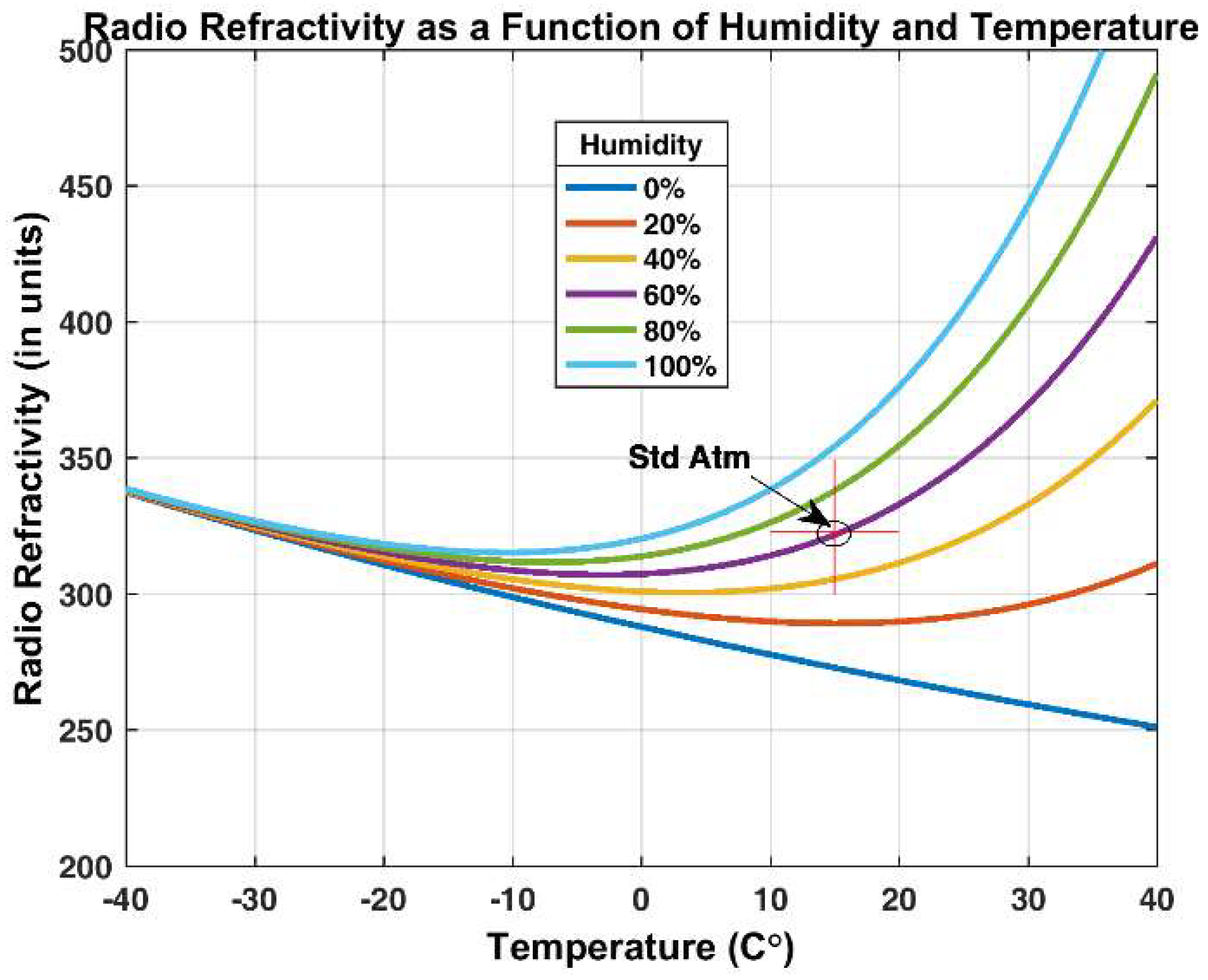
The variation in refractive index as a function of humidity and temperature is illustrated in Figure 4.
For temperatures below −10 °C, the humidity contributes little to the changes in N. Above −10 °C, the changes in humidity has a significant influence on N. In our study, a temperature variation between −20 °C to +25 °C is to be expected.
The electromagnetic distance R is
in which To is the travel time of the electromagnetic wave from the radar to the target and is the spatial and temporal index of refraction. A small change in range ΔR of a reflecting object will result in a proportional change in the phase Δφ of the following reflected signal:
in which is the wavenumber. Equation (3) is the definition of interferometry. The phase is ambiguous with integer multiples of 2π. To track motions by interferometry, we must be able to unwrap the phase correctly. This turns out to be a major challenge for long distances due to atmospheric variations. Assuming a stationary reflector, the observed variation in distance is due to variations in the index of refraction. This phase-variation is
To partly overcome this problem, a reference reflector may be used, enabling us to do differential measurements. This will eliminate the effect of atmospheric variation on the path between the radar to the reflectors, leaving only the path between the two reflectors. If we have two reflections represented by the complex numbers z1 and z2, the differential interferogram is
in which z* denotes the complex conjugate of z. The angle is computed by taking the inverse tangent of the following argument:
The differential interferometric phase i.e., the difference between z1 and z2, is the sum of the following multiple effects:
in which is the phase due to the displacement of the target, is the phase due to atmospheric delays, and is the phase noise due to the radar hardware.
When using interferometry the maximum unambiguous displacement is
The relation between the wavelength and the pulse repetition frequency (PRF) gives the following maximum unambiguous velocity:
In our case, we measure once a minute, giving a PRF of 1/60 Hz. The wavelength of the signal is λ9.65 GHz = 31.1 mm, giving a maximum unambiguous velocity of vmax = 129.4 µm s−1 or ~4.2 mrad·s−1. This gives a maximum unambiguous displacement per day of ~11.2 m.
Analytical expressions for the radar cross section (RCS) exist for some simple shapes including spheres, flat plates, and di- and trihedral. Apart from the sphere, the RCS of an object is heavily dependent on the frequency and the angle of the incident field. At Hegguraksla, we use triangular trihedrals reflectors. The analytical expression for the maximum RCS of a triangular trihedral is given as [4] (p. 25) as
in which a is the short side of the triangle and λ is the wavelength of the radar.
4. Data Processing
In this chapter, we present some basic measurements of the mountain and the pre-processing of the data. We start by analyzing the amplitude of the reflections from the corner reflectors. We then analyze the statistical distribution of the backscatter from the reflectors and the clutter from the mountain. By clutter, we mean the unwanted backscatter from all surfaces other than the reflectors. We then look at how the variation in radio refractivity affects the path length between the radar and the reflectors, and how snow build-up affects the measurements and the phase tracking. All analysis is based on data from radar measurements in Tafjord between 2nd March 2010 and 23rd March 2018.
4.1. Data Preprocessing
To avoid including corrupted data in our analysis, basic data cleaning is necessary before interferometric processing. The most probable cause of corrupted data is heavy atmospheric attenuation resulting in low amplitude levels. An amplitude cut-off value was set, and all measurements with values below this cut-off were rejected. During periods with heavy atmospheric attenuation, we have experienced attenuation in the order of 40–50 dB. Our experience from data collected in Tafjord is that we can track and unwrap the phase correctly with a signal attenuation of more than 20 dB. Based on this observation, the initial cut-off value was put at 30 dB below the one-hour moving average of the amplitude. The variation in amplitude level for all six reflectors during the measurement period is presented in the time-amplitude plot in Figure 5.
An illustration of the signal and noise problem is shown in Figure 6. The noise, N, is assumed to have a complex circular Gaussian distribution and is indicated by the red circle. Y is the actual backscatter, while A is the measured backscatter corrupted by the noise N. The measured angle ϕA differs from the actual angle by the noise angel. The noise is composed of variation in the clutter within the range-cell, variations in the refractivity, thermal noise, and instrument noise.
By using triangular corner reflectors, we increase the ratio between vector Y and N, hence reducing the influence the noise has on the phase of the backscatter. If the ratio Y:N decreases to a level at which the noise is larger than the signal, i.e., the noise space covering the origin, we will have severe problems unwrapping the phase, since A will randomly move from quadrant to quadrant.
After first eliminating measurements with values below the selected cut-off value, we use a statistical method to analyze the stability of the backscatter. Measurements with values below this statistical cut-off are rejected. We apply a method introduced by Ferratti et al. [9], originally intended as a way of identifying stable permanent scatterers in Synthetic Aperture Radar (SAR) data scenes. This is a measure for the phase stability called the dispersion index, defined as
in which mA is the mean value of the backscatter and σA is the standard deviation of the backscatter. This method is reported to give reliable results for high signal-to-noise (SNR) ratios, but without specifying what a high SNR is. The method is reported in [9,10,11] to give stable results with a threshold value typically around 0.25. Some of the shortcomings of the method like its tendency to overestimate the stability of the phase are pointed out in Appendix B in [12]. After applying this data exclusion method, we calculate the differential interferogram according to Equation (5).
4.2. Amplitude Variations
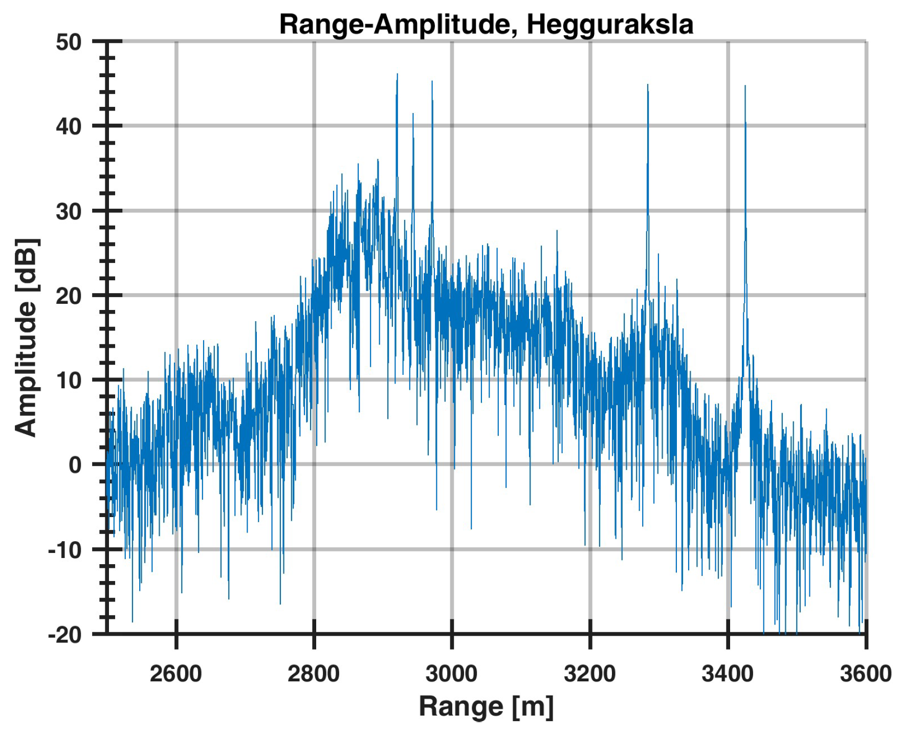
The range–amplitude plot presented in Figure 7 shows the backscatter from the mountain and the six corner reflectors. The results presented in Figure 7 are range-compensated by a range factor of R4 according to the radar equation [8].
The range in the plot is from 2500 m to 3600 m. The steep increase in backscatter level from 2700 m to 2800 m corresponds to the incline of the mountain. Equally, the backscatter level decreases from 2900 m to 3400 m as the slope of the mountain falls off. From 3500 m onward, we have only clear sky; this means that the backscatter is mainly from the side-lobes of the antenna. The triangular corner-reflectors dominate the backscatter from their respective range-cells, which implies that they can be treated as stable point targets. Table 2 shows mean amplitude values and standard deviation of the amplitude for the measurement period.
The backscatter is stable, except during periods with high atmospheric attenuation or occasional blocking of the antennas. When this occurs, the data acquired is rejected. For the lower two sites, the standard deviation of the backscatter is between 2 and 3 dB; for Site 3 the standard deviation is approximately 4 dB. The higher variation in backscattered energy at Site 3 is probably due to the longer range between the radar and the reflectors, which gives greater susceptibility to atmospheric attenuation.
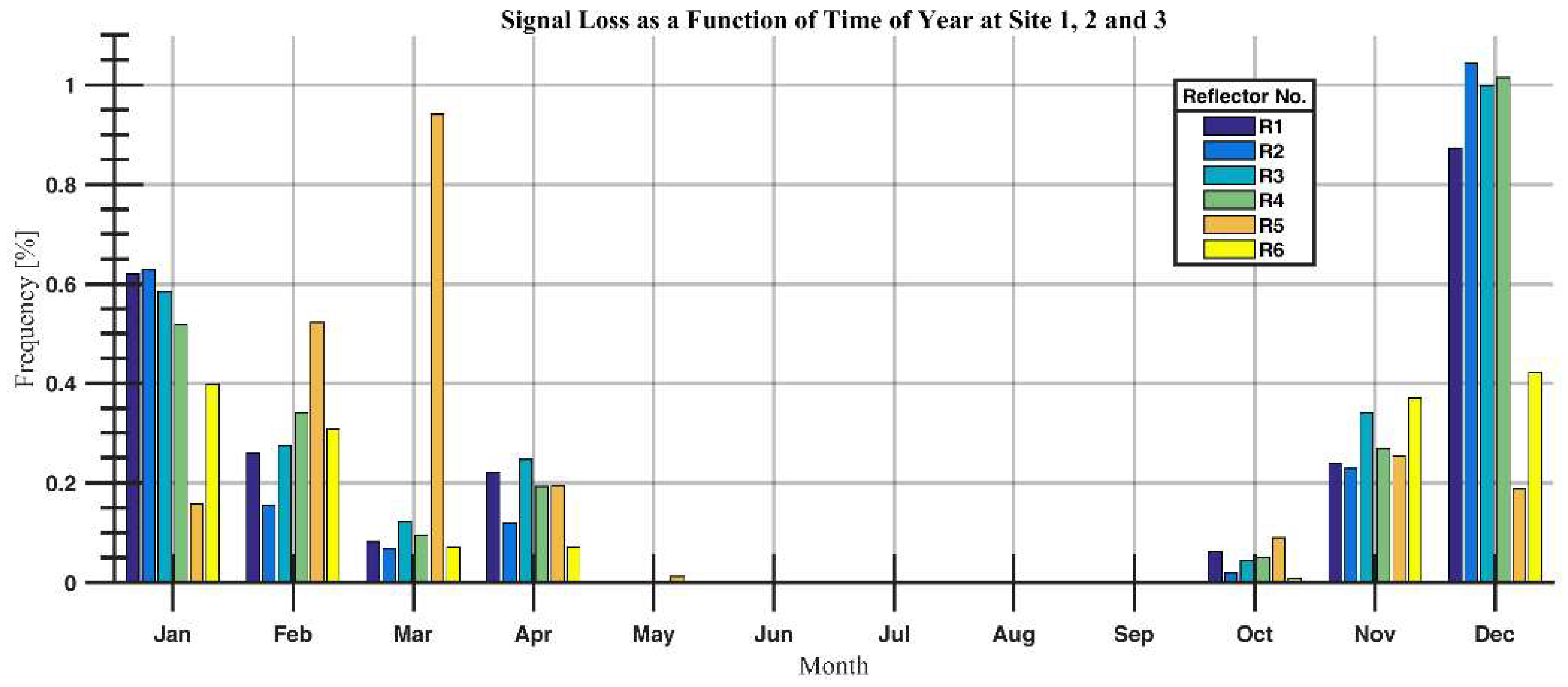
The majority of blocking due to attenuation occurs in the winter months and is believed to be caused by snow, especially wet snow or sleet (see Figure 8).
As can be seen from Figure 8, most of the fall-outs occur in the winter-months. There is a significant difference between the frequency of fall-outs in January and December between the two lower sites and Site 3 at the top of the mountain. The reason for this might be the difference in height, which means Site 3 might experience snow while the two lower sites have rain or sleet as the attenuation of rain or sleet is higher than dry snow. Another reason is the signal-to-clutter level, which is higher at Site 3 than at the two lower sites, refer to Figure 7.
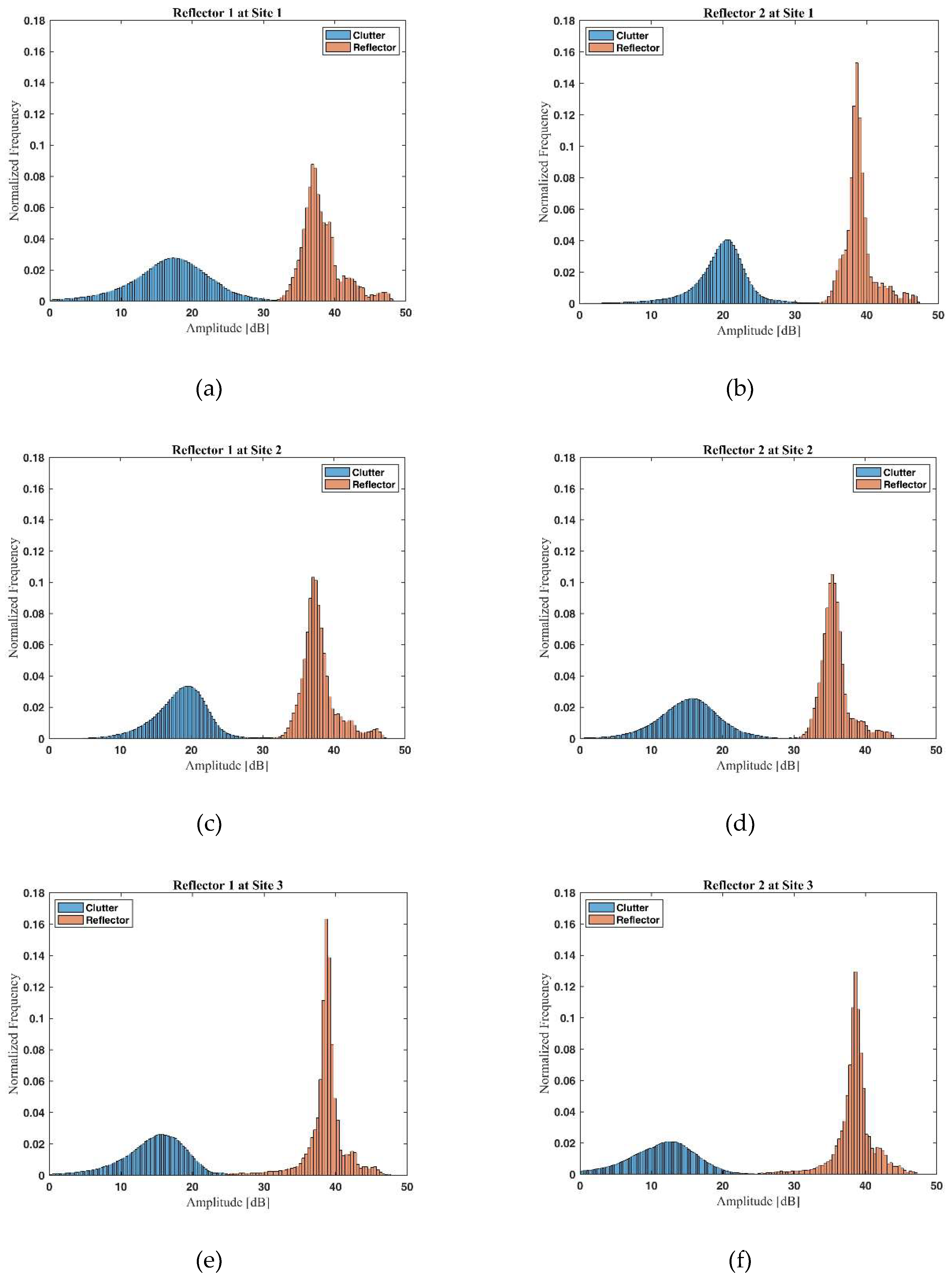
Comparison of the statistical distribution of the backscattered energy from the corner reflectors and the mountain gives further insight into the signal-to-clutter level to be expected. In Figure 9, histograms for the range-cell containing the reflector and nearby clutter from the 8 years of monitoring are shown.
The histograms are based on all data from 2nd March 2010 to 23nd March 2018. The reflectors are grouped horizontally per site (panel (a) and (b) are from Site 1, panel (c) and (d) are from Site 2, and panel (e) and (f) are from Site 3). The results show that the amplitude of the backscattered energy from the triangular corner reflectors is about 20 dB above the clutter level, making them easily detectable point targets. The result corresponds to the range–amplitude plot presented in Figure 7. These results support the assumption that the natural clutter from the mountain has a normal distribution while the artificial reflectors, being point targets, have a Rayleigh distribution [9].
4.3. Relation between Meteorological Data and Radio Refractivity
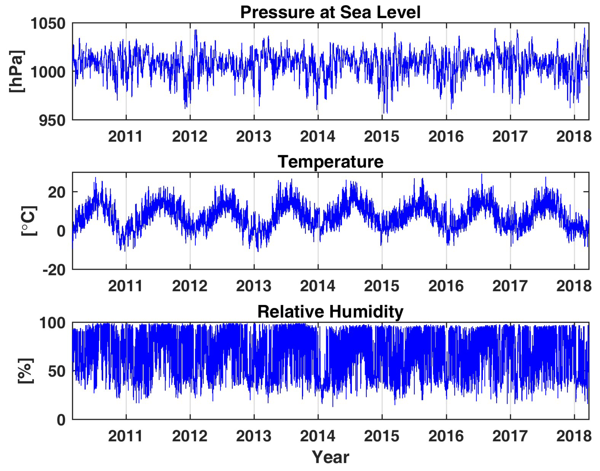
As presented in Section 3, meteorological data can be used to calculate the radio refractivity, and the results can be used to compensate the measurements for variations in the refractivity. The meteorological data used in this chapter is from The Norwegian Meteorological Institute’s measurement station in the village of Tafjord. The meteorological station is located at an altitude of 11 m AMSL and records meteorological data every sixth hour. This is not frequent enough to do post corrections of the measurements, but it can be used to show trends in the radio refractivity. Another weakness is the distance between the meteorological station and the radar, which is approximately 8.5 km. This adds uncertainty to the calculations. The measured pressure, humidity, and temperature is presented in Figure 10.
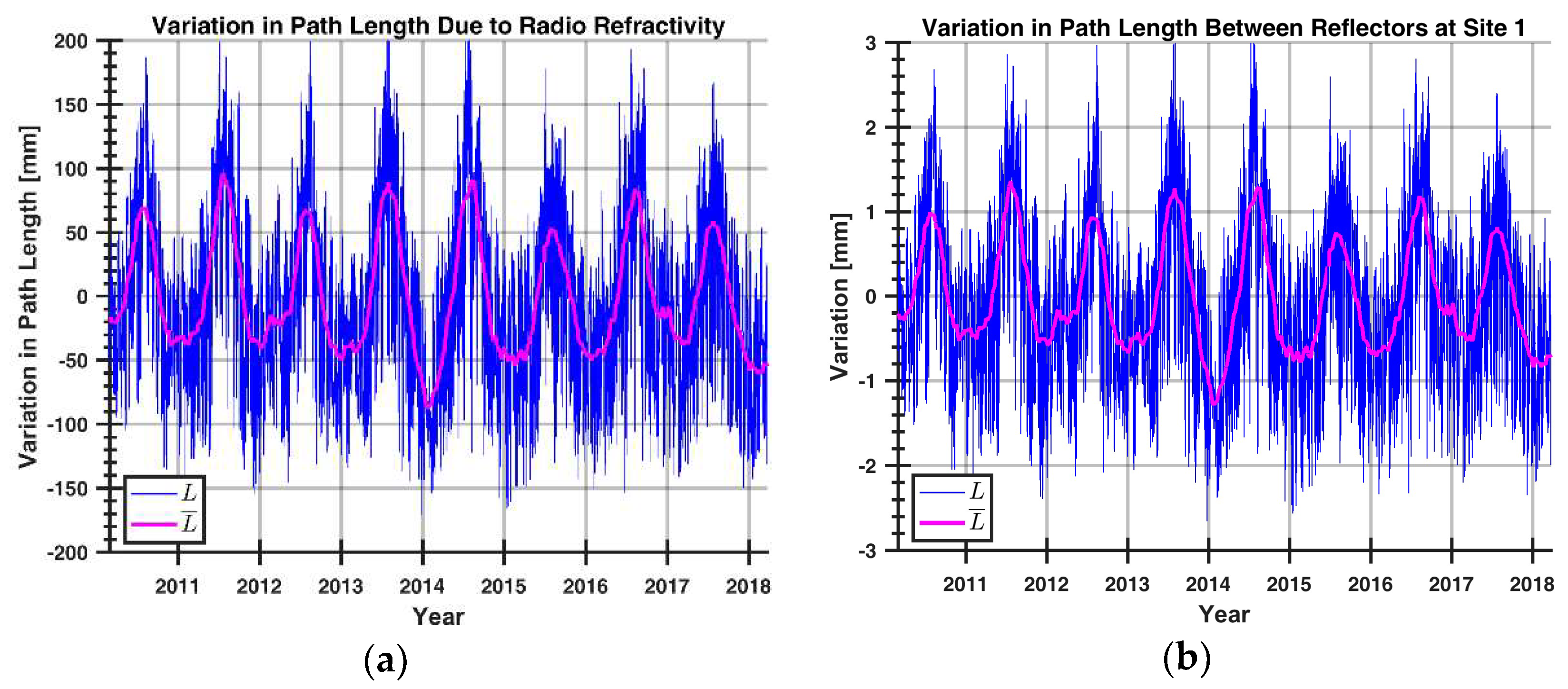
By estimating the variation in path length from the meteorological data presented in Figure 10, we can calculate the variation in path length for the path between the radar and the six reflectors. In Figure 11, we present the calculated variation in path length between the radar and reflector 1 at Site 1 and between the two reflectors at Site 1.
From Figure 11a, the estimated variation in path length between the radar and reflector 1 at Site 1 is almost 400 mm. From Figure 11b, the variation in path length between the two reflectors at Site 1 shows a total variation of about 6 mm. This illustrates the reduction in path length variation between differential and non-differential measurements. Estimated variation due to radio refractivity in radar-to-reflector path length for reflector 3 at Site 2 is 390 mm, while the variation between reflector 3 and 4 at Site 2 is 2.6 mm. This is a reduction in variation due to radio refractivity by a factor 150. For Site 3, the radar-to-reflector path length variation due to radio refractivity is 438 mm, while the variation between reflector 5 and 6 at Site 3 is 16.1 mm. This is a reduction in variation due to radio refractivity by a factor 27.
This eliminates a lot of uncertainty in the phase tracking and the phase unwrapping processes. Referring to Figure 6, the noise vector, N, is reduced accordingly. This clearly shows the benefit of the differential technique, which results in improved accuracy.
The distances between the reflectors and the estimated variation in path length due to refractivity both for differential and non-differential interferometry for the three sites are listed in Table 3.
Table 3 shows that by using differential interferometry, the variation due to radio refractivity can be significantly reduced. If we divide the variation in path length from radar-to-reflector by the radar-to-reflector distance, we get a factor of approximately 7.5:1. If we do the same with the reflector-to-reflector path length variation and reflector-to-reflector distance, we get a factor of approximately 9:1. The deviation in results might be explained by how the difference in height is accounted for in the radio refractivity model. Another issue is that the local atmospheric conditions in the mountain might deviate from the radar-to-reflector atmospheric conditions.
4.4. Impact of Snow on the Reflectors
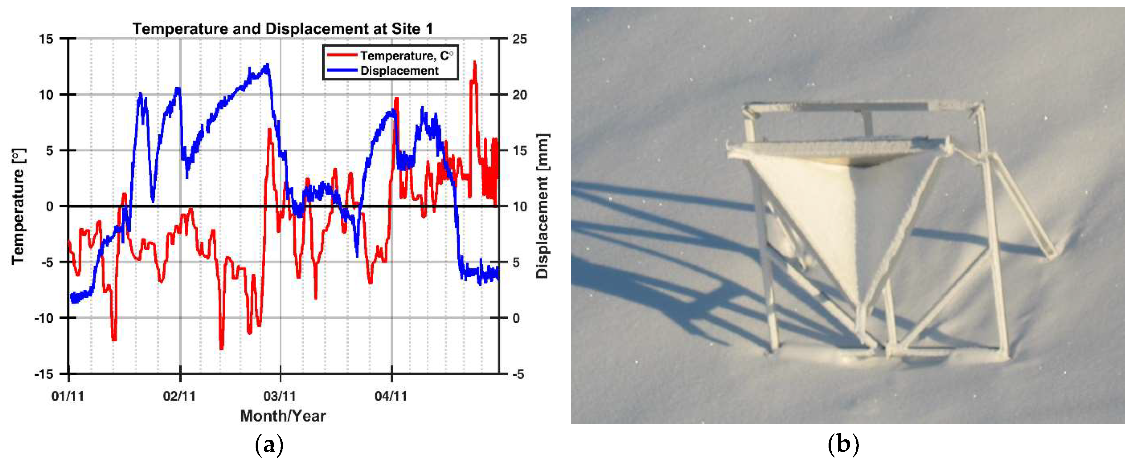
Over the years, we have experienced challenges when the reflectors are covered by snow. This will cause a phase tracking challenge, since we have no means of measuring the depth of the snow cover and compensating for the added path-delay. Figure 12a shows the effect of snow build-up inside the reference reflector at Site 1 during the winter of 2011. Figure 12b shows a picture taken of one of the reflectors during the winter of 2011.
The displacements presented in Figure 12a are believed to be caused by snow building up inside the reflector. This results in an increased distance due to the longer traveling path of the electromagnetic waves. By comparing the possible build-up of snow with the temperature profile, there is a good correlation between the calculated temperature and the snow build-up and the snow melting. Clearly identified in the end of February and beginning of March when the temperature rises, the snow inside the reflector melts, and the electromagnetic path length is once again reduced. The increase in distance at Site 1 during the winter of 2011 is tracked without loss of data, and the displacement before and after the snow build-up is within 1 mm. During the build-up and melting of snow in the winter of 2010, we lost the signal 5 times due to atmospheric attenuation, producing high uncertainty in phase unwrapping results.
The phase tracking in the winter of 2012 resulted in a displacement of more than 6 mm. This displacement is believed to be erroneous and a result of loss of signal due to heavy attenuation and snow build-up inside one or both reflectors at Site 1.
To check which of the reflectors at Site 1 were covered by snow, we compared the two reflectors at Site 1 with the reference reflector at Site 2. The comparison reveals that reflector 2 at Site 1 was covered by snow in the winters of 2011, 2012, and 2015. Reflector 1 at Site 1 showed no sign of being covered by snow. This result is supported by the placement of the reflectors at Site 1. The main reflector is right at the edge of the mountain, making it less likely to be exposed to snow drift, whereas the reference reflector is located at a more shielded position that is more likely to be exposed to snow drift.
5. Long Term Monitoring Results
In this chapter, we present the results from the long-term monitoring of the mountain with the ground-based radar in the period 2nd March 2010 to 23rd March 2018. The radar has been operational 96.4% of the time, in which major stops are due to faults on the mains power.
5.1. Diurnal Variations
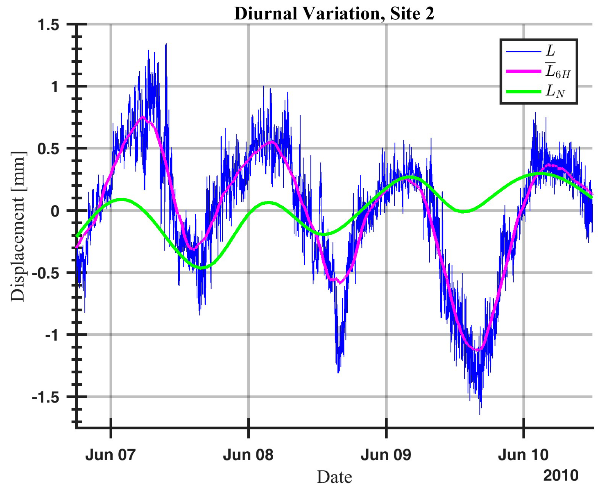
The data from the ground-based radar reveals diurnal variations in the measured path length using Equation (3). This variation is believed to be caused by diurnal variations in temperature and radio refractivity. An example from four days in June 2010 is presented in Figure 13.
The results presented in Figure 13 show a diurnal cyclic variation in path length between the two reflectors at Site 2. There is a good correlation between the measured path length variation and the calculated radio refractivity. However, the estimation of radio refractivity seems to underestimate the path length variation.
5.2. Annual Variations
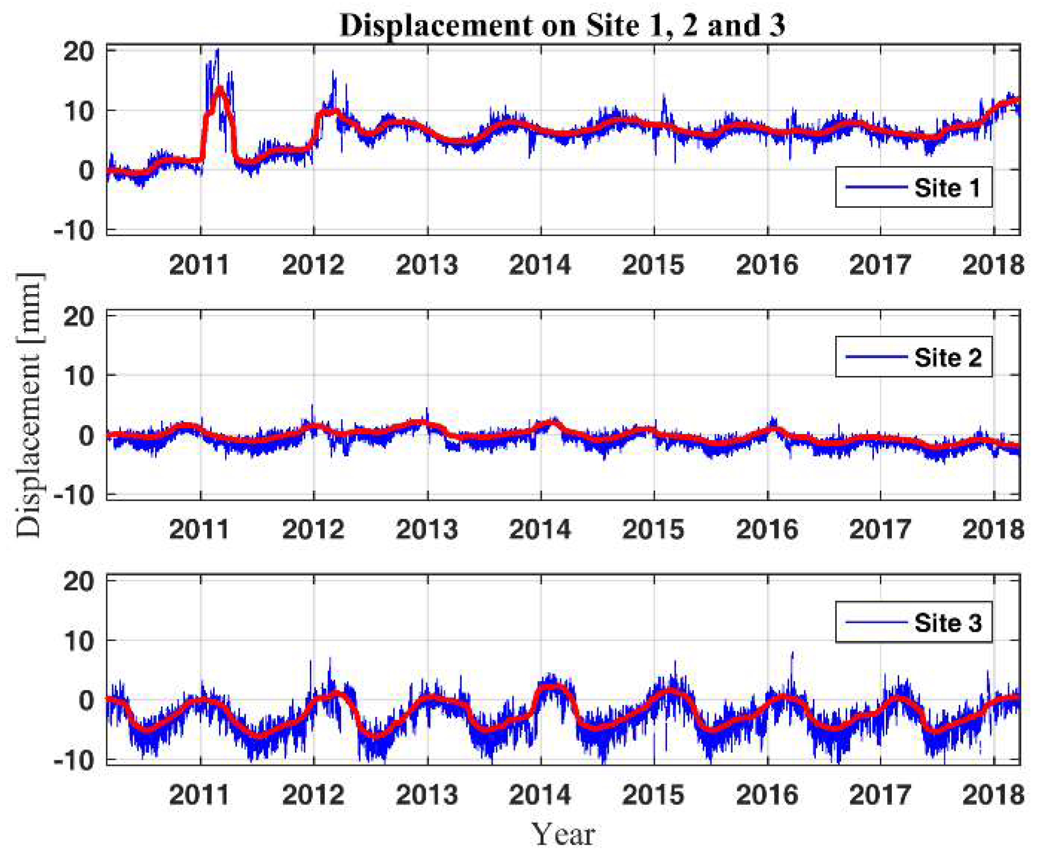
The path length to the reflector pairs at each site is calculated by differential interferometry, Equation (3), and the resulting time-displacement diagram for all three sites are presented in Figure 14. Negative values indicate a shorter path length between the radar and the reflectors.
When analyzing the results, we see an annual cyclic variation in the path length, especially at Site 3. This variation is in good correlation with the annual temperature variations; see meteorological data in Figure 10. There is significant variation in phase stability from site to site. Sites 3 and 1 have a significantly higher variation than Site 2. This is as expected, since the distance between the two reflectors at these sites is longer. The cumulative displacement at Site 1 is 4.7 mm, at Site 2 the displacement is approximately 1 mm, while Site 3 shows, as expected, no displacement. The large displacement at Site 1 is believed to be a result of snow build-up, which we were unable to track correctly during both build-up and melting (see Section 4.4).
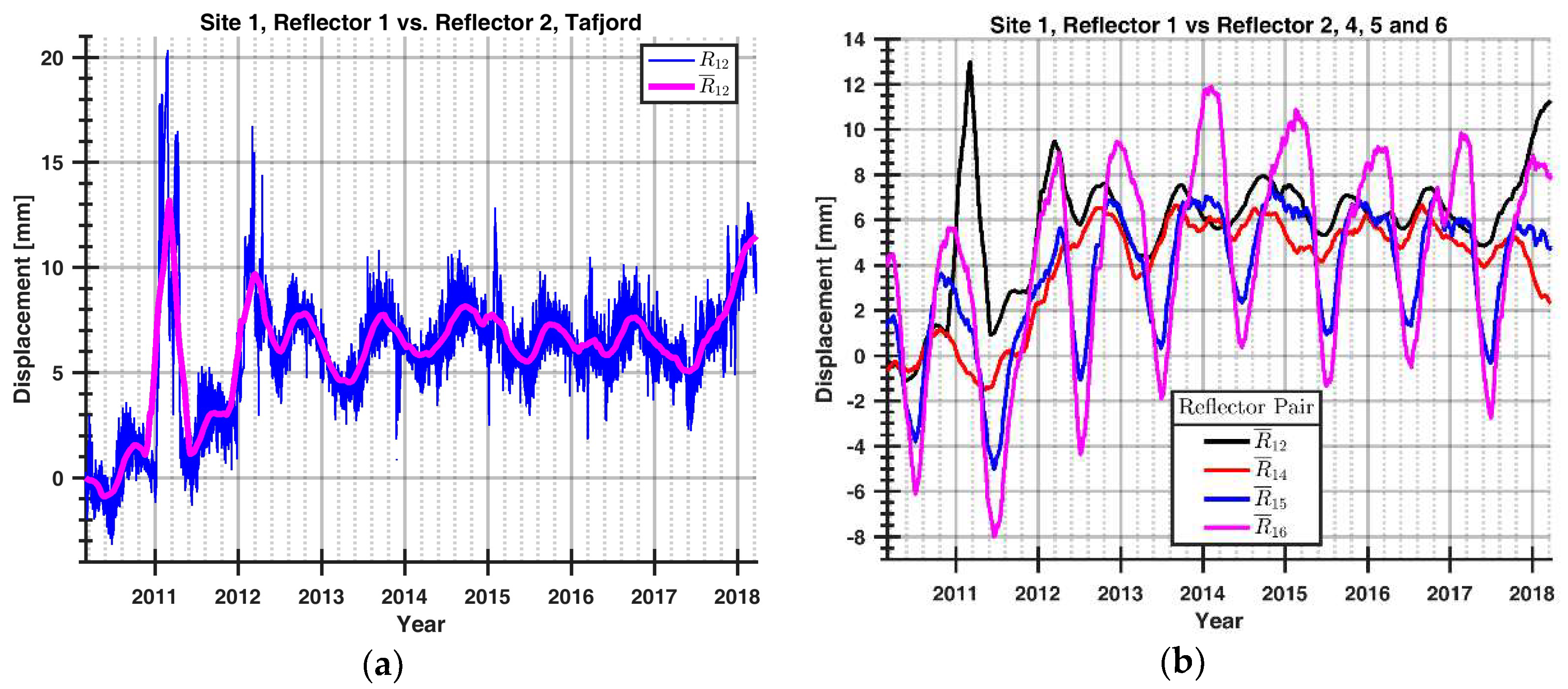
5.2.1. Estimated Motion at Site 1, Reflector 1
A detailed plot of the displacement of Site 1 as measured by the radar is presented in Figure 15a, both raw data and three-months moving mean. We also present the displacement of reflector 1 with respect to the four reference reflectors (reflectors 2, 4, 5, and 6, see Figure 2) in Figure 15b.
Figure 15a shows two interesting features: firstly, the three large displacements taking place during the first months of 2011, 2012, and 2018; and secondly, the displacement developing from the middle of 2011 to the middle of 2012 that is about 6 mm. According to geological analysis, the most probable reason is a rotation of the mountain block towards the fjord at the base and backwards at the top [13]. Other possible reasons are snow build-up inside the reference reflector or snow build-up behind the reference reflector permanently bending the beams securing the reflector to the mountain.
The comparison between the four reference reflectors presented in Figure 15b shows the same trend but with some differences. The amplitude of the annual cyclic variations gets higher as the distance between the reflectors compared increases. This result is supported by the results presented in Section 4.3 and is due to the radio refractivity caused by variation in path length. Only the results from Site 1 show a pronounced displacement in the winter of 2011 and 2018, further supporting the belief that reflector 2 at Site 1 was covered by snow. The displacement occurring in the winter of 2011–2012 is present in all the data, indicating a backwards motion of the block. This assumption is supported by the geological analysis of the mountain block as it is moving outwards at the base, which implies an inward rotation of the top of the block [13]. An inwards rotation of the top would result in an increased radar-to-reflector path, which is what we observe in the winter of 2011–2012.
The measured displacement of reflector 1 at Site 1 compared to the four reference reflectors is given in Table 4.
The reason why the standard deviation of reflector 2 at Site 1 is higher than the standard deviation of reflector 4 at Site 2 is probably due to the partial loss of reflector 2 in the winters of 2011, 2012, and 2015.
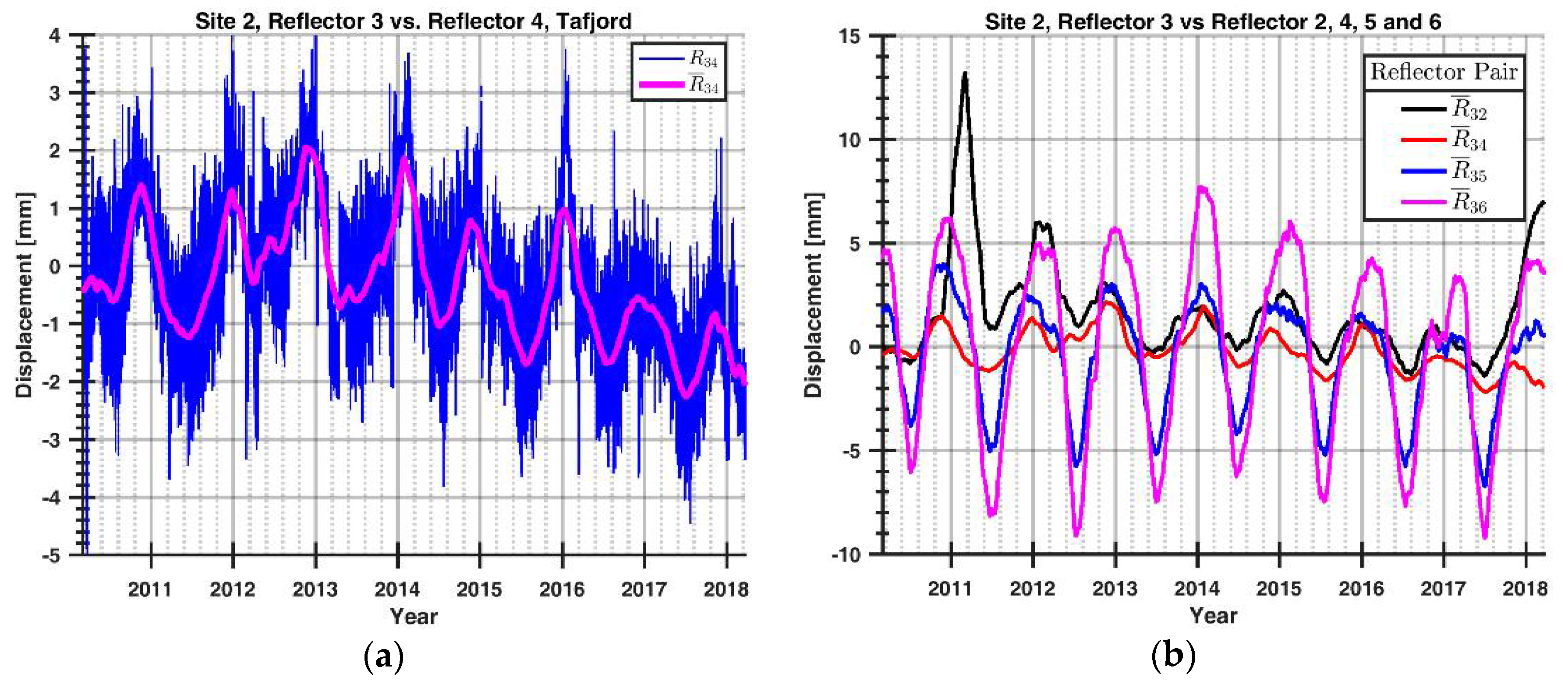
5.2.2. Estimated Motion of Site 2, Reflector 3
A detailed plot of the measured displacement of Site 2 is presented in Figure 16a, both raw data and three-months moving mean. To verify the displacement at Site 2, reflector 3 is compared to all the four reference reflectors (reflectors 2, 4, 5, and 6, see Figure 2) in Figure 16b.
The total displacement from 2010 to 2018 is in the order of −1.2 mm. The annual cyclic variations are clearly visible in Figure 16. The measurements seem to be stable for the first two years and then show a motion away from the radar during the last 6 months of 2012. From 2013 onwards, there seems to be a steady motion towards the radar. The displacement from 2013 to 2018 is in the order of −2.0 mm.
Reflector 3 shows the same displacement pattern when compared to the four reference reflectors, with the major differences being the variation in the amplitude of the annual cyclic variations. The Site 2 comparison is summed up in Table 5.
There is a significant motion of the mountain block of approximately 2 mm from 2013 to 2018. The major direction of motion of the block is believed to be vertical with an outwards motion at the base [13].
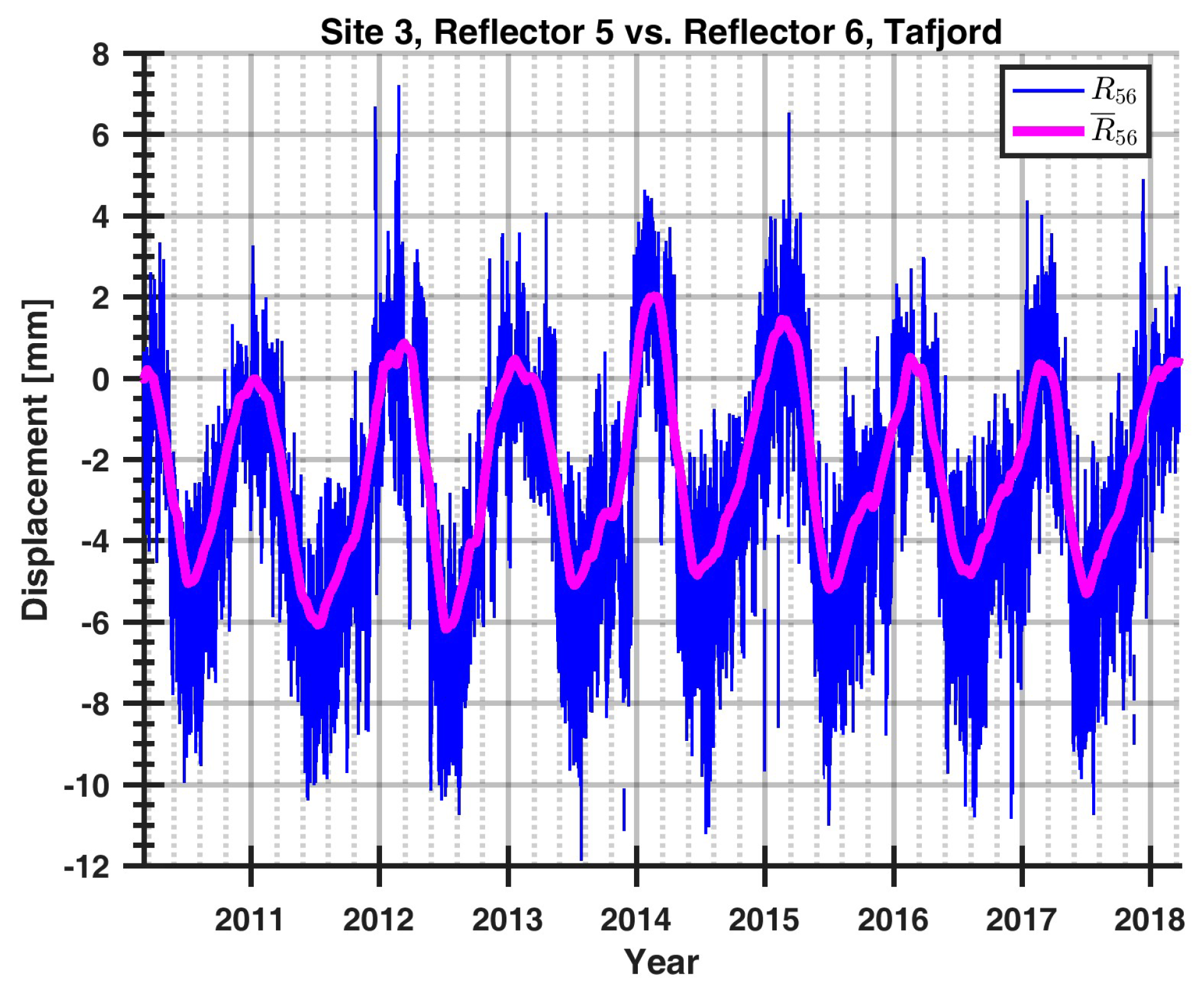
5.2.3. Estimated Motion at Site 3, Reflectors 5 and 6
We have not detected any motion between reflectors 5 and 6 at Site 3, except annual cyclic motions that are believed to be caused by temperature variations, see Figure 17.
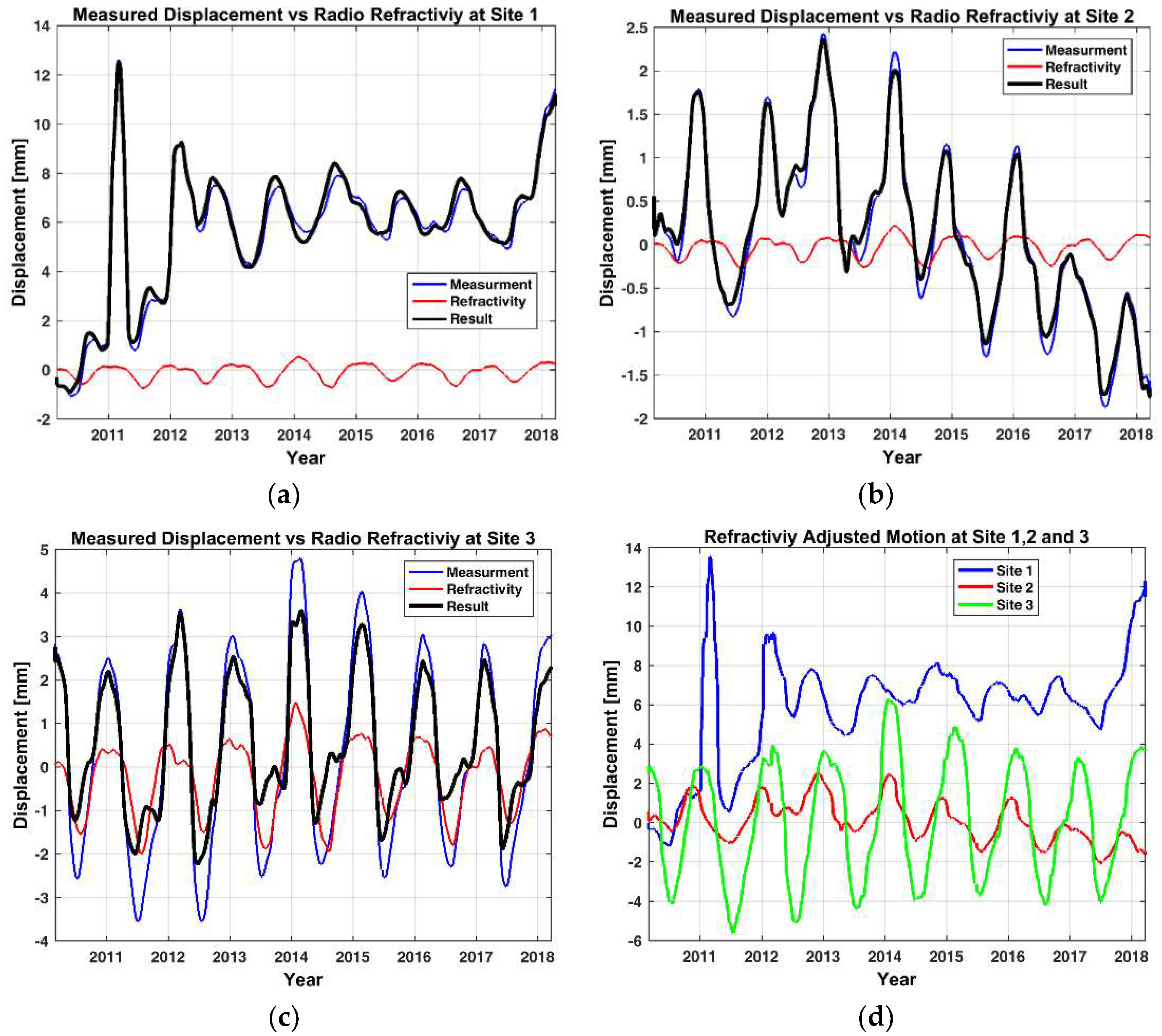
For reference, a comparison of differential interferometric measurements with and without radio refractivity corrections applied to the path length between the reflectors is presented in Figure 18.
As shown by Figure 18, the result for Site 3 shows a good correlation between the estimated refractivity and the calculated differential interferometric displacement. The annual variation is reduced by nearly 35%.
6. Comparison of Displacement with Other Measurement Methods
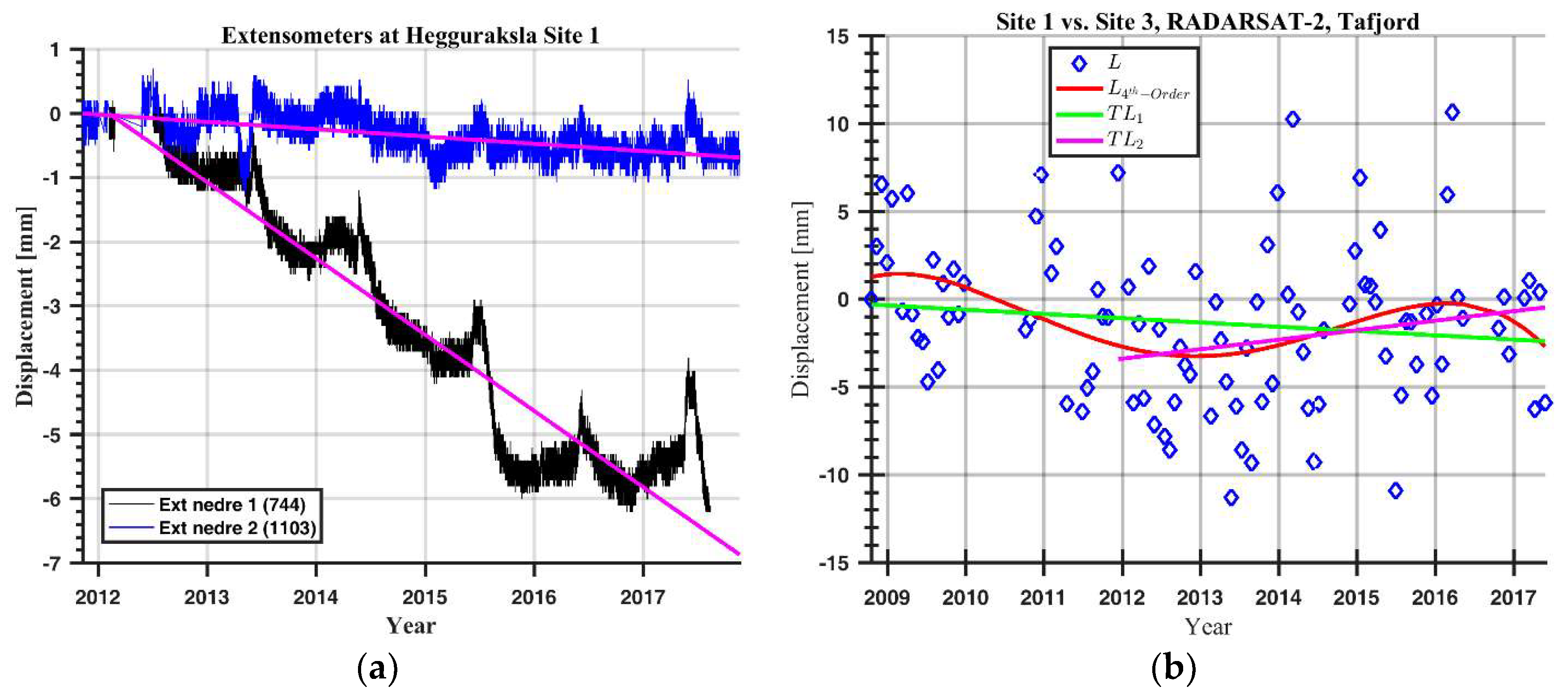
The two unstable blocks at Hegguraksla are in addition to the ground-based radar monitored by spaceborne radar and geotechnical instruments like extensometers and crackmeters. At Site 1, two extensometers have been operational since February 2012. The extensometer data is collected every 30 min; this data was kindly made available from the Åknes/Tafjord Beredskap IKS [13] (see Figure 19a). We also have data from the Earth Observation Satellite RADARSAT-2 owned by the Canadian Space Agency. This data was kindly made available for us from Norut [14] (see Figure 19b). This is a spaceborne radar, and all measurements are line-of-sight (LOS) and not converted to vertical displacemet. The two triangular corner reflectors used for the SAR measurements are located close to Site 1 and Site 3. At Site 1, we share foundation with the SAR-reflector.
From Figure 19, we see that the data from the two extensometers differ significantly; the one with reference number 744 has a recorded displacement of −0.7 mm, and the one with reference number 1103 has a recorded displacement of −6.0 mm. The motion of extensometer 2 is believed to be partly due to failure of the mounting rods at one end. Table 4 shows our measurements, which vary from 4.7 mm to 6.1 mm. The vertical displacement trend of the satellite reflector at Site 1 referenced to the satellite reflector at Site 3 from 2008 to 2017 is −2.1 mm, and from 2012 to 2017 is 2.1 mm. There are 98 samples available for this 8-years period.
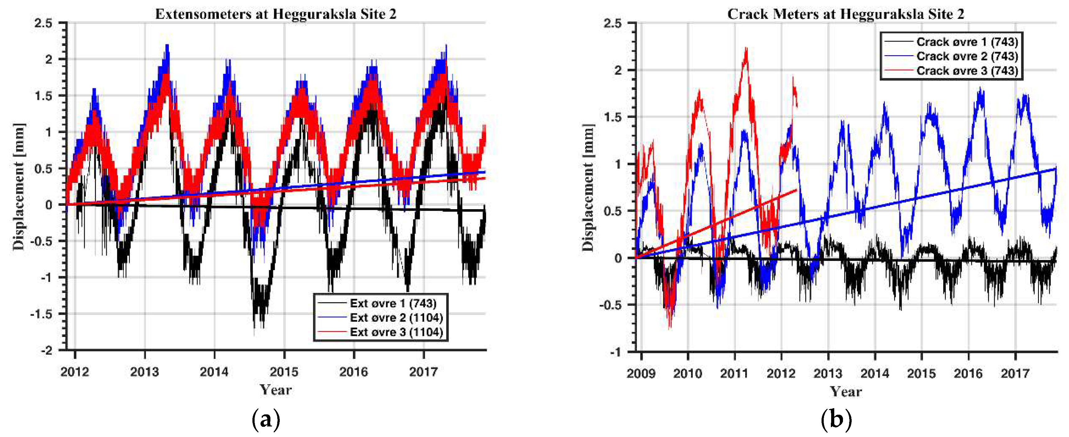
At Site 2, there are three extensometers and three crack meters. These data were also made available for comparison with the radar data (see Figure 20).
All six instruments show different displacements due to the way they are mounted. It is interesting to note the distinct annual cyclic motion, which is in good correlation with the cyclic variation measured by the radar.
7. Discussion
We have conducted eight years of continuous measurements with ground-based interferometric real-aperture radar of two unstable mountain blocks at Tafjord on the western coast of Norway. With this relatively long measurement period, we are able to assess and discuss several aspects of the project: the measurement uncertainties due to periodic changes on various timescales in atmospheric conditions typical for the local marine environment, applied measurement corrections, practical challenges of the established radar set-up shown in Figure 2, and measurement uncertainties relative to typical seasonal geological movement determined by other types of sensors. All sensors have their strengths and weaknesses, noise sources, and measurement errors, and measurement noise is displayed for extensometers in Figure 19 and Figure 20a, crack meters Figure 20b, SAR Figure 19b, and ground-based radar Figure 13. It is beyond the scope of this article to discuss the error sources of geotechnical instruments, and in the following we will focus on error sources in interferometric ground-based radar. In general, the results presented show that a ground-based radar is a valuable supplement to, or substitute for, in situ geotechnical instruments.
The radar measurements show amplitude variation in backscatter from the reflectors due to variations in atmospheric attenuation and radio refractivity on various timescales. The fast variations between radar pulses are believed to be caused by rapid but small changes in the radio refractivity, see Figure 13. The diurnal and annual changes are believed to be mainly caused by temperature changes. The variations in atmospheric attenuation are mainly caused by the changing weather, which affects the accuracy of the measurements of the reflectors for three reasons. First, attenuation can lead to a total loss of signal resulting in missing data. Second, varying attenuation between the reflector-pairs compared differentially is a potential error source. An example is build-up of snow in one of the reflectors, see Figure 12. This will lead to drift in measured range, and unless it is possible to follow the build-up and the melting of the snow, we are unable to unwrap the phase correctly. Third, if the temporal variation in the atmosphere is faster than the measurement rate, it may introduce unwrapping ambiguities leading to uncertainties in the results (see Equation (7)). The variation in radio refractivity results in variation in the radar-to-reflector path length.
Based on the results from over eight years of monitoring of Hegguraksla Mountain, we have observed that the amplitude of the annual cyclic motion exceeds the displacement of the mountain blocks (see Figure 15, Figure 16 and Figure 17). This is also shown in the results from the extensometers and crackmeters (see Figure 20). Thus, the measurement period must extend annual cyclic geologic movements believed to be caused by annual changes in temperature. This implies that the measurement period must exceed multiple annual cycles before any conclusions can be made with respect to actual mountain block displacements.
Statistical analysis of the radar backscattered energy shows that the triangular corner reflectors with a signal-to-clutter level of approximately 20 dB provide stable point targets for real-time monitoring (see Figure 9). The reflectors ensure that we monitor the unstable mountain blocks on which they are mounted and not the surrounding mountain area. The use of mounted corner reflectors are in our opinion the best way to ensure monitoring of specific points of interest with a minimum of noise.
Corrections for the variation in radio refractivity between the reflectors have been applied on the measured relative path length of the reflectors, and this has been successful to some extent. For Site 1 and Site 2, the correlation between the calculated path length due to radio refractivity and the measured path length is weak, and the effect of applying the refractive correction is low. Local variation in the boundary layer conditions with height is not registered with the single meteorological station at sea level. Another weakness of the meteorological data used for the applied radio refractive correction is the horizontal distance of 8.5 km between the meteorological station and the radar site, which opens for variations in the atmosphere across the fjord. The lack of correlation between the calculated radio refractivity and the measured motion at Sites 1 and 2 is believed to be due to a more complex atmospheric environment than at Site 3. Site 3 is located at the top of the mountain, and there are no obstructions around the two reflectors, which probably gives a more homogeneous atmosphere. Both Sites 1 and 2 are located at the edge of the mountain and may be influenced by rising or falling air. The rapidly rising or falling air may be very turbulent, which is not taken into account by the radio refractive model. The model assumes linear changes in temperature, pressure, and humidity as a function of height. One possible way to improve the corrections is to have a weather station at each site and one at the radar, reducing the uncertainty in the refractive estimates.
A practical implication of the established radar set-up is the seasonal variations in snow cover during winter, shown in Figure 2. As shown in the measurement results (see Figure 12 and Figure 15), the reference reflector at Site 1 has suffered from snow cover on three occasions during the eight years of monitoring. As we have four reference reflectors in our set-up, we compared the main reflector at Site 1 to the other three reference reflectors. The result indicates that the reference reflector was covered by snow, but by using the other reference reflectors the motion of the main reflector could be followed. This solves the problem, but increases the uncertainty in the results, as the distance to the other reference reflectors is longer. This problem can be solved by protecting the reflectors with snow protection-covers. Snow on the ground is a general problem in real-time monitoring, as the snow will affect the backscatter from the ground. It will result in both attenuation and a variation in path length due to the higher dielectric constant in the snow. Therefore, an uneven snowfall or thaw will appear as measured divergent motion. The use of radar reflectors will improve the measurement results, particularly under these types of measurement conditions.
The measurement uncertainties are assessed relative to typical seasonal geological movement measured by other sensors (see Figure 19 and Figure 20). At Site 2, the results from the seven sensors (three extensometers, three crack meters, and the radar) all show the same seasonal cyclic motion. There is a spread in the results from these sensors, which is mainly believed to be determined by which part of the motion they measure, i.e., how they are mounted with regard to the motion of the mountain block. The annual variation in motion measured by the radar is ±1 mm. This agrees with the annual variations measured by the extensometers and crack meters, which are between ±0.3 mm and ±1.5 mm. The annual cyclic motion measured by the radar and the geotechnical instruments is coherent with the cyclic pattern of meteorological data, which indicates that the observed cyclic motion is due to temperature variations. Disagreement between radar results and the results from the geotechnical instruments is probably a result of the relative motion measured by the geotechnical instrument. At Site 1, the data from the extensometers show no correlation with the seasonal cyclic motion measured by the radar. It is not clear why the extensometers at Site 1 do not show the cyclic motions while both the extensometers at Site 2 and the radar measurements from Site 1 do, as this should be independent from the mounting direction of the extensometers. The spread in the results from the two extensometers at Site 1 makes it hard to compare it directly with the radar measurements. We have compared the results from the main reflectors at Site 1 and Site 2 with all the reference reflectors, and the results show good correlation, supporting the accuracy of the radar results.
The results show that real-time monitoring is challenging in areas occasionally exposed to snow, as the majority of the radar signal fallouts occur is in the winter season (see Figure 8). During periods with heavy snow or sleet, the atmospheric attenuation can interrupt the monitoring. Whenever this happens, we get discontinuities in the data set, which last until an adequate signal level is restored. This is, in our opinion, the largest weakness of the current measurement set-up and the presented results. Based on the Hegguraksla monitoring results, it would be beneficial to apply a snow protection-cover or relocate the reference reflector at Site 1 to a location less exposed to snowdrift.
8. Conclusions
In this paper, we have presented eight years of mountain monitoring with a real-time differential interferometric ground-based radar. We have shown that the radar can produce reliable, long-time, weather-independent output and that results from the radar measurements are as accurate as in situ measurements with geotechnical instruments, making it possible to remotely monitor inaccessible areas with high accuracy. The eight years of monitoring Site 1 shows a backwards motion between 4.7 mm and 6.1 mm. Based on the geological analysis of the mountain block, this motion is believed to be a geologic motion in which the block moves away from the mountain at the base and against the mountain at the top. Results for Site 2 reveal a sliding motion away from the mountain between 1.2 mm and 6.3 mm. This is also consistent with the geological analysis of the block at Site 2. The data collected show diurnal and annual variation mainly caused by variations in temperature and radio refractivity. The results show that for high accuracy monitoring, differential interferometry is preferable to non-differential interferometry, as it is less susceptible to variations in radio refractivity. We have also shown that variation due to radio refractivity can be reduced by using meteorological data to predict variations in radio refractivity and apply it to the measurements. For stable and predictable long-term surveillance, we recommend using reflectors mounted in the mountain that give a stable point-reflection. For real-time monitoring in changing atmospheric conditions, a high temporal sampling-rate is a prerequisite for interferometric measurements to avoid unambiguity in the unwrapping of the phase.
The results show both diurnal and annual cyclic variations, which means that we need a monitoring period of at least one year before making any conclusions about displacements, unless the displacement is larger than the diurnal and annual variations.
Snow cover of the reflectors causes a phase-tracking challenge if combined with heavy attenuation or loss of the radar signal. Based on the monitoring results, it would be beneficial to relocate the reference reflector at Site 1 to a location less exposed to snowdrift.
Future enhancements to the system should include a higher rate of measurement in order to avoid phase unwrapping ambiguities. There should be at least one local meteorological station close to the radar, preferably two stations, with the second at the base of the mountain. Additionally, there should be meteorological stations at each site due to the difference in height between the three sites, and the meteorological station should have a sampling rate high enough to compensate for rapid weather changes.
Author Contributions
Conceptualization: R.G. and R.N.; data curation: R.G.; formal analysis: R.G.; investigation: R.G.; methodology: R.G., R.N., and C.R.D.; software: R.G.; supervision: R.N. and C.R.D.; visualization: R.G.; writing—original draft: R.G.; writing—review & editing: R.G., R.N., and C.R.D.
Acknowledgments
The work was supported by the Research Council of Norway.
Conflicts of Interest
The authors declare no conflict of interest.
References
- Banholzer, S.; Kossin, J.; Donner, S. The Impact of Climate Change on Natural Disasters, Reducing Disaster: Early Warning Systems for Climate Change; Singh, A., Zommers, Z., Eds.; Springer: Dordrecht, The Netherlands, 2014; pp. 21–49. [Google Scholar] [CrossRef]
- Hole, J.; Blikra, L.H.; Anda, E. Scenario and prognoses for mountain avalanches and flodwaves from Åknes and Hegguraksla, Åknes/Tafjord Beredskap. Stranda, 2010. (in Norwegian) [Google Scholar]
- Oppikofer, T. Detection, Analysis and Monitoring of Slope Movements by High-Resolution Digital Elevation Models. Ph.D. Thesis, Institute of Geomatics and Analysis of Risk, University of Lausanne, Lausanne, Switzerland, 2009. [Google Scholar]
- Norland, R.; Gundersen, R. Use of radar for landslide hazard monitoring, Landslides and Avalanches, ICFL 2005 Norway. In Proceedings of the 11th International Conference and Field Trip on Landslides, Norway, 1–10 September 2005; ISBN 9780415386814. [Google Scholar]
- Norland, R. Differential interferometric radar for mountain rock slide hazard monitoring. In Proceedings of the 2006 IEEE International Symposium on Geoscience and Remote Sensing, Denver, CO, USA, 31 July–4 August 2006; pp. 3293–3296. [Google Scholar] [CrossRef]
- Rolstad, C.; Norland, R. Ground-based interferometric radar for velocity and calving-rate measurements of the tidewater glacier at Kronebreen, Svalbard. Ann. Glaciol. 2009, 50, 47–54. [Google Scholar] [CrossRef]
- Norland, R. Improving interferometric radar measurement accuracy using local meteorological data. In Proceedings of the Geoscience and Remote Sensing Symposium (IGARSS), Barcelona, Spain, 23–28 July 2007; pp. 3293–3296. [Google Scholar] [CrossRef]
- Levanon, N. Radar Principles; John Wiley & Sons: Tel-Aviv, Isreal, 1988; ISBN 0471858811. [Google Scholar]
- Ferretti, A.; Prati, C.; Rocca, F. Permanent scatterers in SAR interferometry. IEEE Trans. Geosci. Remote Sens. 2001, 39, 8–20. [Google Scholar] [CrossRef] [Green Version]
- Kampes, B.M. Radar Interferometry, Persistent Scatterer Technique; Springer: Dordrecht, The Netherlands, 2006; ISBN 140204576-X. [Google Scholar]
- Noferini, L.; Pieraccinin, P.; Mecatti, D.; Luzi, C.; Atzeni, C.; Tamburini, A.; Broccolato, M. Permanent scatterers analysis for atmospheric correction in ground-based SAR interferometry. IEEE Trans. Geosci. Remote Sens. 2005, 43, 1459–1470. [Google Scholar] [CrossRef]
- Hooper, A.; Segall, P.; Zebker, H. Persistent scatterer interferometric synthetic aperture radar for crustal deformation analysis, with application to Volcán Alcedo, Galpágos. J. Geophys. Res. 2007, 112, B07407. [Google Scholar] [CrossRef]
- Anda, E.; The Norwegian Water Resources and Energy Directorate, Oslo, Norway. Personal communication, 2018.
- Lauknes, T.R.; Northern Research Institute, Tromsø, Norway. Personal communication, 2017.
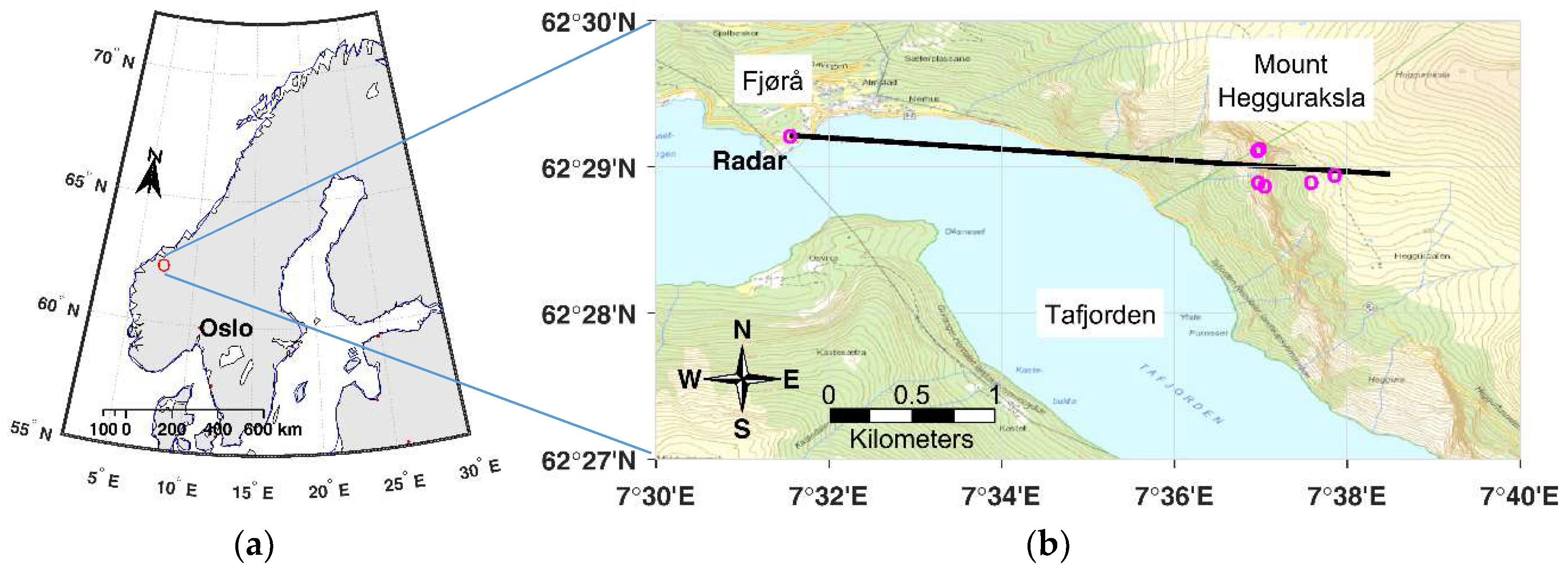
Figure 1.
Two maps showing the location of the radar. (a) Overview map showing where in Norway the radar is located. (b) Shows a detailed map of the studied area. The circle to the left marks the location of the radar, and the 6 circles to the right marks the monitored mountain area. The black line marks the pointing direction of the radar.

Figure 2.
Illustration of the measurement setup at Hegguraksla. There are three sites in the mountain with two reflectors at each. The numbering of the six reflectors is indicated below each reflector. The radar is located roughly 3 km from the mountain. The triangular corner reflectors are located from 740 to 1000 m AMSL.

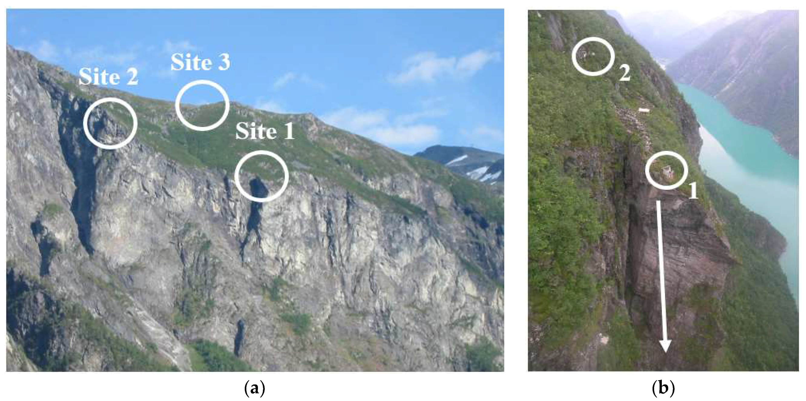
Figure 3.
(a) Hegguraksla Mountain viewed from Fjørå where the radar is located. The three areas (Sites 1–3) are marked with white circles. (b) is a close-up picture of Site 1, showing the vertical fault and the location of reflector 1 and 2. Reflector 1 is the main reflector, and 2 is the reference reflector. The white arrow indicates the anticipated motional direction of the block.

Figure 4.
Variation in refractive index as a function of air temperature and relative humidity. The pressure is kept constant at 1013.25 mbar. The International Standard Atmosphere according to ISO 2314 is marked with a red cross-hair (The ISO 1314 Standard Atmosphere is defined as Temperature = 15°C, Humidity = 60% and Pressure = 1013.25 mbar at Sea Level).

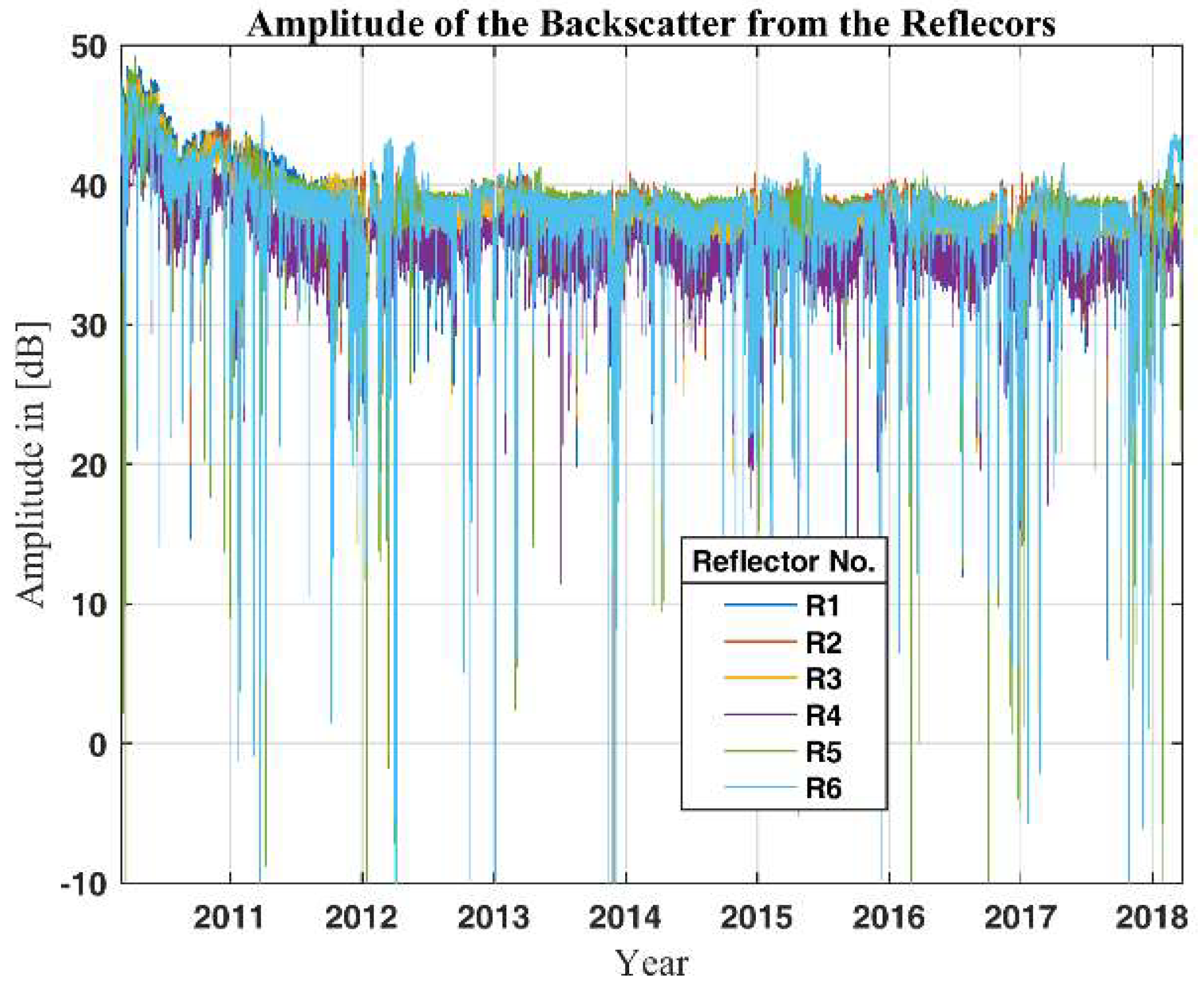
Figure 5.
Time-Amplitude plot showing the amplitude of the reflected energy from the six reflectors as a function of time. Most of the attenuation is in the winter-months, which for this part of Norway and this elevation is from November to March.
Figure 5.
Time-Amplitude plot showing the amplitude of the reflected energy from the six reflectors as a function of time. Most of the attenuation is in the winter-months, which for this part of Norway and this elevation is from November to March.

Figure 6.
Phasor plot illustrating the amplitude and phase contribution. A is the amplitude of the measured backscatter from one range-cell. N is the sum of the noise and Y the actual backscatter from the reflector. ϕA is the measured angle and ϕN the angle of the noise contribution. The red circle illustrates the circular sample space of the noise.

Figure 7.
A section of the range–amplitude plot showing the distinct reflections from the six triangular corner reflectors. Note that the first peak contains both reflectors 1 and 3, as they are separated by just three range-cells. The range plot is range-compensated for by a range factor of R4 according to the radar equation [8]. The corner reflectors are in a range from 2900 to 3400 m. The radar cross section of the reflectors is 36.2 dBsm at 9.65 GHz.

Figure 8.
The percentage of time per month that the signal has fallen below the cut-off value for the measurement period. Most of the fall-outs occur in the winter.
Figure 8.
The percentage of time per month that the signal has fallen below the cut-off value for the measurement period. Most of the fall-outs occur in the winter.

Figure 9.
The variation of the amplitude reflects the signal-to-clutter level of each corner reflector. Panel (a) and (b) are from Site 1, panel (c) and (d) are from Site 2, and panel (e) and (f) are from Site 3. High signal-to-clutter level produces low variation. The amplitude of the backscattered energy from the reflectors shows a Rayleigh distribution as stated in [9], while the clutter from the mountain is normally distributed.

Figure 10.
Meteorological data showing pressure, temperature, and relative humidity from March 2010 to March 2018. The meteorological data are from The Norwegian Meteorological Institute’s measurement station in Tafjord, located approximately 8.5 km from the radar.
Figure 10.
Meteorological data showing pressure, temperature, and relative humidity from March 2010 to March 2018. The meteorological data are from The Norwegian Meteorological Institute’s measurement station in Tafjord, located approximately 8.5 km from the radar.

Figure 11.
Panel (a) shows the estimated variation in path length between the radar and reflector 1 at Site 1 due to variations in the radio refractivity. Panel (b) shows the path length variations between the two reflectors at Site 1. The blue line is the raw-data, while the magenta line is 3-month moving mean. The variation in path length due to radio refractivity is reduced by a factor of approximately 66 when using the differential technic.

Figure 12.
(a) Variation in path length and estimated temperature profile as a function of time at Site 1 during the first four months of 2011. This variation is believed to be caused by build-up of snow inside the reflector. Please note that even though the variation at the end of January seems to be instantaneous, the maximum measured velocity is in the order of 2 mrad·s−1, which is about half the maximum unambiguous velocity of the radar (vmax = 4.2mrad·s−1). The temperature profile is based on the meteorological data presented in Figure 10. Even though the meteorological data is from a station 8.5 km away, it gives an indication of the temperature at Site 1. There is a good correlation between the temperature profile and the measured displacement of the reflector. (b) Picture of build-up of snow inside one of the reflectors during the winter of 2011. The photo is from Åknes-Tafjord IKS.

Figure 13.
Diurnal variation in measured path length between the two reflectors at Site 2. The blue line is the raw data, the magenta line is the 6-h moving mean, and the green line is the calculated variation in the radio refractivity. As the plot shows, there is a good correlation between the measured path length variation and the calculated radio refractivity.

Figure 14.
Time–Displacement diagram for the three sites during 8 years of monitoring. Note that negative values indicate shorter distance between the radar and the reflectors. The blue line is the raw-data, while the red line is the 3-months moving mean. The figure shows annual cyclic variations, which correlate with the annual temperature variations.

Figure 15.
(a) The displacement as a function of time for Site 1, reflector 1 referenced to reflector 2. There are three large displacements visible in the plot during the winters of 2011, 2012, and 2018. All three displacements are believed to be caused by build-up of snow inside the reference reflector. The blue line is the raw-data, while the magenta line is the 3-month moving mean. (b) The displacement of reflector 1 at Site 1 referenced to all the reference reflectors. They all show similar motion, the major difference being the variation in the amplitude of the annual cyclic motions. The variation in amplitude increases with the distance between reflector 1 and the reference reflectors.

Figure 16.
(a) The displacement as a function of time for Site 2 from 2010 to 2018, reflector 3 referenced to reflector 4. The blue line is the raw-data, while the magenta line is the 3-months moving mean. The results show a displacement of −1.2 mm for the whole timespan. The displacement from 2013 to 2018 is in the order of −2.0 mm. (b) The displacement as a function of time for reflector 3 referenced to the four reference reflectors (reflectors 2, 4, 5, and 6). They all show similar motion, the major difference being the variation in the amplitude of the annual cyclic motion. The standard deviation increases with the distance between reflector 3 and the reference reflectors.

Figure 17.
Displacement as a function of time for Site 3; reflector 5 referenced to reflector 6. The blue line is the raw-data while the red line is the three-months moving average. There is no displacement detected of Site 3 except for the annual cyclic motion.
Figure 17.
Displacement as a function of time for Site 3; reflector 5 referenced to reflector 6. The blue line is the raw-data while the red line is the three-months moving average. There is no displacement detected of Site 3 except for the annual cyclic motion.

Figure 18.
Three months moving average of the measured displacement adjusted with radio refractivity estimated from the meteorological data. (a) is Site 1, (b) is Site 2, (c) is Site 3, and (d) is all three sites combined. The blue line is the differential interferometric displacement. The red line is the variation in path length estimated from radio refractivity. The black line is the radio refractivity-corrected displacement. This shows that meteorological data can be used to reduce the path length variation due to variations in radio refractivity, in the case of Site 3 by approximately 35%. Note the different scaling of the y-axis on the four figures.

Figure 19.
(a) Displacement as a function of time from the two extensometers mounted at Site 1. The trends show a displacement of −0.7 mm for extensometer 1 and of −6.0 mm for extensometer 2 from 6th February 2012 to 10th March 2017. The motion of extensometer 2 is believed to be partly due to failure of the mounting rods at one end. (b) Displacement as a function of time for the data from RADARSAT-2. The blue diamonds are the data samples, the red line is a 4th order polynomial fit, and the green line is a linear fit. The magenta line is a linear fit covering the same measurement period as the extensometers. Note that the satellite data are line-of-sight displacement and not vertical displacement.

Figure 20.
Displacement as a function of time from the extensometers and crack meters at Site 2. (a) The extensometers show a displacement varying from −0.08 mm to 0.45 mm. (b) The crack meters show a displacement varying from −0.04 mm to 0.95 mm.
Figure 20.
Displacement as a function of time from the extensometers and crack meters at Site 2. (a) The extensometers show a displacement varying from −0.08 mm to 0.45 mm. (b) The crack meters show a displacement varying from −0.04 mm to 0.95 mm.


Table 1.
Key radar parameters.
| FMCW Radar Parameters | Value |
|---|---|
| Frequency, fc [GHz] | 9.65 |
| Bandwidth, BW [MHz] | 300 |
| Range Resolution, ΔR [m] | 0.5 |
| Pulse Repetition Frequency, PRF [Hz] | 1/60 |
| Wave Length, λ [mm] | 31.1 |
| Antenna Gain [dB] | 24 |
| RCS of the Reflectors, [dBsm] @ 9.65 GHz | 36.2 |
Table 2.
Mean amplitude value and standard deviation of the amplitude for the measurement period. The higher variation at Site 3 is believed to be caused by the longer distance, which gives a greater susceptibility to atmospheric attenuation.
Table 2.
Mean amplitude value and standard deviation of the amplitude for the measurement period. The higher variation at Site 3 is believed to be caused by the longer distance, which gives a greater susceptibility to atmospheric attenuation.
| Site | Reflector | Mean Amplitude [dB] | Standard Deviation [dB] |
|---|---|---|---|
| 1 | 1 | 38.0 | 2.8 |
| 2 | 38.8 | 2.2 | |
| 2 | 3 | 37.6 | 2.5 |
| 4 | 35.6 | 2.1 | |
| 3 | 5 | 38.1 | 3.9 |
| 6 | 38.0 | 4.0 |
Table 3.
Key parameters for each site. The maximum variation in path length for both radar-to-site and reflector-to-reflector per site are listed.
Table 3.
Key parameters for each site. The maximum variation in path length for both radar-to-site and reflector-to-reflector per site are listed.
| Site | Reflector Number | Radar to Reflector Distance[m] | Height (AMSL) [m] | Inter Reflector Distance Per Site [m] | Difference in Reflector Elevation [m] | Maximum Variation in Path Length between Radar and Reflector [mm] | Maximum Variation in Path Length between Reflectors Per Site [mm] |
|---|---|---|---|---|---|---|---|
| 1 | 1 | 2918.9 | 734 | 52 | 20 | 395.2 | 6.0 |
| 2 | 2970.9 | 754 | 401.3 | ||||
| 2 | 3 | 2920.4 | 837 | 22.5 | 16 | 389.4 | 2.6 |
| 4 | 2942.9 | 853 | 391.8 | ||||
| 3 | 5 | 3283.1 | 957 | 141.6 | 38 | 430.1 | 16.1 |
| 6 | 3424.7 | 995 | 446.3 |
Table 4.
Measured displacement of Reflector 1 at Site 1, referenced to the four reference reflectors.
Table 4.
Measured displacement of Reflector 1 at Site 1, referenced to the four reference reflectors.
| Site | Reference Reflector | Total Motion 2010–2018 [mm] | Standard Deviation [mm] | Motion 2013–2018 [mm] |
|---|---|---|---|---|
| 1 | 2 | 4.7 | 3.1 | 1.7 |
| 2 | 4 | 5.3 | 2.9 | −0.9 |
| 3 | 5 | 5.2 | 4.5 | −0.2 |
| 6 | 6.1 | 6.5 | −0.5 |
Table 5.
Measured displacement of reflector 3, referenced to the four reference reflectors.
| Site | Reference Reflector | Standard Deviation [mm] | Total Motion [mm] | Motion 2013–2018 [mm] |
|---|---|---|---|---|
| 1 | 2 | 3.2 | −2.2 | 0.6 |
| 2 | 4 | 1.2 | −1.6 | −2.0 |
| 3 | 5 | 4.0 | −1.6 | −1.3 |
| 6 | 6.3 | −0.9 | −1. 8 |
© 2018 by the authors. Licensee MDPI, Basel, Switzerland. This article is an open access article distributed under the terms and conditions of the Creative Commons Attribution (CC BY) license (http://creativecommons.org/licenses/by/4.0/).
Share and Cite
MDPI and ACS Style
Gundersen, R.; Norland, R.; Rolstad Denby, C. Ground-Based Differential Interferometric Radar Monitoring of Unstable Mountain Blocks in a Coastal Environment. Remote Sens. 2018, 10, 914. https://doi.org/10.3390/rs10060914
AMA Style
Gundersen R, Norland R, Rolstad Denby C. Ground-Based Differential Interferometric Radar Monitoring of Unstable Mountain Blocks in a Coastal Environment. Remote Sensing. 2018; 10(6):914. https://doi.org/10.3390/rs10060914
Chicago/Turabian StyleGundersen, Rune, Richard Norland, and Cecilie Rolstad Denby. 2018. "Ground-Based Differential Interferometric Radar Monitoring of Unstable Mountain Blocks in a Coastal Environment" Remote Sensing 10, no. 6: 914. https://doi.org/10.3390/rs10060914
Note that from the first issue of 2016, this journal uses article numbers instead of page numbers. See further details here.