Article

A Comparison between Standard and Functional Clustering Methodologies: Application to Agricultural Fields for Yield Pattern Assessment

1
Institute of Methodologies for Environmental Analysis, National Research Council of Italy, C.da Santa Loja, Tito Scalo, 85050 Potenza, Italy
2
Istituto per le Applicazioni del Calcolo “M. Picone”, National Research Council of Italy, 80100 Naples, Italy
3
Department of Agriculture Forestry and Nature (DAFNE), University of Tuscia, 01100 Viterbo, Italy
4
Institute for Electromagnetic Sensing of the Environment, National Research Council of Italy, 20133 Milano, Italy
5
Georges Lemaître Centre for Earth and Climate, Earth and Life Institute, Universite Catholique de Louvain, 1348 Louvain-la-Neuve, Belgium
*
Author to whom correspondence should be addressed.
Remote Sens. 2018, 10(4), 585; https://doi.org/10.3390/rs10040585
Submission received: 23 February 2018 / Revised: 3 April 2018 / Accepted: 9 April 2018 / Published: 10 April 2018
(This article belongs to the Special Issue Analysis of Multi-temporal Remote Sensing Images)

Abstract

:
The recognition of spatial patterns within agricultural fields, presenting similar yield potential areas, stable through time, is very important for optimizing agricultural practices. This study proposes the evaluation of different clustering methodologies applied to multispectral satellite time series for retrieving temporally stable (constant) patterns in agricultural fields, related to within-field yield spatial distribution. The ability of different clustering procedures for the recognition and mapping of constant patterns in fields of cereal crops was assessed. Crop vigor patterns, considered to be related to soils characteristics, and possibly indicative of yield potential, were derived by applying the different clustering algorithms to time series of Landsat images acquired on 94 agricultural fields near Rome (Italy). Two different approaches were applied and validated using Landsat 7 and 8 archived imagery. The first approach automatically extracts and calculates for each field of interest (FOI) the Normalized Difference Vegetation Index (NDVI), then exploits the standard K-means clustering algorithm to derive constant patterns at the field level. The second approach applies novel clustering procedures directly to spectral reflectance time series, in particular: (1) standard K-means; (2) functional K-means; (3) multivariate functional principal components clustering analysis; (4) hierarchical clustering. The different approaches were validated through cluster accuracy estimates on a reference set of FOIs for which yield maps were available for some years. Results show that multivariate functional principal components clustering, with an a priori determination of the optimal number of classes for each FOI, provides a better accuracy than those of standard clustering algorithms. The proposed novel functional clustering methodologies are effective and efficient for constant pattern retrieval and can be used for a sustainable management of agricultural fields, depending on farming systems and environmental conditions in different regions.

Graphical Abstract

1. Introduction

Automatic detection of constant patterns in soil and crop properties over extensive spatial and temporal scales is important for a range of agricultural, ecosystem science, and natural resource management applications in order to plan interventions and to predict scenarios [1]. Satellite optical remote sensing nowadays provides suitable data for gathering information in a spatially- and temporally-continuous manner [2].
Multi-year time series of remotely-sensed images of vegetation and soils usually include a directional trend, seasonal regular fluctuations and additional irregular (random) short-term fluctuations due to local factors [2]. Depending on the research focus, it can be either the seasonal, short-term, or trend component which is of special interest—or all three simultaneously [3]. However, separating changes taking place due to soil characteristics and fertility and crop phenological cycles, inter-annual climatic variability, human activities (fertilization, irrigation, etc.), and long-term trends is challenging unless a data set of sufficient duration and frequency exists. In the last decade, some space agencies (e.g., NASA and USGS with Landsat 8–30 m of spatial resolution or ESA with Sentinels—10 to 30 m of spatial resolution) have adopted free access policies to mission imagery leading to a diffuse access to decametric optical data. In this way, they also triggered a special interest in long-term monitoring and in the development of creative, novel techniques to create robust multi-temporal products.
Satellite-based farm monitoring systems at the field scale (i.e., suitable for precision agriculture), which are rarely available (see e.g., [4,5]), are aimed at the optimization of agricultural practices for increasing crop production, reducing costs, increasing farm profitability, and allowing a more rational and sustainable use of fertilizers and agro-chemicals [5]. One of the most commonly practiced methodology for taking into account field spatial variability in precision agriculture is the identification of crop management zones as relatively homogenous sub-units of a field that can each be managed with a different, but uniform, agronomic practice [5,6]. In this application framework, mapping constant patterns in agricultural fields by exploiting satellite image archives has been investigated by several authors [7,8,9,10] and applied for different international projects (e.g., the crop yield monitoring system within the European Commission MARS project [11] and Global Agriculture Monitoring—GLAM [12]).
Several authors have also investigated uni- and multivariate geostatistical methods for the identification of uniform management zones, or sub-field units of similar yield potential, by using data fusion techniques [13,14] combining different data layers. Such layers typically include data acquired using ground-based proximal sensors, as well as yield maps and soil-sampling data, so the feasibility of such methodologies will depend on the availability of this kind of information, which is normally quite rare even amongst the most advanced and intensively managed farming systems.
Since cropping systems are very different in their within-fields spatial distribution and phenology, as well in their management, depending on farming structures and environmental conditions in different regions, an image-based approach relying only on freely available remote sensing data is appealing, in order to find a more flexible and general solution. In fact, freely-available data from routine acquisitions, with a medium revisit time (4–16 days) from spaceborne sensors, are considered to be more flexible as compared to commercial satellite acquisitions, which are typically on-demand and do not guarantee the availability of long time series. This is considered as a requirement for the type of multi-temporal clustering analysis proposed in this paper.
Cluster analysis relies on algorithms used for grouping pixels according to measured or perceived intrinsic characteristics or similarity, and not using a priori labelling. The absence of categorical information distinguishes data clustering (unsupervised classification) from supervised classification or discriminant analysis [15,16,17,18]. The aim of clustering is to group similar objects, starting only from data, thus, it is a trial approach to determine similar patterns (K groups or clusters) and to assign each data point to a cluster. Since clustering is an unsupervised procedure, the performance of clustering algorithms is usually assessed by validity indices that combine a measure of intra-cluster variability (to be minimized) and a measure of inter-cluster separation (to be maximized). Such validity indices could also be used to identify the optimal number of clusters for a given dataset. A general intrinsic problem of this type of unsupervised algorithms lies in the fact that the data may contain clusters of different shapes and sizes whose final meaning is generally unknown, for example the type of soil/vegetation cover [19,20].
Clustering and, in particular, K-means, which was proposed over 50 years ago, has been widely used in the last decades and a large number of clustering algorithms have been published. This proves both the effort in developing a versatile clustering algorithm and the ill-posed problem of clustering, i.e., to find the correct number of clusters [19,20,21]. As regards the application to remote sensing, Richards et al. [22] introduced a weighted method for clustering the individual units of geologic maps obtained from remote sensing images (Magellan Spacecraft radar images of the planet Venus) to provide planetary geologists a method to numerically test the consistency of a mapping with the entire multidimensional dataset of the study area. Ma et al. [23] in their experimental results on three different remote sensing images (Landsat TM and Quickbird satellite imagery, and AVIRIS airborne imagery) demonstrated that the use of a spectral-spatial clustering with a local weight parameter determination method can provide higher clustering accuracy in comparison to other clustering methods. In the study of [24], remote sensing vegetation indices were extracted from MODIS satellite data over the period 2000 to 2015 and then used to identify homogeneous hydrological watersheds in Iran. A fuzzy method (fuzzy c-means) was used to cluster the watersheds based on the extracted indices; results indicated three homogeneous regions, which are consistent with the variations of topography and climate of the study area and that will likely need similar management considerations and measures.
In recent years, a very popular alternative to the traditional K-means algorithm has been given by spectral clustering [25,26]. In this approach, the clustering problem is revisited as a partitioning problem for the graph representing the data points connected by their pairwise similarities. Then, the Laplacian graph is built and its first K eigenvectors computed. Conventional K-means on the rows of the eigenvector matrix finally gives the clustering. Several algorithms for spectral clustering have been proposed, according to different choices for the similarity distance and different normalizations for the Laplacian graph. All of them outperform the traditional K-means algorithm, allowing for non-convex clusters. Moreover, their computational complexity depends on the sparsity of the similarity matrix rather than on the size of the dataset. Recently, several clustering algorithms [27,28,29] have been proposed, improving upon the spectral clustering approach, and have been tailored for remote sensing data. Among these more sophisticated clustering methods, Rodriguez and Laio [27] proposed the Fast Search and Find of Density Peaks Clustering algorithm; Elhamifar and Vidal [28] applied the Sparse Manifold Clustering algorithm; Murphy and Maggioni [29] describes the application of the Diffusion Learning algorithm to high-dimensional remote sensing data. A broad survey of methods for determining K appears in [30,31], who have also proved in their study theoretical guarantees for the number of clusters K for a wide variety of data. Despite its many successful implementations, spectral clustering is not particularly suited to time series of multispectral images. The application of spectral clustering to such data is not so common in the literature: as is thoroughly discussed in [32], the risk is to disregard the inherent time structure of data while clustering. Moreover, the computational cost of this method is remarkably higher: without specific assumptions heavily constraining the sparsity of the similarity graph, the clustering procedure becomes unfeasible even for medium-sized (20,000 pixels) fields.
A sensibly different approach to clustering, though related to the K-means algorithm, is to shift to a functional data paradigm. Functional data analysis, indeed, is a very active topic in statistics since many applied problems are more naturally modeled in functional terms, even though only a limited number of observations could be available. Such functions represent the trajectories of a stochastic process and the clustering is performed on the whole curves, or on a suitable parameterization of them (e.g., basis function expansions, functional principal components). A general survey of the related literature can be found in [33]. Functional clustering has been successfully applied in different research fields and received particular attention from statisticians in the last decade ([34,35] among others). Indeed, the recent literature [36,37,38,39,40] describes several applications to environmental, climatological, as well as remote sensing data, so that exploring the performance of functional clustering algorithms on multivariate data is one of the purposes of the present study. Specifically, we applied the following clustering procedures to time series of satellite imagery: (1) standard K-means applied to multispectral reflectance data (MK); (2) functional K-means (MFK), where the clustering is performed on the smoothed time series after a suitable basis functions expansion, as in [33]; (3) multivariate functional principal components clustering analysis (FPCA), based on the multivariate functional PCA proposed by [34]; and (4) hierarchical clustering, based on the multilevel FPCA (MFPCA) proposed by [35,41,42], to analyze random functions observed for a large number of units—in our case the images pixels—at multiple subunits—in our case the different wavelengths.
The different approaches presented in this manuscript have been successfully applied to real data in several research fields, such as online auctions, spectrometry, cerebral vascular geometry, gene expression profiles, just to cite a few (see the thorough review by [34] and references therein). For environmental applications, Nguyen et al. [43] proposes a novel unsupervised clustering method, specifically developed for segmenting dense terrestrial laser scanning data in coastal marsh environments. The authors implemented unsupervised clustering with the well-known K-means algorithm by applying an optimization to determine the “k” clusters. The developed clustering method provided promising accuracy results for vegetated land cover segmentation in coastal marsh environments. In [44], remote sensing imagery and mobile phone positioning data were integrated to retrieve urban functional zones by hierarchical clustering obtaining good results.
The main objective of this study is to assess the capability of different clustering procedures in mapping constant patterns, at the field level, using as input multispectral satellite data, and, in particular, by the use of multivariate functional clustering for remote sensing time series data that was, in our knowledge, not applied before for agricultural studies.
Since the clusters obtained from long satellite time series can be considered as the representation of different constant potential within the field [1], thus, not affected by seasonal fluctuation, they should match the crop yield patterns for each crop season. Consequently, crop yield maps collected from 2007 to 2017 were used to compare the capability of each applied clustering procedure to detect useful constant patterns of crop vigor within agricultural fields. The polygon kriging method [45] was chosen to compare the differences between the detected patterns, thus evaluating if a significant difference between the yields of each class existed.

2. Materials and Methods

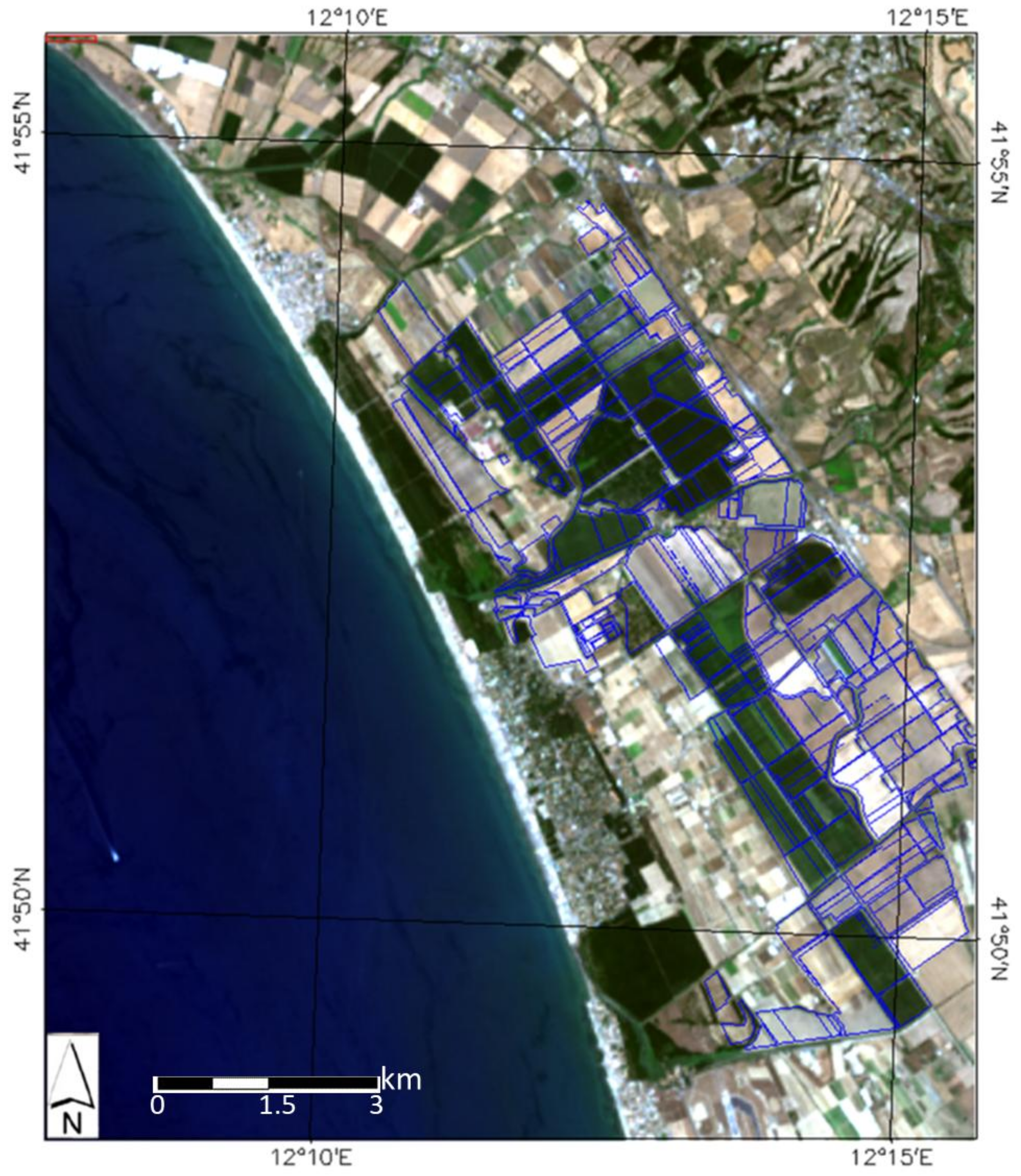
2.1. Study Area and Landsat Dataset

The study area is located in the Maccarese S.p.A. farm (lat. 41°52′18″N, long. 12°14′05″E, alt. 8 m above sea level) near Rome (Central Italy) (Figure 1), within a completely flat agricultural area, originating from land reclamation works carried out in the 1920s. The soil is classified as Cutanic Luvisol [46], with sandy clay loam texture, becoming more clayey towards the northeast of the site. The main crops cultivated in this area are maize, durum wheat, wheat, triticale, barley, carrots and broad beans. These type of crops indicate that there are two main active crop growth seasons in this area, which were considered for this study, from February to April for winter-spring crops, such as wheat, barley, triticale, rapeseed, and broad beans, and from June to August for summer crops, such as maize.
Within the farm, 94 fields of interest (FOI) between 10 and 20 ha were chosen for this study. Figure 1 shows the 94 FOI (in blue color) overlaid on the 08/07/2015 Landsat 8 imagery (R: 655 nm; G: 561 nm; B: 483 nm).
The optical dataset acquired on the study area in Italy is composed of 37 Landsat Enhanced Thematic Mapper Plus (ETM+) (with no data gaps on the FOIs) and 13 Landsat 8 Operational Land Imager (OLI) (GSD 30 m) clear sky (no cloud contamination) images covering all the 94 FOIs, acquired from 2008 to 2015. All the images were spectrally and spatially resampled retaining four spectral bands (blue, green, red, and NIR bands) with a spatial resolution of 30 m and an approximate scene size of 13 km north-south by 11 km east–west. This dataset was used as input in the processing chain for the different clustering procedures, which were applied to produce the constant pattern maps at the field level. It is worth mentioning that crop yield maps collected from 2007 to 2017 were used to compare the capability of the different clustering procedures to detect constant patterns of crop vigor within the selected FOIs. This is because the clusters obtained from satellite time series can be assumed as the representation of different constant potential within each FOI, thus not affected by seasonal fluctuation, and which should match the crop yield patterns for different crop seasons.

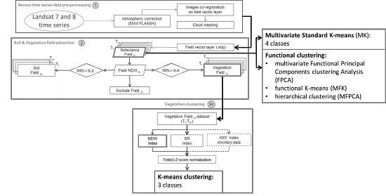
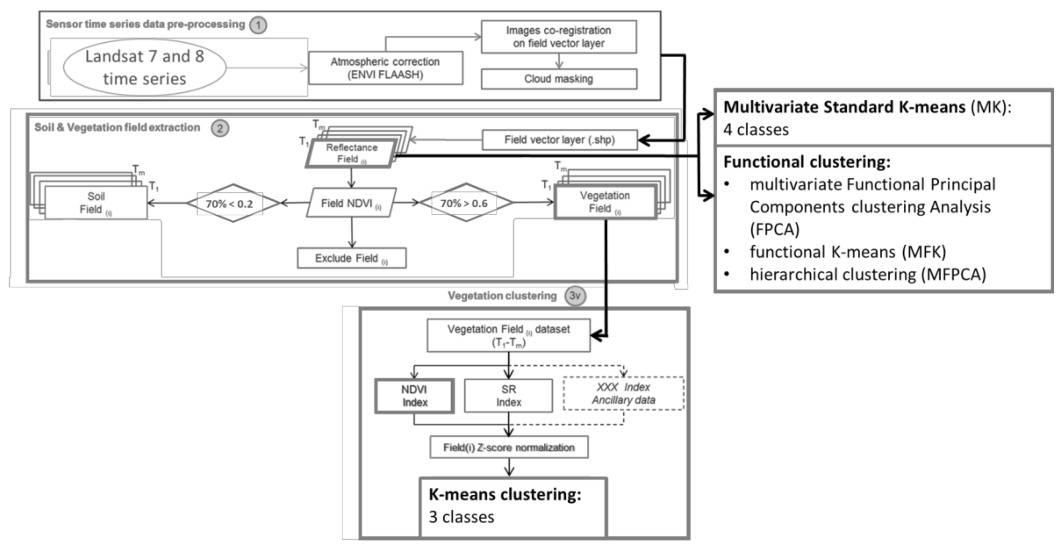
2.2. Landsat Time Series Processing Chain and Standard K-Means Clustering

The methodology, developed in IDL code [47] for processing Landsat time series, consists of three main steps (Figure 2).
The first step involves the setup of the Landsat time series (T1–Tn, i.e., 2008–2015) for further processing. In detail, each image is first atmospherically corrected by using the FLAASH tool based on the MODTRAN4 transfer code implemented in the ENVI image analysis software version 5.0 (Harris Geospatial Solutions, Inc.; Broomfield, CO 80021, United States of America) [47,48]. Next, to ensure an accurate co-registration between the images and the FOI in vector format, each image was spatially resampled (bilinear method) to a higher spatial resolution corresponding to a ground sampling distance (GDS) of 5 m/pixel. The resampling step of the data is just a workaround to assure the correct positioning of the final map with respect to the actual FOI borders.
The second step is devoted to the extraction of the time series (T1–Tm, where m indicates a subset of the n images pertaining to the time series) for each FOI (i), to be clustered in the third step, taking into account that two different datasets, one pertaining to soil and the other one to vegetation, should be extracted. In fact, only images of the active vegetation crop season were considered in this study, for the calculation of vegetation indices and the recognition of related biomass patterns within the same FOI. To this aim, the Normalized Difference Vegetation Index (NDVI), one of the most commonly used vegetation indices for estimating plant “greenness” or photosynthetic activity [49], was calculated for each FOI throughout time:
N D V I = N I R R E D N I R + R E D
where RED means the Landsat sensors’ red band (630–690 nm), while the NIR band is between 760 and 900 nm. The value of this index ranges from −1 to 1. The common range for green vegetation is 0.2 to 0.8 [46]. The selection of a FOI (at a certain date) as pertinent to the soil or vegetation time series was accomplished by calculating the percentage of pixels exceeding a selected threshold on NDVI, and setting another threshold on this percentage. This is done for each FOI over the whole Landsat time series. In particular, for the study area, in order to be sure to identify FOIs occupied by green vegetation, we set a rather high NDVI threshold, i.e., ≥0.6. When NDVI was higher than 0.6 for at least 70% of the pixels of a FOI, at a given acquisition time, the FOI was considered as covered by green vegetation. Conversely, when the NDVI was <0.2 for at least 70% of the pixels, the FOI was considered as occupied by bare soil (or senescent vegetation). This procedure allows to identify, for each image, three types of FOI: (i) green vegetation FOI; (ii) soil FOI; and (iii) mixed FOI. The latter two were excluded from further processing in the present study. It is important to remark that this procedure does not take into account the type of crop (e.g., crop rotation) occurring in the FOI, so that the index trend could include variability related to different FOIs use.
The third processing step consists in the application, to the “Vegetation Fields” layer, of specific indices, suitable to describe the variability at the field scale of the vegetation optical properties (e.g., NDVI, simple ratio index; [49,50]). The standard NDVI was used for this methodology. Furthermore, before applying the clustering procedure, on the NDVI layers, a Z-score spatial normalization [2,51] was used to improve the comparison of spatial patterns occurring within a given FOI, of images acquired on different dates/years. The following equation was used:
Z s c o r e i , j ( t ) = N D V I i , j ( t ) µ j ( t ) σ j ( t )
where NDVIi, j(t) is the value of the NDVI value of the pixel i, field (FOI) j at date t; µj(t) is the mean of the NDVI values of the FOI j at date t; σj(t) is the standard deviation of the NDVI values of the FOI j at date t. By using this normalization, the pixels of each FOI will have zero mean and standard deviation equal to one on each considered date, instead of having NDVI values that depend on the phenological period in which the image was acquired. This should improve the robustness of the identified patterns.
The last step of the procedure consisted of deriving, from the normalized NDVI “Vegetation Field” time series dataset, constant patterns at the field level, by using the standard K-means algorithm, a simple, but effective, commonly-used non-hierarchical clustering algorithm [21].
The K-means algorithm, implemented in IDL programming language (Harris Geospatial Solutions, Inc.; Broomfield, CO 80021, United States of America) [47], calculates initial class means evenly distributed in the data space, and then iteratively clusters the pixels into the nearest class by using a minimum distance method. In each iteration, class means are recalculated and pixels reclassified with respect to the new means, i.e., the within-cluster variation is used as a measure to form homogenous clusters. All the pixels are assigned to the nearest class, unless a standard deviation or distance threshold is specified, in which case some pixels may be left unclassified if they do not meet the selection criteria.
In this study, for the standard K-means classifier applied for this clustering procedure, we fixed a priori (as requested by the algorithm) the number of clusters at three for each FOI. The choice is reasonable taking into account the limited FOIs’ extents (10–20 ha) and their within-field variability. To this aim, for each FOI the average normalized NDVI (temporal series trend) class and the classes above and below the FOI average were calculated.

2.3. Clustering Methods for Multilevel Functional Data

A different clustering approach was also considered for comparison (right part of Figure 2). It uses as the input dataset the atmospherically-corrected and resampled Landsat images (T1–Tn) obtained in the first step of the processing chain described in Section 2.2 (Figure 2). Specifically, for each date in the Landsat time series, the reflectance images corresponding to the four spectral bands centered at 0.482 µm, 0.561 µm, 0.654 µm, and 0.864 µm were extracted. Then, different clustering procedures (described in the following sections) were applied to this multispectral dataset. As is well known, the choice of the optimal number of classes is a crucial issue. Here, we decided to evaluate, for any classification method with a fixed number of classes, the silhouette index [52,53,54], a measure of how the objects are well matched to their own cluster and poorly matched to neighboring clusters. Then, we choose the classification corresponding to the optimum value of the silhouette index for each FOI.
We developed and tested the following functional clustering procedures: (1) standard K-means on multispectral reflectance data; (2) functional K-means; (3) multivariate functional principal components clustering; and (4) hierarchical clustering.

2.3.1. Silhouette Index

Several cluster quality measures, or cluster validity indices, have been proposed in the literature [15]. External indices compare cluster labels to externally supplied class labels (also known as gold standard data or ground truth), whereas internal ones are based solely on cluster similarity. In general, internal measures reward compactness (small distances within clusters) and separation (large distances between clusters). They mainly differ in the way these two aspects are weighted and related, and how sensitive they are to outliers. We chose to adopt the very popular silhouette index because, as thoroughly discussed in [16] where 30 cluster validity indices are compared, “there is a group of about 10 indexes [sic] that seems to be recommendable and Silhouette, Davies-Bouldin and Calinski-Harabasz are in the top of this group”. Moreover, as clearly stated in [55] the silhouette index is less prone to outliers than other internal indices, such as Davies-Bouldin index. The average silhouette width provides an evaluation of clustering validity, and might be used to select an ‘appropriate’ number of clusters [55]. This index is a normalized summation-type index: the compactness, or cohesion, is measured based on the distance between all the points in the same cluster while the separation is measured based on the nearest neighbor distance. For a generic pixel i, we define a(i) as its average distance from the other pixels in its own cluster and b(i) as the minimum among the average distances from the pixels in the other clusters. Then, the silhouette index of pixel i is given by:
s ( i ) = b ( i ) a ( i ) m a x { a ( i ) , b ( i ) } ,
Thus, a s(i) value close to 1 indicates that pixel i is appropriately clustered. The average of the s(i) over all data of a cluster is a measure of how tightly grouped all the data in the cluster are, and the average of s(i) over all data of the entire dataset is a measure of how appropriately the data have been clustered.

2.3.2. Multivariate K-Means (MK)

First of all, we implemented a standard K-means algorithm on the multispectral reflectance time series Yi(t) (with i = 1, 4 in our case), i.e., multivariate data, to check if the algorithm (MK) is capable of distinguishing between bare soil and vegetation, starting from the whole time series of reflectance data, and also to obtain a baseline to assess the improvements due to the introduction of the functional clustering techniques, described in the following subsections. Then, while the clustering methodology is still the traditional K-means, the differences with the algorithm described in Section 2.2 lie in the use of the whole time series, without eliminating images representing non-vegetated periods, and in the representation of each image pixel by four reflectance values at different wavelengths instead of a compact vegetation index, such as the NDVI.

2.3.3. Functional K-Means (MFK)

According to the functional clustering approach, for each pixel the multispectral reflectance time series Yi(t) (with i = 1, 4 in our case) is considered as a discrete sampling of a multidimensional time trajectory, the latter being a realization of a stochastic process Y(t). Such functional data can be represented in finite dimensional space by approximation of the functions in a finite basis (generally, by using B-splines) or by dimension reduction techniques (functional PCA), also in a multilevel/hierarchical framework.
Inspired by the work of [35] we perform a B-spline smoothing of the multivariate data Yi(t) as provided by the R package fda [53], resulting in multivariate smoothed functions Ŷi(t) defined on the whole time interval; to cluster these smoothed functions, the simplest choice is to obtain discrete samples of the Ŷi(t) by evaluating them on an equispaced time grid and then to apply the K-means algorithm to these discrete samples. Several distances can be chosen (e.g., Euclidean, L2, H1), to assess the role of the curves and of their first derivative in distinguishing different clusters. We adopt the L2 distance [53]:
d ( Y ( 1 ) , Y ( 2 ) ) = i T ( Y i ( 1 ) ( t ) Y i ( 2 ) ( t ) ) 2 d t
where Y ^ ( 1 ) , Y ^ ( 2 ) are the multivariate smoothed time series for pixel (1) and (2), respectively, with the subscript i denoting their components; the integral is to be evaluated on the whole time interval T or on its discretization on the equispaced grid mentioned above.

2.3.4. Multivariate Functional Clustering (FPCA)

We also implemented a multivariate FPCA, based on the approach proposed by [42]. Classical multivariate FPCA concatenates the multiple functions into one, to perform univariate FPCA. This method should perform well on the considered dataset, since the components of multivariate functional data are measured in the same units and have similar variation. However, normalization can also be considered in the FPCA in order to account for differences in degrees of variability and in quantity among the components of the multivariate random functions. Specifically, we truncate the Karhunen Loeve expansion of the multidimensional smoothed functions Ŷi(t) at the first q terms and cluster on the principal component scores. Thus, FPCA reduces high-dimensional functional data into low-dimensional principal component score vectors, while retaining most information: the number of components kept, q, is such that the cumulative percentage of variance explained is greater than 0.9. Then, clustering is applied to the estimated scores.

2.3.5. Hierarchical Clustering (MFPCA)

Hierarchical clustering is a well-acknowledged methodology consisting of a series of partitions, obtained proceeding by successive fusions of subjects (agglomerative clustering) or successive separations (divisive clustering). In such a broad field, the multilevel functional PCA (MFPCA, [45]) was specifically designed for multilevel functional data, i.e., data with a natural hierarchy, for example multiple recordings of the same subject. Since the covariance of such data has a multilevel structure, this method is able to decompose the total functional variation into between-subject and within-subject variation via the functional analysis of variance. Then it can capture dominant modes of variations and reduce dimensions by conducting FPCA at both levels. Specifically, we implemented the hierarchical clustering proposed in [41] assuming two levels in our data.
We state that level 1 clustering refers to the average behavior across all dimensions, whereas level 2 clustering is related to dimension-specific behaviors. At level 1, two units are in the same cluster if their unit-specific means are similar in shape; while at level 2, two units are in the same cluster if their corresponding deviations from the unit-specific means are dynamically similar or they move together over time. Again, MFPCA reduces high-dimensional functional data into low dimensional principal component score vectors: at each level, only a few components are kept and clustering is applied to the estimated scores at this level. Obviously, all these procedures depend on the fixed number of K clusters. In this case study we chose K = 4, by constraining the procedure to distinguish bare soil (one cluster) from vegetation and, within vegetated FOIs, to discriminate, as for the standard K-means algorithm, three clusters representing different levels of crop vigor (mean class, above the mean, and below the mean).

2.4. Clustering Accuracy Assessment

The clustering accuracy assessment is not a trivial task, for example internal cluster validity indices could not be used—as they are part of the clustering procedure in most of the approaches, and external validity indices could not be applicable too. In fact, external validity indices ask for ground truth, which, in this circumstance, could not be found. The reason lies in the fact that clustering results, though very useful for crop management, do not represent an observable or measurable entity with an evidence—such as land cover or leaf chlorophyll content—it is a notional category, theoretically indicative of long-term yield potential/trend pattern. This is the reason why, taking into account this hypothetical relation, yield maps were used as an indirect representation of the desired output. This has to be considered an indirect information since: (i) yield is related not only to crop limiting factors, but also to agro-practices; and (ii) yield is affected by seasonality and the maps are available just for few years, making it difficult to generalize such data to long-term potential.
Therefore, the reliability of the clustering methods, for the assessment of within-field patterns of crop productivity, was tested in this work by using crop yield maps for fourteen FOIs of the Maccarese S.p.A. farm. In four FOIs, the yield maps were available for two years (FOI 10, 13, 24 and 54), whereas in all the others yield maps were only available for one year, resulting in eighteen validation test cases. Wheat yield data/maps between 2007 and 2017 were collected by a combine harvester equipped with a differential global position system (DGPS) and a grain flow sensor, providing spatially referenced yield data [56,57,58]. The raw yield data were refined by removing yield values obtained at the edge of the FOI, or in case the harvester cutting width was incorrectly set, or for those values collected when the combine harvester was on a low speed or without differential GPS data.
The refined yield data were used to evaluate if there are significant differences in yield between areas classified by the clustering methods. For this comparison we used the polygon kriging method [42], which allows to take into account the spatial correlation in the FOI, hence obtaining for each cluster (an irregularly shaped polygon) a spatially weighted average estimate (the expected value) and the standard deviation of the yield [49,50]. The polygon kriging method is similar to block kriging, but the former is applied to an irregular polygon, discretized into regular cells, instead of a square block. The average covariance function for each polygon is obtained by the computation of a weighted discrete summation of the point covariance function, where the weights are based on the proportion of the cell inside the polygon [45]. The differences between clusters (polygons) were determined by observing the expected values and their 99% confidence intervals (lower and upper limit) for each polygon.
We compared the different clustering methods observing the optimum number of clusters for each FOI assuming that this optimum corresponds to the maximum number of clusters detected among all the clustering methods, which are also statistically different in terms of crop yield.

3. Results

3.1. Clustering Results

3.1.1. Standard K-Means Clustering Results

The results obtained by applying the standard K-means clustering algorithm using as input the concatenated images extracted from the Landsat images time series (i.e., the vegetation field (i) dataset (T1–Tm) in Figure 2), are presented in Figure 3a. For comparison, the results of the hierarchical MFPCA (Figure 3b), as applied on the spectral reflectance time series, is also shown. The choice is justified by the fact both methods rely on a fixed number of clusters for each FOI to be defined in advance: three clusters for the standard K-means and four clusters for the MFPCA.
The results obtained for the biomass clustering for each investigated FOI do not show temporally-structured results, since the K-means algorithm is not able to identify specific temporal behaviors, but just similar spatial behavior for each FOI across Landsat time series. It is evident from Figure 3 that although in some fields there is a general agreement between the results of the two clustering algorithms, in the identification of areas with crop vigor higher (or lower) than the average; in many cases the results are rather different.

3.1.2. Functional Clustering Results

All the clustering procedures from Section 2.3 have been applied to the complete Landsat spectral reflectance time series, as described in Section 2.1, after the atmospheric correction and spatial resampling of the images.
The clustering maps for each procedure have been produced and the MK, MFK, and FPCA functional clustering maps are presented in Figure 4, while maps obtained from MFPCA are presented in Figure 3b. In these figures, in order to simplify the comparison of the results, we choose to adopt a color scale ranging from red to green. Such a color scale was determined by post-clustering evaluation of the NDVI mean value of each cluster and a subsequent ordering of the clusters from the lowest (red) to the highest (green) NDVI. It should be stressed that NDVI was not used within the clustering algorithms, but just as a post-clustering for labelling purposes. For each procedure, the optimal number of clusters, according to the related mean silhouette index, is generally very low: for two thirds of the considered FOIs this number is two or three (specifically, 60 FOIs for MK, 65 FOIs for MFK and 68 FOIs for FPCA). Only for a few specific FOIs all the procedures suggest a higher number of clusters: for 11 fields the estimated optimal number of clusters is six, or higher. In general, FOIs borders are not identified as a single cluster. However, some spatial structures in the vegetation, such as stripes parallel to the FOI borders, are often highlighted and detected.

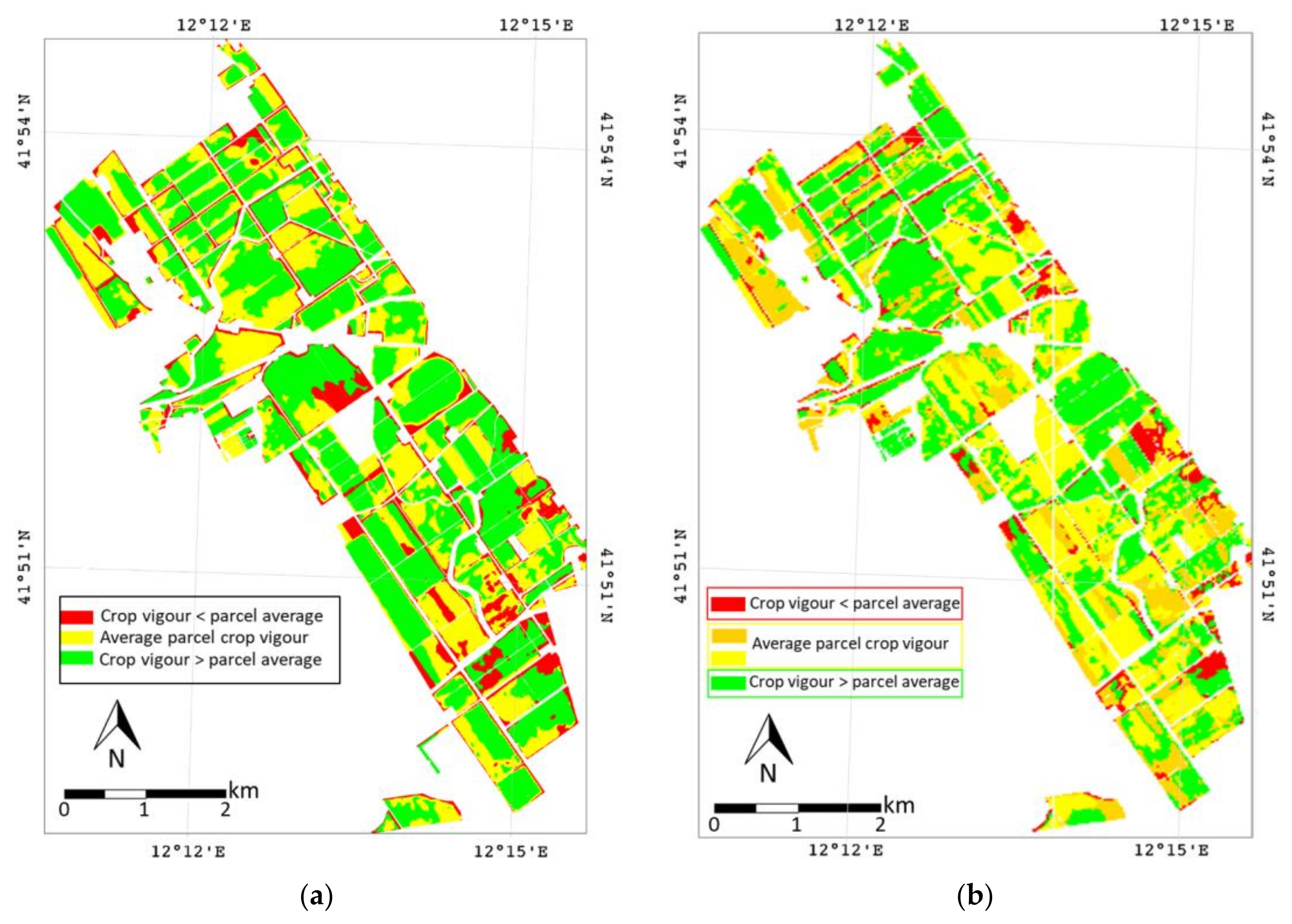
3.2. Ability of Clustering Methods to Capture Actual Yield Patterns

The differences between each cluster (polygon) of the validation FOIs were statistically evaluated taking into account the expected yield values obtained applying the polygon kriging on the 14 validation FOIs. The number of classes was set in advance for K-means (3 classes) and MFPCA (four classes). The classes identified by the two methods were significantly different in 16 validation tests for K-means and in 15 cases for MFPCA (Table 1). The other three clustering methods (FPCA, MK, and MFK) did not provide a constant number of classes. The number of detected and significantly different classes was the same for thirteen validation tests, both using MK and MFK methods, whereas using the FPCA method the number of significantly different classes matched the number of detected classes 16 times (Table 1).
We remark that “optimal” (OPT in Table 1) means here the maximum number of statistically different clusters that can be identified across all the considered methods. This is assessed by considering as optimal the highest number of clusters, but only after statistical verification that these clusters correspond to significant differences in yield maps. As Table 1 shows, in the fourteen validation FOIs, this number (last column in Table 1, OPT) ranges from two to eight, so that the methods that do not fix the clusters number in advance (i.e., FPCA, MK, and MFK) are clearly to be preferred. Indeed, while it is reasonable to generally assume three or four clusters, the data can suggest different scenarios on different FOIs.
Examining the validation results, the lowest class in terms of crop vigor is always localized close to the FOI edges when using the K-means method (Figure 3), except for some FOIs in the southern part of the Maccarese farm. For the other clustering approaches, where the number of classes was not set in advance, the low class (crop vigor less than field average) is not confined to the FOIs’ boundaries, and there are many FOIs where only two classes were detected (average field crop vigor and crop vigor higher than the field average). Consequently, the “low” class is not present (Figure 4). The MFK method, in comparison to the FPCA, seems to provide a spatial distribution more in agreement with the K-means, even though the results provided by MFK are more detailed, i.e., this method provided the best results in terms of “optimal” number of statistically different clusters retrieved. In fact, the number of statistically different clusters for the MFK method is often very close to the optimal number (Table 1).
As an example, to give an agronomical insight into the meaning of the clusters, we showed the comparison between recorded yield maps and the clusters detected by the five methods in six FOIs (Figure 5).
The yield map of the FOI 24 shows lower productivity in the northeastern, southwestern, and central parts of the FOI (Figure 5). The K-means method reflects the spatial distribution of the wheat yield, especially at the FOI boundaries, however, both MFK and MK methods identified the highest number of significantly different classes (Figure 6). In particular, MFK allowed to identify six clusters consistent with the yield map and statistically different among them (Figure 5 and Figure 6). The brown (cluster 2) and red (cluster 3) areas, respectively showed an expected value of 4.2 and 3.7 t·ha−1, and these values are consistent with measured yields values within these clusters (ranging from 1.9 to 5.3 t·ha−1). The yellow cluster is characterized by an expected value of 4.6 t·ha−1, a value very close to the measured mean value within the FOI (4.8 t·ha−1). The three green areas, in the northern and southern parts of the FOI, actually detected regions having the highest measured yield values. The other two clustering methods showed different problems: FPCA detected only three classes that do not describe all the spatial variability of the FOI, especially in the southern part of the FOI, while the clustering obtained by MFPCA did not match up well with the yield map.
Although the recorded yield values are very low in the FOI 30, this FOI is clearly divided into two main parts: high productivity in the northeast part, where the average measured yield value is 4.5 t·ha−1, and low productivity in the southwest, showing an average yield value of 1.9 t·ha−1 (Figure 5). The FPCA, MK, and MFK methods provided very similar results: only two clusters that are consistent with the two abovementioned yield patterns. The two classes detected by MFK showed an expected value of 2 t·ha−1 for the yellow cluster and 4.6 t·ha−1 for the green one, while for the FPCA and MK both the expected values of the two clusters are slightly higher than those estimated using MFK. The K-means identified a third cluster at the edges, but although all the clusters are significantly different, the expected yield values of the medium and high class are very similar: 3.3 and 3.4 t·ha−1, respectively. The four classes detected by MFPCA seem inadequate, in particular, the two lowest classes are not significantly different between them and both have a very small dimension (Figure 5).
In the FOI 36, low yield zones are localized in the southwest and northeast (yield: 0.88–2.0 t·ha−1), while in the central area higher yield values were registered (3.2–6.8 t·ha−1). This spatial distribution is well described by the MFK, FPCA, and K-means clusters. However, the two low-productivity clusters of MFK and FPCA are not statistically different. The MFPCA method was able to distinguish four classes showing a reasonable visual match with the yield map, even if the lowest three classes are very close among them.
The optimal number of clusters in the FOI 27 is four; both MK and MFK methods provided the best correspondence between yield patterns and clusters (Figure 5). However, the clusters detected by K-means method also show a clear link with measured yield values, while the two other methods (FPCA and MFPCA) were not able to display the within-field variability. Observing the yield map, a low yield area can be clearly observed at the northern edge of the field that corresponds to cluster 1 of the MK and K-means methods. This cluster is adjacent to an area showing higher yield values, which matches cluster 3 of MK, MFK, and K-means methods, where the expected value for the three methods ranges between 4.3 (MFK) and 5.0 (MK and K-means) t·ha−1. The southern part of the field is more productive, especially in the southwest section, which corresponds to cluster 2 for MK (6.1 t·ha−1) and cluster 1 for MFK (6.2 t·ha−1).
FOI 64 is a very large field, composed of many parcels, thus, the optimal number of clusters is quite high and it was detected by the MK method. The other clustering approaches underestimate the field variability, in particular FPCA, which provided only two clusters and MFPCA, which identified four classes, but only two have a relevant extension (Figure 5). The yield map of FOI 64 shows a narrow belt in the central area having low yield values, which were included in cluster 4 of MK (expected value 4.7 t·ha−1). In the southeast part of FOI 64 the highest yield values can be observed (average value of 11.5 t·ha−1), which correspond to clusters 5 and 6 of MK, having, respectively, an expected value of 13.4 and 10.7 t·ha−1.
FOI 77 consists of two large parcels, which show different productivity levels: high yield values in the southwest part (mean yield value of 7.8 t·ha−1) and low and medium values in the northeast part of the FOI (mean yield value of 4.7 t·ha−1). The optimal number of clusters of this FOI is five, which was obtained by the MK and MFK methods. However, clusters 1, 4, and 5 obtained by the MK method have very similar expected values, which range between 6.3 and 6.5 t·ha−1. Cluster 2 of MK and cluster 4 of MFK match the area with low productivity in the northeast part of the field, where the measured yield values range between 1 and 5 t·ha−1. In this low productivity cluster the expected yield values are 3.1 for MK and 3.3 t·ha−1 for MFK. The other clustering methods provided few clusters, which do not match the spatial variability displayed by the yield map.

4. Discussion

The present study illustrates the potential of the proposed clustering methodologies for applications in the area of precision land management. In this context, the identification of the most suitable methodologies for capturing the stable patterns underlying the spatial variability observed in soil and vegetation variables is a very active research area. Most of the approaches that have been proposed rely on complex multivariate geostatistical techniques of data fusion of ground-based data, e.g., from geophysical [56,59] and proximal sensors [13,14], which are not always available with remote sensing data. Therefore, there is a great interest in the development of methodologies relying only on remote sensing data, which could be rapidly developed into high-level spatial products delivered to land managers. However, in order to be trusted by users, the validity of the methodologies proposed for the identification of stable, clear, and manageable zones within a field needs to be assessed. This is always rather difficult, since the observed spatial variability is superimposed onto a generally even higher temporal variability. Additionally, the validity of the identification of uniform zones has to be considered in relation to the objectives of the user, e.g., choosing classes of uniform management.
In the literature there are several sophisticated clustering methods based on spectral clustering algorithms that are used for different applications such as those proposed by [27,28,29]. However, in the present work, we chose, as an objective assessment variable of the goodness of the compared clustering methodologies, the ability to identify from multispectral satellite time series statistically significant yield differences among the clusters. Now, the application of spectral clustering or diffusion learning algorithms to remote satellite time series is quite rare in the literature. The main reason, in our opinion, is that these methods are not well suited for handling sequential information, so that the risk is to disregard the time structure of data while clustering. Moreover, the computational cost of algorithms such as spectral clustering is sensibly higher than both the standard K-means and functional clustering. Our approach assumes a functional model for the data at hand (a time series of multispectral images). Such functions represent the trajectories of a stochastic process and the clustering is performed on the whole curves, or on a suitable parameterization of them. Then, the observations are supposed to be a finite sample of points extracted from these curves, which belong to an infinite dimensional space. To efficiently represent such curves, we adopt the coefficients of their basis expansion, as in the MFK method (where the dimension depends on the chosen number of basis functions), or also their principal components scores for the FPCA method. Both these two last methods reduce the dimension of the clustering problem: as a comparison, in the MK method, the dimension of the data is given by the length of the time series times the number of considered wavelengths. That dimension for our dataset is about 200.
Clustering methodologies results obtained for the chosen agricultural area in Italy using Landsat multispectral satellite time series as input can be summarized and discussed as follows: The standard K-means clustering, applied to NDVI Landsat time series in the first procedure, proposed in Section 2.2, generally seems to retrieve a cluster dimension and distribution that are in accordance with the FOI’s dimension and crop yield within-field spatial distribution of the study area. Although the K-means classes and the yield maps often match, setting the number of classes to three could be restrictive in large fields (e.g., see FOI 36 in Figure 5) and excessive in small fields (e.g., see FOI 30 in Figure 5). On the other hand, multivariate K-means (MK) is theoretically very similar to the standard K-means, but it was applied to the spectral reflectance Landsat time series and, therefore, not only related to the difference between near-infrared and red light (i.e., NDVI). Moreover, this method has the potential to exploit the information yielded by the whole multispectral signal (Landsat bands). In our experiments, the clustering differences between standard K-means and MK are mainly due to the freedom in the choice of the number of clusters. On the other hand, the MFK and FPCA clustering methodologies take a great advantage from the functional approach: data are smoothed and their dimension reduced before clustering. Consequently, these procedures are weakly affected by irregularities in the time series. MFPCA seemed to be a promising approach, because of the hierarchical nature of the information to be retrieved, i.e., a large spectral difference between bare soil and vegetation and a smaller difference among the different crop yield in the FOIs. However, the procedure is still to be refined and it is quite sensitive to the irregular temporal resolution of the time series of images; the clustering results on the considered dataset are definitely not satisfying with respect to the yield maps.
In general, as clearly reported in the Results section, the clustering approaches that do not require setting the number of cluster in advance (i.e., MK, MFK, and FPCA), have proved to be more suitable to describe the within-field variability as compared to the other methods (standard K-means and MFPCA). It has to be noted that the silhouette index, applied here to choose the optimal number of clusters, while being undoubtedly a reasonable proposal, has not always provided good results. Specifically, when applied to the FPCA method, it often suggested just two clusters, even in very large FOIs. The individuation of a priori criteria for determining the optimal number of clusters remains then, in our opinion, an open issue.
Another point to be stated is that functional clustering methods have shown to be able to detect constant patterns in time series data and to identify statistically different clusters in the reported experiments. Among these methods, MFK has shown the best performance, both in terms of statistical significance of the different clusters detected in the analyzed FOIs and in terms of clustering accuracy as evaluated by consistency with the yield maps used for validation. Another advantage of MFK clustering methodology is its ease of implementation and low computational cost with respect to other approaches mentioned in the Introduction section.

5. Conclusions

In this study, the capability of different clustering procedures in mapping constant patterns, at the field level, using as input multispectral satellite data, and, in particular, by the use of multivariate functional clustering for remote sensing time series data, has been assessed. Archived Landsat 7 and 8 time series have been considered to this aim. Crop yield maps collected from 2007 to 2017 have been used to assess the capability of each applied clustering procedure to detect constant patterns related to within-field crop vigor.
The main conclusion of our study is that the MK, MFK, and FPCA clustering approaches, which do not require setting the number of clusters in advance, are more suitable to describe the within-field variability as compared to the other methods (standard K-means and MFPCA).
In particular, functional clustering methods demonstrated: (i) as concerns the temporal dimension, to be less prone to the seasonal noise, and to be able to capture the long term signal, which is the information of interest; and (ii) as regards the spatial dimension, to be suitable to detect constant patterns in satellite time series identifying the optimal number (OPT values in Table 1) of clusters, with a good match with the yield maps’ patterns.
The MFPCA is an exception, as it appears to be quite sensitive to the uneven temporal distribution of satellite acquisitions, and since it asks for an a priori definition of the number of classes.
In fact, the possibility of adaptively choosing the number of clusters proved to be crucial. This is grounded in the fact that the differences in the granularity of field variability, as observed in the real parcels, are great, even in neighboring ones. Nevertheless, the selection of a priori criteria for determining the optimal number of clusters (in this study the silhouette index) remains, in our opinion, an open issue to be addressed in the future.
In conclusion, on the basis of the obtained results, the usefulness of multivariate functional clustering for the analysis of remote sensing time series for agricultural studies has been proved.
Among the compared approaches, MFK has shown to outperform the other methods, both in terms of statistical significance of the identified clusters—within the single FOIs, and of clustering accuracy—as evaluated by consistency with the yield maps used for validation. Moreover, MFK, with respect to other approaches, offers faster implementation and lower computational costs.
Future research will be advantaged by the free availability of a large amount of satellite time series data, such as Sentinel 2A,B (European Space Agency) multispectral data, which have operated simultaneously since 2017 (with a revisit time of five days and spatial resolution of 10–20 m).
In view of the results obtained by using Landsat bands for the MFK algorithm, instead of a spectral index involving two bands in the VNIR as for the standard K-means algorithm, current multispectral (Sentinel and Landsat 8) and future hyperspectral satellite sensors (e.g., PRISMA, GF-5, EnMAP, ECOSTRESS, VENµS, and Sentinel 10; [60]) will provide a further improvement in clustering methods and performance. The availability of new data with increased spatial, temporal and spectral resolution will certainly require further experiments on these clustering procedures to more robustly assess their performance.

Acknowledgments

The research leading to these results has received funding from the European Union Seventh Framework Programme (FP7/2007–2013) under grant agreement no. 606983 (ERMES project). This research was also carried out in the framework of the Smart Basilicata (contract no. 6386—3, 20 July 2016) which was approved by the Italian Ministry of Education, University and Research (Notice MIUR n.84/Ric 2012, PON 2007–2013 of 2 March 2012) and was funded with the Cohesion Fund 2007–2013 of the Basilicata Regional authority. The authors would like to thank the personnel of the Maccarese Spa farm for providing the yield maps.

Author Contributions

All co-authors of this manuscript significantly contributed to all phases of the investigation. They contributed equally to the preparation, analysis, review, and editing of this manuscript.

Conflicts of Interest

The authors declare no conflict of interest.

References

  1. Blasch, G.; Spengler, D.; Hohmann, C.; Neumann, C.; Itzerott, S.; Kaufmann, H. Multitemporal soil pattern analysis with multispectral remote sensing data at the field-scale. Comput. Electron. Agric. 2015, 113, 1–13. [Google Scholar] [CrossRef]
  2. Huang, C.; Goward, S.N.; Masek, J.G.; Thomas, N.; Zhu, Z.; Vogelmann, J.E. An automated approach for reconstructing recent forest disturbance history using dense landsat time series stacks. Remote Sens. Environ. 2010, 114, 183–198. [Google Scholar] [CrossRef]
  3. Verbesselt, J.; Hyndman, R.; Newnham, G.; Culvenor, D. Detecting trend and seasonal changes in satellite image time series. Remote Sens. Environ. 2010, 114, 106–115. [Google Scholar] [CrossRef]
  4. FARMSTAR. Available online: http://www.farmstar-conseil.fr/ (accessed on 5 August 2017).
  5. ERMES (an Earth obseRvation Model Based ricE Information Service). Available online: http://www.ermes-fp7space.eu/en/about-ermes/ (accessed on 1 October 2017).
  6. Ge, Y.; Thomasson, J.A.; Sui, R. Remote sensing of soil properties in precision agriculture: A review. Front. Earth Sci. 2011, 5, 229–238. [Google Scholar] [CrossRef]
  7. Blasch, G.; Spengler, D.; Itzerott, S.; Wessolek, G. Organic matter modeling at the landscape scale based on multitemporal soil pattern analysis using RapidEye data. Remote Sens. 2015, 7, 11125–11150. [Google Scholar] [CrossRef]
  8. Mulla, D.J. Twenty five years of remote sensing in precision agriculture: Key advances and remaining knowledge gaps. Biosyst. Eng. 2013, 114, 358–371. [Google Scholar] [CrossRef]
  9. Eerens, H.; Haesen, D.; Rembold, F.; Urbano, F.; Tote, C.; Bydekerke, L. Image time series processing for agriculture monitoring. Environ. Model. Softw. 2014, 53, 154–162. [Google Scholar] [CrossRef]
  10. Bellón, B.; Bégué, A.; Lo Seen, D.; de Almeida, C.A.; Simões, M. A remote sensing approach for regional-scale mapping of agricultural land-use systems based on NDVI time series. Remote Sens. 2017, 9, 600. [Google Scholar] [CrossRef]
  11. Baruth, B.; Royer, A.; Klisch, A.; Genovese, A. The Use of Remote Sensing within the MARS Crop Yield Monitoring System of the European Commission; ISPRS, Commission VIII: Stresa, Italy, 2008; pp. 935–941. [Google Scholar]
  12. Becker-Reshef, I.; Justice, C.; Sullivan, M.; Vermote, E.; Tucker, C.; Anyamba, A.; Small, J.; Pak, E.; Masuoka, E.; Schmaltz, J.; et al. Monitoring global croplands with coarse resolution earth observations: The Global Agriculture Monitoring (GLAM) Project. Remote Sens. 2010, 2, 1589–1609. [Google Scholar] [CrossRef]
  13. Casa, R.; Castrignanò, A. Analysis of spatial relationships between soil and crop variables in a durum wheat field using a multivariate geostatistical approach. Eur. J. Agron. 2008, 28, 331–342. [Google Scholar] [CrossRef] [Green Version]
  14. Castrignanò, A.; Buttafuoco, G.; Quarto, R.; Vitti, C.; Langella, G.; Terribile, F.; Venezia, A. A combined approach of sensor data fusion and multivariate geostatistics for delineation of homogeneous zones in an agricultural field. Sensors 2017, 17, 2794. [Google Scholar] [CrossRef] [PubMed]
  15. Tibshirani, R.; Walther, G.; Hastie, T. Estimating the number of clusters in a data set via the gap statistic. J. Roy. Statist. Soc. B 2001, 63, 411–423. Available online: http://www.web.stanford.edu/~hastie/Papers/gap.pdf (accessed on 18 October 2016). [CrossRef]
  16. Rousseeuw, P.J. Silhouettes: A graphical aid to the interpretation and validation of cluster analysis. J. Comput. Appl. Math. 1987, 20, 53–65. [Google Scholar] [CrossRef]
  17. Arbelaitz, O.; Gurrutxaga, I.; Muguerza, J.; Pérez, J.M.; Perona, I. An extensive comparative study of cluster validity indexes. Pattern Recognit. 2013, 46, 243–256. [Google Scholar] [CrossRef]
  18. Lozano, J.A.; Pena, J.M.; Larranaga, P. An empirical comparison of four initialization methods for the K-means algorithm. Pattern Recognit. Lett. 1999, 20, 1027–1040. [Google Scholar] [CrossRef]
  19. Zaady, E.; Karnieli, A.; Shachak, M. Applying a field spectroscopy technique for assessing successional trends of biological soil crusts in a semi-arid environment. J. Arid Environ. 2007, 70, 463–477. [Google Scholar] [CrossRef]
  20. Jain, A.K.; Flynn, P.J. Image segmentation using clustering. In Advances in Image Understanding; Wiley-IEEE Computer Society Press: Washington, DC, USA, 1996; pp. 65–83. [Google Scholar] [CrossRef]
  21. Jain, A.K. Data clustering: 50 years beyond K-means. Pattern Recognit. Lett. 2010, 31, 651–666. [Google Scholar] [CrossRef]
  22. Richards, J.W.; Hardin, J.; Grosfils, E.B. Weighted model-based clustering for remote sensing image analysis. Comput. Geosci. 2010, 14, 125–136. [Google Scholar] [CrossRef]
  23. Ma, A.; Zhong, Y.; Zhang, L. Spectral-Spatial Clustering with a Local Weight Parameter Determination Method for Remote Sensing Imagery. Remote Sens. 2016, 8, 124. [Google Scholar] [CrossRef]
  24. Choubin, B.; Solaimani, K.; Habibnejad Roshan, M.; Malekian, A. Watershed classification by remote sensing indexes: A fuzzy c-means clustering approach. J. Mt. Sci. 2017, 14, 2053. [Google Scholar] [CrossRef]
  25. Ng, A.; Jordan, M.; Weiss, Y. On spectral clustering: Analysis and an algorithm. In Advances in Neural Information Processing Systems; Dietterich, T., Becker, S., Ghahramani, Z., Eds.; MIT Press: Cambridge, UK, 2002; Volume 14, pp. 849–856. [Google Scholar]
  26. Von Luxburg, U. A tutorial on spectral clustering. Stat. Comput. 2007, 17, 395–416. [Google Scholar] [CrossRef]
  27. Rodriguez, A.; Laio, A. Clustering by fast search and find of density peaks. Science 2014, 344, 1492–1496. [Google Scholar] [CrossRef] [PubMed]
  28. Elhamifar, E.; Vidal, R. Sparse manifold clustering and embedding. Adv. Neural Inf. Process. Syst. 2011, 24, 55–63. [Google Scholar]
  29. Murphy, J.M.; Maggioni, M. Nonlinear Unsupervised Clustering of Hyperspectral Images with Applications to Anomaly Detection and Active Learning, Computer Science—Computer Vision and Pattern Recognition. arXiv, 2017; arXiv:1704.07961. [Google Scholar]
  30. Little, A.; Maggioni, M.; Murphy, J.M. Path-Based Spectral Clustering: Guarantees, Robustness to Outliers, and Fast Algorithms. arXiv, 2017; arXiv:1712.06206. [Google Scholar]
  31. Little, A.; Byrd, A. A Multiscale Spectral Method for Learning Number of Clusters. In Proceedings of the 2015 IEEE 14th International Conference on Machine Learning and Applications (ICMLA), Miami, FL, USA, 9–11 December 2015. [Google Scholar]
  32. Jebara, T.; Song, Y.; Thadani, K. Spectral Clustering and Embedding with Hidden Markov Models. In Machine Learning: ECML 2007. ECML 2007. Lecture Notes in Computer Science; Kok, J.N., Koronacki, J., Mantaras, R.L., Matwin, S., Mladenič, D., Skowron, A., Eds.; Springer: Berlin/Heidelberg, Germany, 2017; Volume 4701. [Google Scholar]
  33. Jacques, J.; Preda, C. Functional data clustering: A survey. Adv. Data Anal. Classif. 2014, 8, 231–255. [Google Scholar] [CrossRef]
  34. Ieva, F.; Paganoni, A.M.; Pigoli, D.; Vitelli, V. Multivariate functional clustering for the morphological analysis of electrocardiograph curves. J. R. Stat. Soc. Ser. C 2013, 62, 401–418. [Google Scholar] [CrossRef]
  35. Serban, N.; Jiang, H. Multilevel Functional Clustering Analysis. Biometrics 2012, 68, 805–814. [Google Scholar] [CrossRef] [PubMed]
  36. Li, H.; Deng, X.; Dolloff, C.A.; Smith, E.P. Bivariate functional data clustering: Grouping streams based on a varying coefficient model of the stream water and air temperature relationship. Environmetrics 2015, 27, 15–26. [Google Scholar] [CrossRef]
  37. Romano, E.; Mateu, J.; Giraldo, R. On the performance of two clustering methods for spatial functional data. Adv. Stat. Anal. 2015, 99, 467–492. [Google Scholar] [CrossRef]
  38. Gaetan, C.; Girardi, P.; Pastres, R. Spatial clustering of curves with an application of satellite data. Spat. Stat. 2017, 20, 110–124. [Google Scholar]
  39. Haggarty, R.; Miller, C.M.; Scott, E.; Wyllie, F.; Smith, M. Functional clustering of water quality data in Scotland. Environmetrics 2012, 23, 685–695. [Google Scholar] [CrossRef]
  40. Luz-López-García, M.; García-Ródenas, R.; González-Gómez, A. K-means algorithms for functional data. Neurocomputing 2015, 151, 231–245. [Google Scholar] [CrossRef]
  41. Berrendero, J.R.; Justel, A.; Svarc, M. Principal components for multivariate functional data. Comput. Stat. Data Anal. 2011, 55, 2619–2634. [Google Scholar] [CrossRef]
  42. Di, C.Z.; Crainiceanu, C.M.; Caffo, B.S.; Punjabi, N.M. Multilevel functional principal component analysis. Ann. Appl. Stat. 2009, 3, 458–488. [Google Scholar] [CrossRef] [PubMed]
  43. Nguyen, C.; Starek, M.J.; Tissot, P.; Gibeaut, J. Unsupervised Clustering Method for Complexity Reduction of Terrestrial Lidar Data in Marshes. Remote Sens. 2018, 10, 133. [Google Scholar] [CrossRef]
  44. Tu, W.; Hu, Z.; Li, L.; Cao, J.; Jiang, J.; Li, Q.; Li, Q. Portraying Urban Functional Zones by Coupling Remote Sensing Imagery and Human Sensing Data. Remote Sens. 2018, 10, 141. [Google Scholar] [CrossRef]
  45. Goovaerts, P. Kriging and semivariogram deconvolution in the presence of irregular geographical units. Math. Geosci. 2008, 40, 101–128. [Google Scholar] [CrossRef]
  46. FAO-ISRIC-ISSS. World Reference Base for Soil Resources; World Soil Resources Report 84; Food and Agriculture Organization: Rome, Italy, 1998. [Google Scholar]
  47. ENVI/IDL Scientific Programming Language. Available online: http://www.envi geospatial.com/ProductsandSolutions/GeospatialProducts/IDL.aspx (accessed on 10 October 2016).
  48. Matthew, M.W.; Adler-Golden, S.M.; Berk, A.; Richtsmeier, S.C.; Levine, R.Y.; Bernstein, L.S.; Acharya, P.K.; Anderson, G.P.; Felde, G.W.; Hoke, M.P.; et al. Status of Atmospheric Correction Using a MODTRAN4-based Algorithm. In SPIE Proceedings, Algorithms for Multispectral, Hyperspectral, and Ultraspectral Imagery VI; AeroSense 2000: Orlando, FL, USA, 2000; Volume 4049, pp. 199–207. [Google Scholar]
  49. Yengoh, G.T.; Dent, D.; Olsson, L.; Tengberg, A.E.; Tucker, C.J., III. Use of the Normalized Difference Vegetation Index (NDVI) to Assess Land Degradation at Multiple Scales; Springer Briefs in Environmental Science; Springer International Publishing: Berlin, Germany, 2016; pp. 1–110. [Google Scholar]
  50. Reichenau, T.G.; Korres, W.; Montzka, C.; Fiener, P.; Wilken, F.; Stadler, A.; Waldhoff, G.; Schneider, K. Spatial Heterogeneity of Leaf Area Index (LAI) and Its Temporal Course on Arable Land: Combining Field Measurements, Remote Sensing and Simulation in a Comprehensive Data Analysis Approach (CDAA). PLoS ONE 2016, 11, e0158451. [Google Scholar] [CrossRef] [PubMed]
  51. Zhu, Z.; Woodcock, C.E.; Olofsson, P. Continuous monitoring of forest disturbance using all available Landsat imagery. Remote Sens. Environ. 2012, 122, 75–91. [Google Scholar] [CrossRef]
  52. De Amorim, R.C.; Hennig, C. Recovering the number of clusters in data sets with noise features using feature rescaling factors. Inf. Sci. 2015, 324, 126–145. [Google Scholar] [CrossRef] [Green Version]
  53. R. Package Fda. Available online: https://cran.r-project.org/web/packages/fda/fda.pdf (accessed on 10 October 2017).
  54. Castaldi, F.; Casa, R.; Pelosi, F.; Yang, H. Influence of acquisition time and resolution on wheat yield estimation at the field scale from canopy biophysical variables retrieved from SPOT satellite data. Int. J. Remote Sens. 2015, 36, 2438–2459. [Google Scholar] [CrossRef]
  55. Wiwie, C.; Baumbach, J.; Röttger, R. Comparing the performance of biomedical clustering methods. Nat. Methods 2015, 12, 1033–1038. [Google Scholar] [CrossRef] [PubMed]
  56. Buttafuoco, G.; Castrignanò, A.; Cucci, G.; Lacolla, G.; Lucà, F. Geostatistical modelling of within-field soil and yield variability for management zones delineation: A case study in a durum wheat field. Precis. Agric. 2017, 18, 37–58. [Google Scholar] [CrossRef]
  57. Buttafuoco, G.; Castrignanò, A.; Cucci, G.; Rinaldi, M.; Ruggieri, S. An approach to delineate management zones in a durum wheat field: Validation using remote sensing and yield mapping. In Precision Agriculture ’15; Wageningen Academic Publishers: Wageningen, The Netherlands, 2015; pp. 241–248. [Google Scholar]
  58. Diacono, M.; Castrignanò, A.; Vitti, C.; Stellacci, A.M.; Marino, L.; Cocozza, C.; De Benedetto, D.; Troccoli, A.; Rubino, P.; Ventrella, D. An approach for assessing the effects of site-specific fertilization on crop growth and yield of durum wheat in organic agriculture. Precis. Agric. 2014, 15, 479–498. [Google Scholar] [CrossRef]
  59. Casa, R.; Castaldi, F.; Pascucci, S.; Basso, B.; Pignatti, S. Geophysical and hyperspectral data fusion techniques for in-field estimation of soil properties. Vadose Zone J. 2013, 12. [Google Scholar] [CrossRef]
  60. Castaldi, F.; Palombo, A.; Santini, F.; Pascucci, S.; Pignatti, S.; Casa, R. Evaluation of the potential of the current and forthcoming multispectral and hyperspectral imagers to estimate soil texture and organic carbon. Remote Sens. Environ. 2016, 179, 54–65. [Google Scholar] [CrossRef]
Figure 1. Overview of the 94 FOI (depicted in blue color) in the imagery acquired by Landsat 8 on 17th July 2015. Eastings and northings are in geographic coordinates (latitude/longitude).
Remotesensing 10 00585 g001
Figure 2. Flow-chart of the processing chain applied to Landsat time series for testing both the standard K-means clustering algorithm on the NDVI time series of vegetated FOIs and the novel multilevel functional clustering algorithms.
Remotesensing 10 00585 g002
Figure 3. Clustering maps showing the results obtained at the field level by applying (a) standard K-means and (b) MFPCA. A fixed number of classes was defined a priori: three classes for (a) and four classes for (b). The red color represents pixels with crop vigor lower than the field average, yellow or orange pixels with average crop vigor, and green pixels with crop vigor higher than the field average.
Remotesensing 10 00585 g003
Figure 4. (a) MFK; (b) FPCA; and (c) MK clustering maps showing the results obtained for the 94 FOIs.
Remotesensing 10 00585 g004
Figure 5. Examples of the actual yield maps (left images) and clustering results obtained with the different methods (K-means, MFPCA, FPCA, MFK, and MK) for six of the validation FOIs (24, 30, 36, 27, 64, and 77). The geographic coordinates of the center of the FOIs are: (FOI24: 41°53′49″N, 12°12′23″E), (FOI30: 41°53′06″N, 12°11′42″E), (FOI36: 41°53′37″N, 12°13′12″E), (FOI27: 41°53′43″N, 12°12′31″E), (FOI64: 41°51′42″N, 12°13′25″E), (FOI77: 41°51′36″N 12°14′53″E).
Remotesensing 10 00585 g005
Figure 6. Example of the expected values (red point) and the relative 99% confidence intervals (blue dashed line) of the yield in the polygons obtained by all the clustering methods for FOI 24.
Remotesensing 10 00585 g006
Table 1. The number of expected classes (E) detected by the five clustering methods (see text for the abbreviations) and the corresponding number of significant different classes (S) obtained from polygon kriging yield comparisons over the whole validation set. The last column sows the optimum number of classes (OPT), assumed as the maximum of S for each row.
FOIArea (ha)YearK-MeansMKMFKFPCAMFPCAOPT
ESESESESES
109.0200732544443444
109.0201033544344444
1315.6200733222222443
1315.6201033222222443
2415.6201033556633436
2415.6201633546533446
252.8200932223233423
307.8201033222222433
369.6200933545454444
3916.9200933438776447
5420.1200932222222442
5420.1201033222222443
2715.3201633444422444
6455.6201733885522438
7741.1201733556522445
7852.6201733222222444
8345.4201733332222444
9432.8201733543333444

