Wetland Mapping Using SAR Data from the Sentinel-1A and TanDEM-X Missions: A Comparative Study in the Biebrza Floodplain (Poland)


Institute of Geodesy, University of Warmia and Mazury in Olsztyn, ul. Oczapowskiego 1, 10-719 Olsztyn, Poland
*
Author to whom correspondence should be addressed.
Remote Sens. 2018, 10(1), 78; https://doi.org/10.3390/rs10010078
Submission received: 31 October 2017
/
Revised: 12 December 2017
/
Accepted: 7 January 2018
/
Published: 9 January 2018
(This article belongs to the Special Issue Remote Sensing of Floodpath Lakes and Wetlands)
Abstract
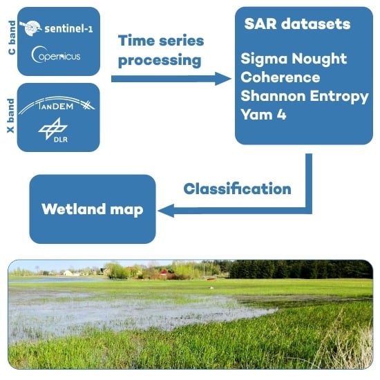
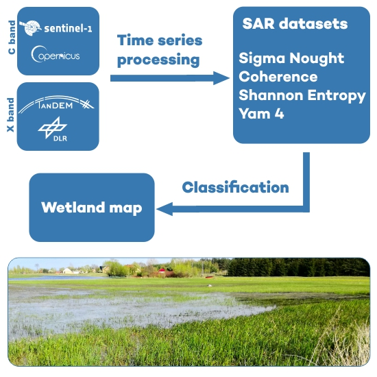
:This research is related to the eco-hydrological problems of the herbaceous wetland drying and biodiversity loss in the floodplain lakes of the Middle Basin of the Biebrza River (Poland). An experiment was set up, with its main goals as follows: (i) mapping the vegetation types and the temporarily or permanently flooded areas, and (ii) comparing the usefulness of the C-band Sentinel-1A (S1A) and X-band TerraSAR-X/TanDEM-X (TSX/TDX) for mapping purposes. The S1A imagery was acquired on a regular basis using the dual polarization VV/VH and the Interferometric Wide Swath Mode. The TSX/TDX data were acquired in quad-pol, a fully polarimetric mode, during the Science Phase. The paper addresses the following aspects: (i) wetland mapping with the S1A multi-temporal series; (ii) wetland mapping with the fully polarimetric TSX/TDX data; (iii) comparing the wetland mapping using dual polarization TSX/TDX subsets, that is, the HH-HV, HH-VV and VV-VH; (iv) comparing wetland mapping using the S1A and TSX/TDX data based on the same polarization (VV-VH); (v) studying the suitability of the Shannon Entropy for wetland mapping; and (vi) assessing the contribution of interferometric coherence for wetland classification. Though the experimental results show the main limitations of the S1A dataset, they also highlight the good accuracy that can be achieved using the TSX/TDX data, especially those taken in fully polarimetric mode. Some practical outcomes significant for the study area management using SAR were also described.
1. Introduction
As stated in Reference [1], the need for wetland mapping has never been greater as the world’s population continues to increase. The impact of climate change combined with the human activity that is transforming wetlands into meadows or pastures have led, in many geographical contexts, to wetlands degradation, drying of soils, and biodiversity loss. Nowadays, positive water balance and longer periods of water stagnation are crucial factors in the wetlands re-naturalization process and conservation.
The main motivation of this research is related to the eco-hydrological problems of the herbaceous wetland drying and biodiversity loss in the floodplain lakes of the Middle Basin of the Biebrza River (Poland). In this area, the problems of soil moisture and biomass estimation have been intensively studied in the past [2,3]. The main hydrological concern in this area is how to retain the water for longer periods from early spring flooding. The deficit of water is a factor influencing the life conditions of the ichthyofauna and avifauna. Further consequences of the water deficit are the unfavorable vegetation succession and the reduction of the quantity of species.
Eco-hydrological investigations of wetlands bring essential information for ecological inventory and wetland management. They need to be based on detailed mapping of the vegetation and the monitoring of changing water conditions. Wetland mapping using radar remote sensing has developed rapidly over the past years thanks to the wide availability of SAR imagery and the increased geometric resolution of SAR sensors. Wetlands have specific and advantageous features in relation to the microwave scattering mechanism. In fact, microwaves are sensitive to differences in water content and surface roughness. An increase of moisture or roughness results in an increase of the backscatter. In general, the results of SAR-based land cover and vegetation mapping depend on the used wavelength (the X, C, or L band) and data polarization (vertical, VV; horizontal, HH; or orthogonal, VH or HV). This is one of the issues examined in this work. It should also be noted that imaging angles and local incidence angles can also modify the power of the backscattered signal. In case of relatively flat wetland areas, the imaging angles were taken into account or at least analyzed in previous research; for example, Schlaffer et al. [4] and Marechal et al. [5]. In the work of Schlaffer et al., based on the Envisat ASAR Wide Swath images, a linear shift in average backscatter of wetland for three ranges of incidence angles (15–25, 25–35 and 35–45 degrees) was observed. The conclusion drawn was that “a good trade-off was obtained between robustness to surface roughness for open water classification and canopy attenuation for the classification of vegetated wetlands” [4] at intermediate incidence angles. The presence of water bodies or a water table with partially submerged plant communities creates the conditions for phase coherence preservation due to the double bounce effect. The coherence image can be one of the discriminators for land cover mapping, especially in context of wetlands [6,7], or can help in the estimation of water level for flood mapping [8]. It is worth mentioning that steep incidence angles can sometimes reinforce the double-bounce contribution in the case of submerged vegetation [4].
The launch of the ESA’s Sentinel-1A (S1A) satellite in 2014 opened a new chapter of SAR mapping. Free and open access was guaranteed to C-band SAR scenes in the dual polarization configuration VV-VH. Key advantages of the S1A included the observation of large swaths (250 km), the 12-day repetition cycle (using S1A or S1B only), the availability of two operational sensors and the access to SAR imagery at zero cost. The high temporal resolution of the Sentinel-1 images was exploited by Cazals et al. [9] for mapping and for the hydrological dynamics investigations of the coastal marshes. The researchers focused on three main classes only: open water, flooded vegetation, and non-flooded grasslands, using a supervised thresholding algorithm based on the hysteresis thresholding technique. Their results revealed the great potential of high frequency Sentinel-1 observations for hydrological regime identification and mapping. However, flooded grasslands with emergent vegetation were detected “with moderate accuracy” [9].
The availability of fully polarimetric SAR (HH/HV/VH/VV channels) could provide additional information on the structure and moisture of the vegetation, thus improving the utility of SAR data for wetland mapping [1,10,11]. However, the sources of fully polarimetric spaceborne SAR data are limited to the C-band Radarsat-2 and the L-band ALOS-PALSAR. In the work of Marechal et al. [5], the fully-polarimetric C-band Radarsat-2 time-series was evaluated for wetlands delineation and detailed vegetation mapping. The seasonal dynamics of the extent of the saturated areas in wetlands were also studied. Different polarimetric decomposition methods were investigated, and among them the Shannon Entropy (SE) “showed the most pronounced contrast between the marsh flooded areas and the surrounding areas” [5]. Based on this observation, we decided to include SE in our investigations using the X-band data. Another interesting conclusion issued from this research was that no significant differences in the delineation of water–saturated areas were observed for the images taken at different incidence angles. Niculescu et al. [12] describes the results of the experiment conducted on the Danube Delta floodable area with L-band ALOS/PALSAR data showing the usefulness of polarimetric entropy and temporal entropy to map changes of flood extent and land cover classes “characterized by more than one backscattering mechanism” [12]. In their approach, the HH and HV polarization channels were exploited.
In the X-band, interesting experimental campaigns based on the TSX/TDX satellites, forming a “fully polarimetric constellation”, were carried out by DLR—Deutsches Zentrum für Luft- und Raumfahrt in 2010 and 2014–2015 at a limited number of test sites around the globe. In addition to the evaluation of the potential of the S1A imagery, in this work, we decided to investigate the “fully polarimetric TSX/TDX constellation”. The Biebrza area was proposed to DLR as a test site during the Science Phase of the TSX/TDX mission. The main goals of this test site were: (i) mapping the vegetation types/associations/species and the temporarily or permanently flooded areas, and (ii) comparing the usefulness of S1A and TSX/TDX for mapping purposes. The main outcomes of this research are described in this paper.
To summarize, this work addresses the following main aspects:
- Mapping wetland with only the C-band S1A, based on the multi-temporal series of SAR images with coarser geometric resolution and fixed polarizations (VV-VH).
- Mapping wetland with experimental fully polarimetric quad-pol X-band TSX/TDX data with higher geometric resolution.
- Compare the wetland mapping using the dual polarization TSX/TDX subsets; that is, HH-HV, HH-VV, and VV-VH. These subsets represent the standard products that could be acquired by an operational X-band SAR sensor outside of special observation campaigns.
- Compare wetland mapping using S1A and TSX/TDX data based on the same polarization (VV-VH) and covering the same observation period—enhancing the differences in geometric resolution and its effect on classification accuracy.
- Study the suitability of the Shannon Entropy as a polarimetric descriptor of wetland land cover, starting from dual-pol and quad-pol data.
- Assess the contribution of interferometric coherence as an additional layer for land cover classification over wetland.
This paper is organized as follows: Section 2 describes the materials and methods. This includes the description of the study area and of the analyzed S1A and TSX/TDX datasets; the discussion of the image pre-processing carried out in this study; and the description of the image classification approach. Section 3 discusses the main results of this work. Finally, Section 4 includes the main conclusions of this study.
2. Materials and Methods
2.1. Description of the Study Area and the Available Ground Truth
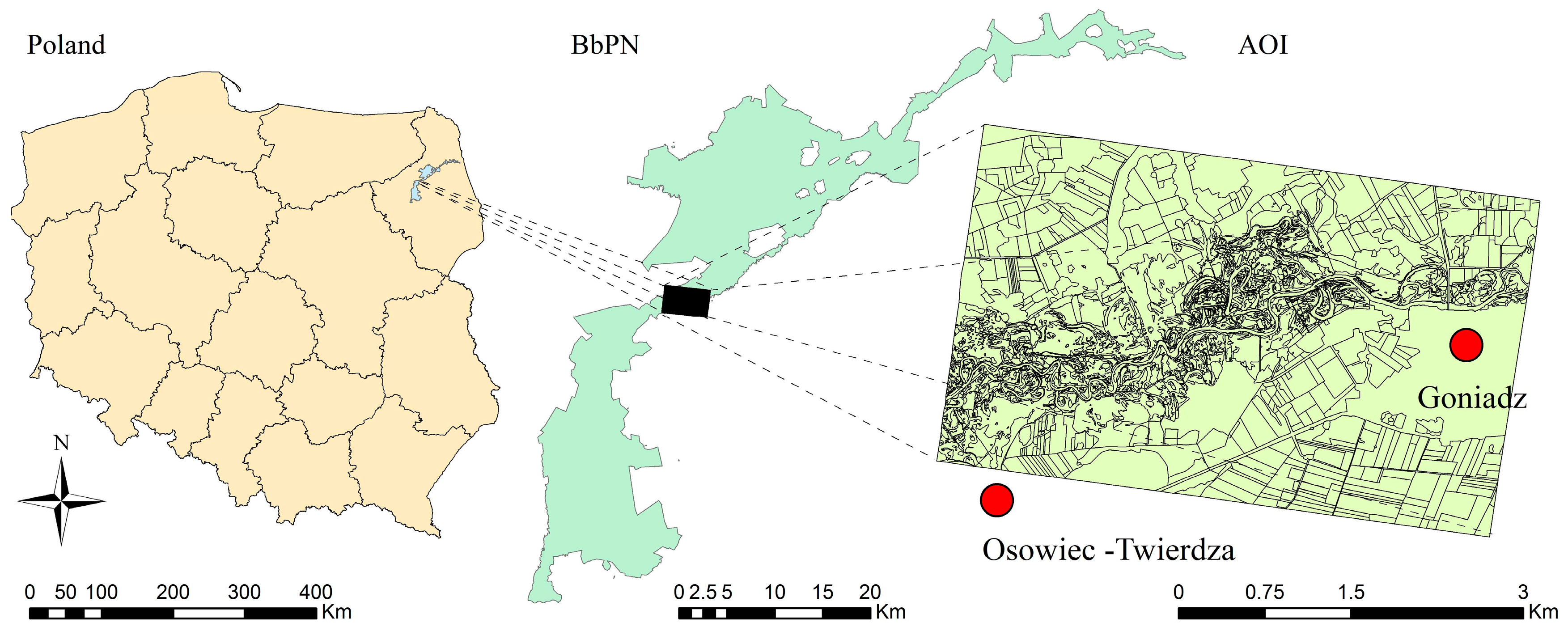
The Area of Interest (AoI) is part of the Middle Basin of the Biebrza Valley, in the Biebrza National Park (BbPN) [13], located in north eastern Poland (Figure 1). The Biebrza marshes represent an important wetland area, which is included in the United Nations Ramsar Convention on Wetlands [14]. The investigated area is mainly characterized by numerous meanders of the main stream and many oxbow lakes, with different degrees of hydrological connectivity. The study area was restricted to natural vegetation communities only, while the agricultural areas were excluded. The most dominating vegetation species are bur-reed, sweet-grass, reed canary, lakeshore bulrush, bulrush, common reed, sedge, dogwood, willow scrub, and deciduous forest. The most characteristic hydrological phenomenon in this area is the occurrence of an annual spring flooding which causes an increase in the biodiversity of the area. The snow melt is the most important source of water, but the period of water stagnation is relatively short due to the artificial drainage network built 50 years ago that enables fast water transfer from the Middle to the Lower Basin.
An important database of the vegetation and land cover of the study area was established using data from external Geographic information system (GIS) databases, land registers, and several field surveys made in correspondence to the radar image acquisition dates. The ground truth collection was made by botanists and hydrologists with the support of aerial imagery from several surveys using an Unmanned Aerial System (UAS) system equipped with a red-green-blue (RGB) camera. The photointerpretation of multi-temporal RGB images combined with in-situ GPS measurements allowed us to draw accurate polygons of the different thematic classes of the area.
Table 1 contains the information on the vegetation types considered in this study, and their statistical representation using the S1A and TSX/TDX data.
2.2. Sentinel-1A and TSX/TDX Datasets
In this study, two radar-image time-series were used: the S1A and the TSX/TDX. The main characteristics of the TSX/TDX and S1A data are shown in Table 2. The S1A imageries were acquired on a regular basis using the dual polarization VV/VH and the Interferometric Wide Swath Mode. The S1A dataset consists of Single Look Complex (SLC) images, acquired with a look-angle of 38.9 deg. at the centre of the AoI. The TSX/TDX data were acquired in the quad-pol, fully-polarimetric mode during the Science Phase of the missions. The main goal of the Science Phase was the demonstration of new SAR techniques. See Reference [15] for details. The Science Phase lasted 15 months, starting in October 2014 and ending in December 2015. Within this time two main operation modes were executed; the pursuit monostatic and the bistatic mode with varying perpendicular and along-track baselines.
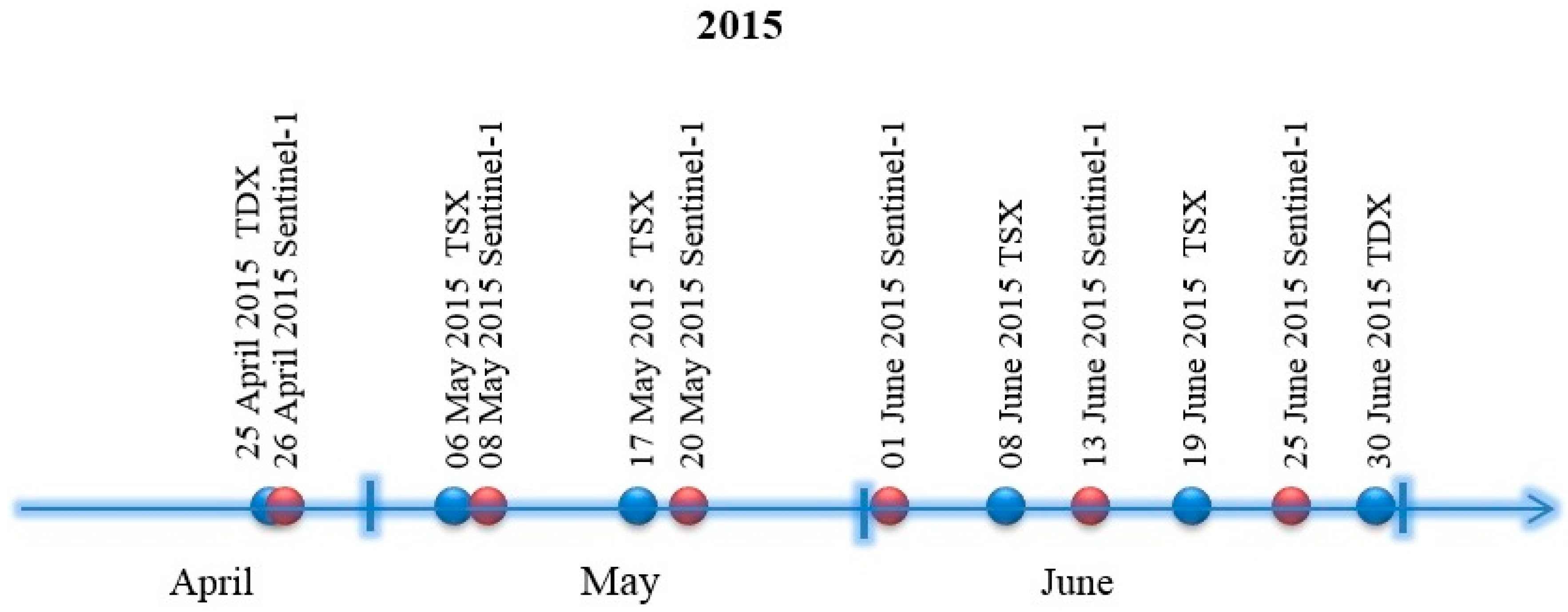
The bistatic phase started in March 2015 and was in use until the end of the Science Phase. The Dual Receive Antenna mode was available for both operation modes enabling the acquisition of fully polarimetric data. The used TSX/TDX images were Co-registered Single-look Slant-range Complex (CoSSC) products, acquired in the StripMap mode, with a look-angle of 36°—very close to the S1A look-angle. The data covered a two-month period (Figure 2), which included a spring flooding and the subsequent dynamic vegetation development of the wetlands.
2.3. Image Pre-Processing
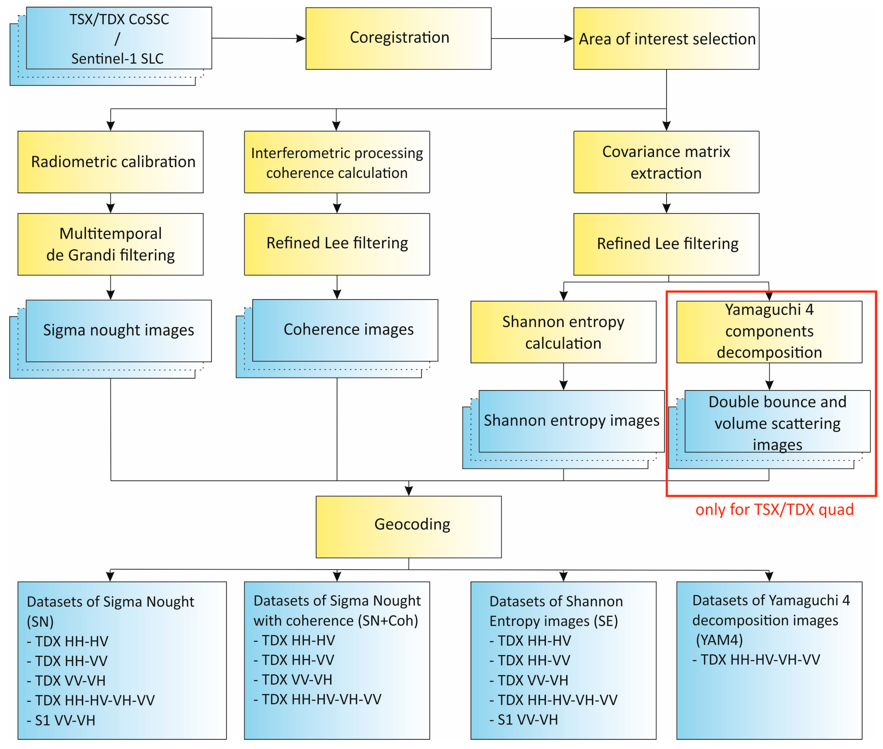
This work involved a set of image pre-processing steps. The workflow of the image pre-processing is shown in Figure 3.
The first step is image co-registration, which is followed by AoI selection. For both sensors, the radiometric calibration is performed using Equations (1) and (2) [16,17]:
where is the radar brightness, called Beta Nought; is the calibration coefficient; and and are the real and imaginary parts of the backscattered complex signal, respectively. The images are then converted into sigma nought images in the logarithmic scale (dB):
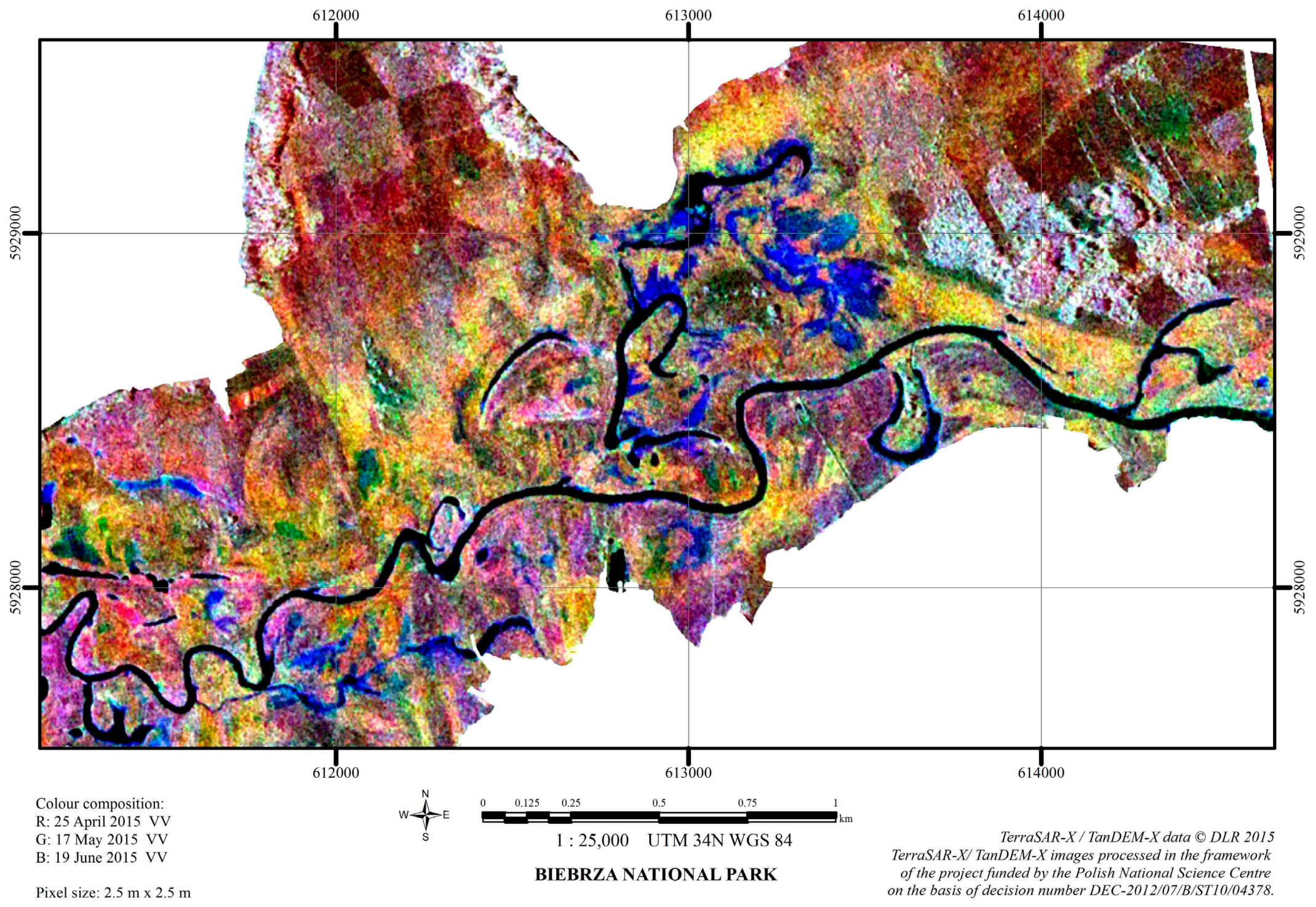
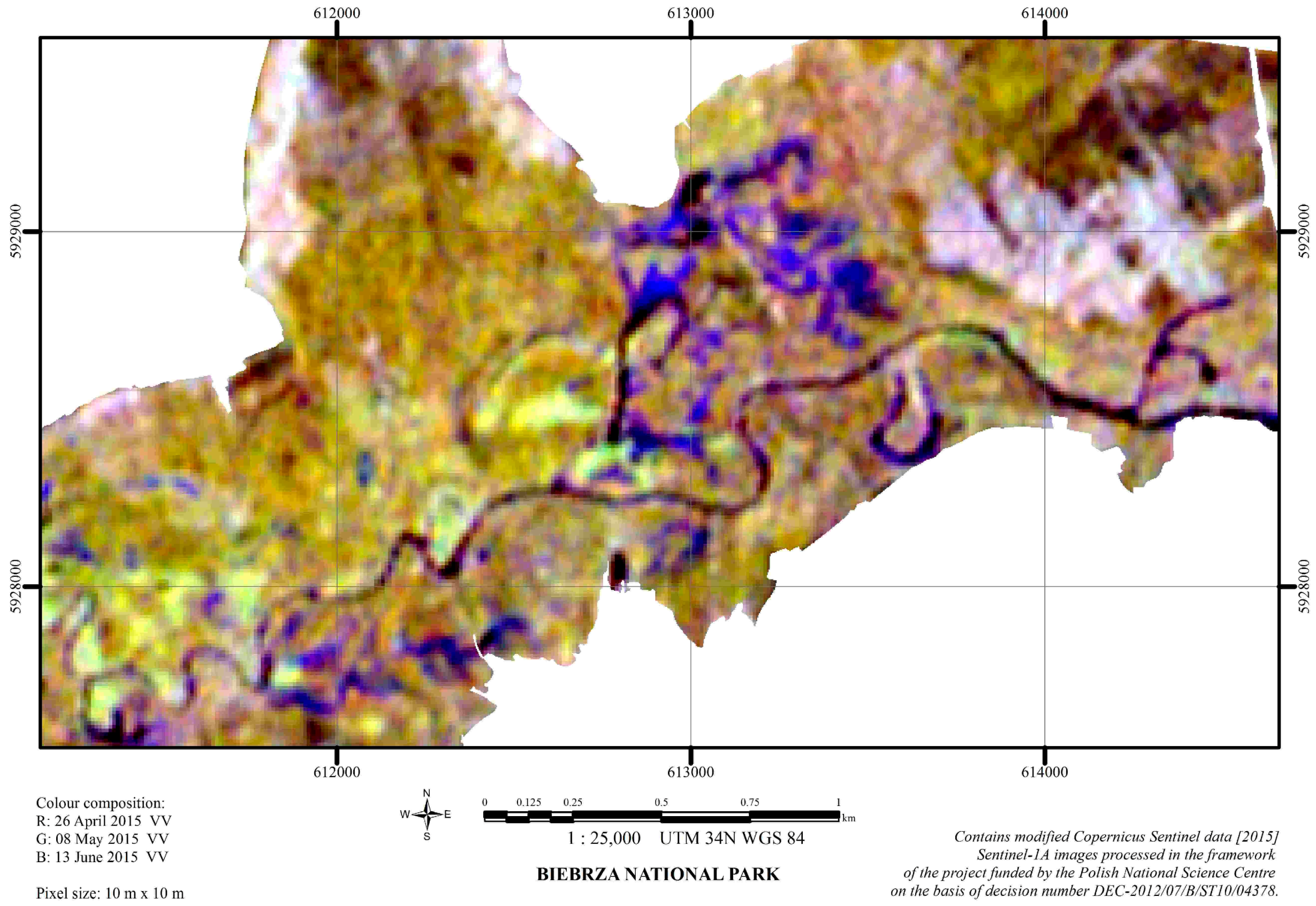
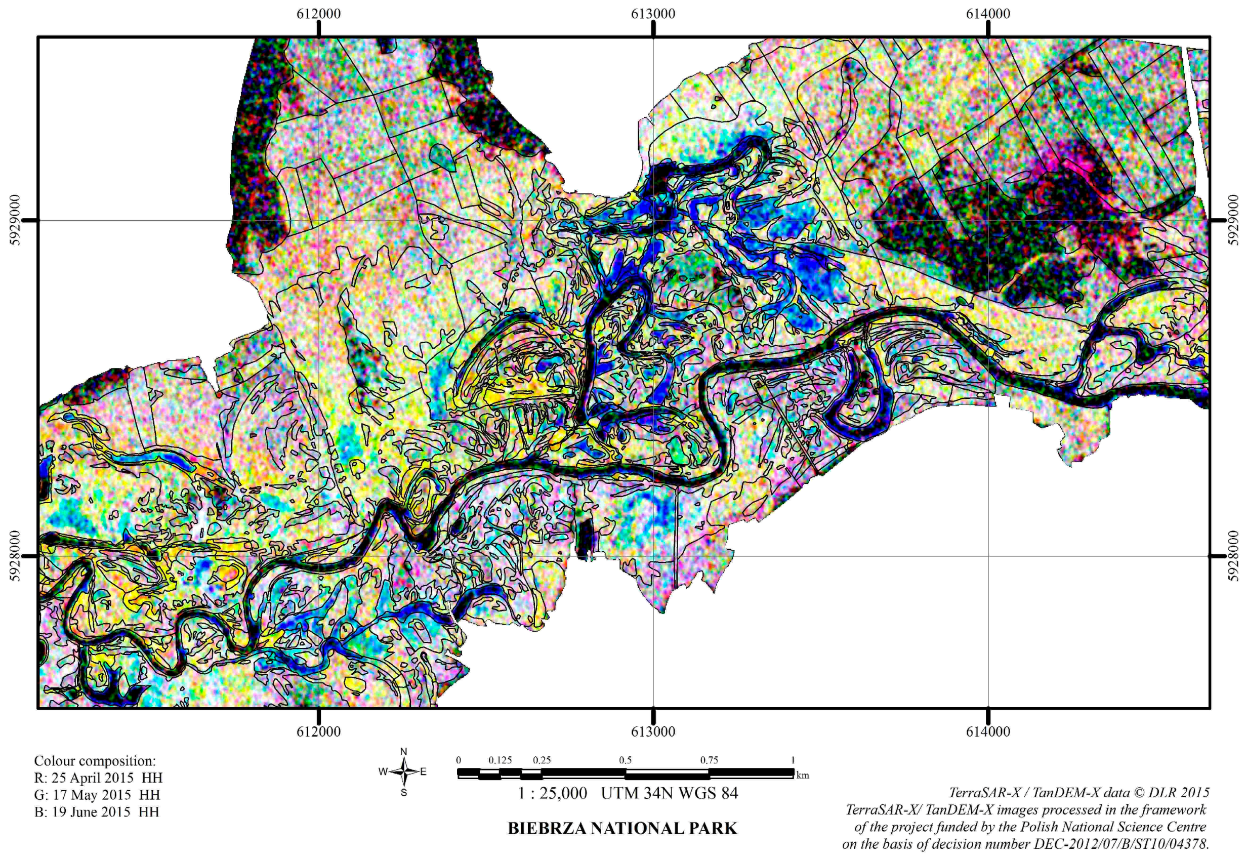
where θ is the radar incidence angle. Prior to the conversion from the linear scale to the decibel scale, the multi-temporal de Grandi filter [18] is applied, using a 3 × 3 window to reduce the speckle effect independently for each polarization channel for both image stacks. The calibrated and filtered images are then geocoded using a Digital Elevation Model (DEM) from the Shuttle Radar Topography Mission (SRTM) mission [19,20], forming the First Dataset “Sigma Nought” (SN). Examples of color compositions consisting of selected SN images are shown in Figure 4 and Figure 5. The difference in resolution was clearly visible between the TSX/TDX and S1A, as well as the contrast between land cover between the HH and VV polarizations.
The coherence is another parameter considered in this study. It is calculated between consecutive images with a temporal separation of 11 days (TSX/TDX) or 12 days (S1A), using this formula [21]:
where is the coherence (ranging from 0 to 1), and are the complex SAR images, is the expected value, and indicates the complex conjugate.
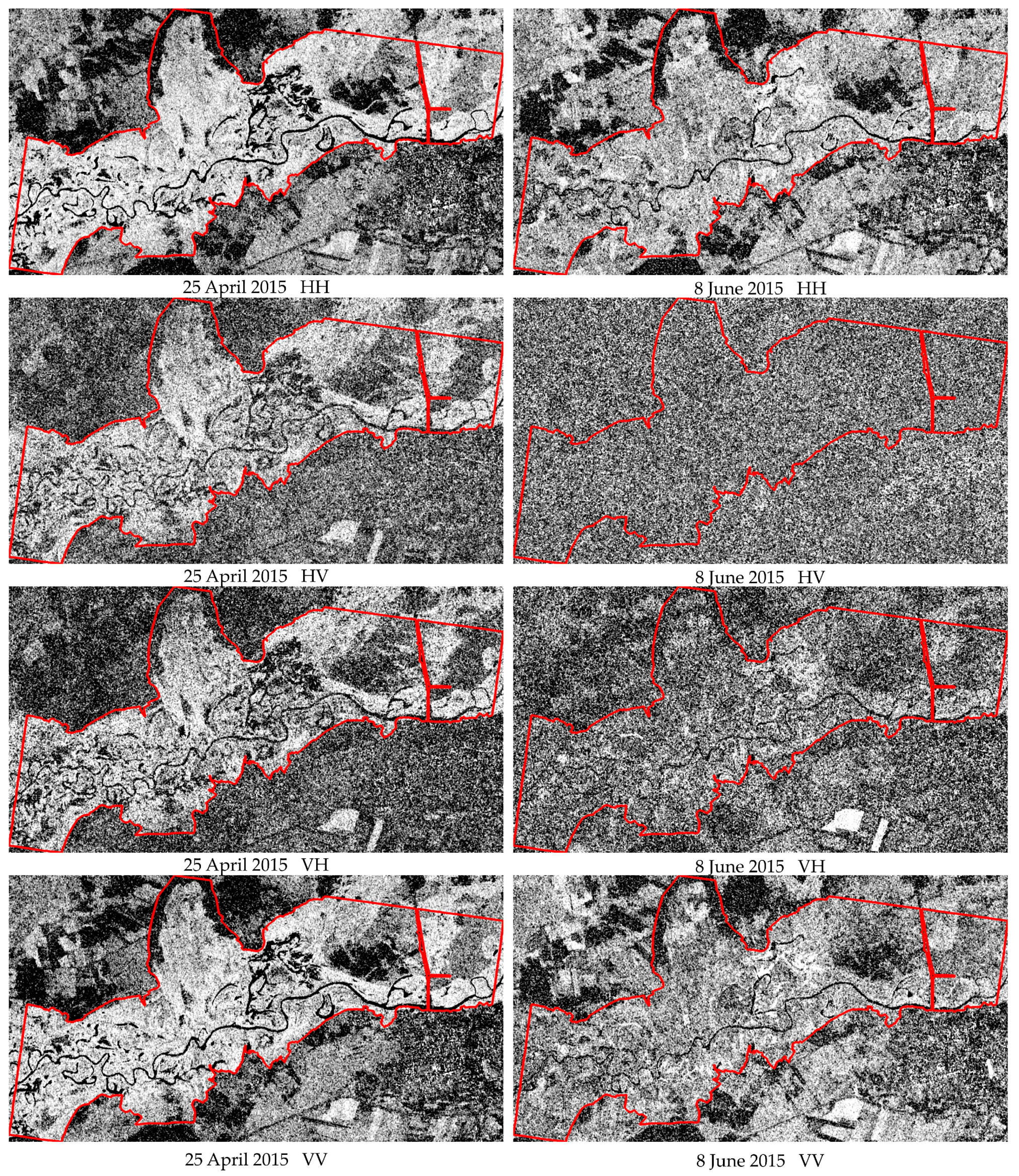
Over the vegetated areas, the 11-day and 12-day coherence images showed very low values and no contrast, hence demonstrating their uselessness for mapping purposes. On the other hand, it was possible to compute the coherence of TSX/TDX data acquired quasi-simultaneously in the monostatic or bistatic tandem modes (with a perpendicular baseline of 1.9 km and an across baseline of 300 m). In these coherence images, there are differences between different types of land cover, mostly between trees, open water, and semi-natural herbaceous vegetation; for examples, see Figure 6. The contrast between land cover types depends on the date of acquisition and polarization. The contribution of this information was analyzed in this study, considering a second dataset called “Sigma Nought + Coherence” (SN + coh). An example of the color composition using three coherence images corresponding to three different dates is shown in Figure 7. It can be observed that, for different parts of the image, the coherence changes over time.
The analysis of the polarimetric features of the considered data is another component of this study. This was done through polarimetric decompositions, which reveal the scattering mechanisms that are dependent on object structure, dimension, and moisture, and are classified in surface scattering, volume scattering, and double bounce. The Shannon Entropy (SE) can be extracted from quad-pol (TSX/TDX) and dual-pol data (S-1 and TSX/TDX). SE, which measures the randomness of the scattering of a pixel [22], was extracted from a co-variance matrix using the PolSARpro 5.0 software. SE is the sum of two contributions: intensity related (), which depends on total backscattered power, and polarimetry related (), which depends on the degree of polarization [23]. The SE is given by the following formulae [22,23]. For dual polarization data:
For fully polarimetric data (quad-pol):
where is the trace of matrix, is the covariance matrix, is the coherence matrix, are the intensities, and are the degrees of polarization.
High values of the component, which means a high degree of phase randomness, were observed over open water and dense vegetation (grass). High values of and low values of are associated with the double bounce effect over urban areas and some crops, like corn outside of the main AoI, as well as partially flooded vegetation and common reed in the AoI.
The polarimetric decomposition of the TSX/TDX quad-pol data was based on the Yamaguchi four-component decomposition, which has a direct physical interpretation. The general formula, which is described in References [23,24], is:
where is the co-variance matrix, are coefficients, and are the mean co-variance matrices for each scattering mechanism: surface, double bounce, volume, and helix, respectively.
The CoSSC TSX/TDX and the SLC S1A images were processed using PolSARPro 5.0 [25] and SARScape 5.0 [26,27]. Co-registration, radiometric calibration, test area selection, multi-temporal de Grandi filtering, and interferometric processing, including coherence calculation and geocoding, were done using SARScape. The Lee speckle filtering [28], SE, and the Yamaguchi four-component decomposition were performed using PolSARPro. The output from the pre-processing stage were four datasets, which are listed in Table 3.
2.4. Multi-Temporal Image Classification
“Per pixel” classification of the datasets shown in Table 3 was carried out to retrieve thematic classes. The classification workflow is shown in Figure 8. The first step was in defining good and representative samples for the thematic classes (ROIs—Regions of Interest) and calculating their statistical signatures: mean, variance, and standard deviations. The ROIs were identified using the ground truth data. The list of classes, the number of representing pixels, and their surface area are shown in Table 1. The quality of the samples (signatures) is expressed by the number of pixels, their surface, and the mutual “spectral” separability. In fact, the supervised classification approach assumes that the thematic classes are sufficiently different spectrally. For each pair of classes, the separability was calculated using the Jeffries-Matussita Distance [29]. Other separability measures, like the Transformed Divergence, the Bhattacharyya distance [30,31], or the Hellinger distance [32] could also be applied.
If the separability verification is positive, the ROIs can then be split into training and control parcels and submitted for classification. A Jeffries-Matussita Distance higher than 1.8 was chosen as the threshold for criterion fulfillment. Otherwise, the ROIs have to be merged following their spectral similarity and thematic significance. This can be a time-consuming process. In order to facilitate it, in this work, a hybrid approach which combines a supervised classification with an unsupervised clustering technique was adopted. The clusters automatically generated by the ISODATA algorithm [33], after their thematic aggregation based on ground truth, reveal the objects that are truly consistent in the spectral space. The unsupervised classification results make the redefinition of ROIs faster and more appropriate for further supervised classification. The steering parameters of clustering were carefully chosen because of the data heterogeneity. The following parameters were identified: minimum number of classes: 8; maximum number of classes: 12; maximum iterations: 30; change threshold: 1%; minimum number of pixels in class: 100; maximum standard deviation: 1; minimum class distance: 3; and maximum merge pairs: 2.
The supervised classification was performed using the Supported Vector Machine technique [22,34,35,36]. The advantage of this technique is that it does not require a large number of training samples [37], and the probability distribution is not assumed a priori [38]. The data were classified using the radial basis function kernel, with a penalty parameter of 100 and a high classification probability threshold of 0.9. The quality of classification was analyzed based on the classification accuracy, estimated by the User’s Accuracy, Producer’s Accuracy, Overall Accuracy (OAA) and the Kappa Index of Agreement (KIA) [39,40,41].
3. Results and Discussion
In order to correctly interpret the achieved results, we will reiterate the main goals of this work: (i) mapping the vegetation types/associations/species and the temporarily or permanently flooded areas, and (ii) comparing the performance of S1A and TSX/TDX for mapping purposes. The first goal embraces two interrelated phenomena: Vegetation and water regime. In wetlands, the types of vegetation (species and associations) develop and grow as a consequence of a multiannual water regime. The vegetation is then an indicator of preponderant moisture conditions, and the temporarily or permanently flooded areas allow the development of diversified hygrophilous associations. Considering these aspects while performing wetland classification provides useful information for eco-hydrological investigations and for wetland management.
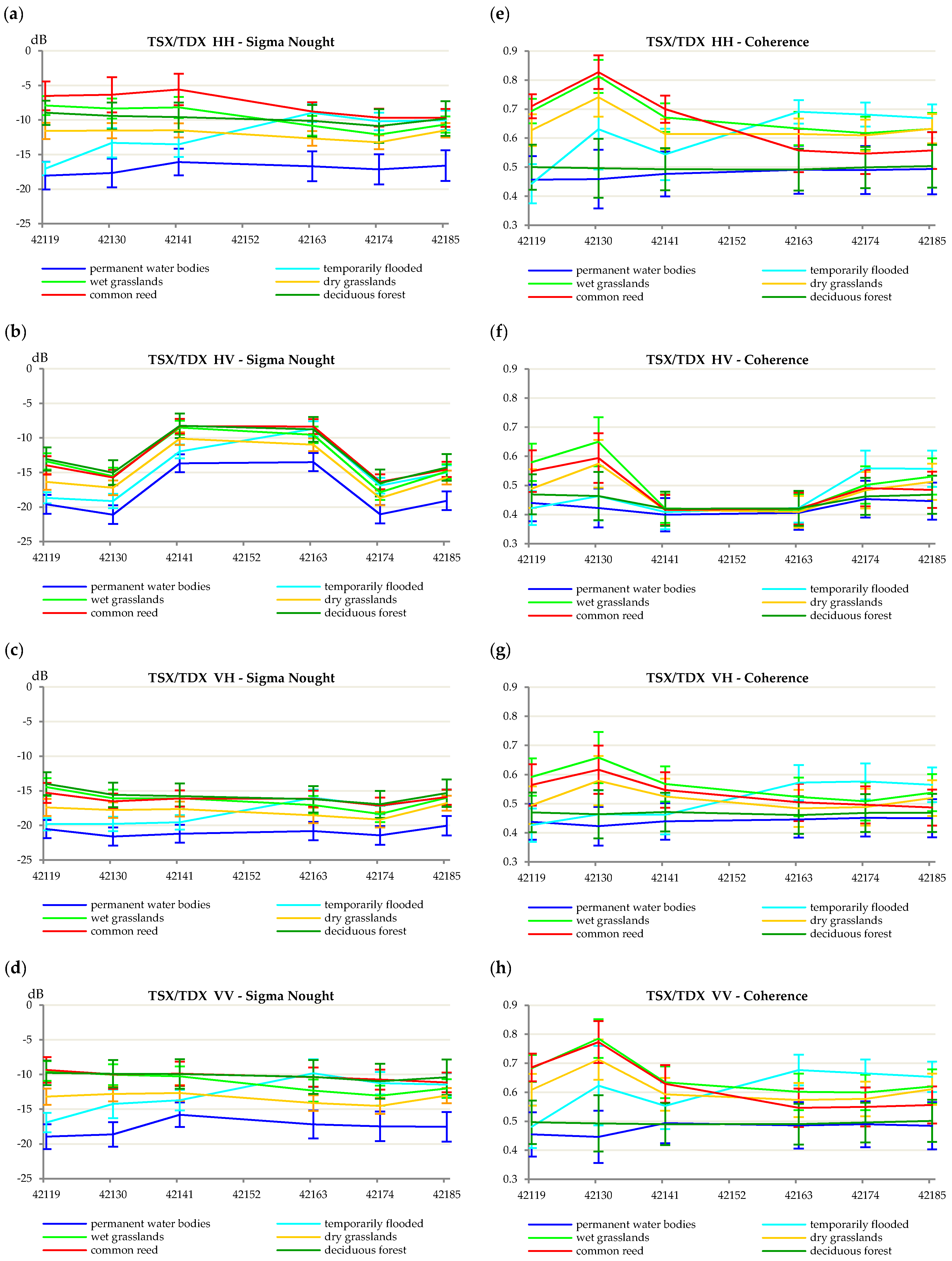
Referring to Table 1, some vegetation types (common reed, reed canary, sweet grass) possessed quite similar features regarding the microwave scattering mechanisms, for example, broad leaves and thin stems. For this reason, the set of thematic classes from Table 1 turned out to be too detailed to be distinguished by classification of the multi-temporal SAR images collected in this experiment. In fact, the classification based on initial samples only achieved a low accuracy level (OAA < 40%). It was then necessary to reduce the number of classes. For both the S1A and TSX/TDX datasets and an OAA exceeding of 40%, it was possible to distinguish six thematic categories: (1) permanent water bodies, (2) temporarily flooded areas, (3) wet grasslands, (4) dry grasslands, (5) common reed, and (6) deciduous forest. The number of classes, which is sensibly smaller than expected at the beginning of the experiment, was fixed for all datasets submitted for classification (see Table 4). For these six classes the temporal signatures representing sigma nought at different polarizations (see Figure 9a–d) and coherence values (mean and standard deviations) extracted from the TSX/TDX multi-temporal dataset are presented in the Figure 9e–h.
This example shows the discriminative subset and the coherence issued from the two simultaneous TSX/TDX acquisitions (zero temporal baseline). Some interesting features were observed from the graphs: (i) high temporal variability of sigma nought for the class of temporarily flooded areas occurring together with temporal variability of the coherence, (ii) there were quite significant differences of coherence values for some acquisitions and classes, confirming their potential as a class discriminator, (iii) unusual behavior of sigma nought (very high values) and the coherence (very low values) for two acquisitions at HV polarization (8 June 2015 and 17 June 2015). This last observation is confirmed in Figure 6 (right column). The explanation for this anomaly was not evident: neither instrument malfunctioning problems nor spectacular acquisition problems were reported.
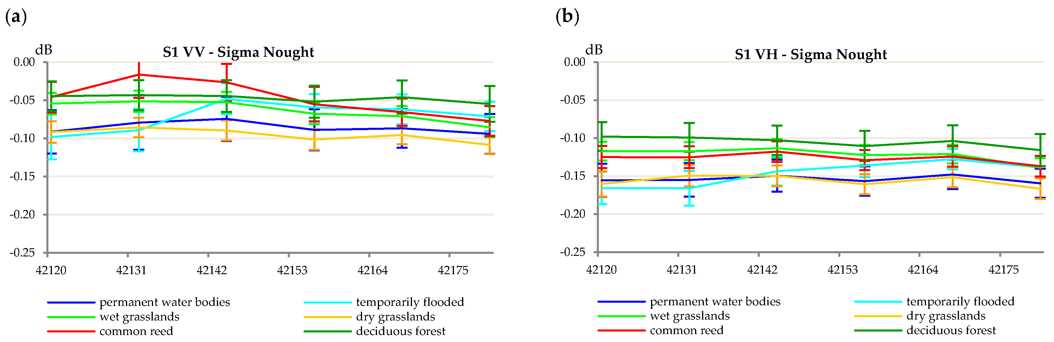
In Figure 10, one can observe the temporal profile of sigma nought for the final classes extracted from the Sentinel-1 time series. The profiles were quite similar except for the partially flooded areas at VV and VH polarization and for the common reed class at VV polarization. This similarity was further confirmed by the low values of OAA for the S1 time series.
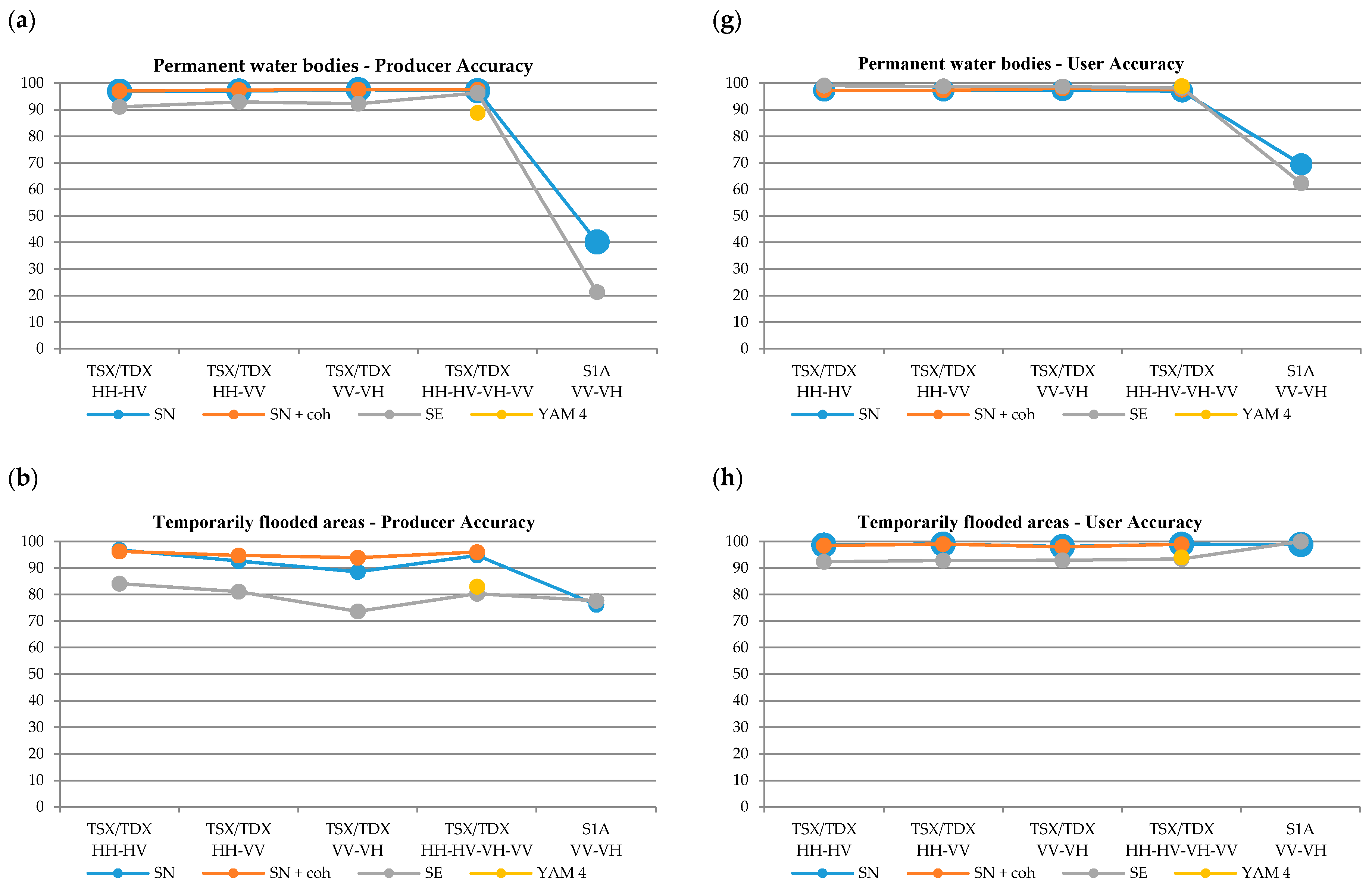
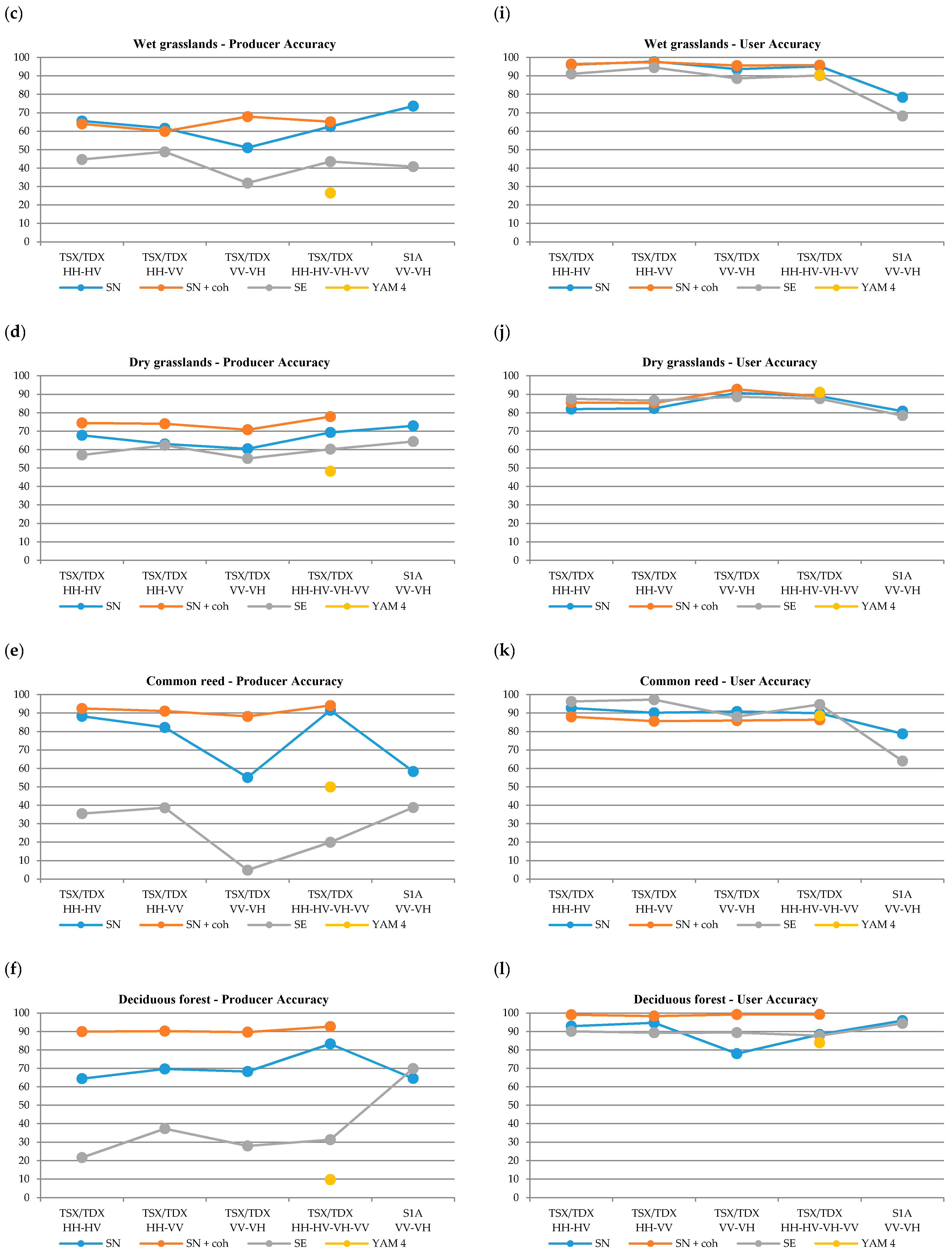
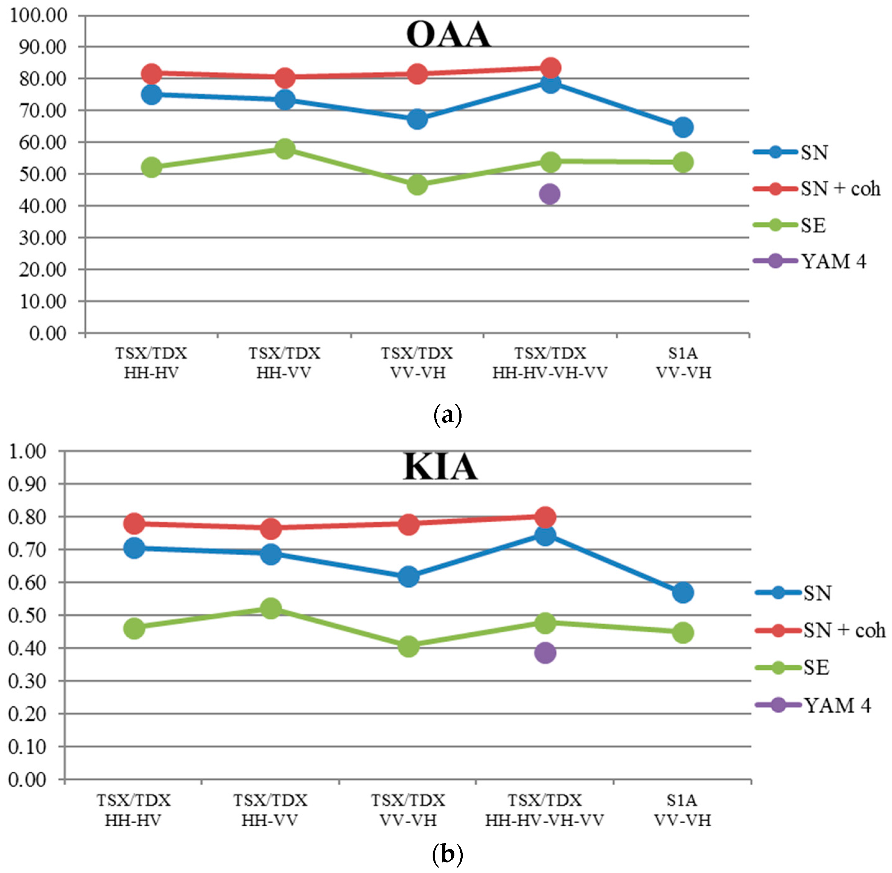
The results of the classification accuracy are presented in Figure 11 and Figure 12. In Figure 11 high differences of Producers’ Accuracy (Figure 11a–f) for all classes and data subsets except for the permanent water bodies could be observed. On the other hand, the Users’ Accuracies (Figure 11g–l) were generally close to each other for all classes and data subsets compared to the Producers’ Accuracy. Generally, Users’ Accuracies were higher than Producers’ Accuracies. As suggested in the literature, “it is critical that they both be considered when assessing the accuracy of the classified image/map” [40] for particular classes and cases. In the context of this work, in order to compare the accuracy for the six classes (Table 4) achieved with four types of data (Table 3), we compared the overall accuracies (OAA) as more synthetic measures of wetland map quality.
The results of the work can be summarized as follows, relating them to the aspects addressed in the introduction:
- Mapping wetlands with the C-band S1A alone, based on the multi-temporal series of SAR images with VV/VH polarization. The results achieved with the time series of S1A SN were quite poor. The OAA for all classes equaled 65% and the KIA was 0.58. These values were not satisfactory. For this reason, the S1A dataset was not recommended for herbaceous wetland mapping in the Biebrza valley. There was a second disadvantageous feature of the S1A dataset; its geometric resolution was too coarse to detect not only the small areas of vegetation associations adjacent to oxbows and floodplain lakes, but also the small permanent water bodies.
- Mapping wetlands with the experimental fully-polarimetric quad-pol X-band TSX/TDX data. The results achieved (polarizations VV/VH/HV/HH) are the best amongst all the SN time series. The OAA was 79%, with a high coefficient of agreement, KIA, of 0.75. The results achieved using the fully polarimetric data and the Yamaguchi four-component decomposition (YAM4) were less useful than expected because the OAA was 43% and the KIA was 0.39. For this area and for the majority of classes over time, the dominant scattering mechanism was volume scattering, which decreased the OAA. The advantage of this decomposition was in revealing partially flooded herbaceous vegetation by the double bounce effect for particular TSX/TDX acquisitions. The results achieved using SE decomposition were better than those using the YAM4 dataset: the OAA was 55% and the KIA was 0.48. This could have been caused by the intensity component contribution outside of the polarimetric behavior.
- Comparing wetland mapping using the dual polarization TSX/TDX subsets; that is, HH-HV, HH-VV and VV-VH. For the dual-pol TSX/TDX products, the OAA and KIA were smaller than those from the four polarizations dataset: OAA = 76% and KIA = 0.71 for HH/HV; OAA = 74% and KIA = 0.69 for HH/VV; and OAA = 68% and KIA = 0.63 for VV/VH. However, there was a relatively small difference between the results achieved by quad-pol and the best dual-pol (HH/HV). Thus, this configuration can be recommended for wetland mapping purposes.
- Comparing wetland mapping using S1A and TSX/TDX, considering the same polarization (VV-VH) and covering the same observation period. The TSX/TDX dataset showed better performance. The difference of the OAA for the S1A and TSX/TDX datasets was about 3%. It seemed that the coarser geometric resolution had a negative influence on the results achieved by the S1A dataset.
- Studying the suitability of the Shannon Entropy as polarimetric descriptor of wetland land cover. The results achieved with the SE time series were quite poor, with the OAA ranging from 47% to 58%, and KIA ranging from 0.41 and 0.52. As a consequence, this dataset is not recommended for the mapping of the herbaceous wetland at all. The OAA values are lower for the pairs of bands containing cross-pol components (VH or HV). According to Reference [22], these components are strongly affected by the noise equivalent sigma zero over wetlands areas, thus affecting the SE parameter.
- Assessing the contribution of the interferometric coherence as an additional layer for land cover classification. The interferometric coherence estimated for the acquisitions of S1A, with a 12-day interval, and TSX/TDX, with an 11-day interval, turned out to be useless as land cover discriminators over this wetland. On the other hand, the coherence calculated for the TSX/TDX interferometric pairs acquired simultaneously (at the same time from two sensors) causes an increase of the OAA comparing to the SN time series. The OAA increased 7% for the HH-HV and HH-VV, 15% for the VV-VH, and 4% for the VV-VH-HV-HH datasets. The interferometric coherence is considered an important asset of quad-pol TSX/TDX acquisitions.
Figure 13 shows a classification result over the AoI obtained using SN and the coherence time series of TSX/TDX data (four polarizations). This configuration achieved the best classification accuracy (OAA = 83%, KIA = 0.80).
4. Conclusions
In this comparative study, the use of the S1A and TSX/TDX image time series for herbaceous wetland mapping has been evaluated. The main components of the methodology used to carry out this work have been presented. Different aspects of data processing and analysis have been described. The main outcomes of the study are briefly summarized below.
Using image classification, in the AoI only, the main land cover types could be distinguished. In fact, exceeding an OAA of 40% for both the S1A and TSX/TDX datasets, it was possible to distinguish six thematic categories: (1) permanent water bodies, (2) temporarily flooded areas, (3) wet grasslands, (4) dry grasslands, (5) common reed, and (6) deciduous forest. In terms of vegetation mapping, the majority of species identified in-situ (listed in Table 1) had to be merged into two main categories: wet grassland habitat and dry grassland habitat. Concerning water stagnation mapping, it was possible to classify permanent water bodies and temporarily flooded areas. This second category includes the partially flooded grasslands that could be identified and mapped through the Shannon Entropy decomposition by exploiting the double bounce effect.
At the beginning of the project, the S1A imageries were identified as the primary dataset for thematic mapping. However, the S1A results achieved in this study show an important limitation of this type of data for the purpose of detailed wetland mapping. Advantages of S1A include its large area coverage and the possibility to extract information on partially flooded grasslands for the whole Biebrza valley area using the SE.
The results achieved using the time series of the TSX/TDX images, especially those taken in fully-polarimetric mode, show that the wetland mapping of the above-mentioned classes can be performed with satisfying accuracy, better than those achieved using the S1A imageries. The use of the four polarizations in the dataset shows the best accuracy using sigma nought values only. In addition, the use of the interferometric coherence, extracted from the TSX/TDX images acquired simultaneously, slightly increases this accuracy (2.5%).
The comparison of the results from the different dual polarizations (HH-HV, HH-VV, and VV-VH) versus the four polarizations leads to the conclusion that standard TSX/TDX Strip Map products acquired at HH-HV polarization provide the best data for wetland mapping. Similar to S1A, the partially flooded vegetation can be properly extracted using SE in this case as well. Furthermore, there is the additional advantage of a higher geometric resolution with respect to the S1A dataset. The results achieved in this work lead to the conclusion that the TSX/TDX sensors are well-suited to the needs of wetland mapping in terms of water time stagnation and its ecological implications, especially for fine oxbows and small floodplain lakes. The outcomes from the project were presented to the Biebrza National Park (BbNP) authorities. They see the possibilities of applying some results of the project in the BbNP’s Programme of Protective Tasks for:
- Open water mapping (flood) at the scale of the Middle and Lower Basins of the Biebrza River based on the dual-pol sigma nought time series of Sentinel-1 for assessing annual hydrological conditions influencing biodiversity.
- Submerged vegetation mapping both from the Sentinel-1 and the TerraSAR-X Strip Map for: (i) assessing annual hydrological conditions, and (ii) mapping the presence of water in the periods of grass mowing on the parcels used temporarily by farmers for hay production.
- Checking the common reed mowing during winter as agreed between BbNP and the farmers using the TerraSAR-X HH/HV dual-pol. This action is ecologically important for the improvement of the life conditions of wading birds.
Acknowledgments
This publication was prepared in the frame of the MARSHALL project, funded by the Polish National Science Centre (DEC-2012/07/B/ST10/04378). The authors acknowledge the German Space Agency DLR for providing the TerraSAR-X/TanDEM-X Quad-Pol images in the frame of the NTI_POLI 6756 “Oxbow Plus” project. This work contains modified Copernicus Sentinel data.
Author Contributions
Marek Mróz contributed to the design of the study and supervised the research. Magdalena Mleczko contributed to the methodology, performed image pre-processing, classifications and statistical analyses. Both authors collectively wrote the paper.
Conflicts of Interest
The authors declare no conflict of interest.
References
- Brisco, B. Mapping and Monitoring Surface Water and Wetlands with Synthetic Aperture Radar. In Remote Sensing of Wetlands: Applications and Advances; CRC Press: New York, NY, USA, 2015; pp. 119–136. ISBN 1482237385. [Google Scholar]
- Dabrowska-Zielinska, K.; Budzynska, M.; Tomaszewska, M.; Bartold, M.; Gatkowska, M.; Malek, I.; Turlej, K.; Napiorkowska, M. Monitoring wetlands ecosystems using ALOS PALSAR (L-Band, HV) supplemented by optical data: A case study of Biebrza Wetlands in Northeast Poland. Remote Sens. 2014, 6, 1605–1633. [Google Scholar] [CrossRef]
- Dabrowska-Zielinska, K.; Budzynska, M.; Tomaszewska, M.; Bartold, M.; Gatkowska, M. The study of multifrequency microwave satellite images for vegetation biomass and humidity of the area under Ramsar convention. In Proceedings of the 2015 IEEE International Geoscience and Remote Sensing Symposium (IGARSS), Milan, Italy, 26–31 July 2015; Volume 2015, pp. 5198–5200. [Google Scholar]
- Schlaffer, S.; Chini, M.; Dettmering, D.; Wagner, W. Mapping wetlands in Zambia using seasonal backscatter signatures derived from ENVISAT ASAR time series. Remote Sens. 2016, 8, 402. [Google Scholar] [CrossRef]
- Marechal, C.; Pottier, E.; Hubert-Moy, L.; Rapinel, S. One year wetland survey investigations from quad-pol RADARSAT-2 time-series SAR images. Can. J. Remote Sens. 2012, 38, 240–252. [Google Scholar] [CrossRef]
- Hong, S.H.; Wdowinski, S. Double-bounce component in cross-polarimetric SAR from a new scattering target decomposition. IEEE Trans. Geosci. Remote Sens. 2014, 52, 3039–3051. [Google Scholar] [CrossRef]
- Kim, S.; Wdowinski, S.; Amelung, F.; Dixon, T.H.; Won, J.-S. Interferometric Coherence Analysis of the EvergladesWetlands, South Florida. IEEE Trans. Geosci. Remote Sens. 2013, 51, 5210–5224. [Google Scholar] [CrossRef]
- Pulvirenti, L.; Chini, M.; Pierdicca, N.; Boni, G. Use of SAR data for detecting floodwater in urban and agricultural areas: The role of the interferometric coherence. IEEE Trans. Geosci. Remote Sens. 2016, 54, 1532–1544. [Google Scholar] [CrossRef]
- Cazals, C.; Rapinel, S.; Frison, P.-L.; Bonis, A.; Mercier, G.; Mallet, C.; Corgne, S.; Rudant, J.-P. Mapping and Characterization of Hydrological Dynamics in a Coastal Marsh Using High Temporal Resolution Sentinel-1A Images. Remote Sens. 2016, 8, 570. [Google Scholar] [CrossRef]
- Touzi, R. Target scattering decomposition in terms of roll-invariant target parameters. IEEE Trans. Geosci. Remote Sens. 2007, 45, 73–84. [Google Scholar] [CrossRef]
- Baghdadi, N.; Bernier, M.; Gauthier, R.; Neeson, I. Evaluation of C-band SAR data for wetlands mapping. Int. J. Remote Sens. 2001, 22, 71–88. [Google Scholar] [CrossRef]
- Niculescu, S.; Lardeux, C.; Hanganu, J.; Mercier, G.; David, L. Change detection in floodable areas of the Danube delta using radar images. Nat. Hazards 2015, 78, 1899–1916. [Google Scholar] [CrossRef] [Green Version]
- Biebrza National Park. Available online: https://www.biebrza.org.pl/lang,2 (accessed on 31 October 2017).
- Ramsar the List of Wetlands of International Importance. Ramsar 2016, 1–48. Available online: http://www.ramsar.org/pdf/sitelist.pdf (accessed on 31 October 2017).
- Hajnsek, I.; Busche, T.; Krieger, G.; Zink, M.; Schulze, D.; Moreira, A. Tandem-X Ground Segment, Announcement of Opportunity: Tandem-X Science Phase; Microwaves and Radar Institute of the German Aerospace Centre (DLR): Oberpfaffenhofen, Germany, 2014; pp. 1–27. [Google Scholar]
- Nuno, M.; Meadows, P.J. Radiometric Calibration of S-1 Level-1 Products Generated by the S-1 IPF; Tech. Note; European Space Agency: Paris, France, 2015; pp. 1–13. [Google Scholar]
- Infoterra an EADS Astrium Company. Radiometric Calibration of TerraSAR-X Data, Beta Naught and Sigma Naught Coefficient Calculation; Infoterra an EADS Astrium Company: Friedrichshafen, Germany, 2008; pp. 1–16. [Google Scholar]
- De Grandi, G.F.; Leysen, M.; Lee, J.S.; Schuler, D. Radar reflectivity estimation using multiple SAR scenes of the same target: Technique and applications. In Proceedings of the International Geoscience and Remote Sensing Symposium (IGARSS), Singapore, 3–8 August 1997; Volume 2, pp. 1047–1050. [Google Scholar]
- Rosen, P.A.; Hensley, S.; Gurrola, E.; Rogez, F.; Chan, S.; Martin, J.; Rodriguez, E. SRTM C-band topographic data: Quality assessments and calibration activities. In Proceedings of the IEEE 2001 International Geoscience and Remote Sensing Symposium (Cat. No.01CH37217), Sydney, NSW, Australia, 9–13 July 2001; Volume 2, pp. 739–741. [Google Scholar]
- Marschalk, U.; Roth, A.; Eineder, M.; Suchandt, S. Comparison of DEMs derived from SRTM/X- and C-band. In Proceedings of the 2004 IEEE International Geoscience and Remote Sensing Symposium (IGARSS’04), Anchorage, AK, USA, 20–24 September 2004; Volume 7, pp. 4531–4534. [Google Scholar]
- Hanssen, R.F. Radar Interferometry—Data Interpretation and Error Analysis; Springer: Dordrecht, The Netherlands, 2001; Volume 2, ISBN 978-0-7923-6945-5. [Google Scholar]
- Betbeder, J.; Rapinel, S.; Corgne, S.; Pottier, E.; Hubert-Moy, L. TerraSAR-X dual-pol time-series for mapping of wetland vegetation. ISPRS J. Photogramm. Remote Sens. 2015, 107, 90–98. [Google Scholar] [CrossRef] [Green Version]
- Lee, J.-S.; Pottier, E. Polarimetric Radar Imaging: From Basics to Applications; CRC Press: Boca Raton, FL, USA, 2009; Volume 440. [Google Scholar]
- Cloude, S. Polarisation: Applications in Remote Sensing; Oxford University Press: Oxford, UK, 2009; ISBN 9780199569731. [Google Scholar]
- Pottier, E.; Ferro-Famil, L. PolSARPro V5.0: An ESA educational toolbox used for self-education in the field of POLSAR and POL-INSAR data analysis. In Proceedings of the International Geoscience and Remote Sensing Symposium (IGARSS), Munich, Germany, 22–27 July 2012; pp. 7377–7380. [Google Scholar]
- Sarmap. Available online: http://www.sarmap.ch/ (accessed on 31 October 2017).
- Simonetto, E.; Follin, J.M. An overview on interferometric SAR software and a comparison between DORIS and SARSCAPE Packages. In Geospatial Free and Open Source Software in the 21st Century; Lecture Notes in Geoinformation and Cartography; Springer: Berlin/Heidelberg, Germany, 2012; pp. 107–122. [Google Scholar]
- Lee, J. Sen Speckle analysis and smoothing of synthetic aperture radar images. Comput. Graph. Image Process. 1981, 17, 24–32. [Google Scholar] [CrossRef]
- Richards, J.A. Remote Sensing with Imaging Radar; Springer: Berlin/Heidelberg, Germany, 2009; ISBN 9783642020193. [Google Scholar]
- Morio, J.; Refregier, P.; Goudail, F.; Dubois-Fernandez, P.C.; Dupuis, X. A characterization of shannon entropy and bhattacharyya measure of contrast in polarimetric and interferometric SAR image. Proc. IEEE 2009, 97, 1097–1108. [Google Scholar] [CrossRef]
- Chung, J.K.; Kannappan, P.L.; Ng, C.T.; Sahoo, P.K. Measures of distance between probability distributions. J. Math. Anal. Appl. 1989, 138, 280–292. [Google Scholar] [CrossRef]
- Lee, K.Y.; Bretschneider, T.R. Separability measures of target classes for polarimetric synthetic aperture radar imagery. Asian J. Geoinform. 2012, 12, 27–46. [Google Scholar]
- Tou, J.T.; Gonzalez, R.C. Pattern Recognition Principles; Addison-Wesley Publishing Company: Reading, MA, USA, 1974; pp. 89–126. ISBN 9780201075861. [Google Scholar]
- Lardeux, C.; Frison, P.L.; Rudant, J.P.; Souyris, J.C.; Tison, C.; Stoll, B. Classification of fully polarimetric SAR data for land use cartography. ISPRS J. Photogramm. Remote Sens. 2006, 23–27. [Google Scholar] [CrossRef]
- Shah Hosseini, R.; Entezari, I.; Homayouni, S.; Motagh, M.; Mansouri, B. Classification of polarimetric SAR images using Support Vector Machines. Can. J. Remote Sens. 2011, 37, 220–233. [Google Scholar] [CrossRef]
- Sukawattanavijit, C.; Chen, J.; Zhang, H. GA-SVM Algorithm for Improving Land-Cover Classification Using SAR and Optical Remote Sensing Data. IEEE Geosci. Remote Sens. Lett. 2017, 14, 284–288. [Google Scholar] [CrossRef]
- Mantero, P.; Moser, G.; Serpico, S.B. Partially supervised classification of remote sensing images through SVM-based probability density estimation. IEEE Trans. Geosci. Remote Sens. 2005, 43, 559–570. [Google Scholar] [CrossRef]
- Ozdogan, M. Image classification methods in land cover and land use. In Remotely Sensed Data Characterization, Classification, and Accuracies; Prasad, S., Thenkabail, P.D., Eds.; CRC Press: Boca Raton, FL, USA, 2015; 712p, ISBN 978-1482217865. [Google Scholar]
- Hudson, W.D.; Ramm, C.W. Correct formulation of the Kappa coefficient of agreement. Photogramm. Eng. Remote Sens. 1987, 53, 421–422. [Google Scholar]
- Story, M.; Congalton, R.G. Accuracy assessment: A user’s perspective. Photogramm. Eng. Remote Sens. 1986, 52, 397–399. [Google Scholar] [CrossRef]
- Aronoff, S. Classification accuracy: A user approach. Photogramm. Eng. Remote Sens. 1982, 48, 1299–1307. [Google Scholar]
Figure 1.
Location of the study area in Northeastern Poland.

Figure 2.
Satellite images used in the study.

Figure 3.
The workflow of image pre-processing.

Figure 4.
The RGB color composition of “Sigma Nought” (SN) TSX images, with HH polarization, taken on the25 April 2015, 17 May 2015 and 19 June 2015 respectively.
Figure 4.
The RGB color composition of “Sigma Nought” (SN) TSX images, with HH polarization, taken on the25 April 2015, 17 May 2015 and 19 June 2015 respectively.

Figure 5.
The red-green-blue (RGB) color composition of SN S1A images, with VV polarization, taken on the 26 April 2015, 20 May 2015 and 13 June 2015 respectively.
Figure 5.
The red-green-blue (RGB) color composition of SN S1A images, with VV polarization, taken on the 26 April 2015, 20 May 2015 and 13 June 2015 respectively.

Figure 6.
Examples of the TSX/TDX coherence images for two different acquisition dates and four polarizations.
Figure 6.
Examples of the TSX/TDX coherence images for two different acquisition dates and four polarizations.

Figure 7.
The RGB color composition of the coherence change based on TSX/TDX images acquired at HH polarization, taken on the 25 April 2015, 17 May 2015 and 19 June 2015 respectively.
Figure 7.
The RGB color composition of the coherence change based on TSX/TDX images acquired at HH polarization, taken on the 25 April 2015, 17 May 2015 and 19 June 2015 respectively.

Figure 8.
The workflow of the thematic processing of the data subsets.

Figure 9.
Sigma nought (dB) (a–d) and coherence values (mean and standard deviations) (e–h) for the time series of TSX/TDX polarimetric acquisitions for the final six thematic classes.
Figure 9.
Sigma nought (dB) (a–d) and coherence values (mean and standard deviations) (e–h) for the time series of TSX/TDX polarimetric acquisitions for the final six thematic classes.

Figure 10.
Sigma nought (dB) (a) at VV and (b) VH polarizations (mean and standard deviations) for the time series of Sentinel-1A acquisitions for the final six thematic classes.
Figure 10.
Sigma nought (dB) (a) at VV and (b) VH polarizations (mean and standard deviations) for the time series of Sentinel-1A acquisitions for the final six thematic classes.

Figure 11.
The Producer’s (a–f) and User’s Accuracy (g–l) extracted from the confusion matrices for the final six classes, calculated for four data subsets.
Figure 11.
The Producer’s (a–f) and User’s Accuracy (g–l) extracted from the confusion matrices for the final six classes, calculated for four data subsets.


Figure 12.
The results of the accuracy assessment for the S1A and the TSX/TDX datasets: (a) overall accuracy—OAA, (b) Kappa Index of Agreement—KIA.
Figure 12.
The results of the accuracy assessment for the S1A and the TSX/TDX datasets: (a) overall accuracy—OAA, (b) Kappa Index of Agreement—KIA.

Figure 13.
A classification map of the Area of Interest AoI obtained using sigma nought and coherence time series of TSX/TDX data (four polarizations). This configuration achieved the best classification accuracy (OAA = 83%, KIA = 0.80).
Figure 13.
A classification map of the Area of Interest AoI obtained using sigma nought and coherence time series of TSX/TDX data (four polarizations). This configuration achieved the best classification accuracy (OAA = 83%, KIA = 0.80).


Table 1.
List of the vegetation types recognized in the Area of Interest, the number of parcels, the number of pixels and their area.
Table 1.
List of the vegetation types recognized in the Area of Interest, the number of parcels, the number of pixels and their area.
| No. | Class | Number of Parcels | Number of Pixels TSX/TDX | Number of Pixels Sentinel-1A | Area (ha) |
|---|---|---|---|---|---|
| 1 | grasslands/meadows | 15 | 14,968 | 979 | 9.36 |
| 2 | deciduous forest | 10 | 39,830 | 2553 | 24.89 |
| 3 | bur-reed | 3 | 371 | 20 | 0.23 |
| 4 | sweet-grass | 23 | 16,712 | 1137 | 10.45 |
| 5 | reed canary | 19 | 7848 | 549 | 4.91 |
| 6 | lakeshore bulrush | 4 | 454 | 34 | 0.28 |
| 7 | bulrush | 13 | 850 | 71 | 0.53 |
| 8 | common reed | 47 | 17,556 | 1260 | 10.97 |
| 9 | sedge | 25 | 19,062 | 1266 | 11.91 |
| 10 | water bodies | 14 | 56,510 | 3775 | 35.32 |
| 11 | dogwood | 9 | 933 | 66 | 0.58 |
| 12 | willow scrub | 7 | 2052 | 138 | 1.28 |
Table 2.
X-band TerraSAR-X/TanDEM-X (TSX/TDX) and Sentinel-1A data characteristics.
| Mission | TSX/TDX | Sentinel-1A |
|---|---|---|
| Frequency | 9.65 GHz | 5.405 GHz |
| Wavelength | X (3 cm) | C (5.6 cm) |
| Imaging Mode | Stripmap | Interferometric Wide |
| Track | stripFar_009 | 153 |
| Orbit | Ascending | Descending |
| Product | CoSSC | SLC |
| Ground resolution, rg by az | 1.2 m × 6.6 m | 3.1 m × 21.7 m |
| Pixel spacing, rg by az | 0.9 m × 2.2 m | 2.3 m × 13.8 m |
| Polarization | Quad (HH, HV, VH, VV) | Dual (VV, VH) |
| Incidence angle at the centre of the Area of Interest | 36° | 38.9° |
| Revisit time | 11 days | 12 days |
| Covered area | 15 km × 30 km | 250 km × 170 km |
Table 3.
Datasets for classification.
| Dataset | Contents |
|---|---|
| SN | Sigma Nought images |
| SN + Coh | Sigma Nought and coherence images |
| SE | Shannon Entropy images |
| YAM4 | Yamaguchi four-component decomposition results (quad-pol data only) |
Table 4.
List of thematic classes finally considered in mapping, the number of parcels, the number of pixels and their area.
Table 4.
List of thematic classes finally considered in mapping, the number of parcels, the number of pixels and their area.
| No. | Class | Number of Parcels | Number of Pixels TSX/TDX | Number of Pixels Sentinel-1A | Area (ha) |
|---|---|---|---|---|---|
| 1 | permanent water bodies | 10 | 36,299 | 2502 | 22.69 |
| 2 | temporarily flooded grasslands | 12 | 8771 | 576 | 5.48 |
| 3 | wet grasslands | 8 | 46,295 | 2952 | 28.93 |
| 4 | dry grasslands | 27 | 61,657 | 3891 | 38.54 |
| 5 | common reed | 14 | 14,389 | 1010 | 8.99 |
| 6 | deciduous forest | 5 | 53,627 | 3409 | 33.52 |
© 2018 by the authors. Licensee MDPI, Basel, Switzerland. This article is an open access article distributed under the terms and conditions of the Creative Commons Attribution (CC BY) license (http://creativecommons.org/licenses/by/4.0/).
Share and Cite
MDPI and ACS Style
Mleczko, M.; Mróz, M. Wetland Mapping Using SAR Data from the Sentinel-1A and TanDEM-X Missions: A Comparative Study in the Biebrza Floodplain (Poland). Remote Sens. 2018, 10, 78. https://doi.org/10.3390/rs10010078
AMA Style
Mleczko M, Mróz M. Wetland Mapping Using SAR Data from the Sentinel-1A and TanDEM-X Missions: A Comparative Study in the Biebrza Floodplain (Poland). Remote Sensing. 2018; 10(1):78. https://doi.org/10.3390/rs10010078
Chicago/Turabian StyleMleczko, Magdalena, and Marek Mróz. 2018. "Wetland Mapping Using SAR Data from the Sentinel-1A and TanDEM-X Missions: A Comparative Study in the Biebrza Floodplain (Poland)" Remote Sensing 10, no. 1: 78. https://doi.org/10.3390/rs10010078
Note that from the first issue of 2016, this journal uses article numbers instead of page numbers. See further details here.