Neural Networks and Betting Strategies for Tennis

Abstract

Recently, the interest of the academic literature on sports statistics has increased enormously. In such a framework, two of the most significant challenges are developing a model able to beat the existing approaches and, within a betting market framework, guarantee superior returns than the set of competing specifications considered. This contribution attempts to achieve both these results, in the context of male tennis. In tennis, several approaches to predict the winner are available, among which the regression-based, point-based and paired comparison of the competitors’ abilities play a significant role. Contrary to the existing approaches, this contribution employs artificial neural networks (ANNs) to forecast the probability of winning in tennis matches, starting from all the variables used in a large selection of the previous methods. From an out-of-sample perspective, the implemented ANN model outperforms four out of five competing models, independently of the considered period. For what concerns the betting perspective, we propose four different strategies. The resulting returns on investment obtained from the ANN appear to be more broad and robust than those obtained from the best competing model, irrespective of the betting strategy adopted.

1. Introduction

In sports statistics, two of the most significant challenges are developing a forecasting model able to robustly beat the existing approaches and, within a betting market framework, guarantee returns superior to the competing specifications. This contribution attempts to achieve both these results, in the context of male tennis. So far, the approaches to forecasting a winning player in tennis can be divided into three main categories: Regression-based approach, point-based procedure, and comparison of the latent abilities of players. A comprehensive review of these methods with a related comparison is provided by Kovalchik (2016). Contributions belonging to the regression approach usually use probit or logit regressions, as the papers of Lisi and Zanella (2017), Del Corral and Prieto-Rodríguez (2010) and Klaassen and Magnus (2003), Clarke and Dyte (2000) and Boulier and Stekler (1999), among others. In point-based models the interest is in the prediction of winning a single point, as in Knottenbelt et al. (2012), Barnett et al. (2006) and Barnett and Clarke (2005). Approaches relying on the comparison of players’ abilities have been pioneered by the work of McHale and Morton (2011), who make use of the Bradley-Terry (BT)-type model. All these forecasting models are difficult to compare in terms of global results because of the different periods, matches or evaluation criteria involved. Synthesizing only partly the high number of contributions, the model of Del Corral and Prieto-Rodríguez (2010) has a Brier Score (Brier 1950), which is the equivalent of Mean-Squared-Error for binary outcomes, of 17.5% for the Australian Open 2009 while that of Lisi and Zanella (2017) is of 16.5% for the four Grand Slam Championships played in 2013. Knottenbelt et al. (2012) declare a Return–On–Investment (ROI) of 3.8% for 2713 male matches played in 2011 and the work of McHale and Morton (2011) leads to a ROI of 20% in 2006. Despite these promising results, building a comprehensive (and possibly adaptive to the last recent results) forecasting model in tennis is complicated by a large number of variables that may influence the outcome of the match. A potential solution to this problem is provided by O’Donoghue (2008), which suggests to use the principal component analysis to reduce the number of key variables influencing tennis matches. Another unexplored possibility in this framework is taking advantage of all the variables at hand by machine learning algorithms to map all the relationships among these variables and the matches’ outcomes. Therefore, this paper introduces the supervised, feed-forward Artificial Neural Networks (ANNs) (reviewed in Suykens et al. (1996), Paliwal and Kumar (2009), Haykin (2009), and Zhang et al. (1998), among others) trained by backpropagation, in order to forecast the probability of winning in tennis matches. The ANNs can be seen as flexible regression models with the advantage of handling a large number of variables (Liestbl et al. 1994) efficiently. Moreover, when the ANNs are used, the non–linear relationships between the output of interest, that is the probability of winning, and all the possible influential variables are taken into account. Under this aspect, our ANN model benefits of a vast number of input variables, some deriving from a selection of the existing approaches and some others properly created to deal with particular aspects of tennis matches uncovered by the actual literature. In particular, we consider the following forecasting models, both in terms of input variables and competing models: The logit regression of Lisi and Zanella (2017), labelled as “LZR”; the logit regression of Klaassen and Magnus (2003), labelled as “KMR”; the probit regression of Del Corral and Prieto-Rodríguez (2010), labelled as “DCPR”; the BT-type model of McHale and Morton (2011), labelled as “BTM”; the point-based approach of Barnett and Clarke (2005), labelled as “BCA”. Overall, our set of variables consists of more than thirty variables for each player.

The contribution of our work is twofold: (i) For the first time the ANNs are employed in tennis literature1; (ii) four betting strategies for the favourite and the underdog player are proposed. Through these betting strategies, we test if and how much the estimated probabilities of winning of the proposed approach are economically profitable with respect to the best approach among those considered. Furthermore, the proposed betting strategies constitute a help in the tough task of decision making on which matches to bet on.

The ANNs have been recently employed in many different and heterogeneous frameworks: Wind (Cao et al. 2012) and pollution (Zainuddin and Pauline 2011) data, hydrological time series (Jain and Kumar 2007), tourism data (Atsalakis et al. 2018; Palmer et al. 2006), financial data for pricing the European options (Liu et al. 2019) or to forecast the exchange rate movements (Allen et al. 2016), betting data to promote the responsible gambling (Hassanniakalager and Newall 2019), and in many other fields. Moreover, the use of artificial intelligence for predicting issues related to sports or directly sports outcomes is increasing, proving that neural network modeling can be a useful approach to handle very complex problems. For instance, Nikolopoulos et al. (2007) investigate the performances of ANNs with respect to traditional regression models in forecasting the shares of television programs showing sports matches. Maszczyk et al. (2014) investigate the performance of the ANNs with respect to that of the regression models in the context of javelin throwers. Silva et al. (2007) study the 200 m individual medley and 400 m front crawl events through ANNs to predict the competitive performance in swimming, while Maier et al. (2000) develop a neural network model to predict the distance reached by javelins. The work of Condon et al. (1999) predicts a country’s success at the Olympic Games, comparing the performances of the proposed ANN with those obtained from the linear regression models. In the context of team sports, Şahin and Erol (2017); Hucaljuk and Rakipović (2011), and McCullagh et al. (2010) for football and Loeffelholz et al. (2009) for basketball attempt to predict the outcome matches. Generally, all the previously cited works employing the ANNs have better performances than the traditional, parametric approaches.

From a statistical viewpoint, the proposed configuration of the ANN outperforms four out of five competing approaches, independently of the period considered. The best competitor is represented by the LZR model, which is at least as good as the proposed ANN. Economically, the ROIs of the ANN with those of the LRZ are largely investigated according to the four betting strategies proposed. In this respect, the ANN model robustly yields higher, sometimes much higher, ROIs than those of the LZR.

The rest of article is structured as follows. Section 2 illustrates the notation and some definitions we adopt. Section 3 details the design of the ANN used. Section 4 is devoted to the empirical application. Section 5 presents the betting strategies and the results of their application while Section 6 concludes.

2. Notation and Definitions

Let $Y_{i,j}=1$ be the event that a player i wins a match j defeating the opponent. Naturally, if player i has been defeated in the match j, then $Y_{i,j}=0$. The aim of this paper is to forecast the probability of winning of player i for the match j, that is $p_{i,j}$. Being $p_{i,j}$ a probability, the probability for the other player will be obtained as complement to one. Let us define two types of information sets:

Definition 1.

The information set including all the information related to the match j when the match is over is defined as ${\mathcal{F}}_j$.

Definition 2.

The information set including all the information related to the match j before the begin of the match is defined as ${\mathcal{F}}_{j|j-1}$.

It is important to underline that when Definition 2 holds, the outcome of the match is unknown. The aim of forecasting $p_{i,j}$ takes advantage of a number of variables influencing the outcome of the match. Let ${\mathbf{X}}_j=\left\{X_{1,i,j},\cdots ,X_{N,i,j}\right\}$ be the N–dimensional vector of variables (potentially) influencing the match j, according to ${\mathcal{F}}_j$ or ${\mathcal{F}}_{j|j-1}$. Note that ${\mathbf{X}}_j$ may include information related to each or both players, but, for ease of notation, we intentionally drop out the suffix i for ${\mathbf{X}}_j$. Moreover, ${\mathbf{X}}_j$ can include both quantitative and qualitative variables, like for instance the surface of the match or the handedness of the players. In this latter case, the variables under consideration will be expressed by a dummy.

Definition 3.

A generic nth variable $X_{n,i,j}\in {\mathbf{X}}_j$ is defined as “structural” if and only if the following expression holds, $\forall j$:

$$\left\{X_{n,i,j}|{\mathcal{F}}_j\right\}=\left\{X_{n,i,j}|{\mathcal{F}}_{j|j-1}\right\}.$$

By Definition 3 we focus on variables whose information is known and invariant both before the match and after its conclusion. Therefore, player characteristics (such as height, weight, ranks, and so forth), and tournament specifications (like the level of the match, the surface, the country where the match is played) are invariant to ${\mathcal{F}}_j$ and ${\mathcal{F}}_{j|j-1}$. Hence, these types of variables are defined as structural ones. Instead, information concerning end-of-match statistics (such as the number of aces, the number of points won on serve, on return, and so forth) is unknown for the match j if the information set ${\mathcal{F}}_{j|j-1}$ is used.

Let $o_{i,j}$ and $o_{ii,j}$ be the published odds for the match j and players i and $ii$, with $i\ne ii$, respectively. The odds $o_{i,j}$ and $o_{ii,j}$ denote the amount received by a bettor after an investment of one dollar, for instance, in case of a victory of player i or $ii$, respectively. Throughout all the paper, we define the two players of a match j as favourite and underdog, synthetically denoted as “f” and “u”, according to the following definition:

Definition 4.

A player i in the match j becomes the favourite of that match if a given quantitative variable included in ${\mathbf{X}}_j$ is smaller than the value observed for the opponent $ii$, with $i\ne ii$.

Definition 4 is left intentionally general to allow different favourite identification among the competing models. For instance, one may argue that a favourite is the player i that for the match j has the smallest odd, that is $o_{i,j}<o_{ii,j}$. Otherwise, one may claim that the favourite is the player with the highest rank. It is important to underline that Definition 4 does not allow to have players unequivocally defined as favourite or underdog.

3. Design of the Artificial Neural Network

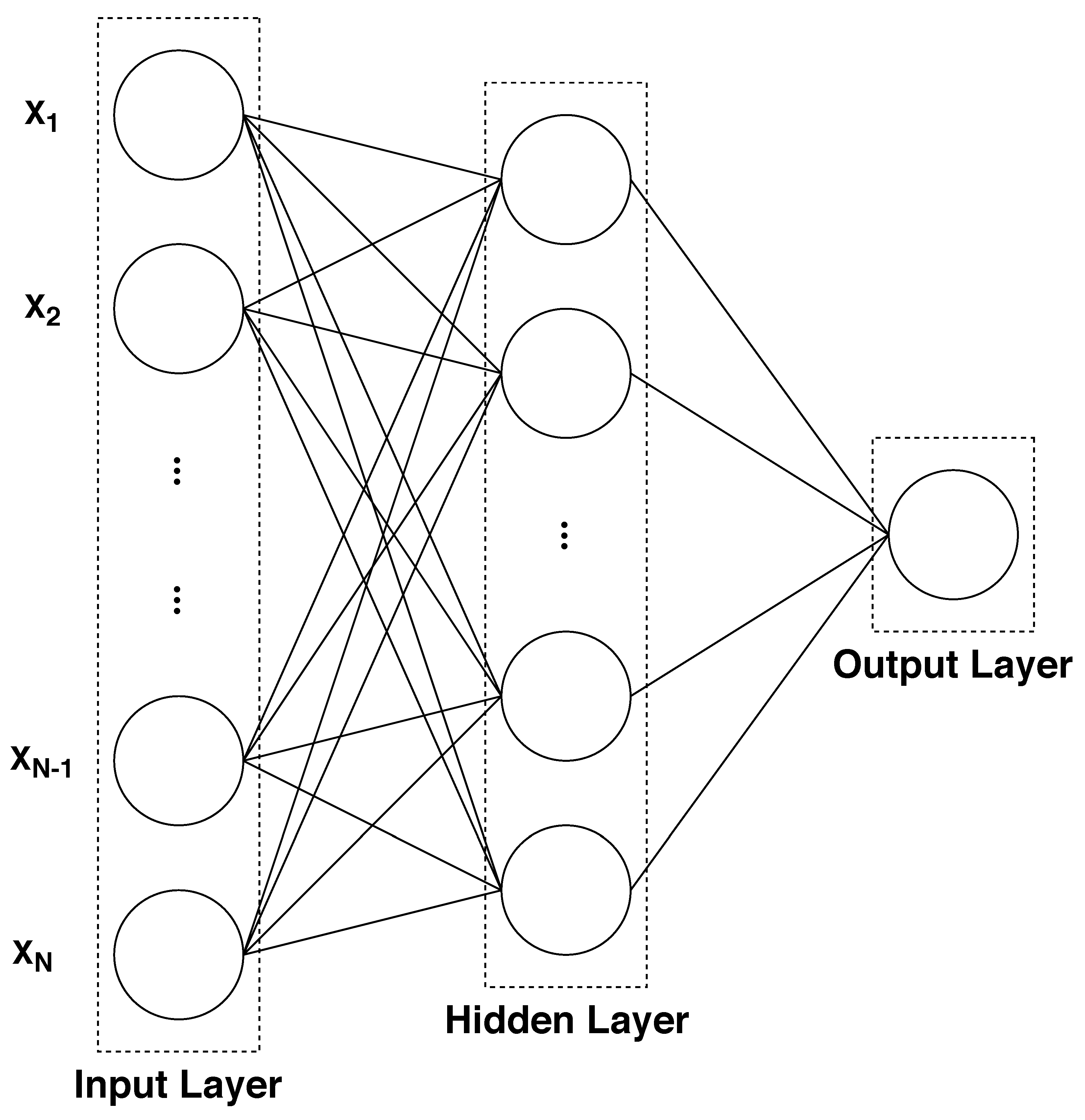
The general structure of the ANN used in this work belongs to the Multilayer Perceptrons class. In particular, the topology of the ANN model we implement, illustrated in Figure 1, consists of an input, a hidden and an output layer. Nodes belonging to the input layer are a large selection of variables (potentially) influencing the outcomes while the output layer consists of only one neuron with a response of zero, representing the event “player i has lost the match”, and one, representing the event “player i has won the match”. According to Hornik (1991), we use only one single hidden layer. This architecture gives good forecasting performances to the model, when the number of nodes included in the hidden layer is sufficiently adequate.

More formally, the ANN structure adopted to forecast the probability of winning of player i in the match j, that is $p_{i,j}$, taking advantage of the set of variables included in ${\mathbf{X}}_j$ operates similarly to a non–linear regression. To simplify the notation, from now on we will always refer to the favourite player (according to Definition 4), such that the suffix identifying player i will disappear, except when otherwise requested. A comprehensive set of notations used in this work is summarized in

Table A1. Suffix identification.

Suffix	Description	Values
i	Player	$i=\left\{f,u\right\}$
j	Match	$j=\left\{1,\cdots ,J\right\}$
$J^L$	Number of matches in the learning sample
$J^{Te}$	Number of matches in the testing sample
$J^{Tr}$	Number of matches in the training sample
$J^V$	Number of matches in the validation sample
n	Variable (potentially) influencing the outcome	$n=\left\{1,\cdots ,N\right\}$
r	Node in the hidden layer	$r=\left\{1,\cdots ,N_h\right\}$
m	ANN model estimated	$m=\left\{1,\cdots ,M\right\}$
k	Professional bookmaker	$k=\left\{1,\cdots ,K\right\}$
t	Day of the match(es)	$t=\left\{1,\cdots ,T\right\}$

. Therefore, let $X_{n,j}\in {\mathbf{X}}_j$ be the nth variable in the match j, potentially influencing the outcome of that match. All the variables in ${\mathbf{X}}_j$, with $j=1,\cdots ,J$, feed the N–dimensional input nodes. Moreover, let $\sigma (·)$ be the transfer or activation function, which in this work is the sigmoid logistic. Therefore, the ANN model with N inputs, one hidden layer having $N_h<N$ nodes and an output layer $Y_j$ is defined as follows:

$$Y_j=\sum _{r=1}^{N_h}{w}_{j,r}\sigma \left(\sum _{n=1}^N{v}_{n,j,r}{X}_{n,j}+{\beta }_r\right),j=1,\dots ,J,$$

(1)

where $w_{j,r}$ represents the weight of the rth hidden neuron, $v_{n,j,r}$ is the weight associated to the nth variable, for the match j and ${\beta }_r$ is the bias vector.

The set-up of the ANN model here employed consists of two distinct steps: A learning and a testing phase. The former uses a dataset of $J^L<J$ matches, and the latter a dataset of $J^{Te}<J^L$ matches, with $J^L+J^{Te}=J$. The learning phase, in turn, encompasses two steps: A training and a validation procedures. In the former phase, the weights of Equation (1) are found on the training sample whose dimension is of $J^{Tr}<J^L$, by means of machine learning algorithms. These learning algorithms find the optimal weights minimizing the error between the desired output provided in the training sample and the actual output computed by the model. The error is evaluated in terms of the Brier Score $\left[BS\right]$:

$$BS=\frac{1}{J}\sum _{j=1}^J{\left(p_j-Y_j\right)}^2.$$

(2)

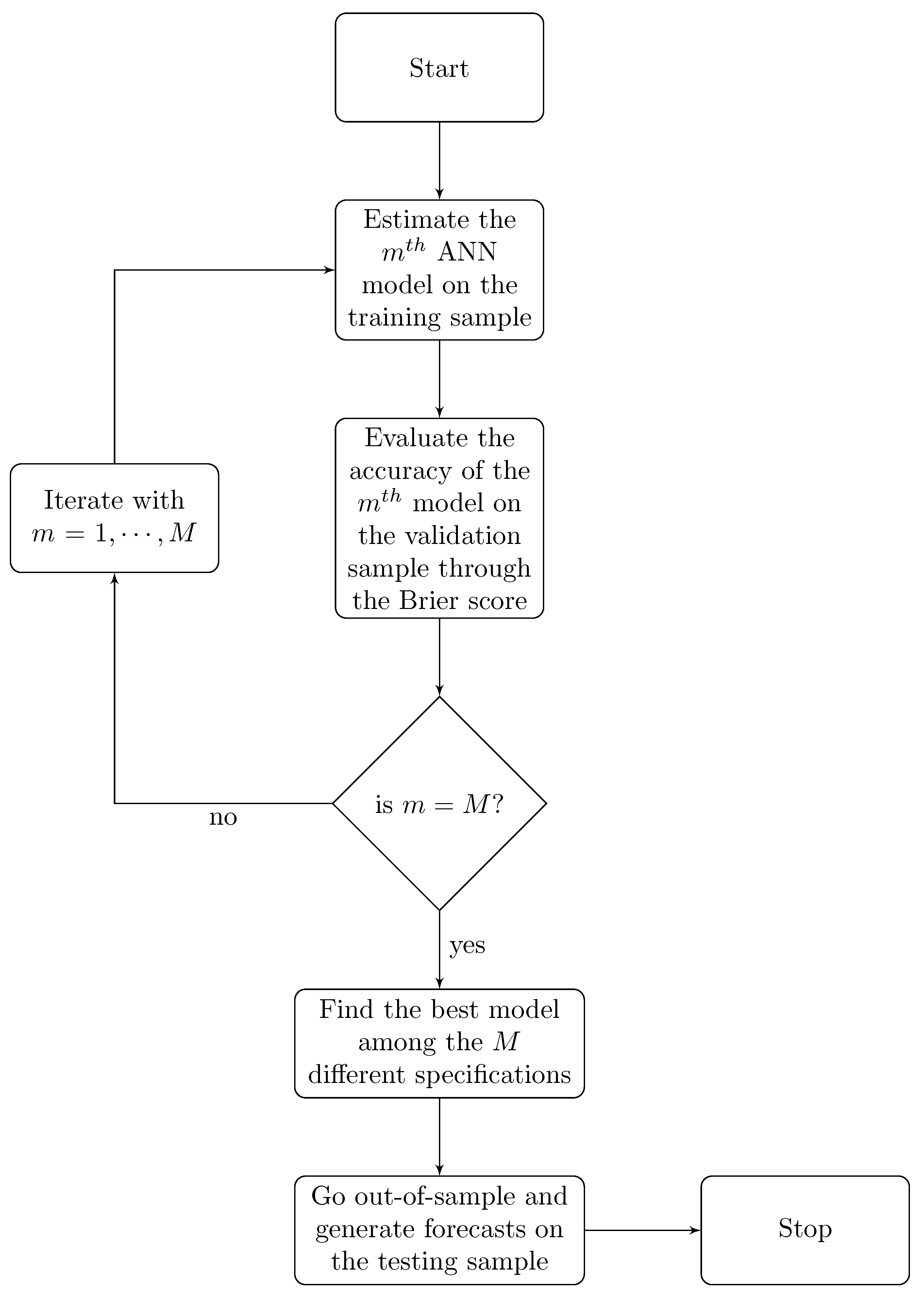
Unfortunately, the performance of such a model highly depends on: (i) The starting values given to the weights in the first step of the estimation routine; (ii) the pre-fixed number of nodes belonging to the hidden layer. To overcome this drawback, a subset of matches $J^V=J^L-J^{Tr}$ is used to evaluate the performance of M different models in a (pseudo) out-of-sample perspective. In other words, M different ANN specifications are estimated, on the basis of several number of nodes belonging to the hidden layer and to decrease the effect of the initial values of the weights. All these M different ANN specifications are evaluated in the validation sample. Once got the optimal weights, that is the weights minimizing Equation (2) for the $J^V$ matches of the learning phase, the resulting specification is used to predict the probability of winning in the testing phase. In such a step, the left-hand side of Equation (1) is replaced by ${\widehat{p}}_j$. A detailed scheme of the overall procedure is presented in Figure 2.

The algorithm used to train the neural network is a feedforward procedure with batch training through the Adam Optimization algorithm (Kingma and Ba 2014). The Adam algorithm, whose name comes out from adaptive moment estimation, consists of an optimization method belonging to the stochastic gradient descent class. Such an algorithm shows better performances with respect to several competitors (as the AdaGrad and RMSprop, mainly in ANN settings with sparse gradients and non–convex optimization, as highlighted by Ruder (2016), among others). More in detail, the Adam algorithm computes adaptive learning rates for each model parameter and has been shown to be efficient in different situations (for instance, when the dataset is very large or when there are many parameters to estimate).

A typical problem affecting the ANNs is the presence of noise in the training set, which may lead to (fragile) models too specialized on the training data. In the related literature, several procedures have been proposed to weaken such a problem, like the dropout (Srivastava et al. 2014) and early stopping (Caruana et al. 2001) approaches. Dropout is a regularization technique consisting of dropping randomly out some neurons from the optimization. As consequence, when some neurons are randomly ignored during the training phase, the remaining neurons will have more influence, giving the model more stability. In the training phase, a $10\%$ dropout regularization rate is used on the hidden layer nodes. The early stopping is a method which helps to determine when the learning phase has to be interrupted. In particular, at the end of each epoch, the validation loss (that is, the $BS$) is computed. If the loss has not improved after two epochs, the learning phase is stopped and the last model is selected.

4. Empirical Application

The software used in this work is R. The R package for the ANN estimation, validation, and testing procedure is keras (Allaire and Chollet 2020). All the codes are available upon request. Data used in this work come from the merge of two different datasets. The first dataset is the historical archive of the site www.tennis-data.co.uk. This archive includes the results of all the most important tennis tournaments (Masters 250, 500 and 1000, Grand Slams and ATP Finals), closing betting odds of different professional bookmakers, ranks, ATP points, and final scores for each player, year by year. The second set of data comes from the site https://github.com/JeffSackmann/tennis_atp. This second archive reports approximately the same set of matches of the first dataset but with some information about the players, such as the handedness, the height, and, more importantly, a large set of statistics in terms of points for each match. For instance, the number of won points on serve, breakpoint saved, aces, and so forth are stored in this dataset. As regards the period under consideration, first matches were played on 4 July 2005 while the most recent matches on 28 September 2018. After the merge of these two datasets, the initial number of matches is 35,042. As said in the Introduction, we aim at configuring an ANN including all the variables employed in the existing approach to estimate the probability of winning in tennis matches. Therefore, after having removed the uncompleted matches (1493) and the matches with missing values in variables used in at least one approach (among the competing specifications LZR, KMR, DCPR, BTM, and BCA), the final dataset reduces to 26,880 matches. All the variables used by each forecasting model are synthetically described in

Table 1. Input variables.

Label	Description	Structural	ANN	LZR	KMR	DCPR	BTM	BCA	Non–Lin. Test
$X_1$	Winning frequency on the first serve		√						2365.875  ***
$X_2$	Winning frequency on the second serve		√						1434.552  ***
$X_3$	Won point return frequency		√						6358.604  ***
$X_4$	Service points won frequency		√						6358.604  ***
$X_5$	Winning frequency on break point		√						574.052  ***
$X_6$	First serve success frequency		√						4.517
$X_7$	Completeness of the player		√						6358.604  ***
$X_8$	Advantage on serving		√						6358.604  ***
$X_9$	Average number of aces per game		√						105.830  ***
$X_{10}$	Minute-based fatigue		√						5.099  *
$X_{11}$	Games-based fatigue		√						3.552
$X_{12}$	Head-to-head		√						20.020  ***
$X_{13}$	ATP Rank	√	√		√				31.793  ***
$X_{14}$	ATP Points	√	√	√					113.887  ***
$X_{15}$	Age	√	√	√		√			3.752
$X_{15sq}$	Squared age	√	√			√			3.525
$X_{16}$	Height	√	√			√			1.208
$X_{16sq}$	Squared height	√	√			√			4.603
$X_{17}$	Surface winning frequency		√						524.558  ***
$X_{18}$	Overall winning frequency		√						165.618  ***
$X_{19}$	Shin implied probability	√	√						0.991
$X_{20}$	Current form of the players		√						4.745  *
$X_{21}$	BT probability		√				√		24.084  ***
$X_{22}$	ATP ranking intervals	√	√	√
$X_{23}$	Home factor	√	√	√
$X_{24}$	BCA winning probability		√					√	1.646
$X_{25}$	Top-10 former presence	√	√			√
$X_{26}$	Both players right-handed	√	√			√
$X_{27}$	Both players left-handed	√	√			√
$X_{28}$	Right-handed fav. and vice versa	√	√			√
$X_{29}$	Left-handed fav. and vice versa	√	√			√
$X_{30}$	Grand Slam match	√	√			√
$X_{31}$	Bookmaker info	√		√					103.681  ***

Notes: The table shows the set of variables included in each model. The column “Structural” identifies if a variable obeys to Definition 3. ANN gives the composition of the proposed artificial neural network, LZR that of the logit regression of Lisi and Zanella (2017); KMR that of the logit regression of Klaassen and Magnus (2003); DCPR that of the probit regression of Del Corral and Prieto-Rodríguez (2010); BTM stands for the BT-type model of McHale and Morton (2011) and BCA for the Barnett and Clarke (2005) point-based approach. The column “Non–lin. test” reports the Teräsvirta test statistics, whose null hypothesis is of “linearity in mean” between Y and each continuous variable. ***, and * denote significance at the 1%, and 10% level, respectively.

, while in the Supplementary Materials, each of them is properly defined. It is worth noting that some variables have been configured with the specific intent of exploring some aspects uncovered by the other approaches, so far. These brand new variables are: $X_1$–$X_{12}$, $X_{17}$, $X_{18}$, and $X_{20}$. For instance, $X_{17}$ and $X_{18}$ take into account the fatigue accumulated by the players, in terms of the time of stay on court and number of games played in the last matches. Moreover, the current form of the player ($X_{20}$) may be a good proxy of the outcome for the upcoming match. This variable considers the current rank of the player with respect to the average rank of the last six months. If the actual ranking is better than the average based on the last six months, then it means that the player is in a good period. The last column of Table 1 reports the test statistics of the non–linearity test of Teräsvirta et al. (1993), which provides a justification for using the ANNs. The null hypothesis of this test is the linearity in mean between the dependent variable (that is, the outcome of the match) and the potential variable influencing this outcome (that is, the variables illustrated in the table). The results of this test, on the basis of all the non–dummy variables included in ${\mathbf{X}}_j$, generally suggest rejecting the linearity hypothesis, corroborating the possibility of using the ANNs to take trace of the emerged non–linearity.

In the learning phase (alternately named in-sample period), each model uses the variables reported in the Table 1 according to the information set ${\mathcal{F}}_j$. In both the learning and testing procedures, with reference to the variables $X_{19}$ and $X_{31}$, we only focus on the odds provided by the professional bookmaker Bet365. The reason for which we use the odds provided by Bet365 is that it presents the largest betting coverage (over 98%) of the whole set of matches. The implied probabilities ($X_{19}$) coming from the Bet365 odds have been normalized according to the procedure proposed by Shin (1991, 1992, 1993). Other normalization techniques are discussed in Candila and Scognamillo (2018).

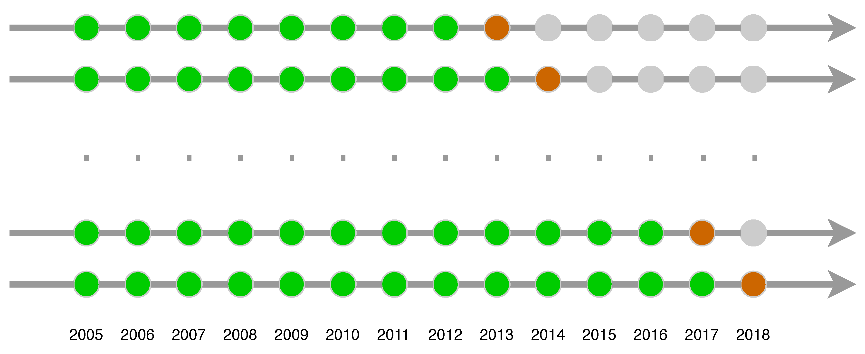
All the models are estimated using six expanding windows, each starting from 2005, and at least composed of 8 years (until 2012). The structure of the resulting procedure is depicted in Figure 3, where the sequence of green circles represents the learning sample and the brown circles the testing (or out-of-sample) periods. Globally, the out-of-sample time span is the period 2013–2018, for a total of 9818 matches. It is worth noting that the final ANN models for each testing year will have a unique set of optimal weights and may also retrieve a different number of nodes belonging to the hidden layer. The ANN models selected by the validation procedure, as illustrated above, have a number of nodes in the hidden layer varying from 5 to 30.

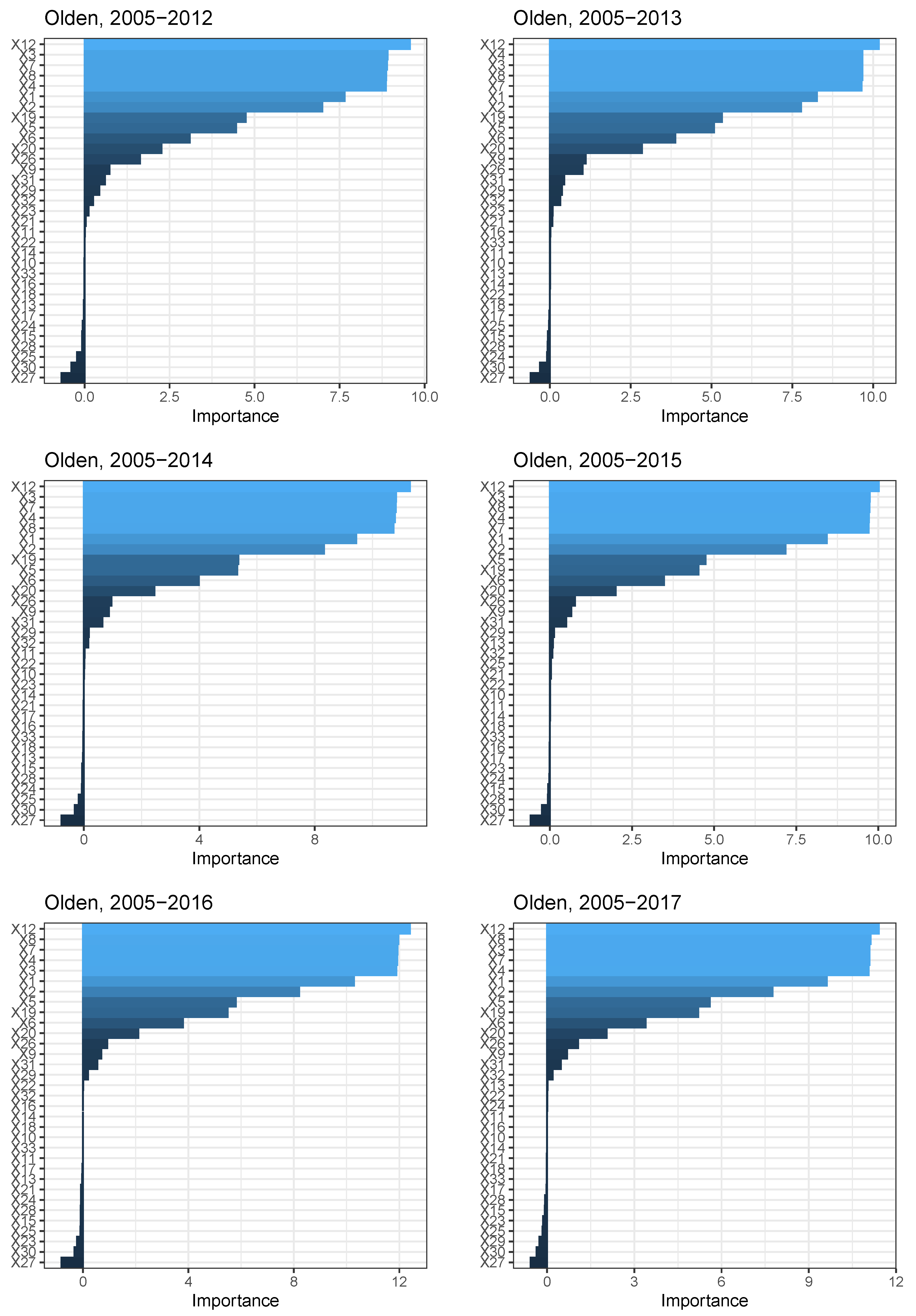
The importance of each input variable, for each learning phase, is depicted in Figure 4, which reports the summed product of the connection weights according to the procedure proposed by Olden et al. (2004). Such a method calculates the variable importance as the product of the raw input-hidden and hidden-output connection weights between each input and output neuron and sums the product across all hidden neurons. Independently of the learning window, the most important variables appear to be $X_{12}$ (Head-to-head), $X_3$ (Won point return frequency), $X_7$ (Completeness of the player), and $X_8$ (Advantage on service).

Out-of-Sample Forecast Evaluation

Once estimated all the models and the ANN for each learning period, the out-of-sample estimates are obtained. When we go out-of-sample, the structural variables are invariant such that no predictions are made for these ones. For all the other variables, instead, we need to forecast the values for each match j using the information set ${\mathcal{F}}_{j|j-1}$. For some variables, like $X_{24}$, the literature proposed a method to forecast them (Barnett and Clarke 2005). For the other variables, we consider either the historical mean of the last year (or less, if that period is unavailable) or the value of the match before. Obviously, a model only based on this predicted information, like the BCA, is expected to perform worse than a model only based on structural variables. The evaluation of the performances of the proposed ANN model with respect to each competing model is employed through the Diebold–Mariano (DM) test, according to version, specifically indicated for binary outcomes, suggested by Gneiting and Katzfuss (2014) (Equation (11)). The DM test statistics with relative significance are reported columns two to five of

Table 2. ANN evaluation with the Diebold–Mariano test.

	# Matches	LZR	KMR	DCPR	BTM	BCA	LZR-ANN
2013	2128	2.02 **	−1.8 *	−1.11	−0.86	−13.3 ***	−3.75 ***
2014	1849	0.91	−2.49 **	−2.71 ***	−1.7 *	−13.52 ***	−2.15 **
2015	1315	−0.48	−3.11 ***	−2.91 ***	−3.46 ***	−9.81 ***	−2.91 ***
2016	1696	0.00	−2.86 ***	−1.97 **	−2.75 ***	−12.39 ***	−2.95 ***
2017	1572	−0.11	−1.15	−1.34	−0.88	−13.55 ***	−1.1
2018	1259	0.66	−1.54	−0.18	−1.66 *	−14.36 ***	−1.44
2013–2018	9818	1.47	−5.24 ***	−4.06 ***	−4.46 ***	−31.41 ***	−5.96 ***

Notes: The table reports the Diebold–Mariano test statistic. Negative values mean that the ANN outperforms the model in column and vice versa. *, ** and *** denote significance at the 10%, 5%, and 1% levels,, respectively.

. It results that the proposed model statistically outperforms all the competing models except the LZR. This holds independently of the specific out-of-sample period. It is interesting to note that the LZR is able to outperform the proposed ANN only in 2013. When the learning sample increases, this superior significance vanishes. Given that, from a statistical point of view, only the model of Lisi and Zanella (2017) has a similar performance to that of the proposed ANN, only the LZR will be used for evaluation purposes in the following section dedicated to the betting strategy. Note that the ANN model includes the same set of variables of the LZR, except for variable $X_{31}$ (see Table 1). Therefore, it would be worthy of investigation performing an additional analysis between the proposed (full) ANN model and a restricted ANN specification, based only on the variables of the LZR. We label this model as “LZR-ANN”. The resulting evaluation is illustrated in the last column of Table 2, where again the DM test statistics are reported. Interestingly, the full ANN model largely outperforms the restricted LZR-ANN, signalling the importance of including as many as possible input variables in the ANN model.

5. Betting Strategies

As said before, the variables related to the bookmaker odds used in the learning and testing phases were those provided by Bet365. However, for the same match different odds provided by other professional bookmakers are available. Therefore, let $o_{i,k,j}$ be the odds provided by the bookmaker k for the player i and the match j, with $k=1,\cdots ,K$. Then, the definition of the best odds is provided:

Definition 5.

The best odds for player i and the match j, denoted with $o_{i,j}^{Best}$, is the maximum value among the K available odds for the match j. Formally:

$$o_{i,j}^{Best}=\underset{k=1,\dots ,K}{max}{o}_{i,k,j}.$$

Let ${\widehat{p}}_{i,j}$ be the estimated probability obtained from the proposed ANN or the LZR for the player i and the match j, for the out-of-sample matches (the period 2013–2018). Let us focus on the probabilities for the favourites ${\widehat{p}}_{f,j}$. If these probabilities are high, the model (ANN or LZR) gives high chances to the favourite to win the match. Otherwise, low probabilities ${\widehat{p}}_{f,j}$ imply that the model signals the other player as the true favourite. From an economic point of view, it is convenient to choose a threshold above which a bet is placed on the favourite, and below which a bet is placed on the underdog. High thresholds will imply a smaller number of bets, but with greater chances for that player to win the match. These thresholds are based on the sample quantiles of the estimated probabilities, according to the following definitions:

Definition 6.

Let $P_f$ and $P_u$ be all the estimated probabilities for a particular (out-of-sample) period, for the favourite and underdog players, respectively.

Definition 7.

Let $q\left(\alpha \right)$ be the sample quantile corresponding to the probability α, that is: $Pr(P_f\le q\left(\alpha \right))=\alpha$ or $Pr(P_u\le q\left(\alpha \right))=\alpha$.

So far, we have only identified the jth match among the total number of matches played. However, for the setting of some betting strategies, it is useful to refer the match j to the day t, by the following definitions:

Definition 8.

Let $j\left(t\right)$ and $J\left(t\right)$ be, respectively, the jth and the total number of matches played in the day t. Assuming that $t=1,\cdots ,T$, the total number of matches played is $J={\sum }_{t=1}^{T}J\left(t\right)$.

Definition 9.

Let ${\widehat{p}}_{f,j\left(t\right)}^{st}$, ${\widehat{p}}_{f,j\left(t\right)}^{nd}$, ${\widehat{p}}_{u,j\left(t\right)}^{st}$ and ${\widehat{p}}_{u,j\left(t\right)}^{nd}$ be the estimated top-2 probabilities (following Definition (5)) for the favourite and underdog (according to Definition 4) among all the $J\left(t\right)$ matches played on day t, respectively.

Finally, the best odds, that is the highest odds on the basis of Definition 5, whose estimated probabilities follow Definition 9 are defined as:

Definition 10.

According to Definitions 5 and 8, let $o_{i,j\left(t\right)}^{Best,st}$ and $o_{i,j\left(t\right)}^{Best,nd}$ be the best odds for player i associated to the matches played on day t satisfying Definition 9.

The four proposed betting strategies are synthetically denoted by $S_1$, $S_2$, $S_3$ and $S_4$. The first two strategies produce gains (or losses) coming from single bets. In this case, an outcome for the match j successfully predicted is completely independent of another outcome, always correctly predicted. Therefore, from an economic viewpoint, the gains coming from two successful bets are equal to the sum of every single bet. However, it is also possible to obtain larger gains if two events are jointly considered in a single bet. In this circumstance, the gains will be obtained from the multiplications (and not from the summation) of the odds. The strategies $S_3$ and $S_4$ take advantage of this aspect. In particular, they allow to jointly bet on two matches for each day t, at most. Therefore, $S_3$ and $S_4$ may be more remunerative than betting on a single event but are much riskier, because they yield some gains only if both the events forming the single bet are correctly predicted. All the strategies will select the matches to bet on the basis of different sample quantiles depending on $\alpha$ (see Definition 7). For example, let $\alpha$ be close to one. In the case of betting on the favourites, only the probabilities ${\widehat{p}}_{f,j}$ with very high values will be selected. That is, only the matches in which the winning of the favourite player is retained almost sure will be suggested. The same but with opposite meaning will hold for those matches whose estimated probabilities ${\widehat{p}}_{f,j}$ are below to a sample quantile when $\alpha$ is close to zero. The message here is that the model (ANN or the competing specification) signals the favourite player (according to Definition 4) as a potential defeated player, such that it would be more convenient to bet on the adversary.

5.1. Strategy $S_1$

The strategy $S_1$ suggests to bet one dollar on the favourite, according to the Definition 4, in the match j if and only if ${\widehat{p}}_{f,j}\ge q\left(\alpha \right)$. The returns of the strategy $S_1$, labelled as $R_{f,j}^{S_1}$ are:

$$R_{f,j}^{S_1}=\{\begin{array}{}\mathrm{(3a)}& o_{f,j}^{Best}-1\hspace{0.17em}\hspace{0.17em}\mathrm{if}\hspace{0.17em}\mathrm{player}\hspace{0.17em}f\hspace{0.17em}\mathrm{wins};\mathrm{(3b)}& -1\hspace{0.17em}\hspace{0.17em}\mathrm{if}\hspace{0.17em}\mathrm{player}\hspace{0.17em}f\hspace{0.17em}\mathrm{loses}.\end{array}$$

The strategy $S_1$ suggests to bet one dollar on the underdog, according to the Definition 4, in the match j if and only if ${\widehat{p}}_{f,j}<q\left(\alpha \right)$. In this case, the returns, labelled as $R_{u,j}^{S_1}$ are:

$$R_{u,j}^{S_1}=\{\begin{array}{}\mathrm{(4a)}& o_{u,j}^{Best}-1\hspace{0.17em}\hspace{0.17em}\mathrm{if}\hspace{0.17em}\mathrm{player}\hspace{0.17em}u\hspace{0.17em}\mathrm{wins};\mathrm{(4b)}& -1\hspace{0.17em}\hspace{0.17em}\mathrm{if}\hspace{0.17em}\mathrm{player}\hspace{0.17em}u\hspace{0.17em}\mathrm{loses}.\end{array}$$

5.2. Strategy $S_2$

The strategy $S_2$, contrary to $S_1$, suggests to bet the amount $o_{f,j}^{Best}$ on the favourite (always satisfying Definition 4) in the match j if and only if ${\widehat{p}}_{f,j}\ge q\left(\alpha \right)$. The returns of $S_2$ for the favourite are labelled as $R_{f,j}^{S_2}$ and are:

$$R_{f,j}^{S_2}=\{\begin{array}{}\mathrm{(5a)}& (o_{f,j}^{Best}-1)o_{f,j}^{Best}\hspace{0.17em}\hspace{0.17em}\mathrm{if}\hspace{0.17em}\mathrm{player}\hspace{0.17em}f\hspace{0.17em}\mathrm{wins};\mathrm{(5b)}& -o_{f,j}^{Best}\hspace{0.17em}\hspace{0.17em}\mathrm{if}\hspace{0.17em}\mathrm{player}\hspace{0.17em}f\hspace{0.17em}\mathrm{loses}.\end{array}$$

The amount $o_{u,j}^{Best}$ is placed on the underdog satisfying Definition 4 in the match j if and only if ${\widehat{p}}_{f,j}<q\left(\alpha \right)$. The returns of such a strategy $R_{u,j}^{S_2}$ are:

$$R_{u,j}^{S_2}=\{\begin{array}{}\mathrm{(6a)}& (o_{u,j}^{Best}-1)o_{u,j}^{Best}\hspace{0.17em}\hspace{0.17em}\mathrm{if}\hspace{0.17em}\mathrm{player}\hspace{0.17em}u\hspace{0.17em}\mathrm{wins};\mathrm{(6b)}& -o_{u,j}^{Best}\hspace{0.17em}\hspace{0.17em}\mathrm{if}\hspace{0.17em}\mathrm{player}\hspace{0.17em}u\hspace{0.17em}\mathrm{loses}.\end{array}$$

5.3. Strategy $S_3$

For the favourite on the basis of Definition 4, $S_3$ suggests to bet one dollar on the top-2 matches of day t both satisfying Definition 9 and the conditions ${\widehat{p}}_{f,j\left(t\right)}^{st}\ge q\left(\alpha \right)$ and ${\widehat{p}}_{f,j\left(t\right)}^{nd}\ge q\left(\alpha \right)$. The returns for the day t, labelled as $R_{f,t}^{S_3}$, are:

$$R_{f,t}^{S_3}=\{\begin{array}{}\mathrm{(7a)}& o_{f,j\left(t\right)}^{Best,st}·o_{f,j\left(t\right)}^{Best,nd}-1\hspace{0.17em}\hspace{0.17em}\mathrm{if}\hspace{0.17em}\mathrm{both}\hspace{0.17em}\mathrm{players}\hspace{0.17em}f\hspace{0.17em}\mathrm{win};\mathrm{(7b)}& -1\hspace{0.17em}\hspace{0.17em}\mathrm{if}\hspace{0.17em}\mathrm{at}\hspace{0.17em}\mathrm{least}\hspace{0.17em}\mathrm{one}\hspace{0.17em}\mathrm{player}\hspace{0.17em}f\hspace{0.17em}\mathrm{loses}.\end{array}$$

For the underdog selected by Definition 4, $S_3$ suggests to bet one dollar on the top-2 matches of day t both satisfying Definition 9 and the conditions ${\widehat{p}}_{f,j\left(t\right)}^{st}<q\left(\alpha \right)$ and ${\widehat{p}}_{f,j\left(t\right)}^{nd}<q\left(\alpha \right)$. The returns for the day t, labelled as $R_{u,t}^{S_3}$, are:

$$R_{u,t}^{S_3}=\{\begin{array}{}\mathrm{(8a)}& o_{u,j\left(t\right)}^{Best,st}·o_{u,j\left(t\right)}^{Best,nd}-1\hspace{0.17em}\hspace{0.17em}\mathrm{if}\hspace{0.17em}\mathrm{both}\hspace{0.17em}\mathrm{players}\hspace{0.17em}u\hspace{0.17em}\mathrm{win};\mathrm{(8b)}& -1\hspace{0.17em}\hspace{0.17em}\mathrm{if}\hspace{0.17em}\mathrm{at}\hspace{0.17em}\mathrm{least}\hspace{0.17em}\mathrm{one}\hspace{0.17em}\mathrm{player}\hspace{0.17em}u\hspace{0.17em}\mathrm{loses}.\end{array}$$

5.4. Strategy $S_4$

The strategy $S_4$ for the favourite suggests to bet the amount $\left(o_{f,j\left(t\right)}^{Best,st}·o_{f,j\left(t\right)}^{Best,nd}\right)$ on the top-2 matches of day t both satisfying Definition 9 and the conditions ${\widehat{p}}_{f,j\left(t\right)}^{st}\ge q\left(\alpha \right)$ and ${\widehat{p}}_{f,j\left(t\right)}^{nd}\ge q\left(\alpha \right)$. The returns for the day t, labelled as $R_{f,t}^{S_4}$, are:

$$R_{f,t}^{S_4}=\{\begin{array}{}\mathrm{(9a)}& (o_{f,j\left(t\right)}^{Best,st}·o_{f,j\left(t\right)}^{Best,nd}-1)o_{f,j\left(t\right)}^{Best,st}·o_{f,j\left(t\right)}^{Best,nd}\hspace{0.17em}\hspace{0.17em}\mathrm{if}\hspace{0.17em}\mathrm{both}\hspace{0.17em}\mathrm{players}\hspace{0.17em}f\hspace{0.17em}\mathrm{win};\mathrm{(9b)}& -o_{f,j\left(t\right)}^{Best,st}·o_{f,j\left(t\right)}^{Best,nd}\hspace{0.17em}\hspace{0.17em}\mathrm{if}\hspace{0.17em}\mathrm{at}\hspace{0.17em}\mathrm{least}\hspace{0.17em}\mathrm{one}\hspace{0.17em}\mathrm{player}\hspace{0.17em}f\hspace{0.17em}\mathrm{loses}.\end{array}$$

Finally, the strategy $S_4$ for the underdog suggests to bet the amount $\left(o_{u,j\left(t\right)}^{Best,st}·o_{u,j\left(t\right)}^{Best,nd}\right)$ on the top-2 matches of day t both satisfying Definition 9 and the conditions ${\widehat{p}}_{f,j\left(t\right)}^{st}<q\left(\alpha \right)$ and ${\widehat{p}}_{f,j\left(t\right)}^{nd}<q\left(\alpha \right)$. The returns for the day t, labelled as $R_{u,t}^{S_4}$, are:

$$R_{u,t}^{S_4}=\{\begin{array}{}\mathrm{(10a)}& (o_{u,j\left(t\right)}^{Best,st}·o_{u,j\left(t\right)}^{Best,nd}-1)o_{u,j\left(t\right)}^{Best,st}·o_{u,j\left(t\right)}^{Best,nd}\hspace{0.17em}\hspace{0.17em}\mathrm{if}\hspace{0.17em}\mathrm{both}\hspace{0.17em}\mathrm{players}\hspace{0.17em}u\hspace{0.17em}\mathrm{win};\mathrm{(10b)}& -o_{u,j\left(t\right)}^{Best,st}·o_{u,j\left(t\right)}^{Best,nd}\hspace{0.17em}\hspace{0.17em}\mathrm{if}\hspace{0.17em}\mathrm{at}\hspace{0.17em}\mathrm{least}\hspace{0.17em}\mathrm{one}\hspace{0.17em}\mathrm{player}\hspace{0.17em}u\hspace{0.17em}\mathrm{loses}.\end{array}$$

5.5. Return-On-Investment (ROI)

The ROI obtained from a given strategy is calculated as the ratio between the sum of the returns as previously defined and the amount of money invested. Let $B_i^{S_l}$ be the total number of bets placed on player i, with $i=\left\{f,u\right\}$, according to the strategy $S_l$, with $l=\left\{1,2,3,4\right\}$. Moreover, let $EX{P}_{i,j}^{S_l}$ be the amount of money invested on betting on player i, according to strategy $S_l$, in the match j. In other words, $EX{P}_{i,j}^{S_l}$ is nothing else that the summation of the quantities reported in Equations (3b), (5b), (7b) and (9b) for the bets on the favourite and in Equations (4b), (6b), (8b) and (10b) for the bets on the underdogs. The ROI for the player i and the strategy $S_l$, expressed in percentage, labelled as ROI${}_i^{S_l}$, is given by:

$${\mathrm{ROI}}_i^{S_l}=100\frac{{\sum }_{j=1}^{B_i^{S_l}}{R}_{i,j}^{S_l}}{{\sum }_{j=1}^{B_i^{S_l}}\left|EX{P}_{i,j}^{S_l}\right|},\mathrm{with}i=\left\{f,u\right\}\mathrm{and}l=\left\{1,2,3,4\right\}.$$

(11)

Note that when the strategies $S_3$ and $S_4$ are employed, the calculation of the ROI through Equation (11) requires the substitution of j with t. The ROI can be positive or negative, depending on the numerator of Equation (11). In the first case, it means that the strategy under investigation has yielded positive returns. Otherwise, the strategy has lead to some losses.

The ROIs for all the strategies, according to different values of the probability $\alpha$ used to calculate the quantile $q\left(\alpha \right)$, for the ANN and LZR methods and for the favourite and underdog players are reported in Panels A of

Table 3. ANN and LZR ROI (in %) for betting on favourites.

	ANN	LZR	ANN	LZR	ANN	LZR	ANN	LZR
	$\alpha =0.5$		$\alpha =0.75$		$\alpha =0.90$		$\alpha =0.95$
	Panel A: All matches
$S_1$	−1.63	−2.67	−0.96	−1.13	−0.89	−1.60	0.79	−1.00
$S_2$	−1.72	−3.52	0.60	0.50	3.69	2.83	10.41	8.57
$S_3$	−8.29	−9.82	−5.31	−4.85	−0.94	−2.21	0.76	−1.47
$S_4$	−10.01	−12.84	−6.26	−6.29	4.73	3.45	10.41	8.68
# Bets	4907	4907	2455	2455	984	984	493	493
	Panel B: Grand Slam matches
$S_1$	1.13	0.59	1.41	1.36	−0.15	−1.35	−0.58	−3.20
$S_2$	1.29	0.33	1.69	1.84	0.18	−1.53	−0.60	−3.36
$S_3$	−1.67	−2.76	−1.11	0.32	−0.36	−2.97	−0.62	−3.40
$S_4$	−2.21	−3.22	−1.06	0.93	0.14	−3.33	−0.52	−3.46
# Bets	1064	1069	594	611	290	278	158	161
	Panel C: Matches with a top-50 as favourite
$S_1$	−1.74	−2.64	−0.95	−1.13	−0.89	−1.60	0.79	−1.00
$S_2$	−1.90	−3.47	0.63	0.50	3.69	2.83	10.41	8.57
$S_3$	−7.69	−9.77	−5.38	−4.85	−0.94	−2.21	0.76	−1.47
$S_4$	−9.43	−12.81	−6.35	−6.29	4.73	3.45	10.41	8.68
# Bets	4800	4871	2453	2455	984	984	493	493
	Panel D: Matches in the first six months
$S_1$	−0.59	−2.19	−0.54	−0.29	−0.64	−1.67	−0.13	−1.63
$S_2$	0.13	−2.62	2.07	2.40	6.34	4.99	14.20	11.84
$S_3$	−7.78	−10.30	−4.84	−5.21	−1.37	−3.49	−0.43	−2.59
$S_4$	−10.35	−13.80	−5.86	−7.06	7.06	4.80	13.44	11.46
# Bets	3266	3248	1653	1688	675	681	330	349

Notes: The table shows the ROI for the ANN and LZR methods, on the basis of four different betting strategies $S_1$, $S_2$, $S_3$, and $S_4$. The bets are all placed on the favourite(s), according to Definition 4. # Bets represents the number of bets placed. The out-of-sample period consists of all the 9818 matches played from 2013 to 2018.

and

Table 4. ANN and LZR ROI (in %) for betting on underdogs.

	ANN	LZR	ANN	LZR	ANN	LZR	ANN	LZR
	$\alpha =0.5$		$\alpha =0.25$		$\alpha =0.10$		$\alpha =0.05$
	Panel A: All matches
$S_1$	−0.32	−4.47	−0.92	−5.22	0.21	−4.17	1.65	−1.75
$S_2$	−5.50	−13.07	−5.99	−9.11	2.46	−7.14	5.16	−3.27
$S_3$	−2.50	−4.44	−1.47	−1.93	5.09	−6.04	1.93	−3.88
$S_4$	−2.65	0.25	−0.75	7.24	26.40	−8.00	7.68	−5.32
# Bets	4907	4907	2455	2455	984	984	493	493
	Panel B: Grand Slam and Masters 1000 matches
$S_1$	−1.10	−5.89	−0.45	−7.71	2.30	−6.48	−0.31	0.87
$S_2$	−3.08	−9.12	−3.67	−6.64	19.55	−10.80	1.94	1.20
$S_3$	6.93	0.05	14.94	2.91	15.59	−3.64	1.18	3.72
$S_4$	22.89	30.78	40.28	35.23	79.51	−1.52	13.02	3.03
# Bets	1646	1677	837	856	371	353	202	170
	Panel C: Matches with a top-50 as underdog
$S_1$	2.76	−3.40	3.81	−3.26	3.16	−6.48	4.69	−12.98
$S_2$	9.68	0.31	6.57	7.83	9.94	−9.95	17.00	−20.05
$S_3$	3.98	−9.43	4.54	−4.18	6.49	−9.68	6.49	−13.85
$S_4$	2.82	5.30	2.86	−2.39	10.70	−10.02	19.19	−15.52
# Bets	1633	1282	1092	733	619	291	367	136
	Panel D: Matches in the first six months
$S_1$	−2.92	−7.78	−3.55	−8.32	−0.19	−4.47	−0.64	−0.27
$S_2$	−11.40	−21.23	−10.23	−16.90	6.57	−7.59	5.00	−0.35
$S_3$	−13.16	−10.57	−9.26	−6.77	2.60	−7.38	0.52	−2.47
$S_4$	−9.02	−1.88	−4.08	6.14	37.60	−9.08	12.39	−3.50
# Bets	3206	3224	1635	1636	657	677	343	356

Notes: The table shows the ROI for the ANN and LZR methods, on the basis of four different betting strategies $S_1$, $S_2$, $S_3$, and $S_4$. The bets are all placed on the underdog(s), according to Definition 4. # Bets represents the number of bets placed. The out-of-sample period consists of all the 9818 matches played from 2013 to 2018.

, respectively. The same tables report the ROIs for a number of subsets of matches, for robustness purposes (Panel B to Panel D). Several points can be underlined looking at Panels A. First, note that when $\alpha =0.5$, the quantile corresponds to the median. In this case, all the 9818 matches forming the out-of-sample datasets (from 2013 to 2018) are equally divided in bets on the favourites and underdogs. Obviously, betting on all the matches is never a good idea: Independently of the strategy adopted, the ROIs coming from betting on the favourites are always negative. However, those obtained from the matches selected by the ANN model are less negative than those obtained from the LZR. For instance, according to strategy $S_4$, the losses for the ANN model are equal to 10.01% of the invested capital, while for the LZR are equal to 12.84%. The occurrence of negative returns in betting markets has been largely investigated in the literature. In terms of expected values, there are positive and negative returns according to the type of bettors. As pointed out by Coleman (2004), there exists a group of skilled or informed bettors, which placing low odds bets have a positive or near zero expected returns. Then, another group of bettors, defined as risk lovers, being less skilled or informed compared to the first group, place bets mainly on longer odds bets. This group of bettors has negative expected returns. Therefore, also negative returns are perfectly consistent with betting markets. Second, the number of matches largely decreases when the probability $\alpha$ increases (for Table 3) or decreases (for Table 4). When the bets are placed only on the matches with a well-defined favourite (that is, ${\widehat{p}}_{f,j}\ge q\left(\alpha \right)$, with $\alpha =0.95$), the ROIs become positive. Considering the last two columns of Panel A for Table 3, independently of the strategy adopted, the ROIs of the ANN model are always positive and bigger than those of the LRZ method. Betting on the underdogs when the estimated probability for the favourite is below the smallest quantile considered ($\alpha =0.05$) lets again positive ROIs, but this time only for the ANN (last two columns of the Panel A for Table 4). Summarizing the results exposed in both the top panels of Table 3 and Table 4, it appears clear that among the sixteen considered set of bets, the ANN model outperforms the competing model fifteen times for bets on the favourites (only under $S_3$ and $\alpha =0.75$ the losses are greater for the ANN model) and fourteen times for bets on the underdogs (under $S_4$ and $\alpha =0.5$ and $\alpha =0.25$ the LZR specification reports positive ROIs while the ANN model reports negative results).

Given these prominent achievements, the robustness of these ROIs obtained using the probability of winning estimated by the implemented ANN is extensively evaluated. This issue is addressed by restricting the set of matches to bet on according to three different criteria, shown in Panels B to D of Table 3 and Table 4. More in detail, for bets on the favourites and underdogs only the matches played in Grand Slams and in Grand Slams and Masters 1000 are, respectively, selected (Panels B). Panels C depict the ROIs for the bets on matches with a top-50 as favourite (Table 3) or with a top-50 as underdog (Table 4). Finally, Panels D show the ROIs with respect to the matches only played in the first six months of each year. Again, the ROIs of the proposed model are generally better, sometimes much better than the corresponding ROIs of the LZR. For instance, betting on the underdogs with the sample quantile chosen for $\alpha =0.10$ and the strategy $S_4$ lets a ROI of 79.51% for the ANN and losses of 1.52% of the capital invested for the LZR.

To conclude, even if from a statistical point of view the out-of-sample performance of the ANN is not different from that of the LZR, from an economic viewpoint, the results of the proposed model are very encouraging. Irrespective of the betting strategy adopted, the chosen quantile used to select the matches to bet on, the subset of matches (if all the out-of-sample matches, or a smaller set on the basis of three alternative criteria), the ROIs guaranteed by the ANN are almost always better than those obtained from the LZR method.

6. Conclusions

The ultimate goals of a forecasting model aiming at predicting the probability of winning of a team/player before the beginning of the match are: Robustly beating the existing approaches from a statistical and economic point of view. This contribution attempted to pursue both these objectives, in the context of male tennis. So far, three main categories of forecasting models are available within this context: Regression-based, point-based, and paired-based approaches. Each method differs from the other not only for the different statistical methodologies applied (for instance, probit or logit for the regression-based approach, BT-type model for the paired-based specification, and so forth) but also for the different variables influencing the outcome of the match considered. This latter aspect highlights that several variables can potentially influence the result of the matches, and taking all of them into consideration may be problematic, mainly in the parametric model, such as the standard regressions. In this framework, we investigate the possibility of using the ANNs with a variety of input variables. More in detail, the design of the proposed ANN consists of a feed-forward rule trained by backpropagation, with Adam algorithm incorporated in the optimization procedure. As regards the input nodes, some variables come from a selection of the existing approaches aimed at forecasting the winner of the match, while some other variables are intentionally created for the purpose of taking into account some aspects uncovered by the other approaches. For instance, variables handling the players’ fatigue both in terms of minutes and in terms of games played are configured. Five models belonging to the previously cited approaches constitute the competing specifications. From a statistical point of view, the proposed configuration of the ANN beats four out of five competing approaches while it is at least as good as the regression model labelled as LZR, proposed by Lisi and Zanella (2017). In order to provide help in the complicated issue of the matches’ choice on which placing a bet, four betting strategies are proposed. The chosen matches derive from the overcoming of the estimated probability sample quantiles. Higher quantiles imply fewer matches on which place a bet and vice versa. Moreover, two of these strategies suggest to jointly bet on the two matches played in a day whose estimated probabilities are the most confident, among all the available probabilities of that day, towards the two players. These two strategies assure higher returns at the price of being riskier because they depend on the outcomes of two matches. In comparing the ROIs of the ANN with those of the LRZ obtained from the four betting strategies proposed, it results that the ANN model implemented guarantees higher, sometimes much higher, net returns than those of the LZR. These superior ROIs are achieved irrespectively of the choice of the player to bet on (if favourite or underdog) and of the subset of matches selected according to three different criteria.

Further research may be related to the extension of the ANN tools to other sports. Moreover, the four proposed betting strategies could be applied to other disciplines, taking advantage of the market inefficiencies (see the contribution of Cortis et al. (2013) for the inefficiency in the soccer betting market, for instance).

References

- Allaire, Joseph J., and François Chollet. 2020. Keras: R Interface to ’Keras’, (R package version 2.3.0.0).
- Allen, David E, Michael McAleer, Shelton Peiris, and Abhay K. Singh. 2016. Nonlinear time series and neural-network models of exchange rates between the US dollar and major currencies. Risks 4: 7. [Google Scholar] [CrossRef] [Green Version]
- Atsalakis, George S., Ioanna G. Atsalaki, and Constantin Zopounidis. 2018. Forecasting the success of a new tourism service by a neuro-fuzzy technique. European Journal of Operational Research 268: 716–27. [Google Scholar] [CrossRef]
- Barnett, T., A. Brown, and S. Clarke. 2006. Developing a model that reflects outcomes of tennis matches. Paper presented at 8th Australasian Conference on Mathematics and Computers in Sport, Coolangatta, Australia, July 3–5; pp. 178–88. [Google Scholar]
- Barnett, Tristan, and Stephen R. Clarke. 2005. Combining player statistics to predict outcomes of tennis matches. IMA Journal of Management Mathematics 16: 113–20. [Google Scholar] [CrossRef]
- Boulier, Bryan L., and Herman O. Stekler. 1999. Are sports seedings good predictors? An evaluation. International Journal of Forecasting 15: 83–91. [Google Scholar] [CrossRef]
- Brier, Glenn W. 1950. Verification of forecasts expressed in terms of probability. Monthly Weather Review 78: 1–3. [Google Scholar] [CrossRef]
- Candila, Vincenzo, and Antonio Scognamillo. 2018. Estimating the implied probabilities in the tennis betting market: A new normalization procedure. International Journal of Sport Finance 13: 225–42. [Google Scholar]
- Cao, Qing, Bradley T. Ewing, and Mark A. Thompson. 2012. Forecasting wind speed with recurrent neural networks. European Journal of Operational Research 221: 148–54. [Google Scholar] [CrossRef]
- Caruana, Rich, Steve Lawrence, and C. Lee Giles. 2001. Overfitting in neural nets: Backpropagation, conjugate gradient, and early stopping. In Advances in Neural Information Processing Systems. Cambridge: MIT Press, pp. 402–8. [Google Scholar]
- Clarke, Stephen R., and David Dyte. 2000. Using official ratings to simulate major tennis tournaments. International Transactions in Operational Research 7: 585–94. [Google Scholar] [CrossRef]
- Coleman, Les. 2004. New light on the longshot bias. Applied Economics 36: 315–26. [Google Scholar] [CrossRef]
- Condon, Edward M., Bruce L. Golden, and Edward A. Wasil. 1999. Predicting the success of nations at the Summer Olympics using neural networks. Computers & Operations Research 26: 1243–65. [Google Scholar]
- Cortis, Dominic, Steve Hales, and Frank Bezzina. 2013. Profiting on inefficiencies in betting derivative markets: The case of UEFA Euro 2012. Journal of Gambling Business & Economics 7: 41–53. [Google Scholar]
- Del Corral, Julio, and Juan Prieto-Rodríguez. 2010. Are differences in ranks good predictors for Grand Slam tennis matches? International Journal of Forecasting 26: 551–63. [Google Scholar] [CrossRef]
- Gneiting, Tilmann, and Matthias Katzfuss. 2014. Probabilistic forecasting. Annual Review of Statistics and Its Application 1: 125–51. [Google Scholar] [CrossRef]
- Hassanniakalager, Arman, and Philip W. S. Newall. 2019. A machine learning perspective on responsible gambling. Behavioural Public Policy, 1–24. [Google Scholar] [CrossRef] [Green Version]
- Haykin, Simon. 2009. Neural Networks and Learning Machines, 3rd ed. Upper Saddle River: Pearson Education. [Google Scholar]
- Hornik, Kurt. 1991. Approximation capabilities of multilayer feedforward networks. Neural Networks 4: 251–57. [Google Scholar] [CrossRef]
- Hucaljuk, Josip, and Alen Rakipović. 2011. Predicting football scores using machine learning techniques. In Paper presented at 2011 Proceedings of the 34th International Convention MIPRO, Opatija, Croatia, May 23–27; pp. 1623–27. [Google Scholar]
- Jain, Ashu, and Avadhnam Madhav Kumar. 2007. Hybrid neural network models for hydrologic time series forecasting. Applied Soft Computing 7: 585–92. [Google Scholar] [CrossRef]
- Kingma, Diederik P., and Jimmy Ba. 2014. Adam: A method for stochastic optimization. arXiv arXiv:1412.6980. [Google Scholar]
- Klaassen, Franc J.G.M., and Jan R. Magnus. 2003. Forecasting the winner of a tennis match. European Journal of Operational Research 148: 257–67. [Google Scholar] [CrossRef] [Green Version]
- Knottenbelt, William J., Demetris Spanias, and Agnieszka M Madurska. 2012. A common-opponent stochastic model for predicting the outcome of professional tennis matches. Computers & Mathematics with Applications 64: 3820–27. [Google Scholar]
- Kovalchik, Stephanie Ann. 2016. Searching for the GOAT of tennis win prediction. Journal of Quantitative Analysis in Sports 12: 127–38. [Google Scholar] [CrossRef] [Green Version]
- Liestbl, Knut, Per Kragh Andersen, and Ulrich Andersen. 1994. Survival analysis and neural nets. Statistics in Medicine 13: 1189–200. [Google Scholar] [CrossRef] [PubMed]
- Lisi, Francesco, and Germano Zanella. 2017. Tennis betting: Can statistics beat bookmakers? Electronic Journal of Applied Statistical Analysis 10: 790–808. [Google Scholar]
- Liu, Shuaiqiang, Cornelis W. Oosterlee, and Sander M. Bohte. 2019. Pricing options and computing implied volatilities using neural networks. Risks 7: 16. [Google Scholar] [CrossRef] [Green Version]
- Loeffelholz, Bernard, Earl Bednar, and Kenneth W. Bauer. 2009. Predicting NBA games using neural networks. Journal of Quantitative Analysis in Sports 5. [Google Scholar] [CrossRef]
- Maier, Klaus D., Veit Wank, Klaus Bartonietz, and Reinhard Blickhan. 2000. Neural network based models of javelin flight: Prediction of flight distances and optimal release parameters. Sports Engineering 3: 57–63. [Google Scholar] [CrossRef]
- Maszczyk, Adam, Artur Golas, Przemyslaw Pietraszewski, Robert Roczniok, Adam Zajac, and Arkadiusz Stanula. 2014. Application of neural and regression models in sports results prediction. Procedia Social and Behavioral Sciences 117: 482–87. [Google Scholar] [CrossRef] [Green Version]
- McCullagh, John. 2010. Data mining in sport: A neural network approach. International Journal of Sports Science and Engineering 4: 131–38. [Google Scholar]
- McHale, Ian, and Alex Morton. 2011. A Bradley–Terry type model for forecasting tennis match results. International Journal of Forecasting 27: 619–30. [Google Scholar] [CrossRef]
- Nikolopoulos, Konstantinos, P. Goodwin, Alexandros Patelis, and Vassilis Assimakopoulos. 2007. Forecasting with cue information: A comparison of multiple regression with alternative forecasting approaches. European Journal of Operational Research 180: 354–68. [Google Scholar] [CrossRef]
- O’Donoghue, Peter. 2008. Principal components analysis in the selection of key performance indicators in sport. International Journal of Performance Analysis in Sport 8: 145–55. [Google Scholar] [CrossRef]
- Olden, Julian D., Michael K. Joy, and Russell G. Death. 2004. An accurate comparison of methods for quantifying variable importance in artificial neural networks using simulated data. Ecological Modelling 178: 389–97. [Google Scholar] [CrossRef]
- Paliwal, Mukta, and Usha A. Kumar. 2009. Neural networks and statistical techniques: A review of applications. Expert Systems with Applications 36: 2–17. [Google Scholar] [CrossRef]
- Palmer, Alfonso, Juan Jose Montano, and Albert Sesé. 2006. Designing an artificial neural network for forecasting tourism time series. Tourism Management 27: 781–90. [Google Scholar] [CrossRef]
- Ruder, Sebastian. 2016. An overview of gradient descent optimization algorithms. arXiv arXiv:1609.04747. [Google Scholar]
- Şahin, Mehmet, and Rızvan Erol. 2017. A comparative study of neural networks and anfis for forecasting attendance rate of soccer games. Mathematical and Computational Applications 22: 43. [Google Scholar] [CrossRef] [Green Version]
- Shin, Hyun Song. 1991. Optimal Betting Odds Against Insider Traders. The Economic Journal 101: 1179–85. [Google Scholar] [CrossRef]
- Shin, Hyun Song. 1992. Prices of State Contingent Claims with Insider Traders, and the Favourite-Longshot Bias. The Economic Journal 102: 426–35. [Google Scholar] [CrossRef]
- Shin, Hyun Song. 1993. Measuring the Incidence of Insider Trading in a Market for State-Contingent Claims. The Economic Journal 103: 1141–53. [Google Scholar] [CrossRef]
- Silva, António José, Aldo Manuel Costa, Paulo Moura Oliveira, Victor Machado Reis, José Saavedra, Jurgen Perl, Abel Rouboa, and Daniel Almeida Marinho. 2007. The use of neural network technology to model swimming performance. Journal of Sports Science & Medicine 6: 117. [Google Scholar]
- Sipko, Michal, and William Knottenbelt. 2015. Machine Learning for the Prediction of Professional Tennis Matches. MEng computing-final year project. London: Imperial College London. [Google Scholar]
- Somboonphokkaphan, Amornchai, Suphakant Phimoltares, and Chidchanok Lursinsap. 2009. Tennis winner prediction based on time-series history with neural modeling. Paper presented at International MultiConference of Engineers and Computer Scientists, Hong Kong, March 18–20. [Google Scholar]
- Srivastava, Nitish, Geoffrey Hinton, Alex Krizhevsky, Ilya Sutskever, and Ruslan Salakhutdinov. 2014. Dropout: A simple way to prevent neural networks from overfitting. The Journal of Machine Learning Research 15: 1929–58. [Google Scholar]
- Suykens, Johan A. K., Joos P. L. Vandewalle, and Bart L. de Moor. 1996. Artificial Neural Networks for Modelling and Control of Non-Linear Systems. Berlin: Springer Science & Business Media Germany. [Google Scholar]
- Teräsvirta, Timo, Chien-Fu Lin, and Clive WJ Granger. 1993. Power of the neural network linearity test. Journal of Time Series Analysis 14: 209–20. [Google Scholar] [CrossRef]
- Zainuddin, Zarita, and Ong Pauline. 2011. Modified wavelet neural network in function approximation and its application in prediction of time-series pollution data. Applied Soft Computing 11: 4866–74. [Google Scholar] [CrossRef]
- Zhang, Guoqiang, B. Eddy Patuwo, and Michael Y Hu. 1998. Forecasting with artificial neural networks: The state of the art. International Journal of Forecasting 14: 35–62. [Google Scholar] [CrossRef]