Mean-Variance Optimization Is a Good Choice, But for Other Reasons than You Might Think

Faculty of Economics and Management, Free University of Bozen-Bolzano, 39100 Bolzano, Italy
Risks 2020, 8(1), 29; https://doi.org/10.3390/risks8010029
Submission received: 22 January 2020
/
Revised: 8 March 2020
/
Accepted: 10 March 2020
/
Published: 14 March 2020
Abstract
:Mean-variance portfolio optimization is more popular than optimization procedures that employ downside risk measures such as the semivariance, despite the latter being more in line with the preferences of a rational investor. We describe strengths and weaknesses of semivariance and how to minimize it for asset allocation decisions. We then apply this approach to a variety of simulated and real data and show that the traditional approach based on the variance generally outperforms it. The results hold even if the CVaR is used, because all downside risk measures are difficult to estimate. The popularity of variance as a measure of risk appears therefore to be rationally justified.
1. Introduction
The classical framework of modern portfolio theory is based on the assumption that the investor only cares about the first two moments of the return distribution: mean and variance. The variance serves as a measure of risk, and the risk-adjusted portfolio performance is measured by the Sharpe ratio, which the investor wants to maximize. However, a rational investor would not consider all variability as risk, but only variability below a certain benchmark that depends on his preferences (some natural choices are the mean return or the risk-free rate). In the classical Markowitz (1952) approach, returns are assumed to follow a normal distribution, which is symmetric around the mean, and minimizing the variance is equivalent to minimizing the variability below the mean. Maximizing the Sharpe ratio is therefore in line with the investor’s preferences. In the real world, however, asset returns show some skewness, and the variability above and below the mean is different. In this situation, a more realistic assumption is that the investor cares about the mean and some downside risk measure of the returns, such as the downside deviation, which measures variability only below the benchmark set by the investor. In this framework, the risk-adjusted return of the portfolio is no longer measured by the Sharpe ratio, but by the Sortino ratio, which uses the benchmark instead of the risk-free rate, and the downside deviation instead of the standard deviation. In other words, mean-semivariance portfolio optimization is in principle preferable to the more popular mean-variance optimization.
The main reason why the latter has traditionally been preferred is that the semicovariance matrix, contrary to the covariance matrix, is endogenous (its terms change every time the portfolio weights change); therefore, optimization problems that use it are intractable. A solution to this problem is provided in Estrada (2008), who proposes a heuristic that computes the elements of the semicovariance matrix with respect to when the single assets, and not the portfolio as a whole, underperform the benchmark. This procedure yields an exogenous matrix that well approximates the semicovariance matrix and can be used for portfolio optimization. It has been pointed out in Estrada (2008) that it would be deceiving to compare the results obtained from optimization procedures that employ the variance with those obtained from procedures that employ the semivariance using an index based on either mean-variance or mean-semivariance efficiency. This is because, by construction, mean-variance optimization will appear to perform best when using a mean-variance performance measure (such as the Sharpe ratio), while mean-semivariance optimization will appear to be the best one when using a mean-semivariance performance measure (such as the Sortino ratio). While this is certainly true in-sample, we claim that it might not necessarily be the case out-of-sample in real applications due to parameter uncertainty. In fact, while the sample estimate of the covariance matrix can be computed using all the available past data, the estimation of the semicovariance matrix is performed using only the observations that fall below the chosen benchmark. Consequently, given a certain limited number of past observations, the estimation of the semicovariance matrix is likely to be less precise than that of the covariance matrix. As a result, a mean-semivariance optimization could result in a portfolio with a lower Sortino ratio than that produced by mean-variance optimization, because the former procedure is more affected by parameter uncertainty. Moreover, the estimation of the covariance matrix can be performed using various techniques developed to reduce the errors (such as the shrinkage estimator proposed in Ledoit and Wolf 2004), which makes it even more difficult for a portfolio optimization strategy that uses the heuristic proposed in Estrada (2008) to perform well compared to mean-variance optimization.
However, mean-semivariance optimization should in principle still be able to yield a higher Sortino ratio than mean-variance optimization if the return distribution is sufficiently asymmetric. Given an estimation window of a certain length, there will be a level of (positive or negative) skewness beyond which the bias caused by using a wrong objective function (minimizing all the deviations from the mean instead of only those below it) outweighs the benefit of having lower estimation errors. This level of skewness becomes lower as the estimation window becomes longer, or, equivalently, fewer observations are needed by mean-semivariance optimization to catch up as the distribution becomes more skewed. We will show this trade-off with an example in which we simulate several return distributions by drawing with replacement from series with different skewness. We use rolling estimation windows of different lengths to compute mean-variance and mean-semivariance portfolios first, and minimum variance and minimum semivariance portfolios second. By comparing the Sortino ratio achieved by the different strategies in different settings, we study the conditions that are necessary for portfolios that use the semivariance matrix as input in order to outperform portfolios based on the covariance matrix.
Finally, we also consider an alternative measure of downside risk, namely the Conditional Value at Risk (CVaR), and compute the minimum variance, minimum semivariance, and minimum CVaR portfolios on real empirical returns, in order to extend the analysis beyond the limits of the particular approach based on Estrada (2008). The aim of this paper is to show why the popularity of mean-variance optimization (and even of variance minimization) is justified, even though its objective function is in principle wrong, and to determine the conditions under which targeting downside risk instead of the variance actually works in practical applications.
The rest of the paper is organized as follows. Section 2 explains why downside risk better reflects the preferences of a rational investor and is a more suitable measure of risk. Section 3 describes the concept of a semicovariance matrix, the endogeneity problem that afflicts it, how to solve it, and why additional issues may still make its practical use inefficient. In Section 4, we carry out a study to compare the out-of-sample performance of variance- and semivariance-based portfolio optimization under different settings. In Section 5, we consider the CVaR as an alternative measure of downside risk and show empirically that it suffers from the same problem. Section 6 concludes the paper.
2. The Case for Downside Risk
Controlling risk is a central aspect of asset allocation. In order to do so, it is first necessary to decide how to measure it, and traditionally this has been done using the standard deviation. Standard deviation measures all variability, not just the losses or the returns lower than expected. A return, e.g., 5% below or above the mean, increases in both cases the risk by the same amount when this is measured using the standard deviation. However, a rational investor would only consider the former as risk, while the latter can only increase his utility. This discrepancy is resolved when another assumption traditionally made in modern portfolio theory holds; that is, asset returns follow a normal distribution. In this case, returns are symmetrically distributed around the mean, and the variance of the returns below the mean is equal to half the variance of all the returns. As a consequence, by minimizing the standard deviation, the investor indirectly minimizes the variability below the mean. In practice, empirical data hardly follow a normal distribution, and the return distribution typically shows some degree of skewness. If the returns are not symmetrically distributed, minimizing the standard deviation is no longer equivalent to minimizing the volatility below the mean.
Moreover, the benchmark below which volatility is considered to be downside volatility depends on the preferences of the investor, and it does not necessarily coincide with the mean portfolio return. When this is not the case, even if returns are perfectly symmetrically distributed, the investor needs to directly target the volatility below the benchmark, measured by the downside deviation. Given T returns r and a benchmark B set by the investor, the downside deviation is as follows:
Consider, e.g., two hypothetical normally distributed assets with a covariance equal to 0.006 and a variance equal to 0.015 and 0.010, respectively. We set the benchmark for the semivariance to 0 and simulate 100,000 returns first with a mean equal to 0 for both assets (so that the portfolio mean is equal to the benchmark) and then with a mean equal to 0.02 for the first asset and to 0.01 for the second. With the goal of minimizing risk, we compute the minimum variance portfolio using the known covariance matrix as input, and we select numerically (in-sample) the set of weights that minimizes the downside deviation. We then compute the standard deviation and the downside deviation of the two portfolios. When the portfolio mean is 0, the two strategies achieve the same results: a standard deviation of 0.09386 and a downside deviation of 0.06622. However, when the benchmark is not equal to the mean, the minimum variance portfolio achieves the lowest standard deviation (0.09386 vs. 0.09408), while the other portfolio achieves the lowest downside deviation (0.05894 vs. 0.05908).
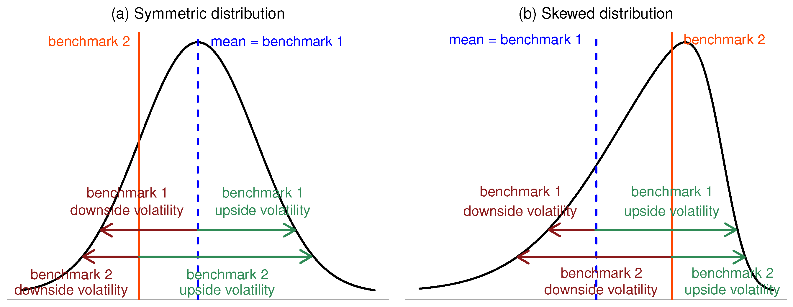
In short, if the returns are not symmetrically distributed or the benchmark is not equal to the mean, minimizing the standard deviation is not equivalent to minimizing the downside volatility, and targeting the variance is not in line with the investor’s preferences. Figure 1 illustrates the point.
When downside deviation is adopted as a measure of risk, the risk-adjusted return of the investment can be measured with the Sortino ratio (Sortino and Prince 1994):
where R is the average return of the investment.
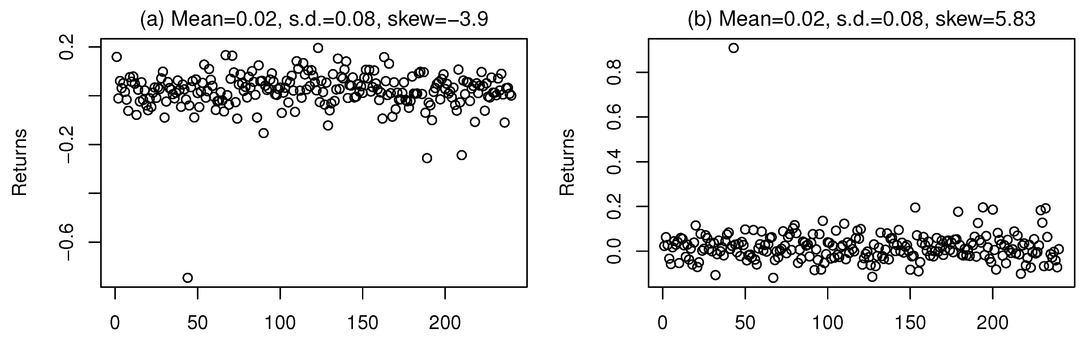
We show with a simple example why maximizing the Sortino ratio is preferable to maximizing the Sharpe ratio. Figure 2 shows two simulated series of returns with exactly the same mean (0.02) and standard deviation (0.08), but the one plotted on the left has a skew equal to −3.9, while the one plotted on the right has a skew equal to 5.83. While it is apparent that the latter, whose volatility is mostly due to high gains, is preferable to the former, whose volatility is driven by some catastrophic losses, in terms of the Sharpe ratio, the two series are exactly equivalent. However, the Sortino ratio tells a different story: with a benchmark , the Sortino ratio is equal to 0.242 for the negatively skewed series and to 0.491 for the positively skewed one. This is because the Sortino ratio is computed using the downside deviation, which accounts only for the volatility that actually hurts the investor.
3. The Semicovariance Matrix
In this section, we show what a semicovariance matrix is and we explain the endogeneity problem that afflicts it. We then present one of the solutions that have been proposed to solve it, which we will apply in this paper.
The semicovariance matrix is a covariance matrix computed by only considering the variability below a certain benchmark B.1 The diagonal elements of the semicovariance matrix are the semivariance terms, while the off-diagonal elements are the semicovariance terms. The semivariance of an asset’s returns is (Markowitz 1959)2
The semivariance of a portfolio of N assets (with returns ) and observation window T that underperforms the benchmark in K periods is defined in Markowitz (1959) as
where and are the weights of asset i and j, respectively. In accordance with Equation (4), the elements in the semicovariance matrix have to be computed in the same way one computes the terms of a covariance matrix, but only using the K periods in which the portfolio underperforms the benchmark B. The semicovariance matrix is therefore structured as follows:
where and are the semivariance and semicovariance terms, respectively. An alternative formula for the th element of is as follows:
where is an indicator function that takes value 1 if the return of the portfolio is lower than B, and 0 otherwise.
While Equation (3) does not pose any practical problem, following the logic of Equation (4) results in the estimation of an endogenous matrix; i.e., any change in the weights and changes the elements of . This happens because, with different weights, the portfolio underperforms the benchmark in different periods; therefore, the elements in are computed with a different K. This obviously makes Equation (4) unsuitable for procedures that compute optimal portfolio weights as output, since these same weights are needed to estimate an input (the semicovariance matrix) necessary for the optimization procedure. Even though a numerical solution of the problem is theoretically possible by discretizing the set of feasible portfolios and choosing the one with the lowest semivariance, implementing it is not feasible in practice unless the number of assets is extremely low.
3.1. Approximation of the Semicovariance Matrix
The endogeneity problem has been addressed by several scholars who propose different solutions, all of which have some drawbacks (see Estrada 2008, for a review). A heuristic approach that overcomes the problems of the previously existing solutions is devised in Estrada (2008), who proposes to use as input an approximation of computed as
instead of the exact estimation of the semicovariance matrix given by Equation (4). Equation (7) is based on whether individual assets, and not the portfolio as a whole, underperform B (as indicated by the letters in the suffix), and it yields the following exogenous and symmetric matrix:
can be used as input for portfolio optimization by simply substituting the covariance matrix with it (Estrada 2008). This replacement is all that is needed to turn mean-variance and minimum variance optimization procedures into mean-semivariance and minimum semivariance optimization procedures, respectively, allowing for an analytical solution of the problem. The closed-form solution to compute the optimal weights for the mean-variance portfolio is
where is the desired mean portfolio return, is the vector of mean returns, and is the covariance matrix. Therefore, using from now on to indicate the matrix in Equation (8) in order to simplify the notation, the mean-semivariance portfolio weights are simply given by
Analogously, since the minimum variance weights are
where is a vector of 1, the minimum semivariance weights are
3.2. Evaluating the Impact of the Approximation Error
In Estrada (2008), the author argues that the procedure he devised leads to a good approximation of the true semicovariance matrix, but he only supports his claim using a toy example. In Cheremushkin (2009), it is shown that, since the heuristic devised in Estrada (2008) does not account for upside returns of one asset that could compensate the downside returns of another asset, the approximation error can be large if the assets are negatively correlated, and still substantial for the uncorrelated case. The more the assets are positively correlated, the lower the error tends to be, disappearing when all the assets are perfectly positively correlated. One argument in favor of the heuristic in Estrada (2008) is that the correlation between financial assets is typically positive. Moreover, it is not clear how the approximation error actually impacts the efficiency of optimization procedures that use the heuristic in Estrada (2008) to estimate the downside risk input.
In order to quantify the loss caused by the approximation error in the semicovariance matrix, we consider 100 monthly stock return series from the CRSP dataset ranging from February 1973 to December 2016, and we select pairs of assets with different correlation coefficients . Only three pairs of stocks are negatively correlated to each other. The first pair of stocks we select is Exelon Corporation and Motorola Solutions, which have a correlation coefficient of , the most negative in the sample. The second pair is Southern Corporation and Navistar International Corporation, which are almost uncorrelated (). The third pair includes NextEra Energy and Altria Group, selected because their is equal to the average correlation coefficient of all the possible pairs of stocks in the dataset. Finally, the fourth pair is Schlumberg Limited and Halliburton Company, which with is the most positively correlated pair of stocks in the dataset. We then compute the sample mean and covariance matrix of each of these pairs of stocks and use them as inputs to generate series of 100,000 returns from a multivariate skew normal (see Azzalini and Dalla Valle 1996). For each pair, we set the individual skewness of both assets first equal to 0.3 and then to −0.3, to check for possible effects of the sign of the skewness on the results. We use the simulated series to compute the minimum semivariance weights using Equation (12), and we compare the downside deviation achieved out-of-sample with the one achieved by solving the problem numerically. To do so, we discretize the set of achievable portfolios by considering a grid of 1001 weights that span from 0 to 1 for each of the two risky assets. We then use Equation (4) to compute the semivariance of the portfolios obtained with each of the possible combinations, and select the one that has the lowest .
The inputs are estimated using a rolling window of 240 periods, and the benchmark B is set equal to a hypothetical risk-free rate of 0.1% per month. Table 1 shows the downside deviation achieved by the two strategies. Even with a negative correlation, the increase in downside deviation caused by the approximation error is only 2.2% when the skew is negative, and 4.5% when it is positive. With uncorrelated assets, the increase is of 3.9% and 8.2% with a negative and positive skew, respectively. With and , the increase is less then 1%. We now repeat the same exercise for the mean-semivariance portfolio. The numerical solution involves identifying the sets of weights that achieve the target excess return (which we set at 0.5% per period) and then selecting the one among these that has the lowest variance.3 The Sortino ratios achieved in this way and by applying the strategy in Estrada (2008) are shown in Table 2. With negatively correlated assets, the Sortino ratio achieved by applying the strategy in Estrada (2008) is significantly lower (10.4% and 14.8% with a negative and positive skew, respectively) than that achieved with a numerical solution. With the uncorrelated assets, the loss amounts to 2% with a negative skew and 5% with a positive skew. With , the loss is about 4.7% when the skew is negative and 5.5% when it is positive. Finally, with , the achieved Sortino ratio is 3.1% lower with the negative skew and 2.4% lower with the positive skew.
We can see that the impact of the approximation error does not decrease monotonically while approaching a perfect positive correlation. This is not surprising. Ceteris paribus, the approximation error decreases as the value of approaches 1. However, as pointed out in Cheremushkin (2009), the specific data used and the selected portfolio weights also have an impact. The effect of an increase in the correlation can be offset by these other factors, resulting in a higher error. More interesting is the fact that the impact of the approximation error is higher when computing the mean-semivariance portfolio than when the investor only minimizes the semivariance. Overall, the argument in Cheremushkin (2009) appears to have some practical relevance, especially when maximizing the Sortino ratio. Therefore, we decide to use the Estrada (2008) heuristic to estimate the semicovariance matrix in this paper, but in the analysis that we carry out in Section 4, we also look at the results obtained numerically.
3.3. Parameter Uncertainty in the Covariance and Semicovariance Matrix
With the endogeneity problem solved at the price of some performance loss, the solution in Estrada (2008) allows the mean-semivariance investor to achieve, in-sample, a higher (downside) risk-adjusted portfolio return than that obtained with mean-variance optimization, as Estrada (2008) shows. However, there is an additional issue not considered in Estrada (2008) that plays a crucial role when results are evaluated out-of-sample. The semicovariance matrix is computed, by definition, using only a subset of the available data, that is, only the returns that fall below the chosen benchmark B. Even if the exact sample semicovariance matrix could be computed with a zero approximation error, the estimate computed on T past periods would be less precise than the sample covariance matrix computed on the same T periods, because the actual estimation window would be smaller. Moreover, shrinkage estimators exist and are routinely used for estimating the covariance matrix, e.g., the one introduced in Ledoit and Wolf (2004). This estimator is a weighted average of (a) the sample covariance matrix and (b) a diagonal matrix with the same variance for all assets. The result is an estimator that is, asymptotically, both well-conditioned and more accurate than the sample covariance matrix. No equivalent solutions exist for the estimation of the semicovariance matrix. This makes it even harder for the semicovariance matrix to perform well out-of-sample compared to the covariance matrix.
In principle, if the data are skewed enough, the bias caused by assuming a symmetric distribution and using variance to measure risk should outweigh the negative impact of the higher parameter uncertainty. Analogously, given a certain non-zero skew, if the number of periods T is sufficiently high, the estimation error will be small enough for the bias to play a predominant role. However, how skewed or how long does the return series need to be in order for this to happen? In other words, does mean-semivariance optimization ever work well in realistic conditions? In the next section, we provide answers to this question.
4. Performance Comparison
We test the out-of-sample performance of the traditional and downside risk-based approaches in two different settings. In the first one, we consider only one asset and assess the accuracy of the estimated semivariance of the asset’s excess returns computed with and without the assumption of a symmetric distribution. In the second setting, we consider an asset menu with two risky assets and one risk-less asset, and compare the performances achieved by the mean-variance and minimum variance portfolios with those achieved by the mean-semivariance and minimum semivariance portfolios.
4.1. One Asset Case
When considering just one asset, the only parameter that needs to be estimated is the semivariance of the returns. We consider two possible estimators:
- The sample semivariance, given by Equation (3). This estimator is always unbiased but has a high variance for the reasons discussed in Section 3.3.
- , where is the sample variance. This estimator is biased, even asymptotically, unless the return distribution is perfectly symmetric, but it has a lower estimation error (i.e., a lower estimator variance).
The best estimator is the one with the lowest Mean Squared Error (MSE):
where .
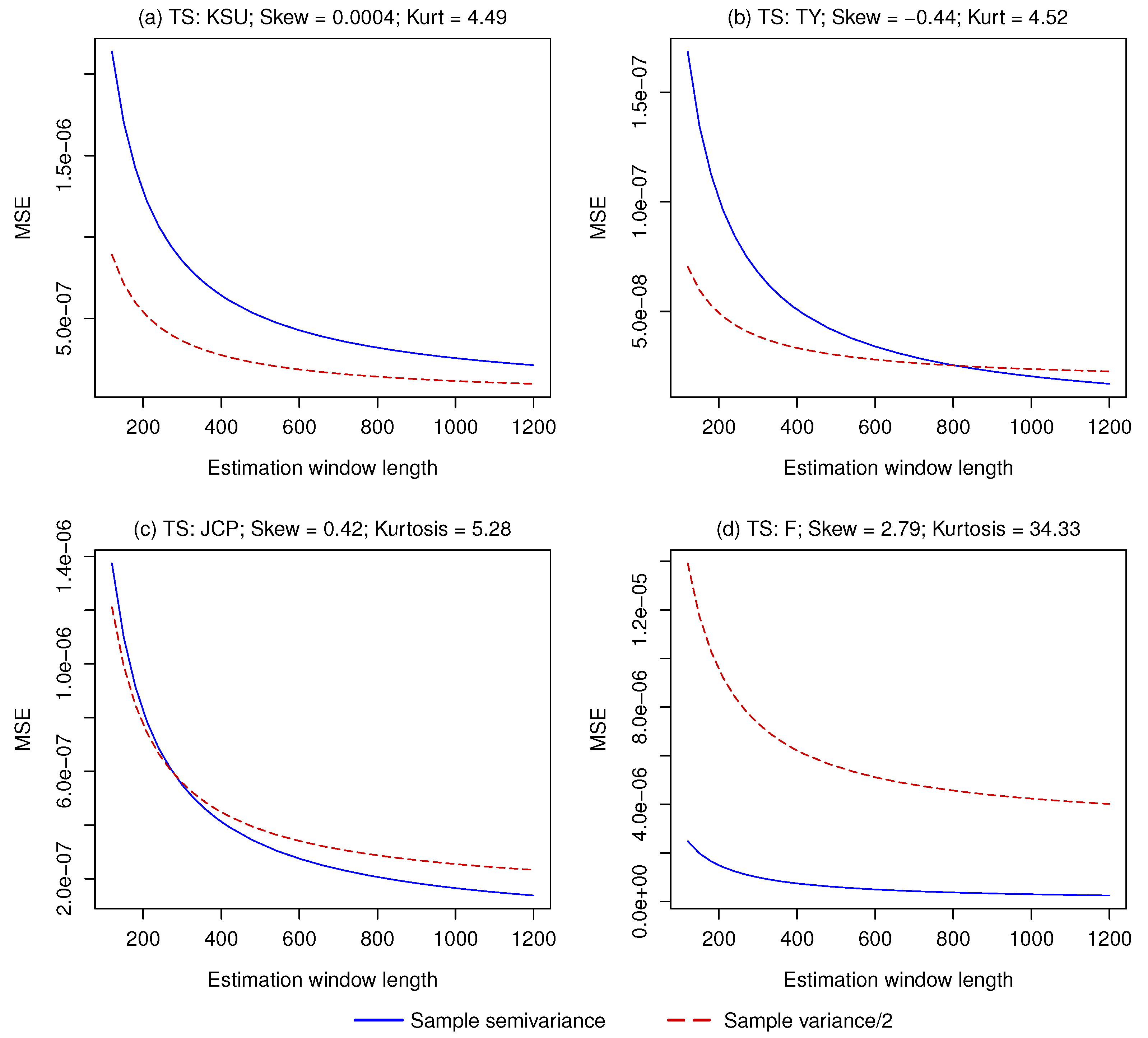
The relative importance of the two terms on the right side of Equation (13) depends on the shape of the distribution and on the number of periods used for estimation. The more asymmetric the distribution, the higher the bias of the second estimator is. The longer the estimation window, the lower the variance of both estimators is. In order to test empirically the performance of the two estimators, we generate series of 500,000 returns by drawing with replacement from the historical monthly returns, ranging from February 1973 to December 2016, of four stocks with different skewness from the CRSP dataset: Kansas City Southern, Tri-Continental Corporation, J. C. Penney, and Ford. In this way, we obtain series with approximately zero (Kansas City Southern), negative (Tri-Continental Corporation), positive (J. C. Penney), and very positive (Ford) skew, of which we know the exact semivariance. For each series, we set the benchmark B equal to the respective mean, we estimate the semivariance with both estimators using different estimation windows, and we compare the MSE. Figure 3 illustrates the results.
Unsurprisingly, when the return distribution is approximately symmetric, the lowest MSE is obtained by estimating the semivariance as half of the sample variance. When the skewness is equal to −0.44, the sample semivariance only has a lower MSE with an estimation window of about 800 periods or more. With a skew equal to 0.42, the sample semivariance becomes competitive with just 300 periods. Finally, with a very positive skew of 2.79, the MSE of the sample semivariance is always lower than that of the sample variance divided by 2.
4.2. Two Risky Assets Setting
We now consider the case of an investor who wants to allocate his wealth between two risky assets and one risk-free asset, and can choose between mean-variance and mean-semivariance portfolio optimization, which require the estimation of a covariance and semicovariance matrix, respectively. The performance measures that we use in this setting are those in line with the objective function of an investor with mean-semivariance preferences, i.e., the downside deviation and the Sortino ratio. Analogously to the case with one asset, using the semivariance should work best if, for a given T, the returns are sufficiently skewed, or, given a non-zero skew, T is sufficiently high. In addition to the portfolios computed using the sample covariance matrix and the semicovariance matrix approximated as in Estrada (2008), we also consider the one computed with the shrinkage estimation of the covariance matrix proposed in Ledoit and Wolf (2004). Finally, we solve numerically the semivariance-based optimization problem to evaluate the impact of the approximation error.
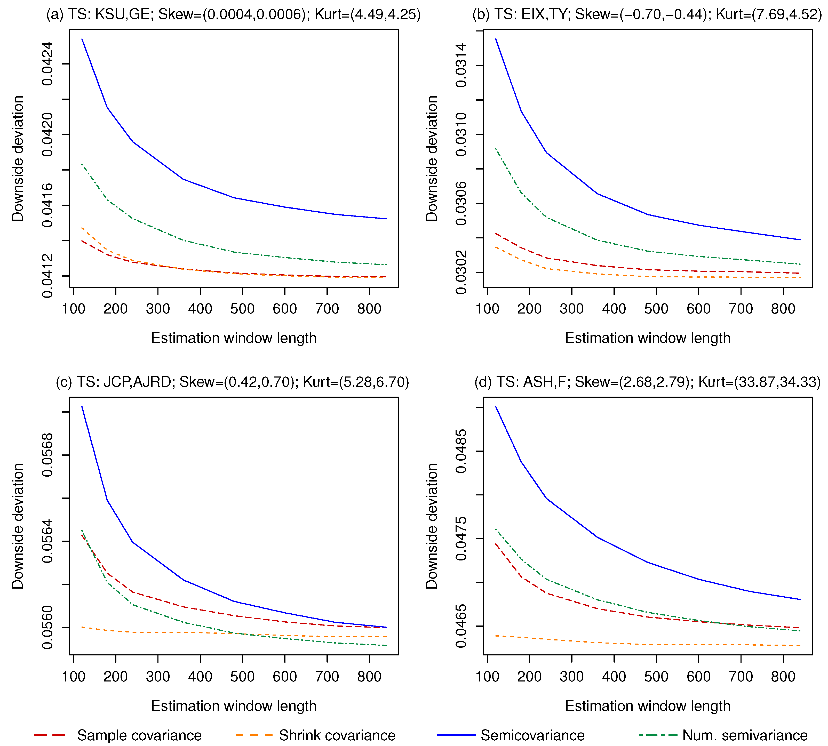
First, we test the ability of the different strategies to minimize the downside deviation. Therefore, we do not consider the mean, and we compute the minimum variance and minimum semivariance portfolios, using the inputs described above. We apply the strategies on series of 500,000 returns generated by drawing with replacement from monthly returns provided by the CRSP dataset, using pairs of stocks with virtually zero (Kansas City Southern and General Electric), negative (Edison International and Tri-continental Corporation), positive (J. C. Penney and Aerojet Rocketdyne Holdings Inc), and very positive (Ashland and Ford) skewness. We set the benchmark B equal to the risk-free rate, which is obtained from the Fama-French factors and drawn with replacement together with the risky assets’ returns.4 We compute the four portfolios using rolling windows of 120, 180, 240, and then up to 840 periods with steps of 120, and compute the downside deviation out-of-sample. Figure 4 shows the results.
As expected, when the asset returns show (almost) no skewness, the lowest portfolio semivariance can be achieved by minimizing the portfolio variance, with almost no performance difference between the sample and shrinkage estimate of the covariance matrix. Computing the minimum semivariance portfolio numerically works better than the Estrada (2008) solution, but not enough to catch up with the minimum variance portfolios. The same results hold for the portfolios constructed using assets with negatively skewed returns. The relative performance of the minimum semivariance portfolio improves when the returns are positively skewed, but only the numerically optimized one achieves the lowest semivariance, and only when more than 480 periods are used for the estimation. The situation changes again with the two strongly positively skewed assets, as even the numerical minimum semivariance portfolio never beats the minimum variance portfolio computed using the shrinkage estimate of the covariance matrix. A possible explanation is that a high kurtosis (observed in the returns of the two risky assets) negatively impacts the estimation of the semicovariance matrix more than the estimation of the covariance matrix. Since high skewness and high kurtosis are typically found together (in the 100 stock dataset considered here, the correlation between return skewness and kurtosis is 0.891), this result suggests that, in empirical series, after a certain point, a higher skewness does not make semivariance optimization more attractive. In all the four cases considered, the performance loss caused by the approximation error of the Estrada (2008) solution is non-negligible, but even the numerically optimized minimum semivariance portfolio is never the best choice.
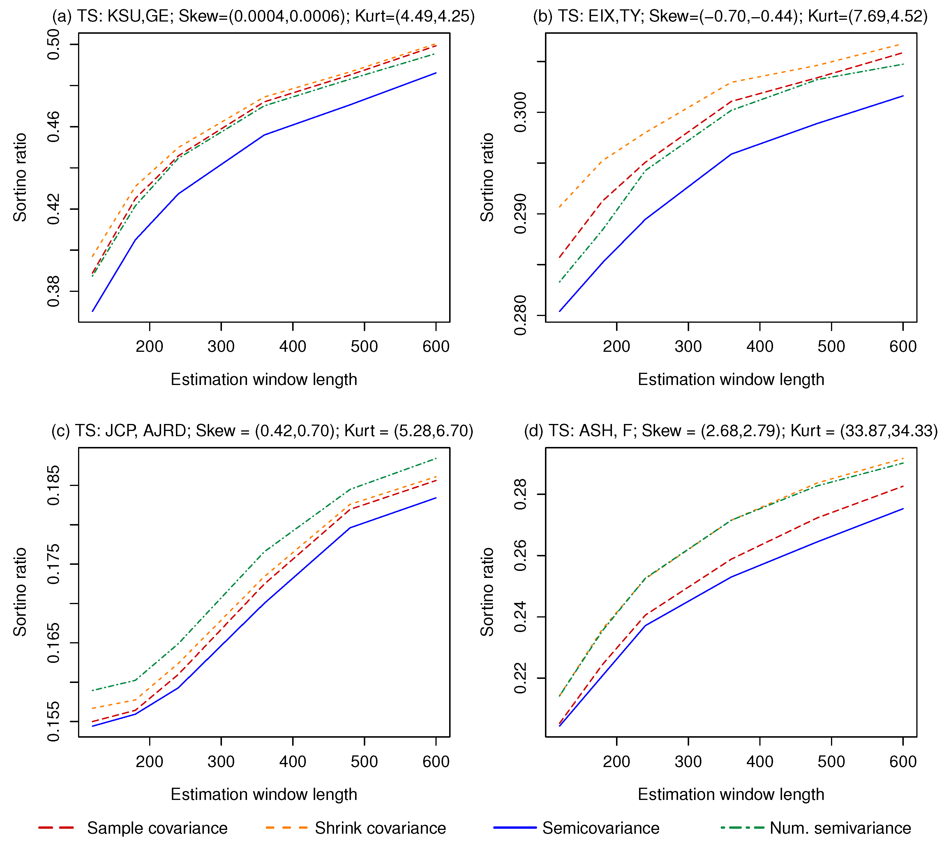
We now compute the mean-variance and mean-semivariance portfolios using the same series of returns. We exclude from the out-of-sample periods those periods in which the sum of the absolute value of the estimated of the two risky assets is lower than the desired portfolio excess return, which we set equal to 0.5%. This is done to avoid (extreme) allocations that require to invest more than 100% of the wealth only to achieve the required return (an inconvenience caused by having only two risky assets in order to make the numerical optimization feasible). On average, 5.3% of the out-of-sample periods are excluded for this reason. We evaluate each portfolio in terms of the Sortino ratio, computed with the same benchmark B used for estimating the semicovariance matrix. As with the minimum variance/semivariance portfolios, we set B equal to the risk-free rate.5 Figure 5 shows the results.
With non-skewed assets, the mean-semivariance portfolio considerably underperforms the other strategies when using the Estrada (2008) approximation, while the numerical optimization achieves a Sortino ratio very close to that of the mean-variance strategy. With a negative skew, using the approximated semicovariance matrix again gives the worst results, and the highest Sortino ratio is achieved by the mean-variance portfolio computed with the shrunk covariance matrix. With a positive skew, the mean-semivariance portfolio computed numerically works best, but using Estrada (2008), which is necessary in real situations with many assets, again gives the worst results. Finally, with a high positive skew, the shrunk covariance matrix and the numerical mean-semivariance optimization achieve a very similar Sortino ratio and are the best strategies, followed by the mean-variance portfolio computed with the sample covariance and finally by the mean-semivariance computed using Estrada (2008). For all the four pairs of stocks considered, the performance rank of the four strategies remains mostly stable across different estimation windows.
The first main conclusion we can draw from these results is that the approximation error in the semicovariance matrix computed as in Estrada (2008) causes a substantial performance loss. The second conclusion is that even the numerical solution (an approach that, in any case, is not feasible unless the number of assets is extremely low) is not competitive compared to the mean-variance optimization performed using the covariance matrix shrunk as in Ledoit and Wolf (2004), except when the asset returns are positively skewed (and show low kurtosis). Finally, in our experiment, a high kurtosis seems to hinder the effectiveness of mean-semivariance optimization more than it does with mean-variance optimization.
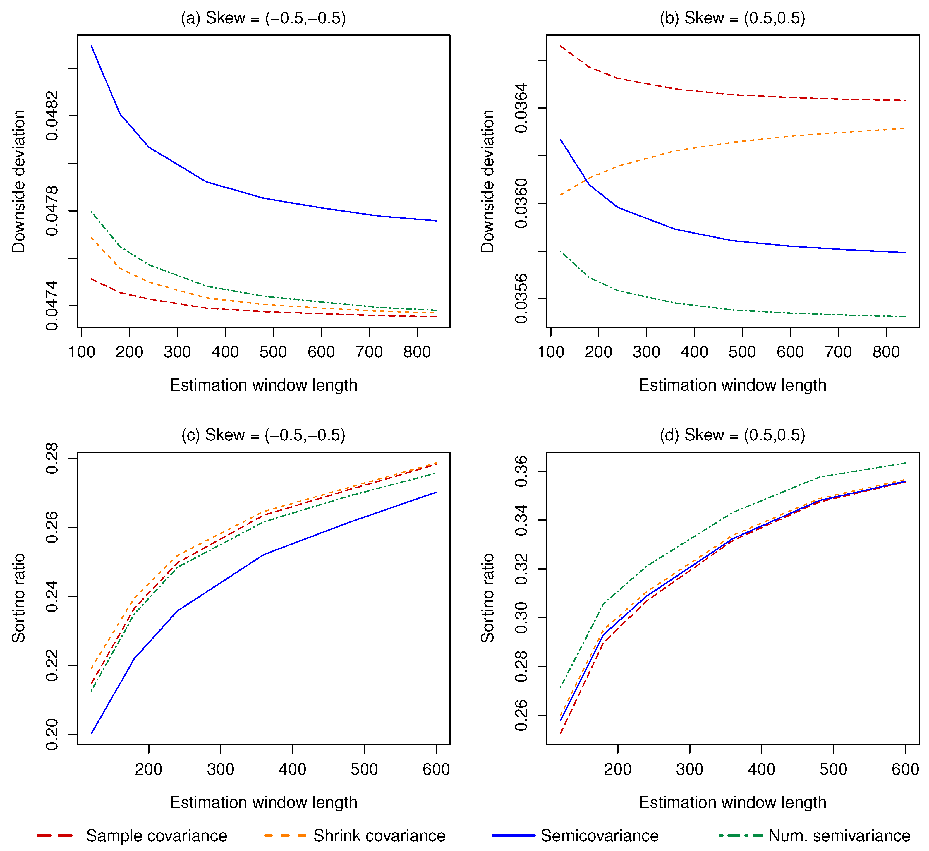
The different results observed with a negative and a positive skewness (and a similar kurtosis) deserve a deeper analysis. Intuitively, better results can be achieved when the skew is positive because, given a certain mean and variance, more observations fall below the benchmark and are therefore used in the estimation compared to when the skew is negative. To test this explanation, we repeat the computation of the minimum variance/semivariance and mean-variance/semivariance portfolios on 500,000 returns of two risky assets generated from a multivariate skew normal. We set the mean and covariance matrix equal to the sample estimates computed for Kansas City Southern and General Electric, and the skewness of both assets equal to −0.5 in one case and to 0.5 in the other. In this way, we isolate the effect of a different skewness on the results. The asset menu also includes one risk-less asset, whose return we set to 0.1% in every period, which is also the chosen value for the benchmark B. As expected, more individual asset returns fall below B when the skewness is positive (47.46% and 50.26% for the first and second asset, respectively) compared to when the skewness is negative (40.27% and 42.89%, respectively). The results of the portfolio optimization procedures, shown in Figure 6, are in line with those in Figure 4 and Figure 5. Overall, these results support the hypothesis that a positive skew allows for better results because the bulk of the data is located at the left of the distribution. This translates into more observations falling below B, and therefore a larger sample used for the estimation. The opposite happens when the skewness is negative.
5. Empirical Test of the Minimum Semivariance and Minimum CVaR Portfolios
Semivariance is definitely not the only measure that can be used by an investor who wants to minimize the downside risk. The CVaR, also known as Expected Shortfall, is a more popular alternative, and using it spares the investor from the efficiency loss caused by the approximation error of the Estrada (2008) solution. CVaR is based on the Value at Risk (VaR), which measures the maximum potential loss that can be suffered over a certain period, with a certain confidence level. CVaR, instead, measures the expected return of the portfolio given that the loss exceeds the VaR, and is generally regarded as a preferable measure of risk (see, e.g., Sarykalin et al. 2008; Yamai and Yoshiba 2002, for a description and comparison of the VaR and CVaR). However, in Lim et al. (2011), the authors claim that, while CVaR has many attractive theoretical properties, it is hard to actually profit from its practical application in risk management because of estimation difficulties. In fact, an investor that uses CVaR needs to correctly identify the tail behavior of the distribution, which is very difficult to do. In short, CVaR suffers from the same problem that afflicts the semicovariance matrix: The error in the estimation may be so great that minimizing the variance might be preferable, even if it is a less suitable risk measure from a theoretical point of view.
As a final test to assess the out-of-sample performance of downside risk optimization compared to the traditional variance-based approach, we carry out an empirical application that includes the minimum variance, minimum semivariance, and minimum CVaR portfolios. We choose to only minimize risk instead of computing mean-variance, mean-semivariance, and mean-CVaR portfolios for two reasons. First of all, we want to focus on the impact of using a specific risk measure, and including the estimated mean in the asset allocation decisions could drive most of the results, making it more difficult to assess the role of the chosen risk measure. Secondly, as argued in Jagannathan and Ma (2003), the sample mean is such an imprecise estimate of the true mean that ignoring it yields portfolios with a higher Sharpe ratio. We also consider the minimum variance, minimum semivariance, and minimum CVaR portfolios with the additional constraint of no short selling allowed, which, as shown in Jagannathan and Ma (2003), considerably improves out-of-sample performance when minimizing risk. Finally, we include as benchmark the naïve 1/N rule. The estimation of the covariance matrix for the minimum variance portfolio is carried out using the shrinkage technique introduced in Ledoit and Wolf (2004). For the computation of the minimum CVaR portfolio, we resort to the formulation proposed in Rockafellar and Uryasev (2000). We do not assume any specific distribution for the returns, and rely instead on the historical distribution. The confidence interval is set to 95%.
An additional goal of this application on real empirical data is to evaluate the performance of the semivariance-based optimization without the limitations posed by the analysis on the simulated data considered in Section 4. While the return series used were data-driven (since they were generated by sampling from empirical series), the framework is still not equivalent to the setting in which a real investor operates. The first reason is that data generated by sampling with replacement are homoskedastic, while real financial return series show heteroskedasticity. Moreover, in sampled data, the true values of and remain the same throughout the series, while in empirical data the true value of the parameters change through time. This means that, while with sampled data a longer estimation window always translates into better estimates, with empirical series, using data that are too distant in the past can be inappropriate, since they contain outdated information. Another aspect not evaluated in Section 4 is the impact of the coskewness terms, which can be even more important than idiosyncratic skewness terms (Albuquerque 2012). Finally, in order to make it feasible to numerically compute the minimum semivariance and mean-semivariance portfolios, the analysis was restricted to portfolios with only two risky assets.
For this empirical application, we use weekly returns from 23 February 1990, to 1 April 2016, provided in Bruni et al. (2016) for 28 of the 30 stocks that make up the Dow Jones Industrial Average.6 We choose weekly returns because they allow for a large number of out-of-sample periods without requiring many decades of data, which are often not available for individual stocks. We test two different rolling windows of 5 and 10 years, obtaining 843 out-of-sample returns. We set B equal to the risk free rate, which we get from the Fama-French factors dataset. Results are reported in Table 3 and Table 4. “Min Var,” “Min Semivar,” and “Min CVaR” indicate the minimum variance, minimum semivariance, and minimum CVaR portfolios, respectively, while “Long” indicates that the given strategy is implemented with a long-only constraint.
With a 5 year rolling window, the lowest downside deviation (and, as expected, the lowest standard deviation) is achieved by the two minimum variance portfolios, followed closely by the minimum semivariance portfolio without short positions. The 1/N rule achieves the highest Sortino ratio, followed by the minimum variance with no short selling; all the other strategies lay far behind. The best result in terms on CVaR is obtained by minimizing the variance; the second-best result is obtained by minimizing the semivariance without short selling; the third-best result is obtained by minimizing the semivariance; only in fourth position do we have the minimum CVaR portfolio without short selling. Overall results improve with a 10 year rolling window (except, of course, for the naïve one), but the relative performance of the different portfolios remain very similar. Minimizing the variance is again the best choice for an investor that wants to minimize the downside deviation. The best Sortino ratio is achieved by the minimum variance portfolio without short selling, followed closely by the 1/N rule. The minimum CVaR portfolio considerably improves its performance, but only ranks third, behind the two minimum variance portfolios. Overall, results in Table 3 and Table 4 confirm what found in Section 4, and are in line with Lim et al. (2011).
6. Conclusions
When setting an objective function for asset allocation decisions, an investor has to consider not only how well it represents his preferences, but also how difficult it is to efficiently apply it in practice. We showed empirically that this trade-off provides a rational motivation for the popularity of variance as a measure of risk. Minimizing the semivariance is more in line with the true preferences of a rational investor, but minimizing the variance usually achieves a lower downside deviation and a higher Sortino ratio because it can be estimated more accurately. Analogous results were observed in an empirical application in which CVaR is used as an alternative measure of downside risk. In fact, the message of this paper is that the problem lies not in a specific measure of downside risk, but in the concept of downside risk. Minimizing only the losses instead of all variability may be perfectly reasonable from a theoretical point of view, but it requires the investor to estimate the necessary inputs using only a fraction of the available information. This translates into imprecise estimates, which lead to poor out-of-sample portfolio performance. The traditional variance-based optimization is therefore preferable in most cases even for an investor with downside risk preferences.
Funding
This research received no external funding.
Acknowledgments
I would like to thank Alex Weissensteiner for his invaluable suggestions and help for this work.
Conflicts of Interest
The author declares that there is no conflict of interest.
References
- Albuquerque, Rui. 2012. Skewness in stock returns: Reconciling the evidence on firm versus aggregate returns. The Review of Financial Studies 25: 1630–73. [Google Scholar] [CrossRef]
- Azzalini, Adelchi, and Alessandra Dalla Valle. 1996. The multivariate skew-normal distribution. Biometrika 83: 715–26. [Google Scholar] [CrossRef]
- Bruni, Renato, Francesco Cesarone, Andrea Scozzari, and Fabio Tardella. 2016. Real-world datasets for portfolio selection and solutions of some stochastic dominance portfolio models. Data in Brief 8: 858–62. [Google Scholar] [CrossRef] [PubMed]
- Cheremushkin, Sergei V. 2009. Why D-CAPM is a big mistake? The incorrectness of the cosemivariance statistics. SSRN Electronic Journal. [Google Scholar] [CrossRef]
- Estrada, Javier. 2008. Mean-semivariance optimization: A heuristic approach. Journal of Applied Finance 18: 57–72. [Google Scholar] [CrossRef] [Green Version]
- Jagannathan, Ravi, and Tongshu Ma. 2003. Risk reduction in large portfolios: Why imposing the wrong constraints helps. The Journal of Finance 58: 1651–84. [Google Scholar] [CrossRef] [Green Version]
- Ledoit, Olivier, and Michael Wolf. 2004. A well-conditioned estimator for large-dimensional covariance matrices. Journal of Multivariate Analysis 88: 365–411. [Google Scholar] [CrossRef] [Green Version]
- Lim, Andrew E.B., J. George Shanthikumar, and Gah-Yi Vahn. 2011. Conditional value-at-risk in portfolio optimization: Coherent but fragile. Operations Research Letters 39: 163–71. [Google Scholar] [CrossRef]
- Markowitz, Harry. 1952. Portfolio selection. The Journal of Finance 7: 77–91. [Google Scholar]
- Markowitz, Harry. 1959. Portfolio Selection. New York: John Wiley and Sons. [Google Scholar]
- Rockafellar, Ralph T., and Stanislav Uryasev. 2000. Optimization of Conditional Value-at-Risk. Journal of Risk 2: 21–41. [Google Scholar] [CrossRef] [Green Version]
- Sarykalin, Sergey, Gaia Serraino, and Stan Uryasev. 2008. Value-at-Risk vs. Conditional Value-at-Risk in risk management and optimization. In State-of-the-Art Decision-Making Tools in the Information-Intensive Age. INFORMS Tutorials in Operations Research. Catonsville: INFORMS, pp. 270–94. [Google Scholar]
- Sortino, Frank A., and Lee N. Prince. 1994. Performance measurement in a downside risk framework. The Journal of Investing 3: 59–64. [Google Scholar] [CrossRef]
- Yamai, Yasuhiro, and Toshinao Yoshiba. 2002. On the validity of Value-at-Risk: Comparative analyses with expected shortfall. Monetary and Economic Studies 20: 57–85. [Google Scholar]
| 1. | Formally, this is the lower semicovariance matrix. The upper semicovariance matrix, which measures variability only above the benchmark, can also be computed. Since we are only interested in the former, throughout the paper we refer to it simply as a “semicovariance matrix”. |
| 2. | Notice that the semivariance is simply the square of the downside deviation, defined in Equation (1). |
| 3. | While it is possible to identify sets of weights that perfectly match the target expected return, for computational reasons, we consider the combinations with an expected portfolio return between 0.4995% and 0.5005% |
| 4. | We deem it preferable to base the risk-free rate on real data when possible, as it is when we generate series by drawing with replacement from empirical series of returns. We only use an arbitrary risk-free rate equal to 0.1% when simulating by drawing from a multivariate skew normal, as we did in Section 3.2. |
| 5. | Setting B equal to the target return is also reasonable, but if the out-of-sample portfolio return is lower than the target, this would lead to a negative Sortino ratio, which would make it difficult to interpret the results. Moreover, using the same B used when minimizing the volatility improves the comparability of the results. |
| 6. | We change the data source from the CRSP database to the dataset from Bruni et al. (2016) for reasons of data availability, as we do not have access to weekly returns from CRSP. |
Figure 1.
(a) With a symmetric distribution and a benchmark equal to the mean, downside and upside volatility are equally split; (b) With a skewed distribution or a benchmark different from the mean, downside and upside volatility are uneven.
Figure 1.
(a) With a symmetric distribution and a benchmark equal to the mean, downside and upside volatility are equally split; (b) With a skewed distribution or a benchmark different from the mean, downside and upside volatility are uneven.

Figure 2.
Two very different series with the same mean and standard deviation. (a) Negatively skewed series; (b) Positively skewed series.
Figure 2.
Two very different series with the same mean and standard deviation. (a) Negatively skewed series; (b) Positively skewed series.

Figure 3.
Mean Squared Error of the sample semivariance and the sample variance/2 used as estimators for the semivariance of a series of returns. (a) Virtually symmetrically distributed returns; (b) Negatively skewed returns; (c) Positively skewed returns; (d) Very positively skewed returns.
Figure 3.
Mean Squared Error of the sample semivariance and the sample variance/2 used as estimators for the semivariance of a series of returns. (a) Virtually symmetrically distributed returns; (b) Negatively skewed returns; (c) Positively skewed returns; (d) Very positively skewed returns.

Figure 4.
Downside deviation achieved by minimum variance/semivariance portfolios constructed with assets with different idiosyncratic skewness. (a) Virtually zero skew; (b) Negative skew; (c) Positive skew; (d) Very positive skew.
Figure 4.
Downside deviation achieved by minimum variance/semivariance portfolios constructed with assets with different idiosyncratic skewness. (a) Virtually zero skew; (b) Negative skew; (c) Positive skew; (d) Very positive skew.

Figure 5.
Sortino ratio achieved by mean-variance/semivariance portfolios constructed with assets with different idiosyncratic skewness. (a) Virtually zero skew; (b) Negative skew; (c) Positive skew; (d) Very positive skew.
Figure 5.
Sortino ratio achieved by mean-variance/semivariance portfolios constructed with assets with different idiosyncratic skewness. (a) Virtually zero skew; (b) Negative skew; (c) Positive skew; (d) Very positive skew.

Figure 6.
Portfolio performance with asset returns generated from a multivariate skew normal distribution. (a) Minimum variance/semivariance portfolios with negatively skewed asset returns; (b) Minimum variance/semivariance portfolios with positively skewed asset returns; (c) Mean-variance/semivariance portfolios with negatively skewed asset returns; (d) Mean-variance/semivariance portfolios with positively skewed asset returns.


Table 1.
Downside deviation of minimum semivariance portfolios with multivariate skew normal returns and 240 months rolling windows. Benchmark = risk-free rate (0.1%).
Table 1.
Downside deviation of minimum semivariance portfolios with multivariate skew normal returns and 240 months rolling windows. Benchmark = risk-free rate (0.1%).
| Corr. | Skew | Estrada (2008) | Numerical |
|---|---|---|---|
| −0.013 | (−0.3, −0.3) | 0.0371 | 0.0363 |
| −0.013 | (0.3, 0.3) | 0.0280 | 0.0268 |
| 0.003 | (−0.3, −0.3) | 0.0323 | 0.0311 |
| 0.003 | (0.3, 0.3) | 0.0265 | 0.0245 |
| 0.300 | (−0.3, −0.3) | 0.0328 | 0.0326 |
| 0.300 | (0.3, 0.3) | 0.0263 | 0.0261 |
| 0.743 | (−0.3, −0.3) | 0.0566 | 0.0563 |
| 0.743 | (0.3, 0.3) | 0.0508 | 0.0506 |
Table 2.
Sortino ratio of mean-semivariance portfolios with multivariate skew normal returns and 240 months rolling windows. Benchmark = risk-free rate (0.1%).
Table 2.
Sortino ratio of mean-semivariance portfolios with multivariate skew normal returns and 240 months rolling windows. Benchmark = risk-free rate (0.1%).
| Corr. | Skew | Estrada (2008) | Numerical |
|---|---|---|---|
| −0.013 | (−0.3, −0.3) | 0.1894 | 0.2114 |
| −0.013 | (0.3, 0.3) | 0.2499 | 0.2932 |
| 0.003 | (−0.3, −0.3) | 0.2779 | 0.2837 |
| 0.003 | (0.3, 0.3) | 0.3202 | 0.3371 |
| 0.300 | (−0.3, −0.3) | 0.3391 | 0.3560 |
| 0.300 | (0.3, 0.3) | 0.4221 | 0.4467 |
| 0.743 | (−0.3, −0.3) | 0.1388 | 0.1433 |
| 0.743 | (0.3, 0.3) | 0.1445 | 0.1481 |
Table 3.
5 year rolling window estimation.
| Strategy | St.Dev. | Dw.Dev. | Sharpe | Sortino | CVaR |
|---|---|---|---|---|---|
| 1/N | 0.0254 | 0.0172 | 0.0535 | 0.0791 | −0.0555 |
| Min Var | 0.0193 | 0.0140 | 0.0399 | 0.0552 | −0.0449 |
| Min Var Long | 0.0197 | 0.0139 | 0.0504 | 0.0713 | −0.0454 |
| Min Semivar | 0.0223 | 0.0163 | 0.0011 | 0.0014 | −0.0521 |
| Min Semivar Long | 0.0204 | 0.0144 | 0.0344 | 0.0485 | −0.0459 |
| Min CVaR | 0.0225 | 0.0168 | 0.0035 | 0.0047 | −0.0539 |
| Min CVaR Long | 0.0206 | 0.0148 | 0.0280 | 0.0389 | −0.0484 |
Table 4.
10 year rolling window estimation.
| Strategy | St.Dev. | Dw.Dev. | Sharpe | Sortino | CVaR |
|---|---|---|---|---|---|
| 1/N | 0.0254 | 0.0172 | 0.0535 | 0.0791 | −0.0555 |
| Min Var | 0.0196 | 0.0138 | 0.0487 | 0.0689 | −0.0454 |
| Min Var Long | 0.0205 | 0.0141 | 0.0549 | 0.0795 | −0.0465 |
| Min Semivar | 0.0210 | 0.0150 | 0.0094 | 0.0132 | −0.0483 |
| Min Semivar Long | 0.0209 | 0.0145 | 0.0374 | 0.0537 | −0.0478 |
| Min CVaR | 0.0207 | 0.0148 | 0.0055 | 0.0077 | −0.0468 |
| Min CVaR Long | 0.0205 | 0.0143 | 0.0379 | 0.0546 | −0.0470 |
© 2020 by the author. Licensee MDPI, Basel, Switzerland. This article is an open access article distributed under the terms and conditions of the Creative Commons Attribution (CC BY) license (http://creativecommons.org/licenses/by/4.0/).
Share and Cite
MDPI and ACS Style
Rigamonti, A. Mean-Variance Optimization Is a Good Choice, But for Other Reasons than You Might Think. Risks 2020, 8, 29. https://doi.org/10.3390/risks8010029
AMA Style
Rigamonti A. Mean-Variance Optimization Is a Good Choice, But for Other Reasons than You Might Think. Risks. 2020; 8(1):29. https://doi.org/10.3390/risks8010029
Chicago/Turabian StyleRigamonti, Andrea. 2020. "Mean-Variance Optimization Is a Good Choice, But for Other Reasons than You Might Think" Risks 8, no. 1: 29. https://doi.org/10.3390/risks8010029
Note that from the first issue of 2016, this journal uses article numbers instead of page numbers. See further details here.