Hydraulic and Hydrologic Analysis of Unsteady Flow in Prismatic Open Channel †

School of Civil Engineering, National Technical University of Athens,9 Iroon Polytechniou St., 15780 Athens, Greece
*
Author to whom correspondence should be addressed.
†
Presented at the 3rd EWaS International Conference on “Insights on the Water-Energy-Food Nexus”, Lefkada Island, Greece, 27–30 June 2018.
Proceedings 2018, 2(11), 571; https://doi.org/10.3390/proceedings2110571
Published: 2 August 2018
(This article belongs to the Proceedings of EWaS3 2018)
Abstract
:Comparison between hydraulic and hydrologic computational methods is conducted in this study, regarding prismatic open channels under unsteady subcritical flow conditions. One-dimensional unsteady flow continuity and momentum equations are solved using explicit and implicit finite difference schemes for a symmetrical trapezoidal cross section, where the flow discharge and depth are the dependent variables. The results have been compared to those derived from Muskingum-Cunge hydraulic/hydrologic method as well as the commercial software HEC-RAS. The results from explicit and implicit code compare well to those from commercial software and hydraulic/hydrologic methods for long prismatic channels, thus directing the hydraulic engineer to quick preliminary design of prismatic open channels for unsteady flow with satisfactory accuracy.
1. Introduction
Different types of open channels such as prismatic canals or natural streams usually operate under unsteady flow conditions. Unsteady flow analysis for storm sewers as well as for natural streams is significant during a flood event. It is common practice that engineers usually compute the flow depth in a channel assuming steady flow at peak discharge for flood related studies. However, this approach is conservative, since it does not account for the attenuation of flood wave, resulting from wall friction and water storage in the channel. Using steady flow analysis one cannot determine the time the peak flow occurs at a location of interest along a watercourse. Accurate prediction of flood-wave propagation in open channels is only possible if the unsteady open channel flow equations are used. The unsteady flow computation in open channels is referred to as flood or channel routing.
The unsteady open channel Saint Venant equations of motion used for computations are the continuity equation written as:
and the momentum equation,
A = A(x, t) is the wetted cross-sectional area and Q = Q(x, t) the flow rate, both being functions of time t and the distance x from the upstream end of the channel in the main flow direction. V(x, t) is the average cross-sectional velocity, y(x, t) the flow depth, So the longitudinal channel slope, Sf = n2V|V|/R4/3 the friction slope derived from Manning’s formula accounting also for reverse flow conditions, n the Manning friction coefficient, g the gravitational acceleration, and β a correction factor related to the cross sectional time-averaged velocity distribution. The assumptions used to derive the equations of motion above include (1) the hydrostatic pressure distribution, (2) the uniform velocity over the channel section, (3) the small average channel bed slope, and (4) the homogeneous and incompressible flow. From these assumptions β = 1, and substitution of V = Q/A in Equation (2) yields:
Unsteady-flow equations are complex, and generally are not amenable to closed-form analytical solutions. Thus, numerical methods such as finite difference and finite element methods must be used to solve these equations. Many numerical methods are available for solving the complete dynamic-wave equations in their direct or characteristic form and their approximations in Cartesian coordinate system. Such methods can be broadly classified as explicit [1,2], and implicit [3,4,5,6,7,8,9], for solving the equations in their direct form. Also, the system of equations can be solved in a curvilinear coordinate system in case that the flow geometry is more complex [10,11,12,13,14].
From the hydrologic perspective, the Muskingum-Cunge method dated back in 1969 can be used for flood routing calculation. It is based on the storage equation (continuity equation) and considering the momentum equation it relates the storage S, the input and output flow rates I and Q respectively, with a linear relationship in a specific channel reach. The Muskingum–Cunge method, however, is based on the kinematic-wave approximation of the Saint Venant equations modified with diffusion contributions of the momentum equation, so it can represent the real behavior of flood wave propagation [15].
Objective of this work is to reveal the practical aspects of code implementation for the explicit as well as the implict Preissmann finite difference schemes, for the solution of the complete dynamic wave equations in a prismatic channel with symmetrical trapezoidal cross-section, under subcritical flow conditions. The computational results will be compared to those derived from the application of unsteady one dimensional HEC-RAS v. 4.1 software [16] and from the Muskingum-Cunge method.
2. Numerical Solution Methods—Explicit and Implicit Scheme
The Saint Venant equations are partial differential equations of hyperbolic type requiring one initial and two boundary conditions to be solved. The initial condition is a snap shot of the flow parameters Q and y, along the channel at time zero, which in the present work is steady flow with constant flowrate and flow depth derived from Manning formula. The flow is subcritical, therefore one boundary condition at each end of the channel is required.
The finite difference equations are obtained using truncated Taylor series approximation of the partial differential terms of the Saint Venant equations. This approximation causes truncation errors which are related to the discretization of space and time and the nature of the approximations used to convert the continuous equations to discrete ones. Error accumulation can potentially make the results of the numerical method invalid. A numerical method must be consistent, convergent, and stable to produce acceptable results i.e., consistent if the continuous governing equations are obtained from the finite difference equations as both the space increment Δx, and the time increment Δt, approach zero, convergent if Δx and Δt are reduced the results approach limiting values that match the true solution of the governing differential equations, and stable if round-off and truncation errors do not accumulate to make the solution diverge [15].
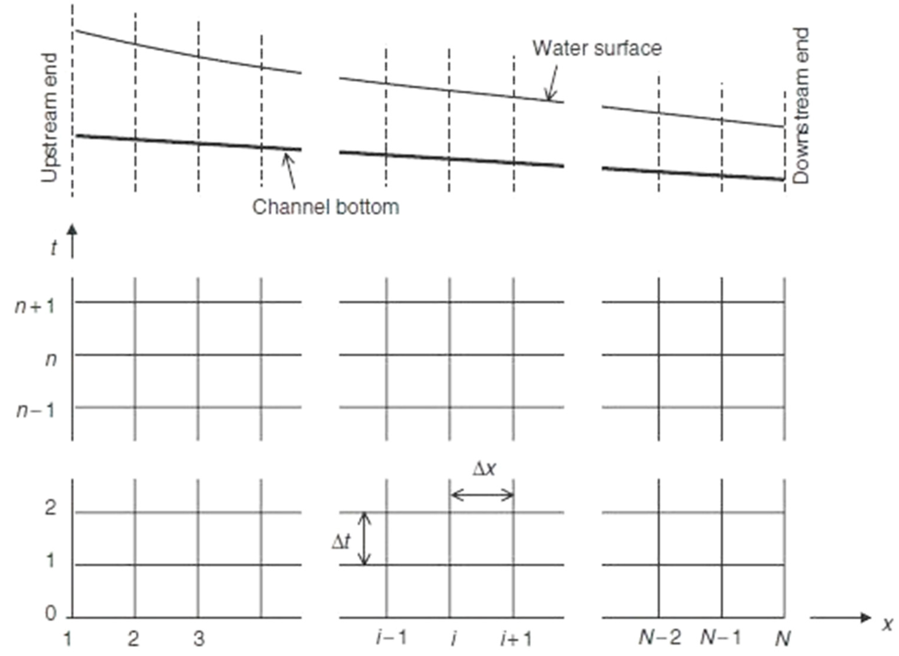
To apply the finite difference method, we discretize the channel length into N nodes, I = 1, 2, …, N, of N − 1 reaches as shown in the Figure 1, the time variable into n + 2 nodes, n = 0, 1, …, n + 1 and seek solutions only for these discrete time stages. The vertical lines of the computational grid represent different locations along a channel, and the horizontal lines correspond to the discrete times at which we seek the numerical solution. Both space and time increments Δx and Δt are constant. The horizontal line marked 0 represents the initial time (t = 0), and the flow conditions are known at all spatial nodes on this line from the initial conditions. The vertical line labeled as 1 represents the upstream end of the channel while that labeled N represents the downstream end. The boundary conditions apply to the nodes on these lines.
Regarding the explicit scheme, Equations (1) and (3) are the governing equations of the algorithm, so if we discretize all the spatial partial derivatives at time stage n with central differences by minimizing the truncation error of order O(Δx2) we can obtain an explicit algorithm for the calculation of , at time stage n + 1 from the known quantities , , either from the initial condition or from the calculations of the previous time step while altering the discretization of continuity equation at first and final boundary spatial node due to programming reasons. Concerning the implicit four-point scheme, the values at time stage n + 1 as well as stage n are used to approximate the spatial derivatives of the dependent variables of the Saint Venant equations. This formulation does not lead to explicit expressions to evaluate the variables at time stage n + 1, however a non-linear system of algebraic equations is obtained which is solved by Newton-Raphson methodology. These equations are solved simultaneously to obtain the results at time stage n + 1 all at once. Details can be found in [15]. The numerical codes have been implemented in house using Matlab® computational environment.
3. Hydraulic/Hydrologic Method
The Muskingum-Cunge method dated back in 1969, is based on the diffusive wave model of continuity and simplified momentum equation, keeping only gravity, friction and hydrostatic pressure terms [15]:
Combination of Equations (4) and (5) yields the one-dimensional Burgers equation of the unknown discharge, including unsteady, advection and diffusion terms, where C is the kinematic wave celerity and D the coefficient of hydraulic diffusivity:
Equation (6) is discretized and solved numerically using finite differences of constant time increment Δt. After some analysis we end up with Equation (7) for the calculation of the downstream hydrograph, which are the same with equations obtained using the classic hydrologic storage (continuity) equation dS/dt = I-Q, S being the volume of water stored in the channel reach, I is the inflow upstream and Q is the outflow downstream:
where the subscripts 1 and 2 correspond to time levels n and n + 1 respectively, , , Q0 is a reference discharge, T0 is the top width corresponding to the reference discharge, V0 is the cross-sectional average velocity corresponding to the reference discharge, S0 is the longitudinal slope of the channel, L is the length of the channel reach, and m = 5/3, [15]. The base flow rate, the peak of the inflow hydrograph, or the average inflow rate can be used as the reference discharge showing small sensitivity in the final results. It is also suggested that Δt must be smaller than one-fifth of the time from the beginning to the peak of the inflow hydrograph [15]. Moreover, it is recommended that the length of the channel reach for Muskingum–Cunge computations must be limited according to the following relationship [15]:
for better accuracy.
4. Results
4.1. Explicit Algorithm
In this section we present the results from the explicit algorithm, the HEC-RAS v. 4.1 software [17], and Muskingum-Cunge algorithm. More specifically the results regard a 9000 m long open channel of symmetrical trapezoidal cross section with 1H:1V side slope and 5 m bottom width, Manning coefficient 0.025 and longitudinal bottom slope of 0.001. The of flood wave time was 20,000 s (5.55 h). The initial condition was steady, uniform flow, with base flow rate of 2 m3/s whereas the upstream boundary condition was a known inflow hydrograph of the form:
Q(x = 0, t) = Qmin + (Qmax − Qmin)((t/tmax)1.5)exp(1.5(1 − (t/tmax)))
Q(t) is the variable flow rate at time t, Qmin = 2 m3/s is the base flow, Qmax = 200 m3/s is the maximum flood flow rate and tmax = 2000 s is the time at which peak of flow occurs representing as close as possible the flood hydrograph of a typical Greek stream. The downstream boundary condition applied was uniform flow at any time stage.
Implementing the code, for simplicity we used uniform temporal and spatial discretization with 15,000 and 300 nodes respectively for stability reasons. We have kept the same parameters for HEC-RAS calculations, whereas in Muskingum-Cunge calculations the reference discharge was selected to be one half of the peak discharge with time step of 60 s. The maximum percentage error of mass conservation at the resulting downstream hydrographs was 0.52%.
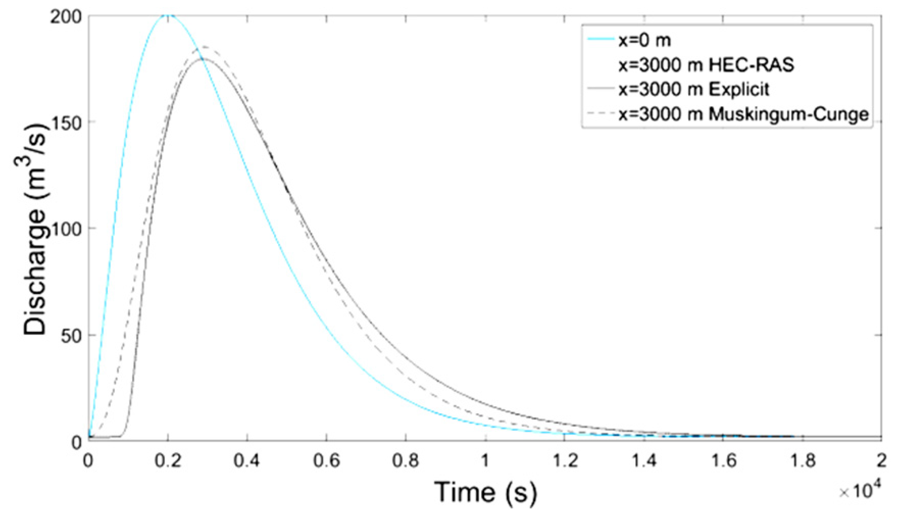
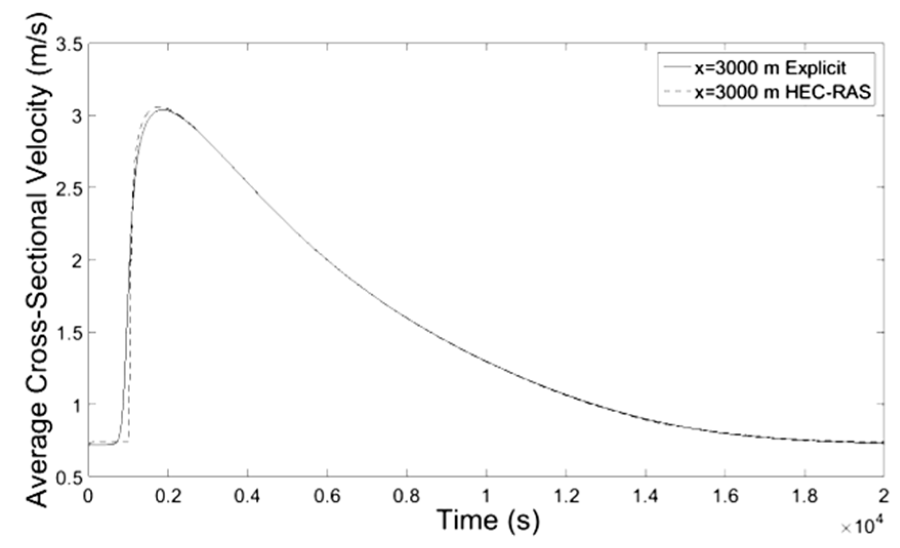
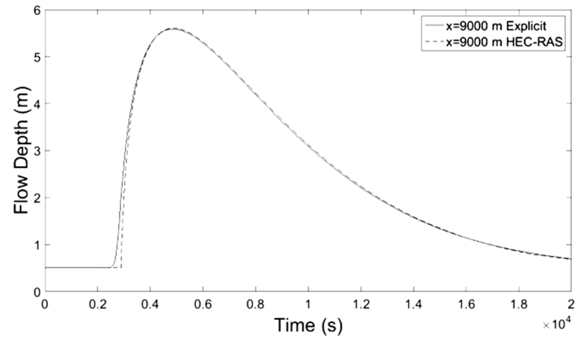
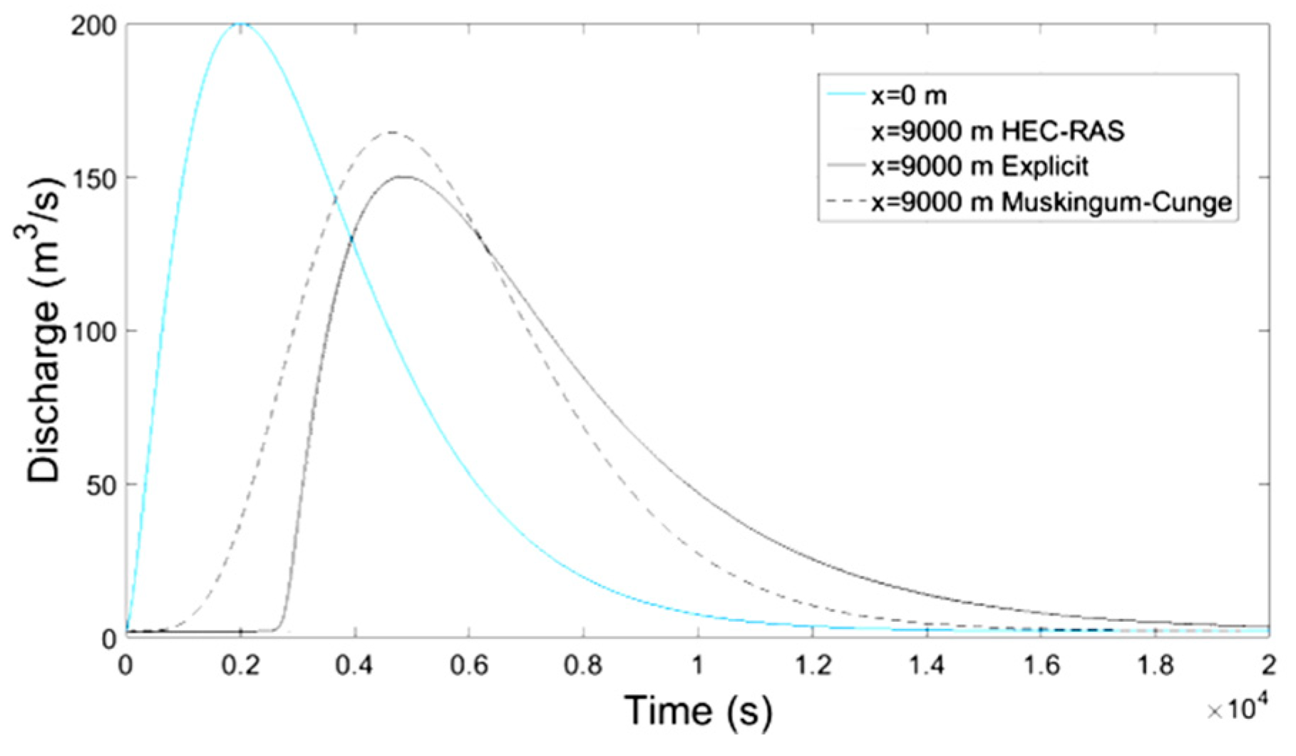
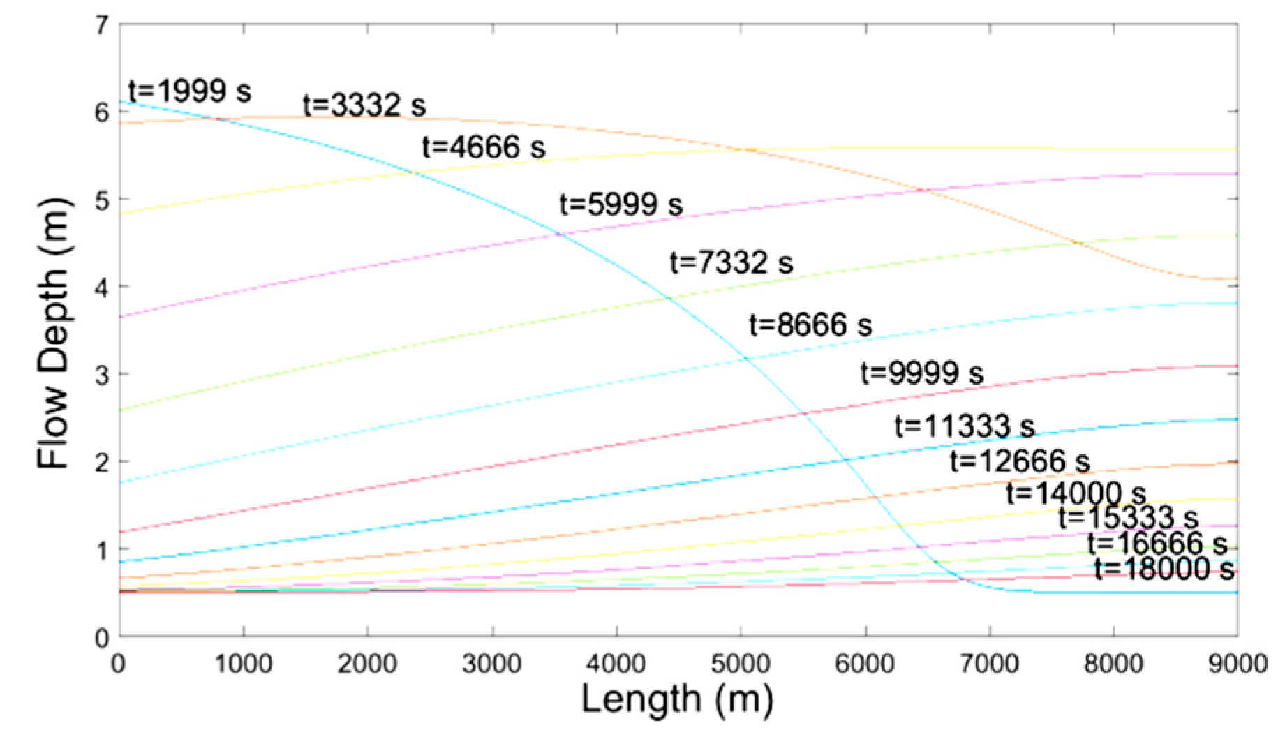
The results are shown in Figure 2, Figure 3, Figure 4, Figure 5, Figure 6, Figure 7 and Figure 8 and consist of the temporal evolution of flow rate (discharge), the flow depth and the average cross-sectional velocity at locations x = 0, x = L/3, x = 2L/3, x = L. The variation of flow depth along the channel at different times is shown in Figure 9.
4.2. Implicit Algorithm
The numerical results from the implicit and the explicit algorithm are presented along with those from HEC-RAS software [17], and Muskingum-Cunge method in this section. More specifically the results regard a 400 m long channel, with symmetrical trapezoidal cross section with 1 m bottom width, 2H:1V side slope, 0.025 Manning coefficient and 0.001 longitudinal bottom slope. The development time of flood wave was 3000 s. At time t = 0 the initial condition was the steady, uniform flow of 10 m3/s, whereas the upstream boundary condition was an inflow hydrograph of the form:
Q(x = 0, t) = Qmin + (Qmax − Qmin)((t/tmax)4.5)exp(4.5(1 − (t/tmax)))
Q(t) is the flow rate at time t, Qmin = 10 m3/s is the initial, uniform flow discharge, Qmax = 50 m3/s and tmax = 800 s are the peak flow rate and the time it occurred respectively, again representing a typical flood hydrograph of Greek rivers. The downstream boundary condition was uniform flow at any time.
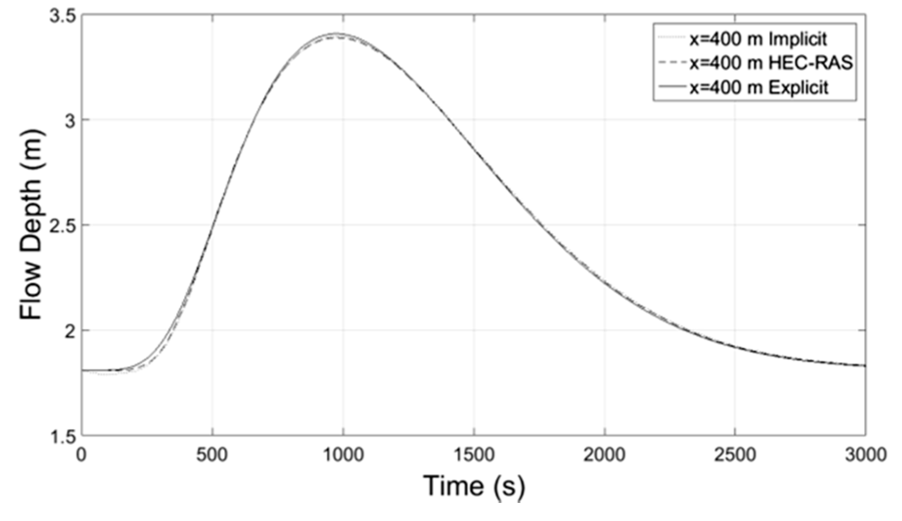
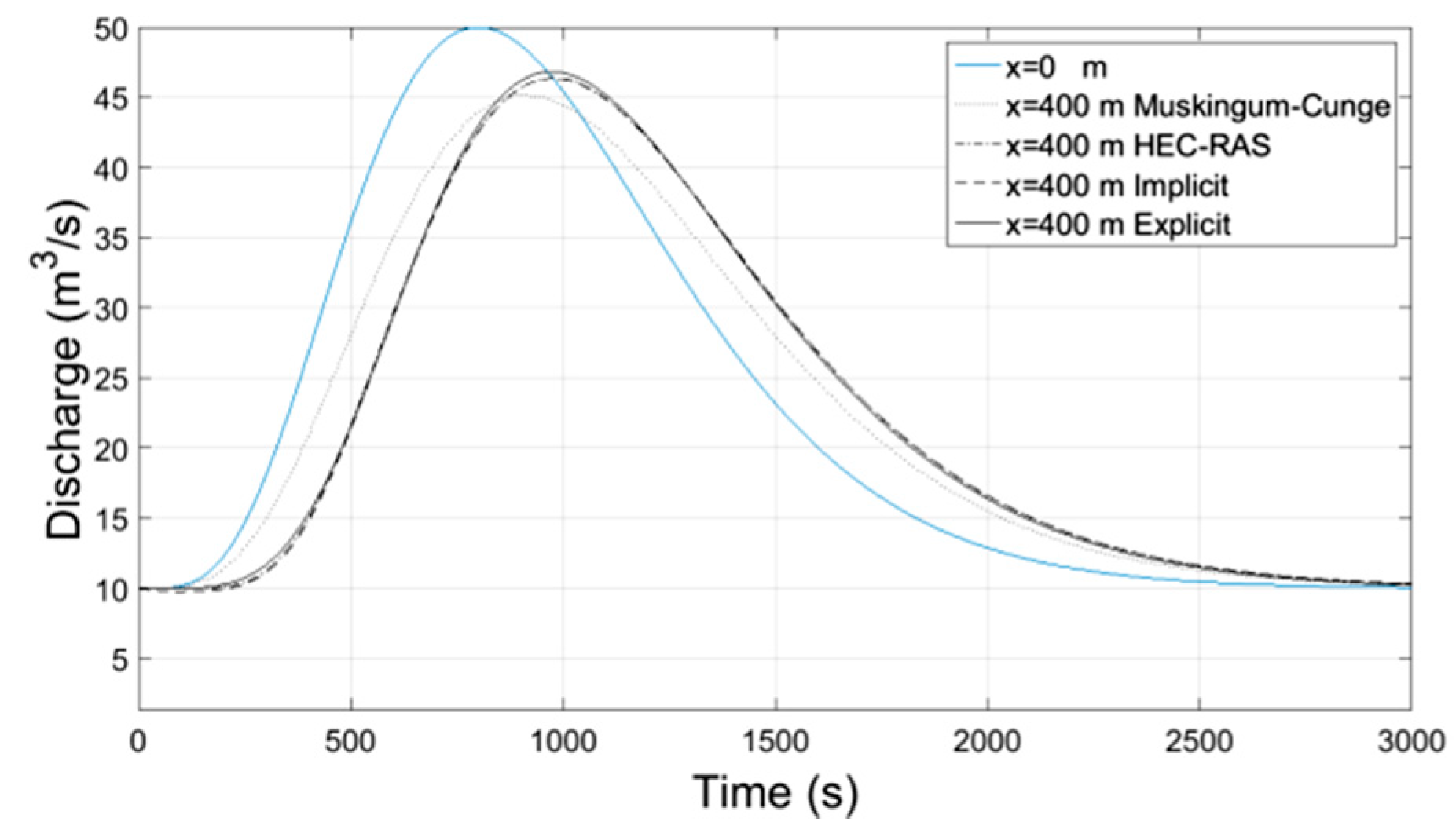
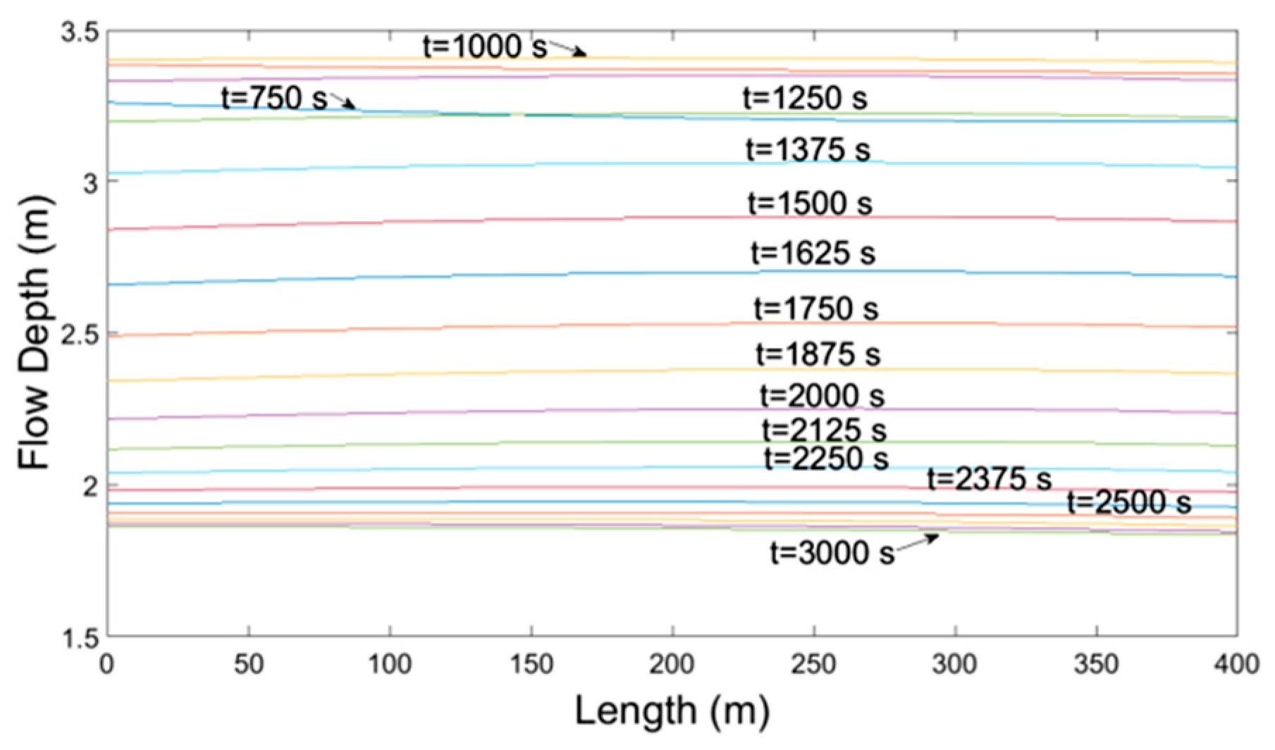
For simplification, the temporal and spatial discretization consisted of 6000 and 10 equidistant nodes respectively for both, the implicit and explicit schemes. The same discretization was used in HEC-RAS calculations, whereas the peak discharge for the Muskingum-Cunge method was selected to be the reference discharge with time step of 60 s. The maximum percentage error of water mass conservation at the downstream end of channel routing hydrographs was 0.21%. The results depicted in Figure 10, Figure 11, Figure 12, Figure 13, Figure 14, Figure 15, Figure 16, Figure 17, Figure 18, Figure 19 and Figure 20 show the temporal evolution of discharge, flow depth and average over the cross-section velocity, at locations x = 0, x = L/3, x = 2L/3, and x = L. The variation of flow depth along the channel at different times is shown in Figure 21.
5. Conclusions
The unsteady, subcritical flow in prismatic open channels of trapezoidal, symmetrical cross section is studied, and the results of four different implementation methods are compared in this manuscript. Two finite difference numerical schemes have been implemented in Matlab® environment, an explicit and an implicit (Preissmann type) scheme, using besides the Courant criterion fine computational grid for satisfying stability of computations. The convergence criterion of the algorithms implemented was the unknown discharge at all times and all the spatial nodes deviate no more than 0.001 m3/s. Due to the long computational time needed for the implicit scheme, a shorter open channel was selected and coarse spatial discretization, so that the number of iterations for a time step did not exceed 30. The four-point implicit scheme was used with a weighting factor 0.5 for precision, whereas stability has not been an issue in this case. The results have been compared to those using the commercial HEC-RAS software and the hydraulic/hydrologic Muskingum-Cunge method.
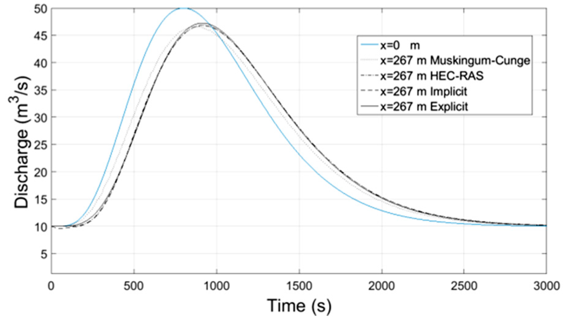
Numerical results of implicit and explicit schemes for trapezoidal channels of length L regarding average cross-sectional velocity and flow depth with time compare well at the locations x = L/3, x = 2L/3 and x = L whereas at the location x = 0 both methods show slightly different results. The results regarding the discharge of explicit scheme and HEC-RAS are almost identical, while the Muskingum-Cunge method overestimates the peak flow and the flow hydrograph at large distances from the inlet (x = 0) deviates from those of the other methods for not showing hysterisis. Additionally in all cases the water mass conservation was confirmed by numerical integration of the resulting hydrographs at all downstream locations showing small percentage errors. All the results from the implicit and explicit finite difference schemes, the Muskingum-Cunge method and HEC-RAS v. 4.1 software compare well.
Additional runs have been implemented by all four previous computational methods for prismatic channels of orthogonal, triangular and circular cross sections. The results are similar to those presented in this paper regarding a symmetrical trapezoid cross section.
To conclude this work, it is evident that a design engineer can use the Muskingum-Cunge hydraulic/hydrologic method that is easy to implement for the preliminary design of long prismatic open channels in unsteady flow, with acceptable accuracy if compared to the outcome of an implicit finite difference scheme or commercial software such as HEC-RAS.
Author Contributions
P.P. and E.D. conceived the idea for a Graduate Thesis and the latter performed all computations and completed her Thesis. E.R. has implemented the numerical algorithms for the explicit and implicit computational schemes and wrote the paper with the contributions of the other two authors.
References
- Liggett, J.A.; Woolhiser, D.A. Difference solutions of shallow-water equation. ASCE J. Eng. Mech. Div. 1967, 93, 39–71. [Google Scholar] [CrossRef]
- Strelkoff, T. Numerical solution of Saint-Venant equations. ASCE J. Hydraul. Div. 1970, 96, 223–252. [Google Scholar] [CrossRef]
- Preissmann, A. Propagation Des Intumescences Dans Les Canaux e.t., Rivkres. In Proceedings of the First Congress of French Association for Computation, Grenoble, France, 1961; pp. 433–442. [Google Scholar]
- Baltzer, R.A.; Lai, C. Computer simulation of unsteady flows in waterways. ASCE J. Hydraul. Div. 1968, 94, 1083–1117. [Google Scholar] [CrossRef]
- Amein, M. An implicit method for numerical flood routing. Water Resour. Res. 1968, 4, 719–726. [Google Scholar] [CrossRef]
- Amein, M.; Fang, C.S. Implicit flood routing in natural channels. ASCE J. Hydraul. Div. 1970, 96, 2481–2500. [Google Scholar] [CrossRef]
- Strelkoff, T. Numerical solution of Saint-Venant equations. ASCE J. Hydraul. Div. 1970, 96, 223–252. [Google Scholar] [CrossRef]
- Fread, D.L. Techniques for implicit dynamic routing in rivers with tributaries. Water Resour. Res. 1973, 9, 918–926. [Google Scholar] [CrossRef]
- Amein, M.; Chu, H.L. Implicit numerical modeling of unsteady flows. ASCE J. Hydraul. Div. Am. Soc. Civ. Eng. 1975, 101, 717–731. [Google Scholar] [CrossRef]
- Amein, M. Streamflow routing on computer by characteristics. Water Resour. Res. 1966, 2, 123–130. [Google Scholar] [CrossRef]
- Streeter, V.L.; Wylie, E.B. Hydraulic Transients; No. BOOK; McGraw-Hill: New York, NY, USA, 1967. [Google Scholar]
- Liggett, J.A.; Woolhiser, D.A. Difference solutions of shallow-water equation. ASCE J. Eng. Mech. Div. 1967, 93, 39–71. [Google Scholar] [CrossRef]
- Wylie, E.B. Unsteady free-surface flow computations. ASCE J. Hydraul. Div. 1967, 96, 2241–2251. [Google Scholar] [CrossRef]
- Sevuk, A.S. Unsteady Flow in Sewer Networks. Ph.D. Thesis, Department of Civil and Environmental Engineering, University of Illinois Urbana–Champaign, Urbana, IL, USA, 1973. [Google Scholar]
- Akan, A. Open Channel Hydraulics, 1st ed.; Elsevier: New York, NY, USA, 2006. [Google Scholar]
- HEC-RAS River Analysis System; Version 4.1; US Army Corps of Engineers, Hydrologic Engineering Center (HEC): Davis, CA, USA, 2010.
- Daskalaki, E.B. Hydraulic and Hydrologic Analysis of Unsteady Flow in Prismatic Channels. Graduate Thesis, in partial fulfillment of the requirements for the Postgraduate Degree from the Graduate Program “Water Resources Science and Technology”, of the National Technical University of Athens, Greece, 2017. (In Greek). [Google Scholar]
Figure 1.
Computational grid.

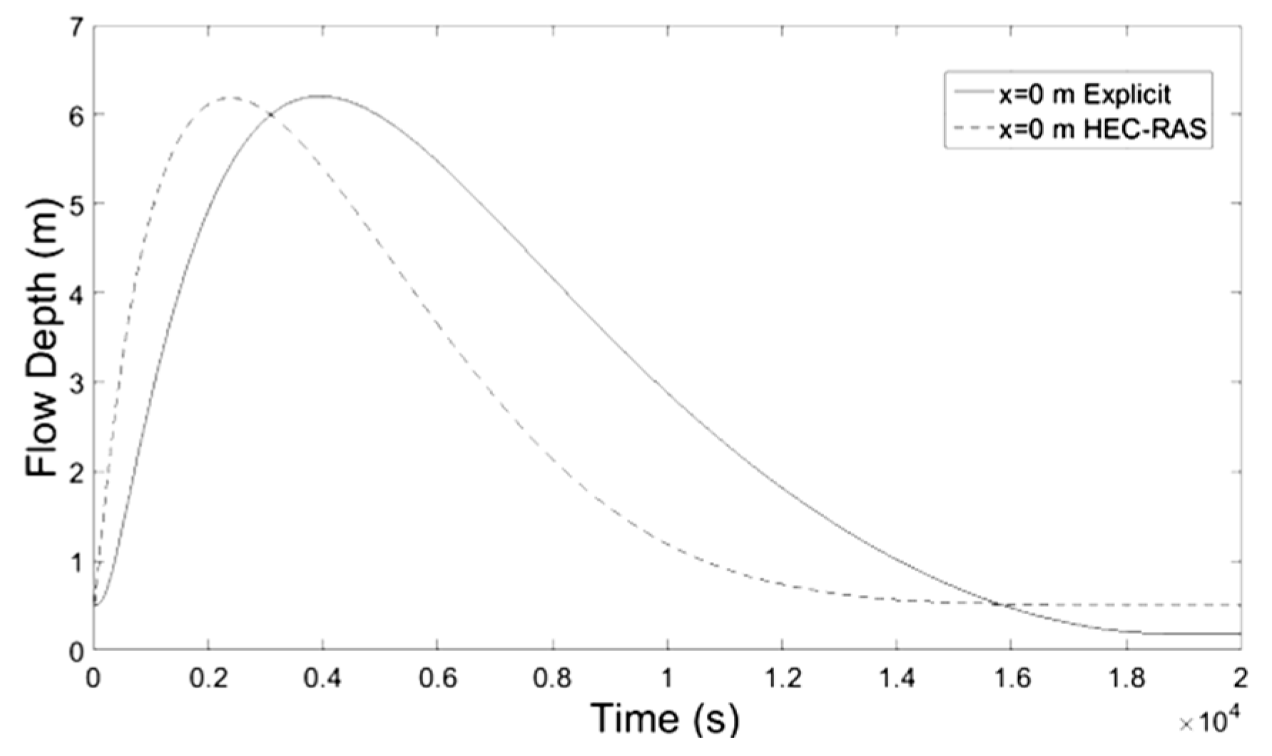
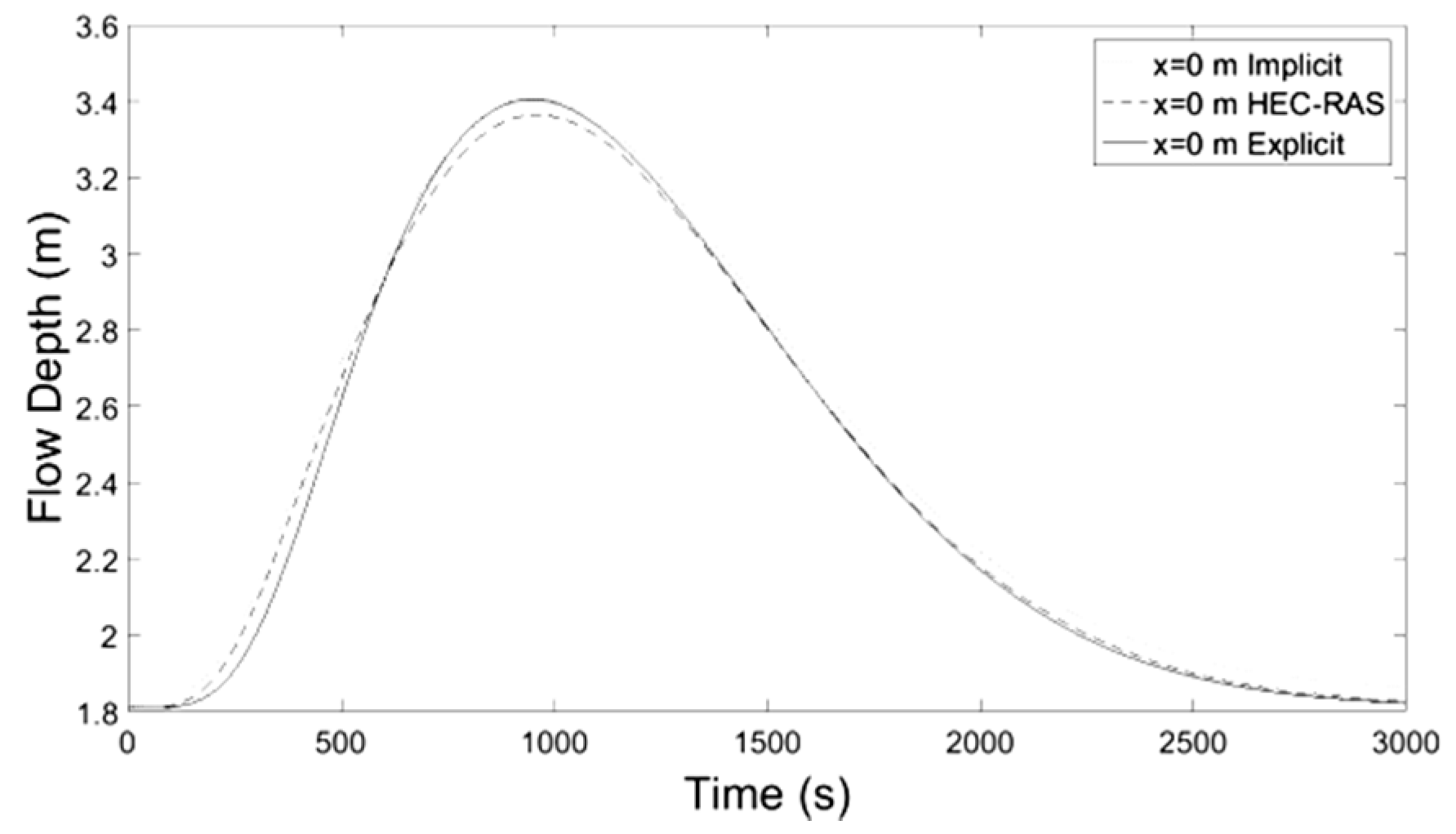
Figure 2.
Flow Depth-Time at x = 0 m.

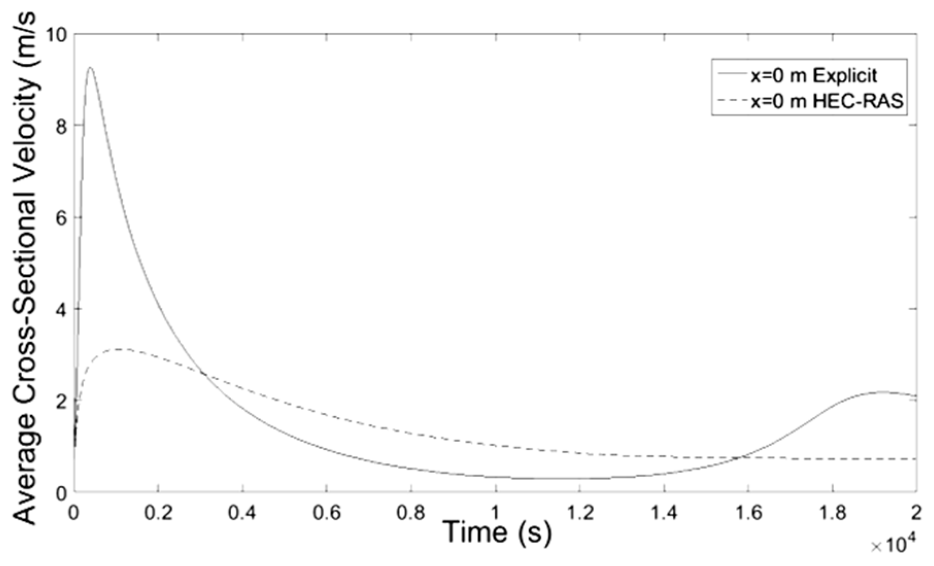
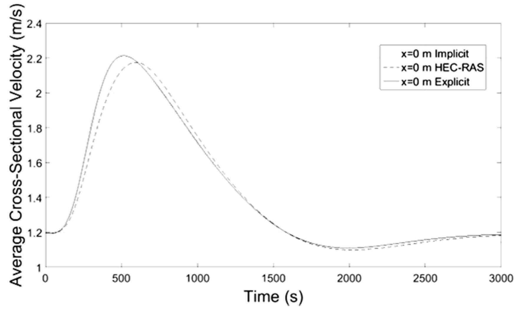
Figure 3.
Average Velocity-Time at x = 0 m.

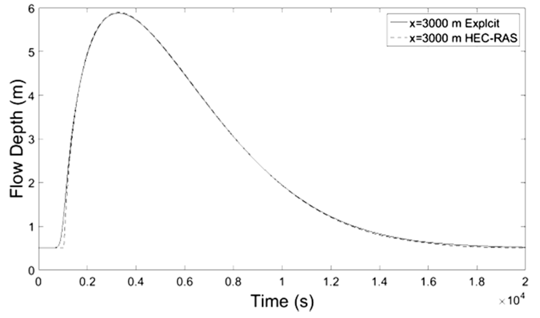
Figure 4.
Flow Depth-Time at x = 3000 m.

Figure 5.
Discarge-Time at x = 3000 m.

Figure 6.
Average Velocity-Time at x = 3000 m.

Figure 7.
Flow Depth-Time at x = 9000 m.

Figure 8.
Discharge-Time at x = 9000 m.

Figure 9.
Flow Depth-Distance at various times.

Figure 10.
Flow Depth-Time at x = 0 m.

Figure 11.
Average Velocity-Time at x = 0 m.

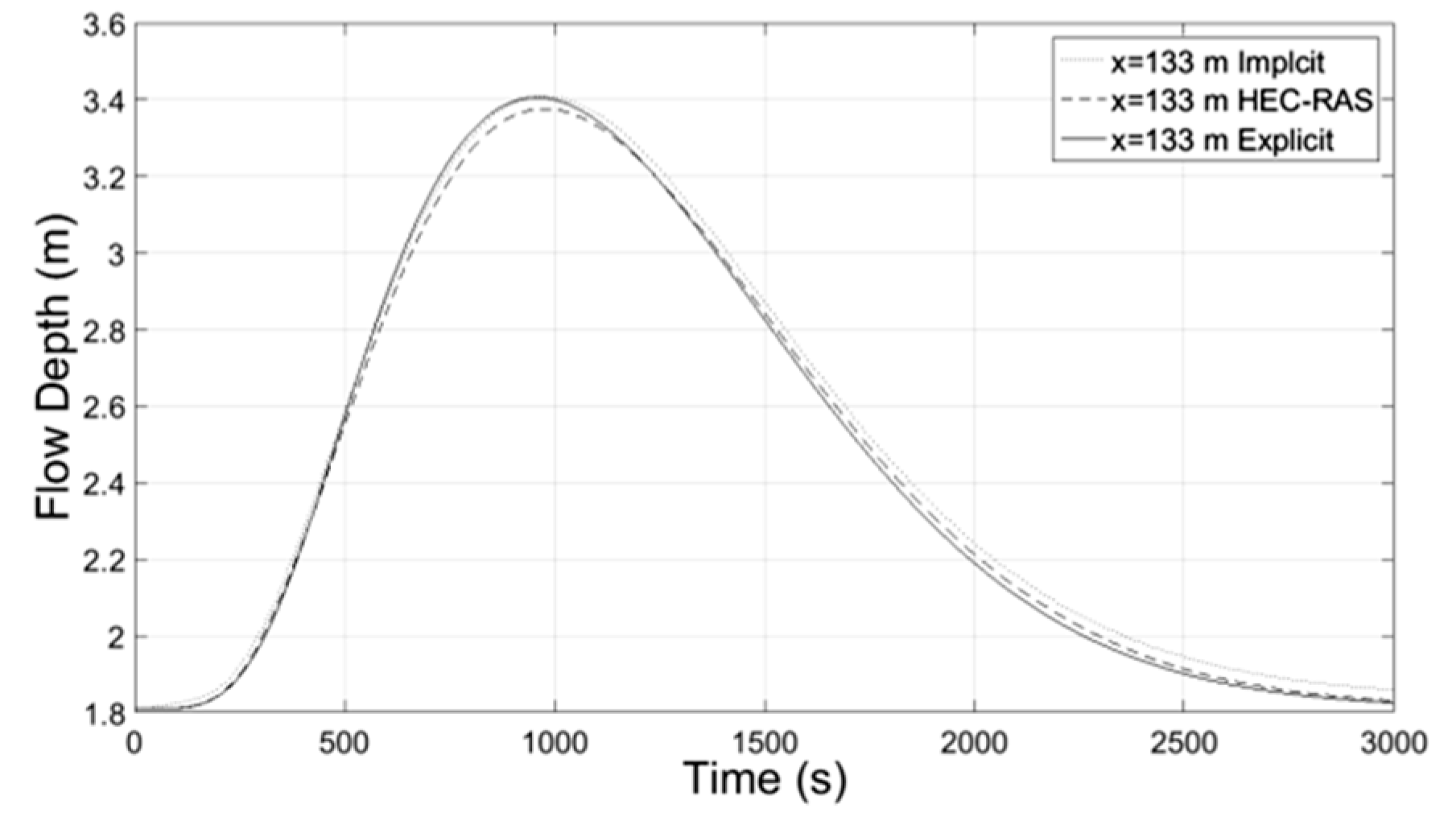
Figure 12.
Flow Depth-Time at x = 133 m.

Figure 13.
Discharge-Time at x = 133 m.

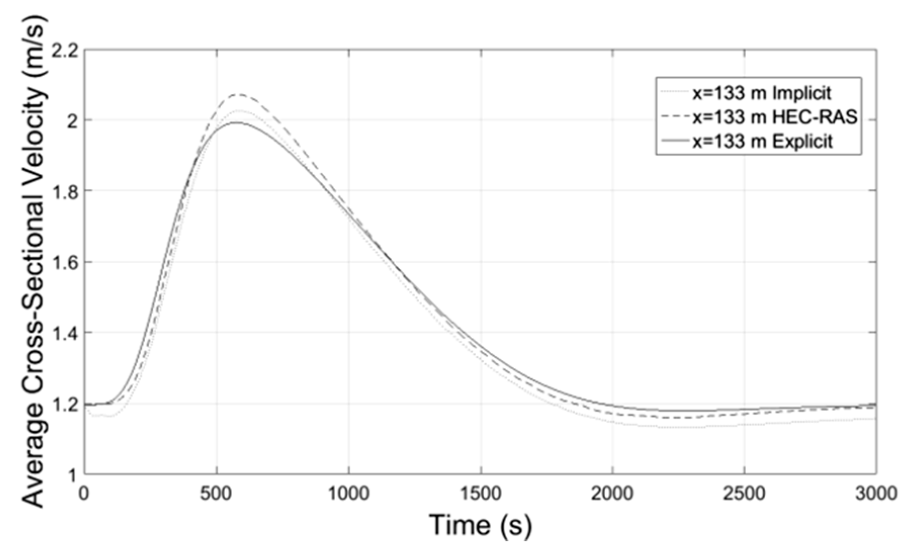
Figure 14.
Average Velocity-Time at x = 133 m.

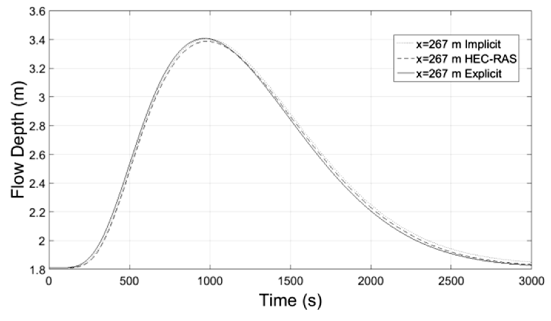
Figure 15.
Flow Depth-Time at x = 267 m.

Figure 16.
Discharge-Time at x = 267 m.

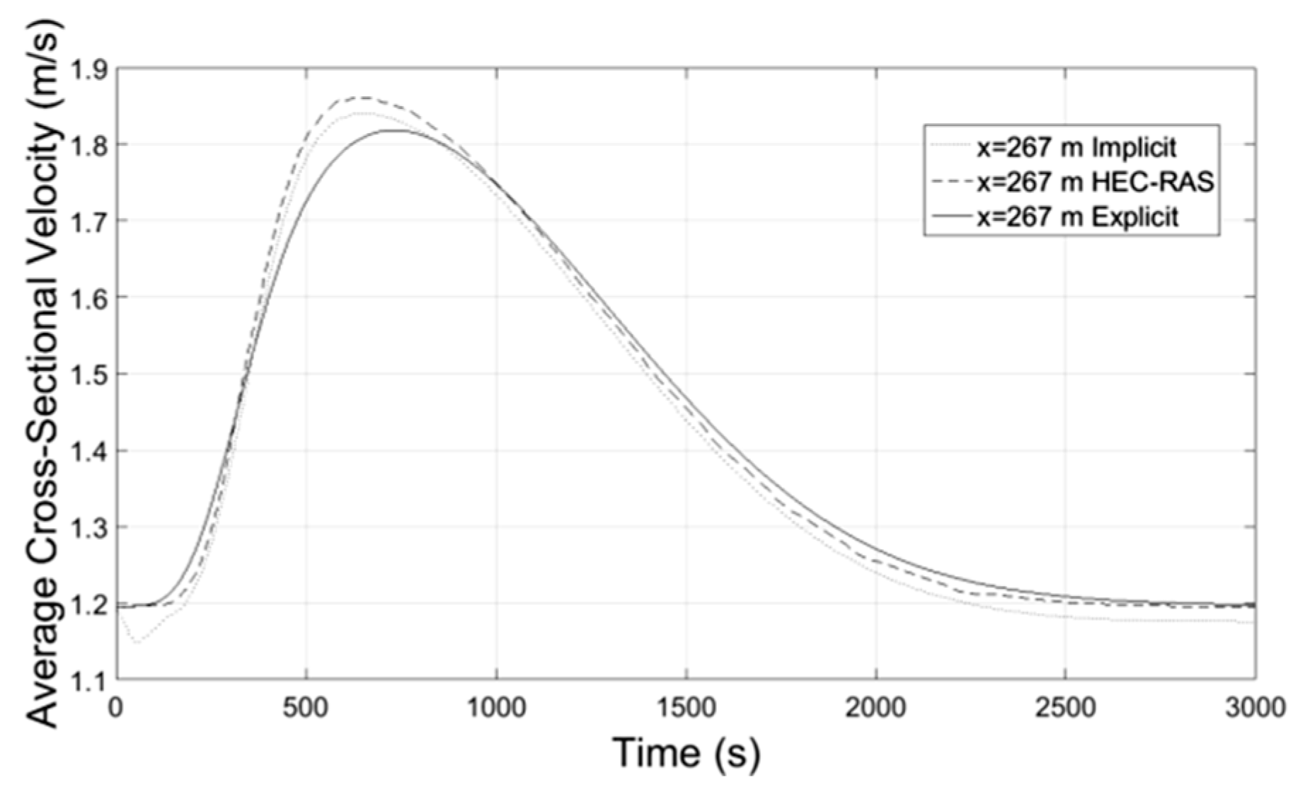
Figure 17.
Average Velocity-Time at x = 267 m.

Figure 18.
Flow Depth-Time at x = 400 m.

Figure 19.
Discharge-Time at x = 400 m.

Figure 20.
Average Velocity-Time at x = 400 m.

Figure 21.
Flow Depth-Distance at various times.

Publisher’s Note: MDPI stays neutral with regard to jurisdictional claims in published maps and institutional affiliations. |
© 2018 by the authors. Licensee MDPI, Basel, Switzerland. This article is an open access article distributed under the terms and conditions of the Creative Commons Attribution (CC BY) license (https://creativecommons.org/licenses/by/4.0/).
Share and Cite
MDPI and ACS Style
Retsinis, E.; Daskalaki, E.; Papanicolaou, P. Hydraulic and Hydrologic Analysis of Unsteady Flow in Prismatic Open Channel. Proceedings 2018, 2, 571. https://doi.org/10.3390/proceedings2110571
AMA Style
Retsinis E, Daskalaki E, Papanicolaou P. Hydraulic and Hydrologic Analysis of Unsteady Flow in Prismatic Open Channel. Proceedings. 2018; 2(11):571. https://doi.org/10.3390/proceedings2110571
Chicago/Turabian StyleRetsinis, Eugene, Erna Daskalaki, and Panos Papanicolaou. 2018. "Hydraulic and Hydrologic Analysis of Unsteady Flow in Prismatic Open Channel" Proceedings 2, no. 11: 571. https://doi.org/10.3390/proceedings2110571