Predictive Dynamic Simulation of Seated Start-Up Cycling Using Olympic Cyclist and Bicycle Models ^†

Abstract

Predictive dynamic simulation is a useful tool for analyzing human movement and optimizing performance. Here it is applied to Olympic-level track cycling. A seven degree-of-freedom, two-legged cyclist and bicycle model was developed using MapleSim. GPOPS-II, a direct collocation optimal control software, was used to solve the optimal control problem for the predictive simulation. The model was validated against ergometer pedaling performed by seven Olympic-level track cyclists from the Canadian team. The simulations produce joint angles and cadence/torque/power similar to experimental results. The results indicate optimal control can be used for predictive simulation with a combined cyclist and bicycle model. Future work needed to more accurately model an Olympic cyclist and a standing start is discussed.

1. Introduction

Over the years, significant work has been put into optimizing track cycling performance by studying the effects of various bicycle designs and cycling techniques. Predictive computer simulation is useful in this regard because it allows for numerous trials under various conditions in a relatively short period of time. The development of a predictive dynamic simulation of cycling allows for various aspects of cycling such as seat and handlebar positions, gear ratios, pedaling rates and general biomechanical technique to be tested much more quickly than with experiments.

Performing predictive simulations using forward dynamics is useful because it does not rely on any previous data. There are two main ways to drive a biomechanical model when using forward dynamics. One is to include individual muscles and to activate them using muscle excitations. Using forward dynamics on a musculoskeletal level allows one to identify individual muscle contributions and investigate muscle coordination [1,2]. However, this can become computationally intensive when using optimal control methods because of the increased number of state variables. An alternative is to use applied torques to represent the combination of muscle forces on a joint. This reduces the number of variables and simplifies the optimal control problem. Joint torque models have been implemented extensively in predictive simulation of human movement, especially with sports applications [3,4].

A commonly used approach in predictive simulations of human movement is to employ optimal control methods. Optimal control using direct collocation has previously been applied to pedaling, which is ideal for such methods due to the constrained nature of the movement [5]. Zignoli et al. recently used optimal control with a joint torque-driven model for predictive dynamics of submaximal cycling [6]. Raasch et al. used optimal control with a musculoskeletal model for maximal start-up pedaling (i.e., starting with zero velocity) [7]. A common theme among previous dynamic models is that many have focused on ergometer pedaling or steady-state cycling and have used some form of resistive torque or effective inertia to provide the resistance at the crank [1,2,5,6]. They do not model the bicycle itself because, for steady-state cycling and ergometer pedaling, the resistance at the crank can be modelled more easily in the aforementioned ways. There has been limited research done in which both the cyclist and bicycle are modelled.

Modelling the bicycle allows one to incorporate the bicycle dynamics when examining the effects of shifting body positions. This becomes important when considering standing starts in track cycling. Schwab and Meijaard conducted a review on previous bicycle dynamics research, which is largely focused on bicycle stability and control methods for balance and steering [8]. More recently, Bulsink et al. investigated rider stability with a fixed rider and included the Pacejka tire model for wheel-ground contact [9], a novel method for bicycle dynamics. For these models, the rider was fixed or only given upper body movement for stability and not lower limb movement for propulsion.

The purpose of this work was to develop a model of a cyclist and bicycle that can be used for predictive simulations of Olympic-level track cycling using optimal control methods. The model should be able to replicate experimental joint angles for seated start-up pedaling and observe similar patterns in crank torque, cadence, and power. Future work will focus on refining the model to study the technique used in standing starts for the team sprint event. During standing starts, cyclists are off the seat and shift their bodies longitudinally relative to the bike to obtain more efficient positions to generate more torque. The long-term goal is to add upper body movement to the model and use predictive simulations to gain a better understanding of what the optimal full body kinematics might look like for standing starts, including the starting pose.

2. Materials and Methods

The model was developed using MapleSim^® because its multi-domain capabilities allowed the bicycle and cyclist to be modelled in the same software. Additionally, its symbolic processing and optimized code generation capabilities make it an excellent choice for developing and exporting computationally-efficient forward dynamics models.

2.1. Bicycle Model

The bicycle model consisted of four bodies: the rear wheel, the front wheel, the crank and the frame/fork/handlebars. Revolute joints connected the rear wheel to the frame and the front wheel to the fork. The crank was modelled as a single link connected to the frame by a revolute joint. The rear wheel motion was connected to the crank motion with a 4:1 gear ratio that is often used in Olympic-level track cycling. The chain efficiency and bearing efficiency obtained from Lukes et al. were lumped together into a single efficiency parameter for the drive system [10]. The focus for the model was on replicating straight-line cycling so a revolute joint was not included between the frame and fork/handlebars. The bicycle was constrained to remain upright and follow a straight path. These simplifications were made to eliminate the need for steering or balancing controllers. The bicycle model has five degrees of freedom: crank rotation, front wheel rotation, longitudinal and vertical translation, and pitch. The dimensions of the bicycle frame were determined from a Look L96 track cycling bicycle frame obtained from Cycling Canada and from the dimensions given on the Look product website. Moment of inertia and center of mass locations were determined using a SolidWorks model of the bicycle frame. Drag was not considered in this model as the effects are negligible when traveling at low speeds during start-up cycling.

The Pacejka tire model was used for modeling wheel-ground contact. MapleSim contains built-in tire model components that were used for formulating the tire force and moment equations. Pacejka parameters have not been reported for track cycling tires so parameters for road tires from Bulsink et al. were used [9]. Petrone and Giubilato reported wheel structural properties that were used for the appropriate rim parameters [11]. To use the tire models when starting at zero velocity, relaxation lengths have to be included. For simplicity, constant relaxation lengths of 0.3 were used.

2.2. Cyclist Model

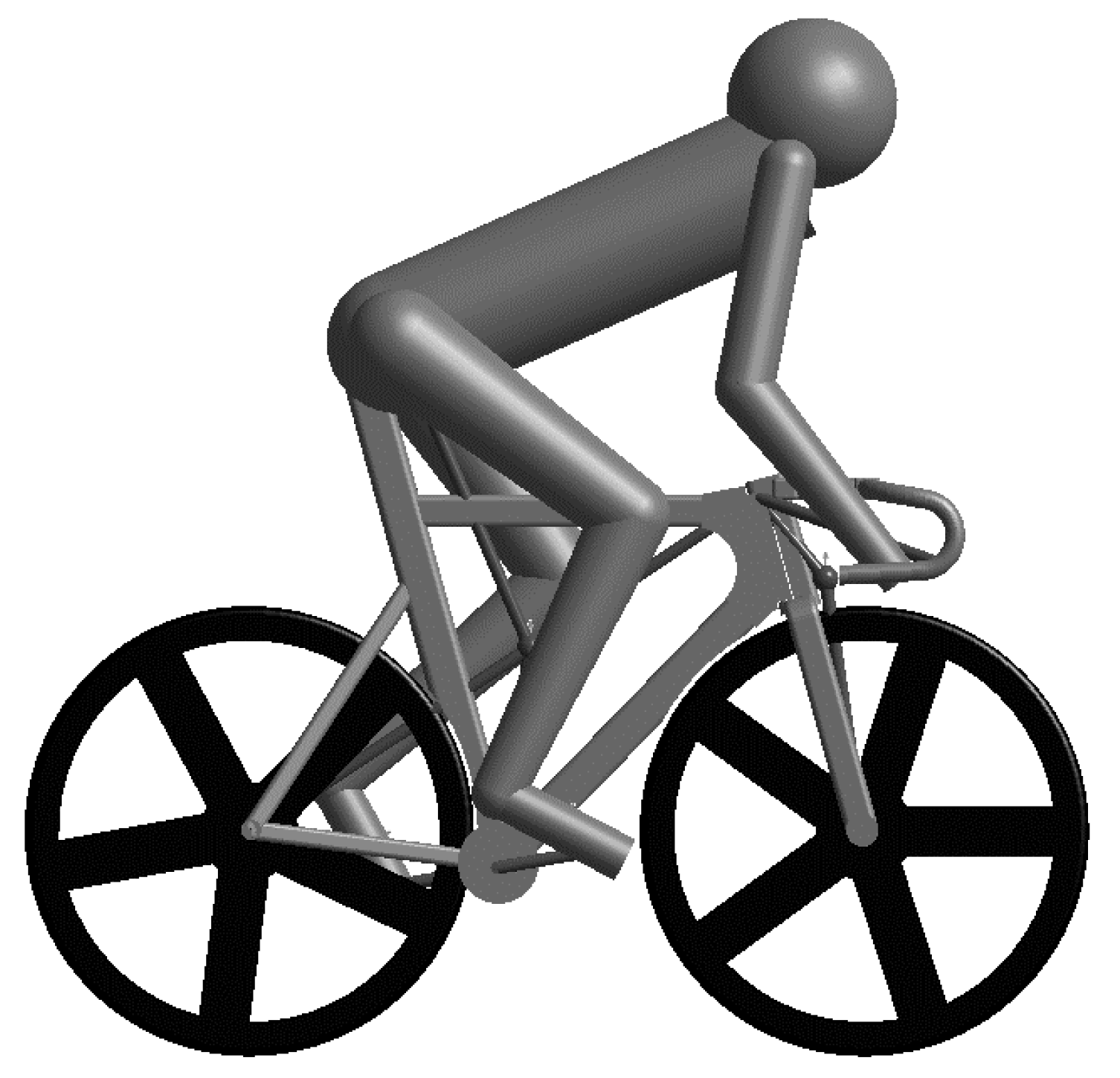
The cyclist model consisted of seven rigid bodies: two feet, two shanks, two thighs, and the head, arms, and trunk (HAT) (Figure 1). The head, arms, and trunk were lumped together and fixed in a constant orientation because, when in a seated position, these segments do not move significantly relative to one another. Revolute joints were used to represent the hips, knees, and ankles. The hip joints were fixed at the location of the seat as the rider was assumed to remain seated while pedaling. The rider’s feet were clipped into the pedals using toe clips, thus allowing the foot/pedal to be constrained to the crank with a revolute joint. Limb properties including segment length, mass, center of mass location, and moment of inertia were set using anthropometric data from de Leva [12]. The anthropometric and bike properties were set to match one of the subjects (from here on referred to as Cyclist X) in an attempt to match simulation results with experimental results as closely as possible.

The model was driven using active joint torques. Anderson et al. developed a joint torque model for the lower limb that was implemented here [13]. The maximum isometric joint torques were scaled up by 1.5 to represent the lower limb strength of an Olympic track cyclist. There were two separate torques applied to each joint: one flexor torque and one extensor torque, which were added together to get the net active torque. The torque values were scaled at each time point based on the joint angle and angular velocity to represent the muscle force-velocity and force-length relationships. Each joint had a maximum rate of torque development that was based on muscle activation and deactivation time constants used by Balzerson et al. [4]. Passive joint torques were also included for each joint. Riener and Edrich’s model for lower limb passive joint stiffness was chosen based on its ability to take into account adjacent joint angles [14].

2.3. Dynamic Equations and Optimal Control

The cyclist and bicycle together is a closed-chain system. Therefore, the dynamic equations are a system of differential algebraic equations (DAEs) which were converted to ordinary differential equations (ODEs). Maple has a built-in function that converts DAEs to ODEs by differentiating the position constraints twice to convert them to acceleration constraints. The Baumgarte constraint stabilization method was used to limit the accumulation of integration errors for the constraints.

Once dynamic equations were all in the form of ODEs, the GPOPS-II optimal control package was used together with an interior-point optimizer (IPOPT) to solve the optimal control problem. GPOPS-II uses orthogonal collocation, which is a direct optimization method. Initial state guesses were based on the crank angle being at 75° and the bike being stationary. The bounds for joint angles and joint angular velocities were set at values that would not restrict the natural motion of the cyclist. The time duration of the simulation was 6 seconds to match the duration of experimental trials. The objective for the simulations was to achieve the maximum distance in the given time period. This was the objective for the cyclists in the ergometer experiments and represents the objective on the track. Therefore, the following cost function was minimized, where $x_f$ = final distance traveled.

$$J=\frac{1}{x_f}$$

(1)

Other cost functions have been used in optimizing pedaling that include some form of minimization of jerks and/or minimization of joint torques. These were considered but ultimately not used because minimization of these led to less distance covered, which was the ultimate goal.

2.4. Experimental Data and Model Validation

An Optotrak motion capture system was used to collect kinematic data for seven (four male, three female) members of the Canadian Olympic program who take part in the team sprint event. Each cyclist performed maximal start-up cycling in the form of two seated six-second sprints on an SRM ergometer, which measured cadence, torque, and power. This test most closely replicated the model in which the hip position was fixed. To validate the cyclist model, the bicycle model was modified to represent ergometer pedaling. The frame and wheels were removed, the crank location was fixed, and extra inertia was added to the crank to represent the inertia of the flywheel.

3. Results

The ability of the model to simulate track bike and ergometer pedaling was tested using the two models and results are included here. The computation time was 271 min on an Intel^® Core™ i7-6700 CPU at 3.40 GHz for the track bike simulations. Figure 2 contains a comparison of average simulated joint angles for the ergometer and track bike to the average joint angles from the 14 experimental trials as well as the joint angles for Cyclist X.

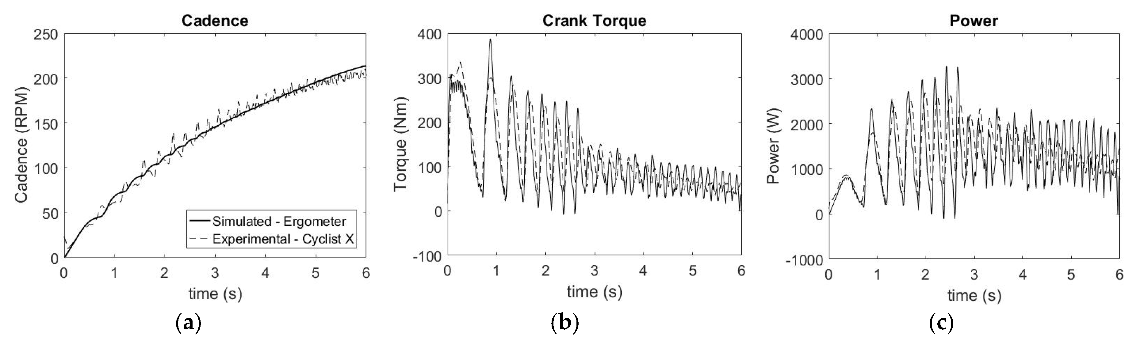
Figure 3 contains a comparison of cadence, torque and power between the simulated ergometer trial and a single experimental ergometer trial for Cyclist X. The simulation was compared with a single trial rather than the average among all trials to show the oscillations and shape of the curves.

Figure 4 shows the net scaled active joint torque for each joint over the course of the full bicycle model simulation. This is the sum of the flexor and extensor torques for each joint.

4. Discussion

Overall, there are similar trends in the joint angles between the ergometer simulations and experiments (Figure 2). There are greater differences seen with the joint angles from the track bike model, but some differences are expected because the resistance experienced at the crank is greater. The oscillations seen in the average joint angles for the bike simulations are largely due to the ankle motion during the initial pedal strokes, when the effective resistance at the crank is highest. Joints were starting with zero torque and zero velocity and needed to overcome the high inertia at the crank so the joint motions were different than at higher speeds.

A primary cause of differences between the simulations and experiments is the constraint on the hip joints to remain fixed. Even during seated pedaling, the hips are moving, which affects the biomechanics. When analyzing the results for the track bike simulations it is important to consider the amount of torque required to generate initial crank movement on a bicycle with a 4:1 gear ratio. Start-up pedaling from a seated position is a difficult task so a cyclist prefers to get up off the seat to attain a mechanically efficient body position and use their mass to aid in driving the pedal downward. In the model, however, the cyclist’s hips are fixed which makes start-up pedaling significantly more difficult because they cannot adjust their body position and use gravity to their advantage. On an ergometer, where the effective inertia is lower, this is not as great an issue.

The cadence, crank torque and power profiles were in a similar range and showed similar oscillatory patterns for the simulation and experiment on the ergometer (Figure 3). The simulated oscillations in the cadence were smaller and not as sharp as in the experimental results. On the other hand, simulated torque oscillations were larger than in experiments. Torque scaling purely based on angular velocity and joint angle means there are peaks where most of the torque is applied, which could be causing the larger torque oscillations. Some of these differences could also be attributed to the simplified method of modelling the ergometer.

Pre-scaled torque showed that each limb was generating the maximum possible torque when the muscles were activated. The net joint torques decreased as the joint angular velocity increased and the joint angle became less optimal for generating torque (Figure 4). As the cyclist increased pedaling rate, the pre-scaled torques did not reach maximum as they did not have time to activate fully before being deactivated again. The ankle motion is generally ~45° out of phase with the hip and knee so at times the ankle torque acts opposite to joint rotation in a stabilizing manner. This eccentric torque causes the active torque to spike high above its maximum isometric value.

5. Conclusions

A two-legged cyclist and bicycle model was developed for predictive simulations via optimal control methods. The predictive simulations can replicate a cyclist performing maximal start-up cycling on an ergometer while in a seated position. Predictive simulations were also performed for start-up cycling on a track bicycle. There are some limitations to the results presented. One is the use of joint torques rather than a full musculoskeletal model for the lower limbs. The additional state variables required make a full musculoskeletal model impractical for use in an optimal control problem. More testing is needed on Olympic-level cyclists as well as their bicycles to ensure the model accurately represents their characteristics. Another shortcoming of the predictive simulation is long CPU times, which is expected for optimal control solution of complex multibody dynamics.

In its current form the model can be a useful tool; however, start-up cycling in track events is not done from a seated position. One reason modelling the bicycle is important for a standing start is that the cyclists shift their body position to minimize the time spent in mechanically inefficient positions. Future work will focus on the addition of upper body movement to accurately model this technique.

References

- Raasch, C.C.; Zajac, F.E. Locomotor strategy for pedaling: Muscle groups and biomechanical functions. J. Neurophysiol. 1999, 82, 515–525. [Google Scholar] [CrossRef] [PubMed]
- Neptune, R.R.; Hull, M.L. Evaluation of performance criteria for simulation of submaximal steady-state cycling using a forward dynamic model. J. Biomech. Eng. 1998, 120, 334–341. [Google Scholar] [CrossRef] [PubMed]
- Yeadon, M.R.; King, M.A. Evaluation of a torque driven simulation model of tumbling. J. Appl. Biomech. 2002, 18, 195–206. [Google Scholar] [CrossRef]
- Balzerson, D.; Banerjee, J.; McPhee, J. A three-dimensional forward dynamic model of the golf swing optimized for ball carry distance. Sport. Eng. 2016, 19, 237–250. [Google Scholar] [CrossRef]
- Thelen, D.G.; Anderson, F.C.; Delp, S.L. Generating dynamic simulations of movement using computed muscle control. J. Biomech. 2003, 36, 321–328. [Google Scholar] [CrossRef]
- Zignoli, A.; Biral, F.; Pellegrini, B.; Jinha, A.; Herzog, W.; Schena, F. An optimal control solution to the predictive dynamics of cycling. Sport Sci. Health 2017, 13, 1–13. [Google Scholar] [CrossRef]
- Raasch, C.C.; Zajac, F.E.; Ma, B.; Levine, W.S. Muscle coordination of maximum-speed pedaling. J. Biomech. 1993, 30, 595–602. [Google Scholar] [CrossRef]
- Schwab, A.L.; Meijaard, J.P. A review on bicycle dynamics and rider control. Veh. Syst. Dyn. 2013, 51, 1059–1090. [Google Scholar] [CrossRef]
- Bulsink, V.E.; Doria, A.; van de Belt, D.; Koopman, B. The effect of tyre and rider properties on the stability of a bicycle. Adv. Mech. Eng. 2015, 7, 1–19. [Google Scholar] [CrossRef]
- Lukes, R.; Hart, J.; Haake, S. An analytical model for track cycling. Proc. Inst. Mech. Eng. Part P J. Sport. Eng. Technol. 2012, 226, 143–151. [Google Scholar] [CrossRef]
- Petrone, N.; Giubilato, F. Methods for evaluating the radial structural behaviour of racing bicycle wheels. Procedia Eng. 2011, 13, 88–93. [Google Scholar] [CrossRef]
- de Leva, P. Adjustments to Zatsiorsky-Seluyanov’s Segment Inertia Parameters. J. Biomech. 1996, 29, 1223–1230. [Google Scholar] [CrossRef]
- Anderson, D.E.; Madigan, M.L.; Nussbaum, M.A. Maximum voluntary joint torque as a function of joint angle and angular velocity: Model development and application to the lower limb. J. Biomech. 2007, 40, 3105–3113. [Google Scholar] [CrossRef] [PubMed]
- Riener, R.; Edrich, T. Identification of passive elastic joint moments in the lower extremities. J. Biomech. 1999, 32, 539–544. [Google Scholar] [CrossRef]
Figure 1.
MapleSim model of a cyclist and bicycle consisting of eleven bodies with seven degrees of freedom. The head, arms, and trunk were fixed and therefore treated as a single body.
Figure 2.
Right leg average joint angles over a pedal stroke for average experimental, Cyclist X experimental, ergometer simulations, and track bike simulations. The shaded area around the “Experimental Average” curve represents the standard deviation. (a) Average hip angle with a constant pelvis angle of 45°, 0° is full extension; (b) Average knee angle, 0° is full extension; (c) Average ankle angle, 0° is perpendicular to shank, positive angle is dorsiflexion.
Figure 3.
Comparison of mechanical outputs at the crank between simulated ergometer pedaling and a single experimental trial for Cyclist X. (a) Cadence; (b) Torque; (c) Power.
Figure 4.
Net active torque at each joint over the course of the simulation using the bicycle model. Vertical dotted lines represent the beginning of each pedal stroke (a) Hip—positive is extension; (b) Knee—positive is flexion; (c) Ankle—positive is plantar flexion.
Publisher’s Note: MDPI stays neutral with regard to jurisdictional claims in published maps and institutional affiliations. |
© 2018 by the authors. Licensee MDPI, Basel, Switzerland. This article is an open access article distributed under the terms and conditions of the Creative Commons Attribution (CC BY) license (https://creativecommons.org/licenses/by/4.0/).
Share and Cite
MDPI and ACS Style
Jansen, C.; McPhee, J. Predictive Dynamic Simulation of Seated Start-Up Cycling Using Olympic Cyclist and Bicycle Models. Proceedings 2018, 2, 220. https://doi.org/10.3390/proceedings2060220
AMA Style
Jansen C, McPhee J. Predictive Dynamic Simulation of Seated Start-Up Cycling Using Olympic Cyclist and Bicycle Models. Proceedings. 2018; 2(6):220. https://doi.org/10.3390/proceedings2060220
Chicago/Turabian StyleJansen, Conor, and John McPhee. 2018. "Predictive Dynamic Simulation of Seated Start-Up Cycling Using Olympic Cyclist and Bicycle Models" Proceedings 2, no. 6: 220. https://doi.org/10.3390/proceedings2060220