Grassmannization of the 3D Ising Model †


1
Dipartimento di Fisica e Astronomia “Ettore Majorana”, Università di Catania, Via S. Sofia, 64, I-95123 Catania, Italy
2
Scuola Superiore di Catania, Università di Catania, Via Valdisavoia, 9, I-95123 Catania, Italy
3
Istituto Nazionale di Fisica Nucleare (INFN), Sezione di Catania, Via S. Sofia, 64, I-95123 Catania, Italy
4
Consorzio Nazionale Interuniversitario per la Struttura della Materia (CNISM), Unità di Catania, Via S. Sofia, 64, I-95123 Catania, Italy
5
Istituto per la Microelettronica e Microsistemi (IMM-CNR), Zona Industriale, VIII strada, 5, I-95121 Catania, Italy
6
Department of Physics, Arnold Sommerfeld Center for Theoretical Physics, Theresienstrasse 37, D-80333 Munich, Germany
*
Author to whom correspondence should be addressed.
†
Presented at the 11th Italian Quantum Information Science conference (IQIS2018), Catania, Italy, 17–20 September 2018.
‡
Current address: School of Physics and Astronomy, University of Birmingham, Edgbaston, Birmingham B152TT, UK.
Proceedings 2019, 12(1), 20; https://doi.org/10.3390/proceedings2019012020
Published: 6 June 2019
(This article belongs to the Proceedings of 11th Italian Quantum Information Science conference (IQIS2018))
Abstract
:The application of Feynman’s diagrammatic technique to classical link models with local constraints seems impossible due to (i) the absence of a free Gaussian theory on top of which the perturbative expansion can be constructed, and (ii) Dyson’s collapse argument, rendering the perturbative expansion divergent. However, we show for the classical 3D Ising model how both problems can be circumvented using a Grassmann representation. This makes it possible to obtain an expansion of the spin correlation function and the magnetic susceptibility in terms of the inverse temperature in the thermodynamic limit, through which the values for the critical temperature and critical index are evaluated within 1.6% and 5.4% of their accepted values, respectively. Our work is a straightforward adaptation of the theory previously developed in an earlier paper.
1. Introduction
The Ising model was introduced in 1920 by Lenz [1] and solved for the first time by Ising in the 1D case [2]. Nearly 20 years later it was solved exactly in the 2D case by Onsager [3] in the thermodynamic limit. For the 3D Ising model no exact solution is known. One typically makes use of Monte Carlo (MC) simulations in order to find its critical temperature and critical indices (although the recently developed conformal bootstrap method [4] can yield results that are two orders of magnitude more precise). MC methods such as the single spin-flip Metropolis algorithm [5] or the superior worm algorithm [6] are applied to finite-size systems. By means of finite size scaling theory one determines the value of the critical indices by demanding that all the rescaled data lines collapse onto each other in the proximity of the critical point (see Ref. [7] for a pedagogical introduction).
Diagrammatic Monte Carlo simulations by contrast simulate the method directly in the thermodynamic limit. The application of diagrammatic Monte Carlo simulations to the 3D Ising model seems at first questionable because (i) there is no free gaussian theory readily available necessary for the application of Wick’s theorem, and (ii) the nature of classical link variables and local constraints is inherently bosonic such that Dyson’s collapse argument, originally formulated for quantum electrodynamics [8], implies a divergent series. One of us (LP) proposed in Ref. [9], together with M. Kiselev, N. V. Prokof’ev and B. V. Svistunov, a theory in which (pairs of) Grassmann variables [10] represent all degrees of freedom of the high-temperature series expansion of the classical partition function (or, more generally, any discrete representation of the system can be used). The resulting expansion is a Feynman series for the spin correlation function, from which the susceptibility can be computed. The susceptibility is known to diverge at the critical point as . Since the series is found to be convergent down to the critical temperature , the convergence radius of the power series gives therefore access to the critical temperature, , and the critical index, . The results presented here have been obtained following the Grassmannization recipe developed by Pollet et al. [9] and by generalizing the code written by Pollet from the 2D case to the 3D case.
2. Results
2.1. Grassmannization of the Ising Model
The approach proposed by Pollet et al. [9] consists of representing the partition function of the 3D Ising model in terms of pairs of Grassmann variables. We do not repeat the development of the formalism here but only discuss the differences of the 3D case compared to the 2D case [9], and introduce notation to make the discussion self-contained. Given a simple cubic lattice, one assigns a set of discrete variables to the links (or, bonds, b), , with a link factor depending on the occupancy number of the link, and one defines a site factor that depends only on the links attached to the jth site. The partition function is then written as , where:
Here, the variables and are Grassmann variables living on the bonds of the lattice. The factors are related to the site factors in a non-trivial way and have to be computed. The easiest expansion we can use for such a computation is the high temperature series expansion of the Ising model partition function, first obtained by Kramer and Wannier [11], for a lattice with N sites, in an external field h:
where , and . One finds for the link factors that and and for the site factors that
These are related to the factors by the following relations,
We can now take the thermodynamic limit and set . The partition function can then be written as follows:
Equation (2) is the starting point for the formulation of the Feynman rules. By Taylor-expanding the non-Gaussian term, the partition function takes the form
and can be evaluated by means of Wick’s theorem. The Feynman rules for the spin correlator at the order are:
- Draw all the n topologically different connected diagrams connecting the origin with site . Any occupied bond contributes 1 to the expansion order n.
- The n bare propagators live on the links (they are local), and are represented by a pair of Grassmann variables. A pair contributes a factor v in magnitude to the weight of the diagram. Propagation lines have no arrows.
- The interaction vertices live on the sites of the lattice, and can be of different type: the origin and end vertex belong to the , or class, the others belong to , or class, whose weights are in accordance with Equation (1). All j legs of the vertices must be connected by propagator lines.
- If a link is multiply occupied, a minus sign occurs when swapping 2 Grassmann variables. The minus signs can equivalently be inferred by identifying all fermionic loops.
- The total weight will be , being P the signature of the exchange permutation, and is the sum of al vertices that are of type j, . It follows that the weight of a diagram is an integer number times .
2.2. Results of the simulations
The details of the algorithm are discussed in [9]. The output of the code, which generates and evaluates all possible Feynman diagrams for the spin correlator up to order 10, is a table shown in Table 1.
The sum of the number of diagrams weighted by the symmetry factor of the cubic lattice contributes to the series coefficients for the expansion of the susceptibility. The series for the susceptibility, obtained after a calculation lasting about one hour on a laptop equipped with an Intel Core i5 2.5 GHz processor with a maximum resident set size of about 9 Gbytes, is
which coincides up to the order under consideration with the result of Campostrini [12].
Since the susceptibility diverges at the critical temperature as , the convergence radius of the power series for can provide information about the critical temperature and the critical index for the model. In order to obtain these, it is sufficient to compare the power series coefficients of with , and to estimate the asymptotic behaviour of the ratio ,
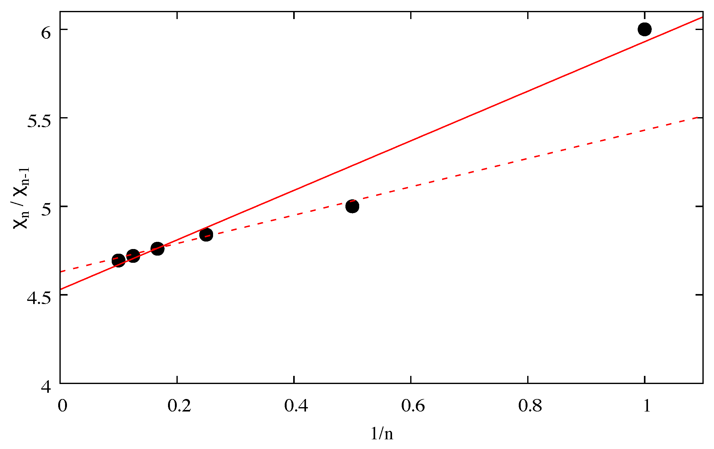
A linear fit of the obtained coefficient ratios as a function of yields the value of the critical temperature and the value of the critical index, as shown in Figure 1.
The results of the fit are such that and , and thus and . These values differ from their known values [12] ( and ) by 1.6% and 5.4%, respectively, but agree within error bars.
In summary, we have successfully benchmarked our Grassmannization approach for the 3D Ising model and thereby obtained the high-temperature series expansion for the spin correlator.
Acknowledgements. We wish to thank M. Kiselev, N. V. Prokof’ev, and B. V. Svistunov for stimulating discussions. LP is supported by the Deutsche Forschungsgemeinschaft (DFG, German Research Foundation) under Germany’s Excellence Strategy – EXC-2111 – 390814868, and FP7/ERC Consolidator grant QSIMCORR No. 771891.
References
- Lenz, W. Beitrag zum Verstandnis der magnetischen Erscheinunge in festen Korpern. Phys. Zs. 1920, 21, 613–615. [Google Scholar]
- Ising, E. Beitrag zur theorie des ferromagnetismus. Zeitschrift für Physik 1925, 31, 253–258. [Google Scholar] [CrossRef]
- Onsager, L. Crystal Statistics. I. A Two-Dimensional Model with an Order-Disorder Transition. Phys. Rev. (Ser. I) 1944, 65. [Google Scholar] [CrossRef]
- El-Showk, S.; Paulos, M.F.; Poland, D.; Rychkov, S.; Simmons-Duffin, D.; Vichi, A. Solving the 3D Ising model with the conformal bootstrap. Phys. Rev. D 2012, 86, 025022. [Google Scholar] [CrossRef]
- Metropolis, N.; Rosenbluth, A.W.; Rosenbluth, M.N.; Teller, A.H.; Teller, E. Equation of State Calculations by Fast Computing Machines. J. Chem. Phys. 1953, 21. [Google Scholar] [CrossRef]
- Prokof’ev, N.V.; Svistunov, B.V. Worm algorithms for classical statistical models. Phys. Rev. Lett. 2001, 87, 160601. [Google Scholar] [CrossRef] [PubMed]
- Sandvik, A.W. Computational studies of quantum spin systems. In AIP Conference Proceedings; AIP: Stockholm, Sweden, 2010; Volume 1297, pp. 135–338. [Google Scholar]
- Dyson, F.J. Divergence of Perturbation Theory in Quantum Electrodynamics. Phys. Rev. 1952, 85, 631–632. [Google Scholar] [CrossRef]
- Pollet, L.; Kiselev, M.N.; Prokof’ev, N.V.; Svistunov, B.V. Grassmannization of classical models. New J. Phys. 2016, 18, 113025. [Google Scholar] [CrossRef]
- Berezin, F.A. The Method of Second Quantization, 1st ed.; Pure and Applied Physics 24; Academic Press: Cambridge, MA, USA, 1966. [Google Scholar]
- Kramers, H.A.; Wannier, G.H. Statistics of the Two-Dimensional Ferromagnet. Part I. Phys. Rev. (Ser. I) 1941, 60. [Google Scholar] [CrossRef]
- Campostrini, M. Linked-cluster expansion of the Ising model. J. Stat. Phys. 2001, 103, 369–394. [Google Scholar] [CrossRef]
Figure 1.
Plot of Equation (3). Black dots are the ratios of the expansion coefficients, while the red solid line is a linear fit. The intercept provides information about , while the slope is related to . Results are in good accordance with the results found in the literature. The red dashed line is a linear fit through the points omitting the one at but it leads to results for and that deviate from the correct answer.


Table 1.
The table shows the number of diagrams connecting the origin with the corresponding site. The second column lists the symmetry factor associated with each site on a cubic lattice.
Table 1.
The table shows the number of diagrams connecting the origin with the corresponding site. The second column lists the symmetry factor associated with each site on a cubic lattice.
| Site | ||||||||||||
|---|---|---|---|---|---|---|---|---|---|---|---|---|
| (1,0,0) | 6 | 0 | 1 | 0 | 4 | 0 | 40 | 0 | 456 | 0 | 6100 | 0 |
| (1,1,0) | 12 | 0 | 0 | 2 | 0 | 16 | 0 | 170 | 0 | 2144 | 0 | 30334 |
| (1,1,1) | 8 | 0 | 0 | 0 | 6 | 0 | 54 | 0 | 648 | 0 | 8840 | 0 |
| (4,0,0) | 6 | 0 | 0 | 0 | 0 | 1 | 0 | 40 | 0 | 1156 | 0 | 24136 |
| (4,1,0) | 24 | 0 | 0 | 0 | 0 | 0 | 5 | 0 | 202 | 0 | 5006 | 0 |
| (4,1,1) | 24 | 0 | 0 | 0 | 0 | 0 | 0 | 30 | 0 | 936 | 0 | 21474 |
| (4,2,0) | 24 | 0 | 0 | 0 | 0 | 0 | 0 | 15 | 0 | 748 | 0 | 18647 |
| (4,2,1) | 48 | 0 | 0 | 0 | 0 | 0 | 0 | 0 | 105 | 0 | 3507 | 0 |
| (4,2,2) | 24 | 0 | 0 | 0 | 0 | 0 | 0 | 0 | 0 | 420 | 0 | 13440 |
| (4,3,0) | 24 | 0 | 0 | 0 | 0 | 0 | 0 | 0 | 35 | 0 | 2219 | 0 |
| (4,3,1) | 48 | 0 | 0 | 0 | 0 | 0 | 0 | 0 | 0 | 280 | 0 | 11060 |
| (4,3,2) | 48 | 0 | 0 | 0 | 0 | 0 | 0 | 0 | 0 | 0 | 1260 | 0 |
| (4,3,3) | 24 | 0 | 0 | 0 | 0 | 0 | 0 | 0 | 0 | 0 | 0 | 4200 |
| (7,0,0) | 6 | 0 | 0 | 0 | 0 | 0 | 0 | 0 | 1 | 0 | 112 | 0 |
| (7,1,0) | 24 | 0 | 0 | 0 | 0 | 0 | 0 | 0 | 0 | 8 | 0 | 802 |
| (7,1,1) | 24 | 0 | 0 | 0 | 0 | 0 | 0 | 0 | 0 | 0 | 72 | 0 |
| (7,2,0) | 24 | 0 | 0 | 0 | 0 | 0 | 0 | 0 | 0 | 0 | 36 | 0 |
| (7,2,1) | 48 | 0 | 0 | 0 | 0 | 0 | 0 | 0 | 0 | 0 | 0 | 360 |
| (7,3,0) | 24 | 0 | 0 | 0 | 0 | 0 | 0 | 0 | 0 | 0 | 0 | 120 |
| (9,0,0) | 6 | 0 | 0 | 0 | 0 | 0 | 0 | 0 | 0 | 0 | 1 | 0 |
| (9,1,0) | 24 | 0 | 0 | 0 | 0 | 0 | 0 | 0 | 0 | 0 | 0 | 10 |
| (10,0,0) | 6 | 0 | 0 | 0 | 0 | 0 | 0 | 0 | 0 | 0 | 0 | 1 |
Publisher’s Note: MDPI stays neutral with regard to jurisdictional claims in published maps and institutional affiliations. |
© 2019 by the authors. Licensee MDPI, Basel, Switzerland. This article is an open access article distributed under the terms and conditions of the Creative Commons Attribution (CC BY) license (https://creativecommons.org/licenses/by/4.0/).
Share and Cite
MDPI and ACS Style
Martello, E.; Angilella, G.G.N.; Pollet, L. Grassmannization of the 3D Ising Model. Proceedings 2019, 12, 20. https://doi.org/10.3390/proceedings2019012020
AMA Style
Martello E, Angilella GGN, Pollet L. Grassmannization of the 3D Ising Model. Proceedings. 2019; 12(1):20. https://doi.org/10.3390/proceedings2019012020
Chicago/Turabian StyleMartello, E., G. G. N. Angilella, and L. Pollet. 2019. "Grassmannization of the 3D Ising Model" Proceedings 12, no. 1: 20. https://doi.org/10.3390/proceedings2019012020