
Design and Performance Analysis of Level Control Strategies in a Nonlinear Spherical Tank


Electrical Engineering Department, Faculty of Engineering, University of Santiago of Chile, Las Sophoras 165, Estación Central, Santiago 9170124, Chile
*
Author to whom correspondence should be addressed.
Processes 2023, 11(3), 720; https://doi.org/10.3390/pr11030720
Submission received: 11 January 2023
/
Revised: 21 February 2023
/
Accepted: 25 February 2023
/
Published: 28 February 2023
Abstract
:This work seeks to contribute to the study of techniques for level control considering a nonlinear plant model. To achieve this goal, different approaches are applied to classical control techniques and their results are analyzed. Fuzzy Logic Control (FLC), Artificial Neural Network (ANN), Adaptive Neuro-Fuzzy Inference System (ANFIS), Model Predictive Control (MPC) and Nonlinear Auto-Regressive Moving Average (NARMA-L2) controllers are designed for the level control of a spherical tank. Subsequently, several tests and scenarios similar to those present in industrial processes are established, while the transient response of the controllers, their performance indices for monitoring the reference value, the rejection of disturbances, the presence of parameter uncertainties and the effects of noise are analyzed. The results show good reference tracking, with a settling time of approximately 5 s for 5 cm and a rise time of less than 4 s. No evidence for steady-state error or overshoot was found and controllers behave positively in the diverse scenarios assessed. The FLC and ANN controllers showed the greatest limitations, while ANFIS, MPC and NARMA-L2 exhibited competitive results considering their transient response and the performance indices calculated.
1. Introduction
Current industrial processes commonly use storage tanks with different geometries, with spherical, conical and cylindrical tanks the most widespread [1]. Industrial processes present nonlinear dynamics and parameters that vary over time. These parameters are affected by uncertainties, disturbances and dead times that deteriorate the performance of the process [2,3,4,5]. Therefore, to increase both product quality and economic benefits, and enhance the overall performance of modern industrial processes, an adequate control of the level of the content in these storage tanks is necessary [6].
In spherical tanks, level control is challenging because the variations presented by the cross-section area and the height of the liquid contained in these tanks generate highly nonlinear dynamics [1,2]. Therefore, the strategies for controlling the liquid level in these tanks should respond adequately to nonlinear systems, such that the liquid level remains stable when perturbations or other events occur that affect the quality and safety of the process or facility.
A procedure frequently used to solve liquid level control in real tank systems has been the design of controllers employing conventional control techniques based on the linearized mathematical model of the tank in question. However, the highly nonlinear dynamics of real industrial processes has hindered the performance of these controllers and motivated the search for alternative solutions, among which are the use of different tuning methods such as Ziegler–Nichols and Cohen–Coon, among others [7,8].
Researchers have proposed the substitution of the classical controller, Proportional-Integral-Derivative (PID), for other variants, such as fractional-order PID (FOPID) [9], Fuzzy FOPID (FFOPID), a PID controller based on Sliding Mode Controller (SMC), Adaptive FOSMC and (FO-PIDSMC) [10,11,12]. In [2], control of the level of a spherical tank is performed through a PI controller using an intelligent optimization method based on Particle Swarm Optimization (PSO/PI); in [13], optimal tuning of a FOPID controller is conducted based on the PSO algorithm. In turn, [14] applies the Model-Free Fractional Order Intelligent Proportional-Integral FOSMC in a water-level tank system.
Other studies dealing with the design of control strategies from SMC controllers are [15,16]. In general, despite a satisfactory performance in a nonlinear and multi-variate system, in practice the SMC controller can damage actuators, thereby limiting its implementation at the industrial level. Another control strategy frequently implemented is Gain Scheduling (GS) and the design of controllers by means of Internal Model Control (IMC) [7,17,18].
In [19], a state error feedback linearization control method paired with a disturbance observer (DOB) and L2 gain is proposed for liquid-level control of a four-tank system. A similar proposal is made by the authors of [20], in which an optimized control strategy is introduced for the control of a four-tank liquid level system. Another control strategy often employed in the industry, primarily for disturbance rejections and with good applicability in tank level control, is cascade control. In [21], a simultaneous tuning of controllers in cascade is conducted based on nonlinear optimization, that seeks to minimize the effect of load disturbance; this tuning succeeded in reducing integral absolute error by 37% in an application for tank level control from the mineral process industry. Other authors who have employed this method are found in [22,23,24,25].
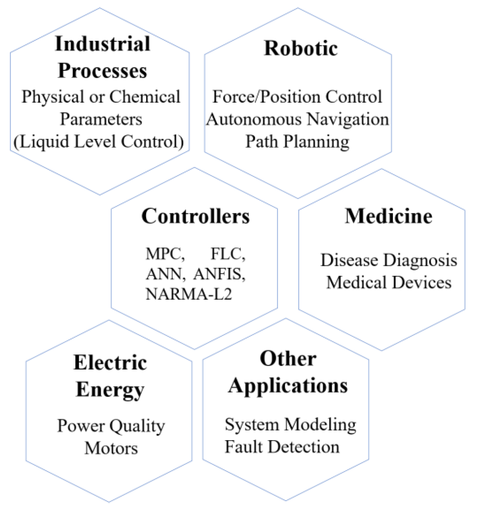
In addition to the control techniques mentioned above, the use of advanced control techniques is widespread, as these offer good performance in systems with complex dynamics. Some of these techniques are common in diverse applications and, according to the literature, most have been implemented in real scenarios, making them attractive for level control. These techniques are Model Predictive Control (MPC), Fuzzy Logic Control (FLC), Artificial Neuronal Network (ANN), Nonlinear Auto-Regressive Moving Average (NARMA-L2) and Adaptive Neuro-Fuzzy Inference System (ANFIS). Figure 1 summarizes some of the main applications in which these controllers have been used in recent years.
It may be observed that advanced control techniques offer suitable solutions for overly complex systems. However, the selection of a specific technique will depend on plant characteristics.
MPC allows the prediction of future responses by the system based on the mathematical model of the plant, adding constraints and tuning variables, and thereby providing robustness to the controller [26]. Easy to understand and apply, MPC is characterized by a good performance in highly nonlinear and multi-variate coupled systems. However, some of the drawbacks of this controller include its low tolerance to noise and high dependence on the plant model for the optimization of its future behavior. Some studies using the MPC controller for level control are [27,28].
The use of fuzzy logic and neural networks extends to several fields. These mathematical algorithms rely on data and the previous knowledge of the system to analyze its behavior. As such, they perform well in the development of control techniques. The FLC controller does not depend on prior knowledge of the plant model. Some applications of this controller in industry are multivariate control for energy savings in a rotary dryer due to a fuzzy multivariable control [29] and as a Fuzzy Decision Support System for the Calibration of Laboratory-Scale Mill Press Parameters [30]. Studies [7,31] employed it for level control. In [32], hybrid control strategies were designed, obtaining the best Fuzzy Based Gain Regulation results for Model Reference Adaptive Controller.
Neural networks provide a representation of a system regardless of its complexity. Their success lies primarily in the quantity and quality of training data. Therefore, the use of signals with frequency and amplitude variation is recommended for capturing the dynamics of the system through neural networks. ANNs are used for optimization, modeling and control of systems [4]. In [33], a neural network-based rapidly exploring random tree algorithm was created for the control of constrained highly dimensional nonlinear liquid level processes. In [34], an approach for the development of a nonlinear MPC (NMPC) controller was proposed using a nonlinear process model based on ANN for liquid level control. An adaptive Sigmoid and Chebyshev network uncertainty modeling-based MPC (ANN-MPC and ACN-MPC) was designed in [35] for the control of real-time uncertain nonlinear systems. Additionally, [36,37] applied data-driven control techniques employing deep learning, while [38] used transfer learning to improve the training of the MPC controller.
The ANFIS controller is most often employed in applications related to electric power and robotics. It has been used efficiently in the control of tank systems in some studies, including [39], in which an ANFIS-based reinforcement learning controller was implemented, and in [40], which dealt with an application for the detection of pH neutralization in multiple tanks. In general, its use has allowed for optimizing results, providing security and reliability due to its robustness against disturbances and changes in system parameters. A discreet use of the NARMA-L2 controller is observed in the literature, despite the good process control it offers [41,42]. In addition, this controller was used for tank level control in [43].
Most of the studies referenced do not use spherical tanks; instead, they present a discrete study of the dynamics of these deposits. Some studies conducted with spherical tanks are [1,2,44,45]. The studies analyzed are generally based on classical control strategies and often use the linearized model of the plant for the design of control strategies. An important limitation is that, in many cases, restrictions related to the physical limits of the actuators and the process in general, safety specifications offered by the manufacturer and the occurrence of limiting situations, such as disturbances or noise, are ignored. Based on these observations, this article seeks to design and study the behavior of these control strategies in a nonlinear spherical tank system. The main contributions of this work are described below:
- Strategies for the level control of a spherical tank are developed considering the nonlinear model of the plant.
- Actual system restrictions are applied, such as flow values based on pump capacity, probable scenarios and the occurrence of disturbances.
- The behavior of the control strategies is assessed in situations close to reality; for example, changes in reference values, the occurrence of disturbances, noise and parametric uncertainties.
- Control strategies are compared in terms of transitory dynamics and performance indices.
The article consists of the five sections. Section 2 describes the system under study, calculates the mathematical expression for the nonlinear model and specifies the variables considered in the experiment. The theoretical foundations of the control strategies designed, as well as their design parameters, are discussed in Section 3. The results obtained and their comparative study are conducted in Section 4. Section 5 presents the conclusions of the results obtained through simulation, as well as potential future work.
2. Description of the System under Study
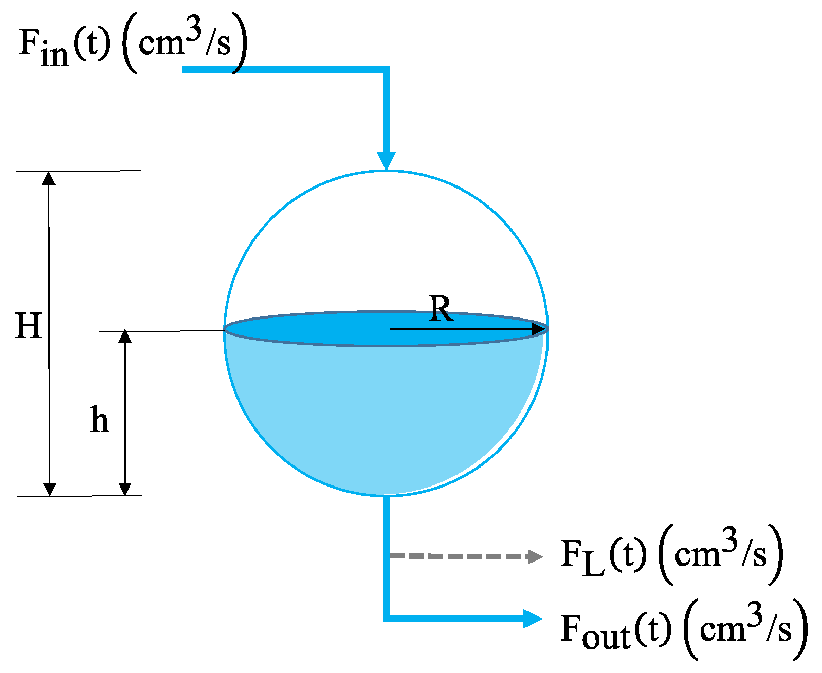
The system employed for the study of the different control strategies is described in Figure 2. Table 1 summarizes the parameters of the spherical tank system as well as its symbology and the values established for the system. In the analysis performed, it is assumed that room-temperature conditions are normal, that the fluid in the tank presents low viscosity and that the tank is open in its upper part (nonpressurized). Additionally, to avoid overloading the water pump, a maximum input flow of 400 cm3/s is established [8]. The output flow, symbolized as FL(t), depends on an auxiliary input for load disturbances; this variable is not considered in order to obtain the mathematical model of the system to be controlled.
Mathematical Model of the System to Be Controlled
The law of conservation of mass states that:
Given that the variation in tank volume equals the area multiplied for the height derivative, and considering the variation in the area of the transversal section of the tank in terms of height, relationship (2) is established. Substituting (2) in (1), expression (3) is obtained.
Output flow can be obtained as shown in (4). Having the spherical cap, Equation (5), the area can be related to the height, as shown in (6).
Finally, substituting (4) and (6) in (3), and clearing the variation of liquid level in the tank, the equation that describes the nonlinear system of the spherical tank is obtained (7):
3. Design of Control Strategies
The following section addresses the theoretical foundations for the design of the control strategies analyzed, as well as the considerations and parameters that were considered for their design.
3.1. Control by Fuzzy Logic
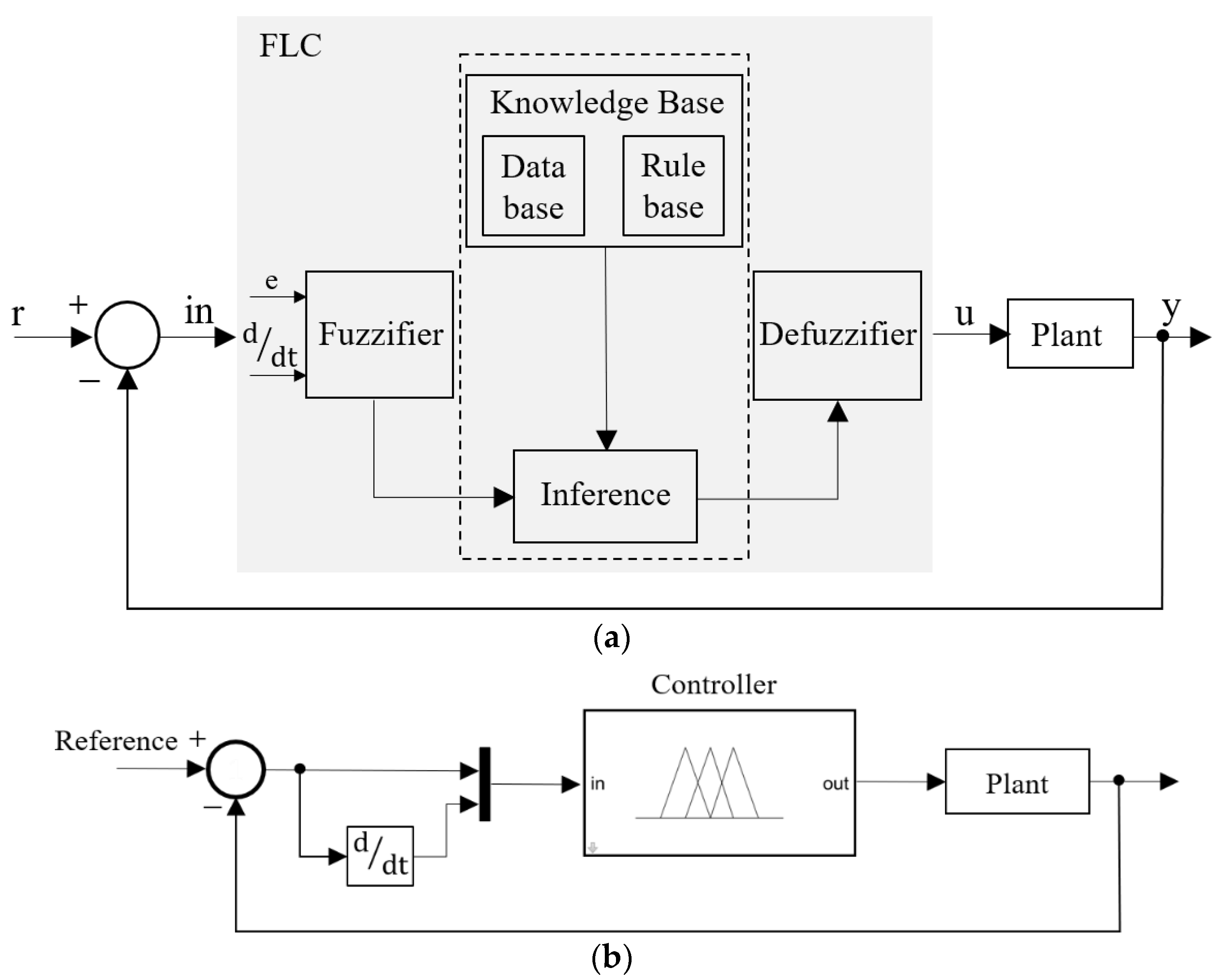
Fuzzy logic was formulated in 1965 by Lotfi A. Zadeh as an alternative to classical logic. Fuzzy logic allows linguistic syntax to be related to numerical data. Fuzzy control permits working with inaccurate information [46], complex dynamics and processes without a simple solution model or an exact mathematical model, hence its emergence as a powerful tool for controlling nonlinear processes such as those developed in the industry [5]. Its design requires knowledge of the process to define its parameters. The structure of fuzzy logic is shown in Figure 3a. The structure of this controller is available in the Fuzzy Logic Toolbox of the MatLab/Simulink software. Figure 3b shows the fuzzy controller created employing the Fuzzy Logic Designer tool.
Input:
- e(t) error: difference between the liquid reference value and the liquid contained in the tank.
- de/dt: derivative of the error in the liquid level present in the tank with respect to the reference value.
- Output: Control action in the valve Fin(t): directly works with the value of the input flow of the tank.
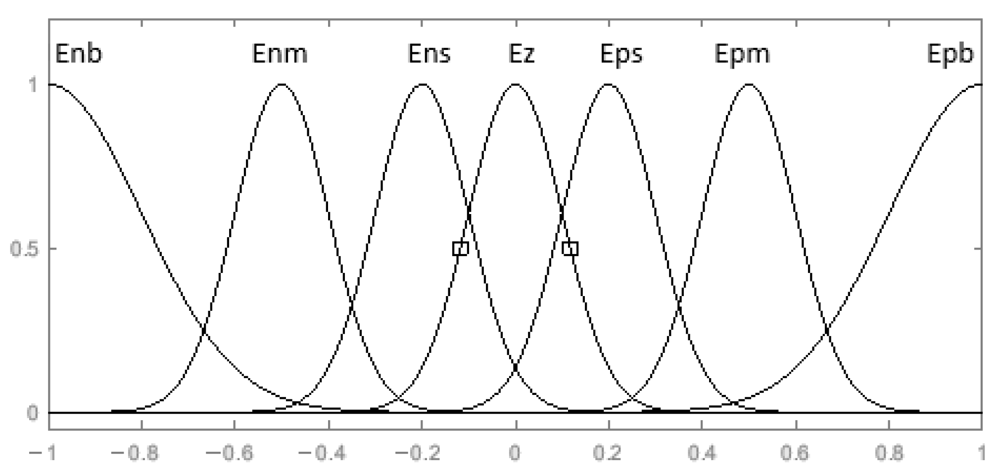
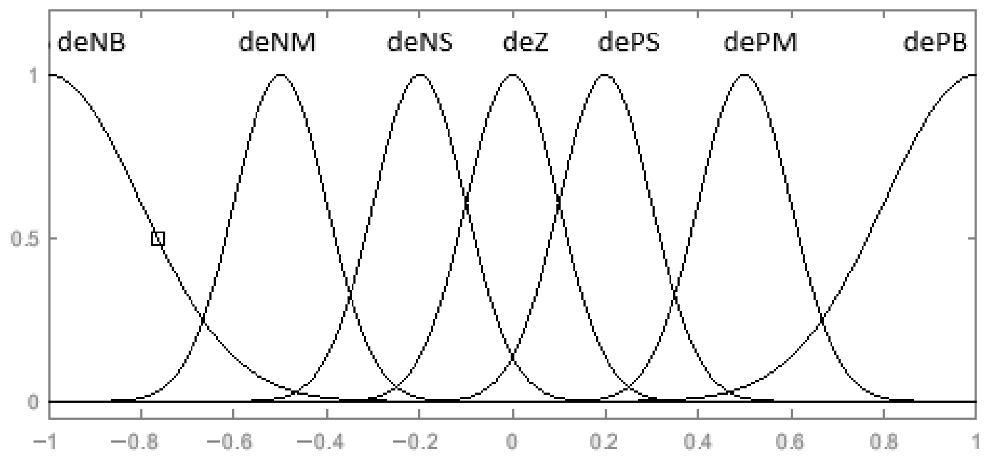
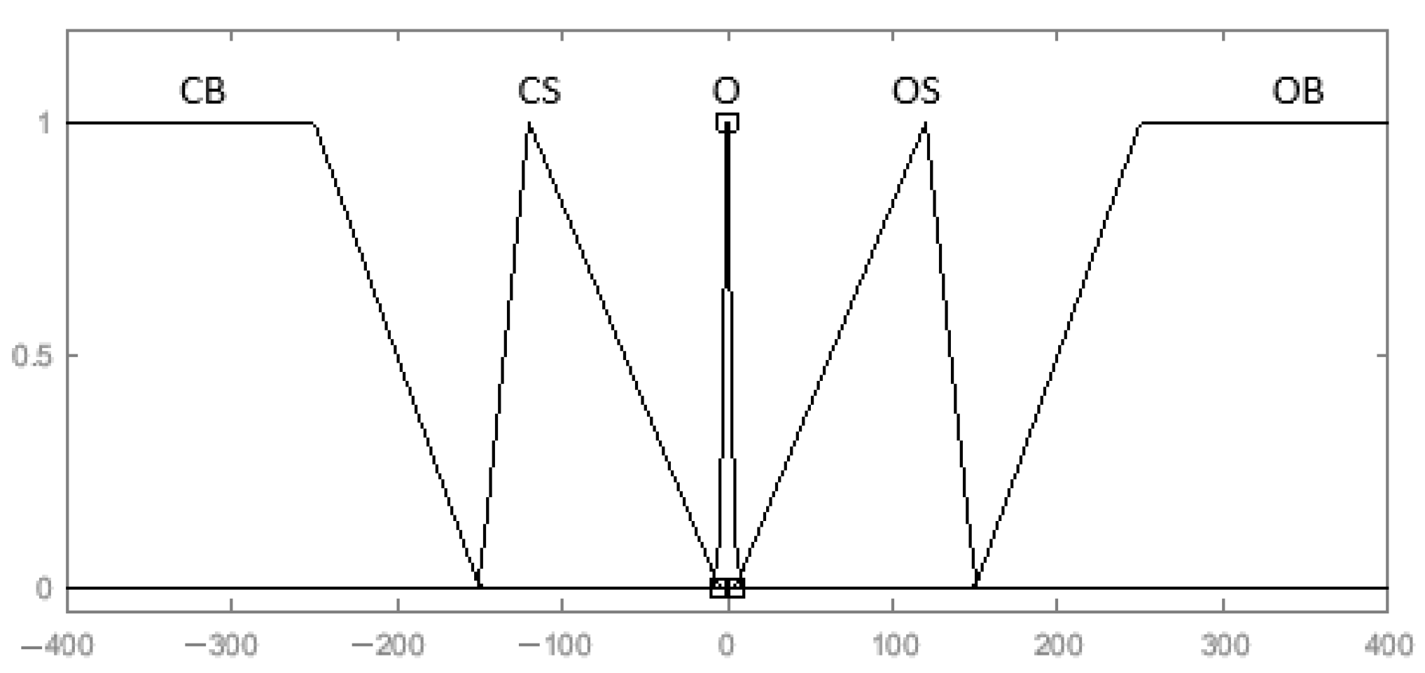
Based on the literature reviewed, the use of five or more membership functions (MFs) is efficient for the controller inputs [47,48]. This allows for a precise control and wide coverage of the entire universe of discourse. Seven Gaussian MFs were established for the input to promote smooth and oscillation-free behavior. At the start, only 5 FMs were used, trapezoidal at the corners and triangular in the center, which are enough to address all cases of filling or emptying the tank and allow for finer control. Considering that controller output is directly related to the flow value that enters the plant and not the voltage of the valve, a discourse universe of ±400 was established. Figure 4, Figure 5 and Figure 6 show the MFs established for input and output, respectively, where N: negative, P: positive, B: large, M: medium, S: small and Z: zero, both for the error and for the derivative of the error. Meanwhile, at the exit, C: closed, O: open, B: large and S: small.
Table 2 shows the stated fuzzy rules, which are assigned based on the knowledge of the system.
3.2. Artificial Neural Network
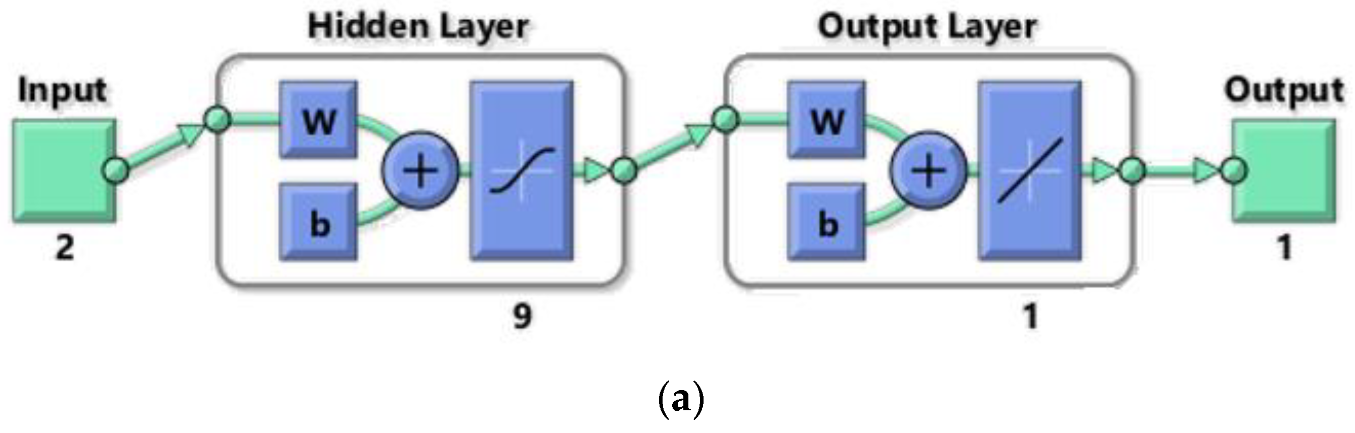
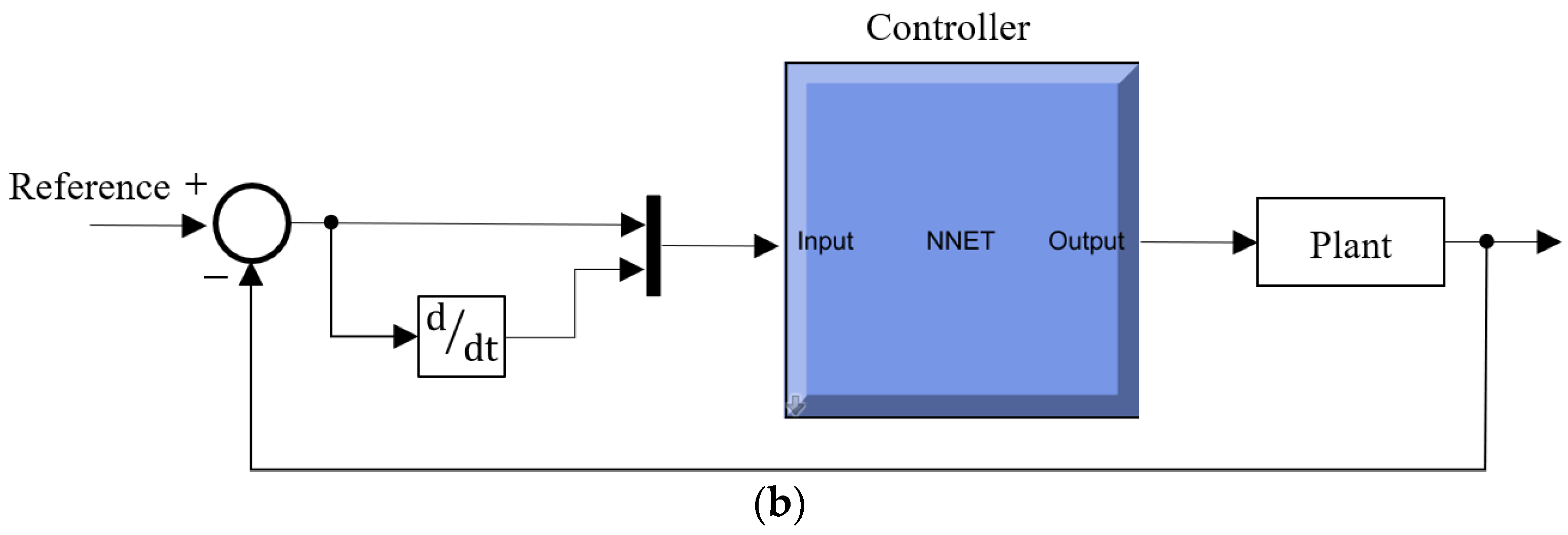
An ANN allows for modeling complex and nonlinear complexes even in the absence of comprehensive knowledge of the same. Therefore, ANNs are considered a valuable tool for the creation of a nonlinear controller [4]. The neural controller was designed using the Neural Network Fitting tool in the MatLab/Simulink software version R2022b. Figure 7 shows the ANN architecture designed.
For the identification of the system, samples of the error and error derivative of the designed fuzzy controller were collected when applying random input signals to the system. At the output, data from the manipulated variable were gathered. As a result, 200,000 samples were obtained; 70% of them were used for the training of the neural controller and the remaining 30% were divided equally between testing and validation of the controller. As observed, 9 neurons were assigned in the hidden layer and 1 in the output layer, as well as 1000 epochs. For the training of the ANN, the Bayesian Regularization algorithm was employed, since it offers good generalization despite its longer training time.
3.3. Adaptive Neuro-Fuzzy Inference System
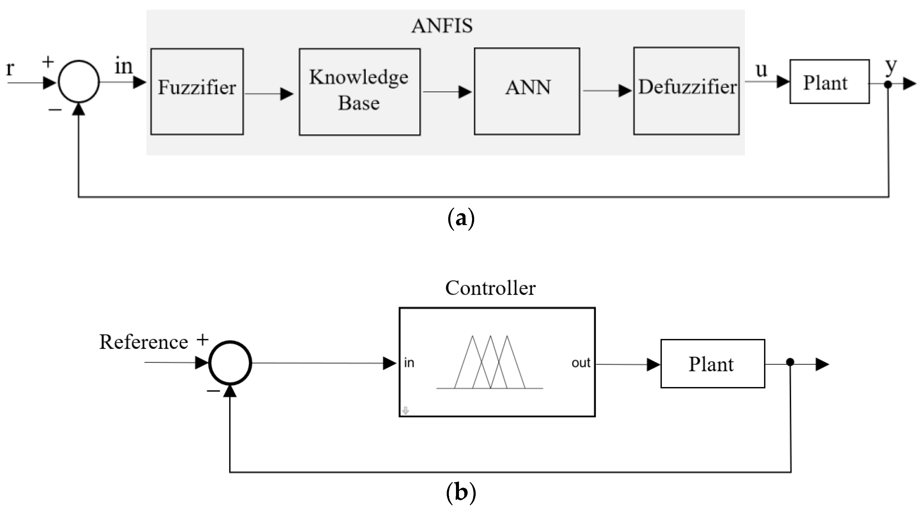
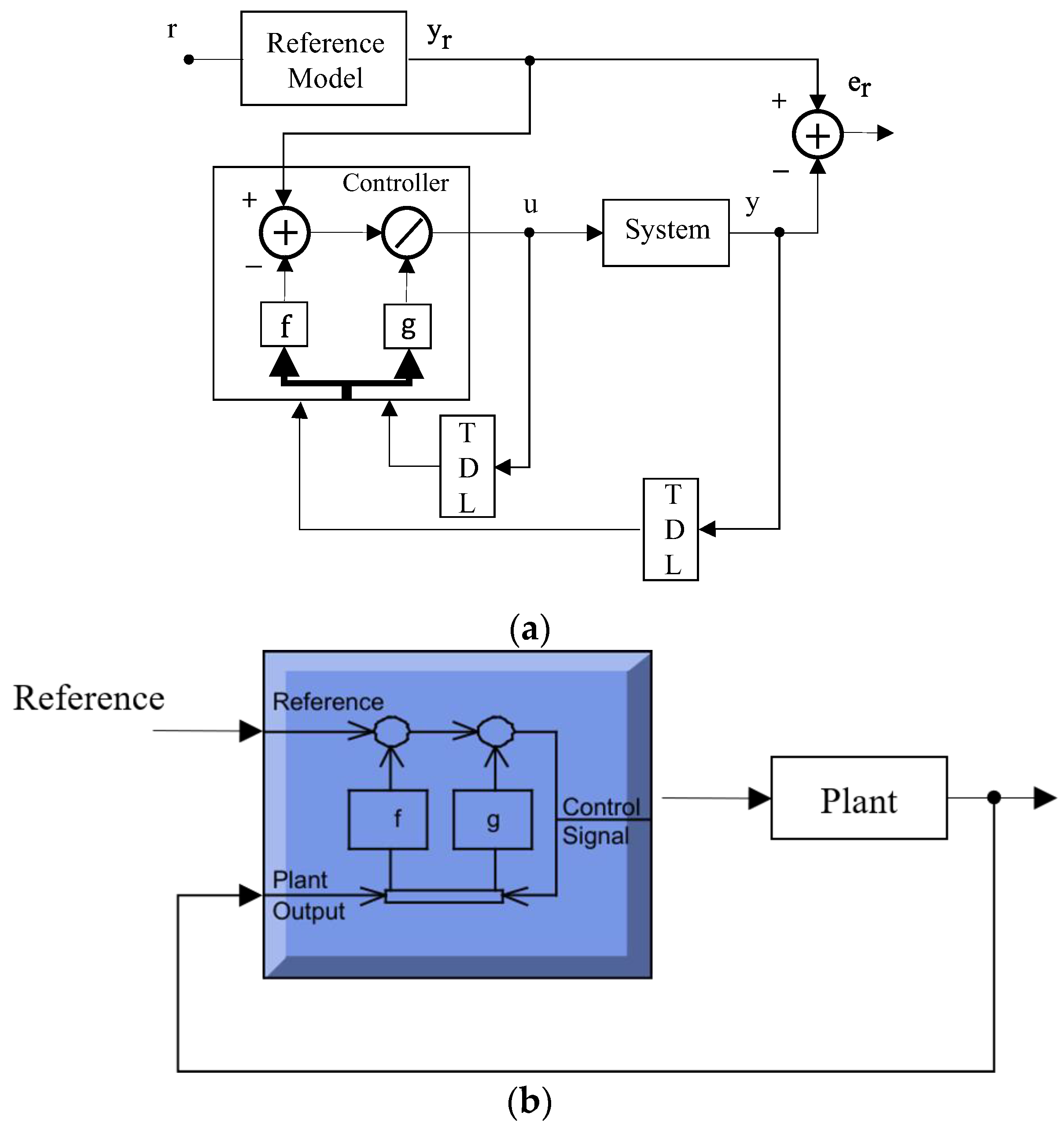
ANFIS is an adaptive neural network designed in the early 1990s, that combines Takagi–Sugeno’s fuzzy inference system with ANNs. The latter component contributes to network learning, while the fuzzy system provides the inference mechanism. Therefore, this technique is considered a universal estimator. In general, ANFIS comprises fuzzy rules and five layers: the input and output layers, and three hidden layers that represent membership functions. This structure enables functions such as fuzzification [15,21]. Figure 8a shows a diagram of its working principle, while Figure 8b presents the block diagram of the controller implementation in Simulink.
For the design of this controller, the Fuzzy Designer application in the MatLab/Simulink software was employed. Additionally, using the fuzblock/Fuzzy Logic Controller, the performance of the controller in the control of the mathematical model of the spherical tank system was analyzed through simulation. To train the controller, the 200,000 samples of the error and the error derivative obtained from the fuzzy controller were used, forming the input vector for ANFIS training. Simultaneously, an output training vector was created with the data of the manipulated variable. The manipulated variable was limited to actual flow values between 0 and 400 cm3/s.
To select the type and quantity of membership functions, a study similar to [22] was conducted. The combinations that offered a lower error and better performance index values were determined. In all cases, 100 epochs, the Grid Partition option and a hybrid optimization method were used. The compared membership functions were generalized bell-shaped membership function (gbellmf), Gaussian membership function (gaussmf), Gaussian combination membership function (gauss2mf), triangular membership function (trimf), Trapezoidal membership function (trapmf), difference between two sigmoidal membership functions (dsigmf), product of two sigmoidal membership functions (psigmf) and Pi-shaped membership function (pimf).
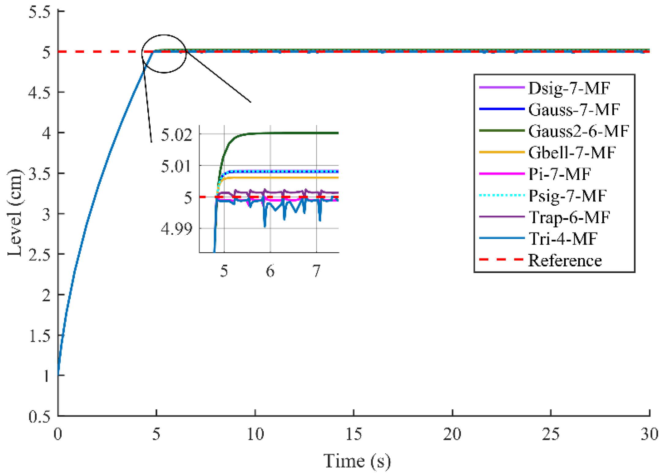
Table 3 shows the results obtained from error, with triangular MFs offering the lowest error. From the controller’s behavior during simulation, it was observed that values of performance indexes better reflected its performance; therefore, higher weight was given to this parameter in the design. The selection of the best combinations for MFs was conducted by jointly analyzing the results for the tracking of the reference value, the transient response and the non-existence of oscillations, as observed in Figure 9.
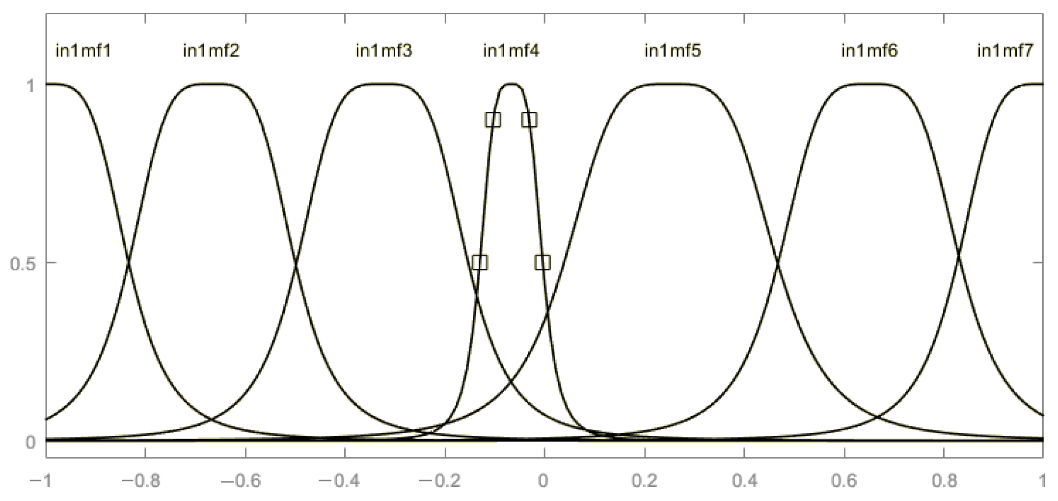
In general, it can be asserted that excellent results are obtained with 6 trapezoidal Traps MF (6 MF), and that Pi (7 MF) and Trimf (4 MF) present small oscillations. Although Gaussian MFs report more discrete performance indices, they do not present oscillations. Therefore, Gbell MFs (7 MFs) achieve better results in general, as shown in Figure 10. The type of ANFIS controller under study uses the Takagi–Sugeno inference system, and reports better performance when employing constant membership functions at the output.
3.4. Model Predictive Control
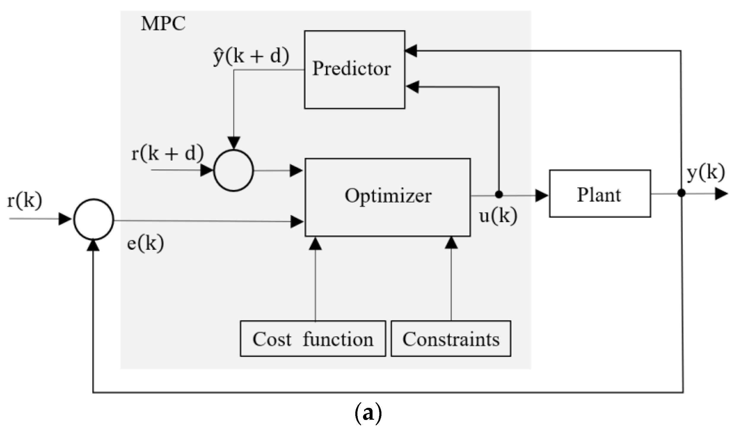
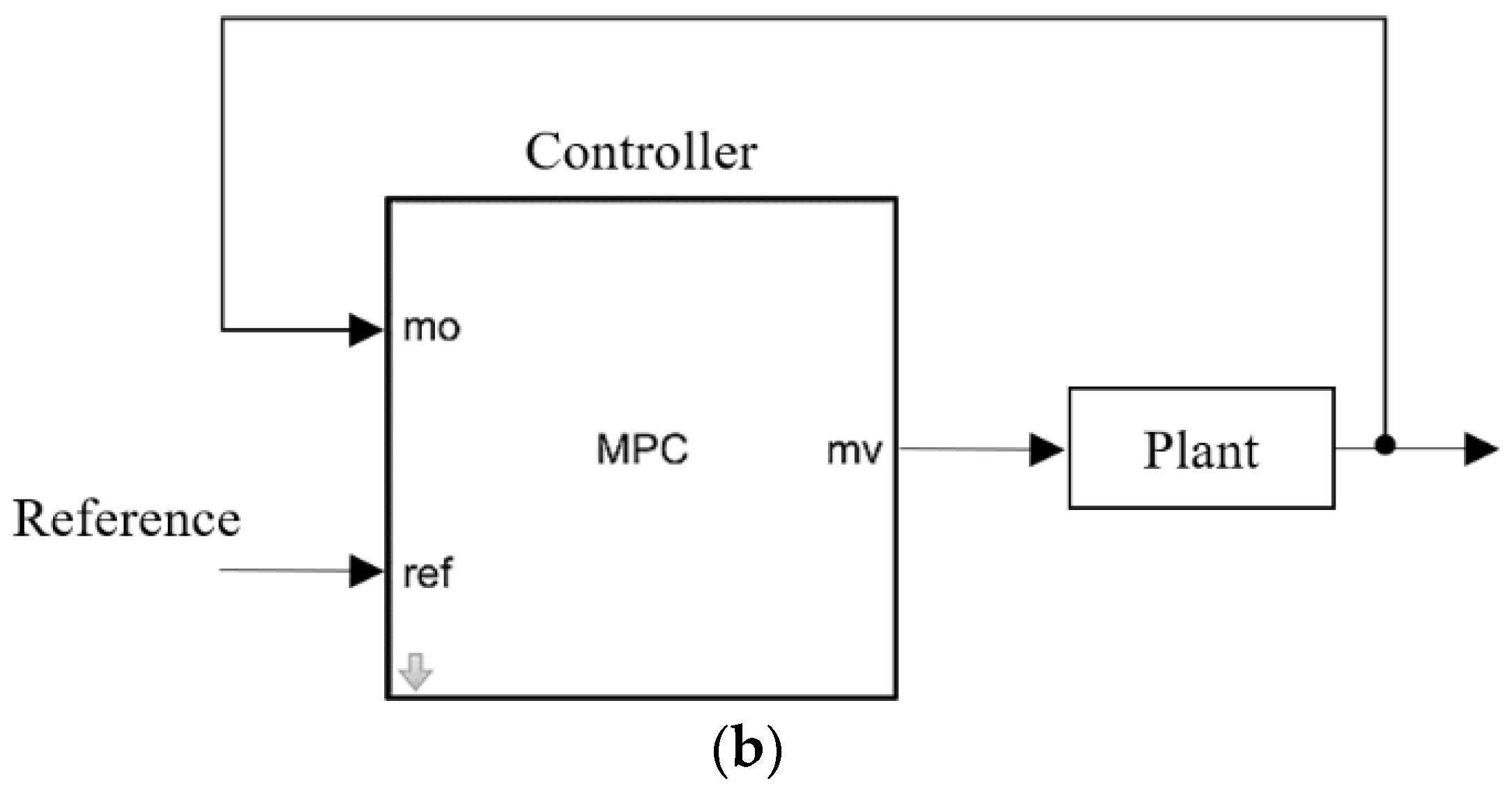
MPC, in general, refers to a set of advance control techniques widely used in the industry, with Generalized Predictive Control (GPC) as its best known formulation [34]. Figure 11a shows a diagram of the principle of operation of the MPC, while Figure 11b presents a generic block diagram of its implementation in Simulink. MPC uses a predictive model of the system to be controlled and a specified prediction horizon to predict the future behavior of the system. Based on this, an open loop optimal control sequence is generated to solve an optimization problem [23]. Some of the common elements used to define an MPC controller are the prediction model, target function and control law.
This controller was designed using the MPC Designer application of the MatLab/Simulink software. Table 4 summarizes the design parameters of the MPC controller.
To obtain a linear model of the plant, the operation point was determined through an optimization method. To this end, input and output constraints for both the flow and the level of the tank were considered. The best optimization results were obtained experimentally using the Nonlinear Least Squares with Projection and the application of the Levenberg–Marquardt algorithm. A fast state estimation and a relatively aggressive close loop were selected. The maximum and minimum flow and liquid level values were assigned based on the initial constraints of the deposit. A sampling time of 0.001 was employed, allowing for adequate modeling of the plant’s dynamic. Thanks to the facilities offered by the simulation software, an adequate value was interactively determined for the control and prediction horizons in order to ensure a fast response without high computational costs, as well as an accurate assignation of weights.
3.5. Nonlinear Autoregressive Moving Average
The central idea in this type of control is to transform the nonlinear system dynamics in linear dynamics by cancelling nonlinearities. Figure 12 shows a block diagram of the NARMA-L2 controller.
The first step to implement this controller is to identify the system to be controlled, for which an ANN representative of the system direct dynamics is trained. A standard mathematical model used to represent nonlinear general systems is the NARMA-L2 model, defined in (8), in which u(k) and y(k) represent the input and output of the system, respectively.
Employing the NARMA-L2 model, a controller represented by expression (9) is obtained, which is applicable to d ≥ 2.
To design a NARMA-L2 neural controller, the Neural Network Toolbox of the MatLab/Simulink software was employed. A sampling interval of 0.001 was established for both system identification and controller design, which favored the modeling of the system. The constraints inherent to the system were also respected in terms of maximum and minimum flow and liquid level values at the input and output, respectively. The identification process yielded 668,300 training samples. Nine hidden layer neurons, 1000 epochs and the Training function trainbr were employed. These parameters were assigned as they offered better experimental performance, with a Mean Squared Error (MSE) of 6.4335 × 10⁻¹³ and a perfect fit of R = 1, as shown in Table 5.
4. Results and Discussions
Several factors can affect the operation of a plant in general, including disturbances, noise and uncertainties. Hence, it is of significant interest to analyze the robustness of the system in the face of these adverse factors. Although disturbances can affect the plant at any point, it is usual to consider supply disturbances at the input of the plant and load/demand disturbances at the measurement point at the output of the plant [50].
The existence of imprecise mathematical models of the system should also be considered. Model inaccuracy is caused by uncertainty in the plant (for example, unknown parameters) or by the simplified representation of the plant dynamics. From a process control perspective, model inaccuracies can be classified into two large groups: structured or parametric uncertainties, and unstructured or unmodeled dynamic uncertainties. The former category refers to inaccuracies in the terms currently included in the model, while the latter category corresponds to inaccuracies in the order of the system [51].
This section deals with the simulation results of liquid level control in a spherical tank considering its nonlinear mathematical model and conditions close to reality. The performance of each control strategy was verified through simulation of different scenarios where the control variable was affected, including changes in the output flow, rain incidence and evaporation of the content in the deposit. For a quantitative assessment of the results of each controller in terms of response quality and error value, which allows for comparing them with one another, several Performance Indexes (PIs) were calculated. Equations (10) and (11) represent the integral square error and its behavior over time. In turn, Equations (12) and (13) represent the integral absolute error and its behavior over time, respectively [52].
Integral Square Error (ISE):
Integral of time multiplied Squared Error (ITSE):
Integral Absolute Error (IAE):
Integral of time multiplied Absolute Error (ITAE):
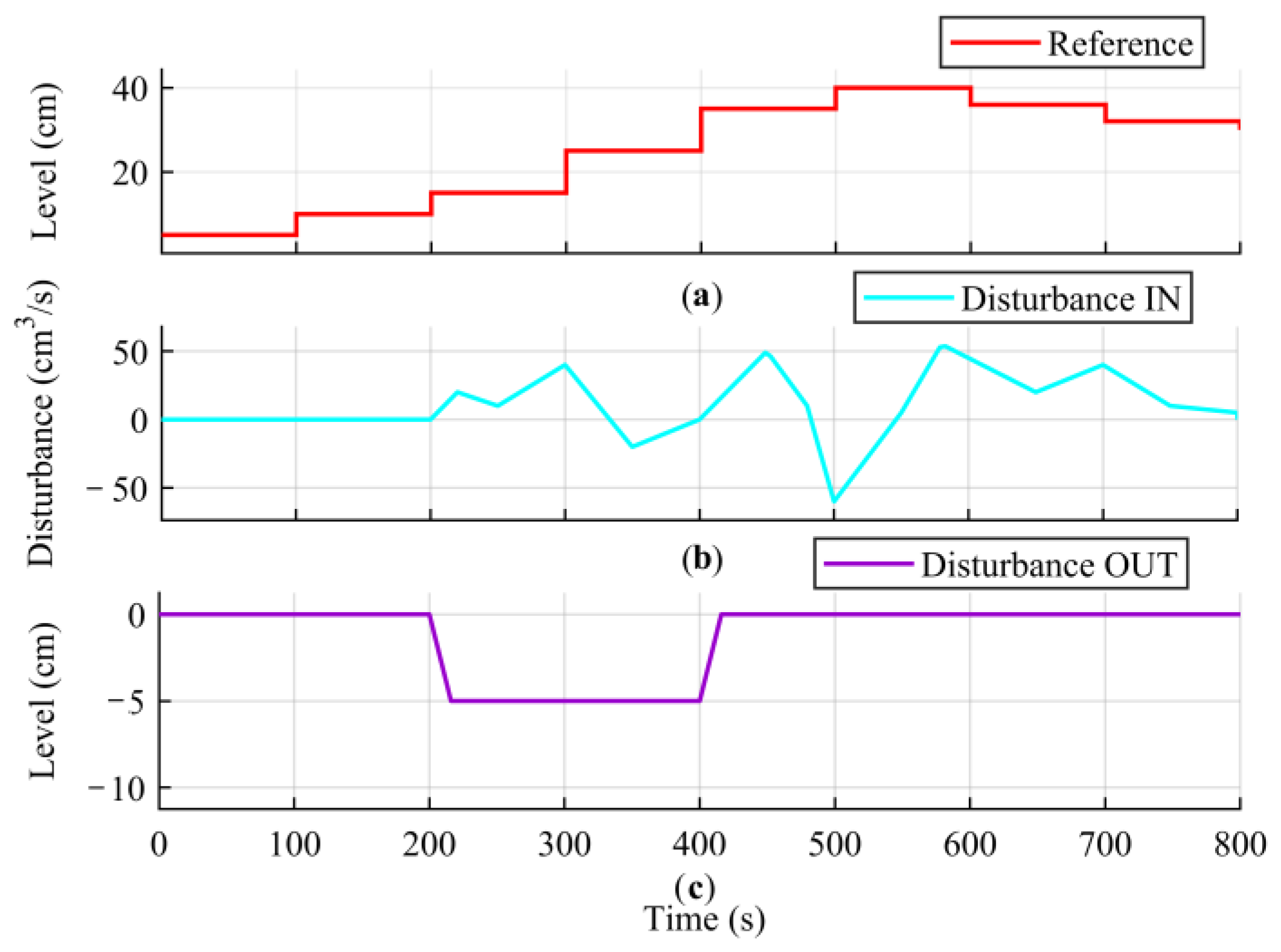
Figure 13 shows the test signals applied to verify the performance of the controllers designed. The signal represented in Figure 13a is a variable reference applied to the system input, with values from 5 to 40 cm. The signals in Figure 13b,c represent perturbations introduced both at the input and output of the system, respectively, for a constant reference value. Additionally, Figure 13b shows a random signal of ±50 cm3/s amplitude, while Figure 13c presents a transitory load disturbance.
4.1. Monitoring of Liquid Level Reference
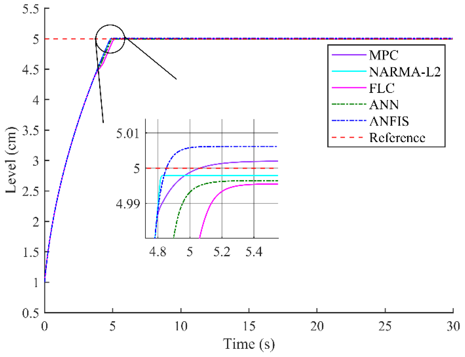
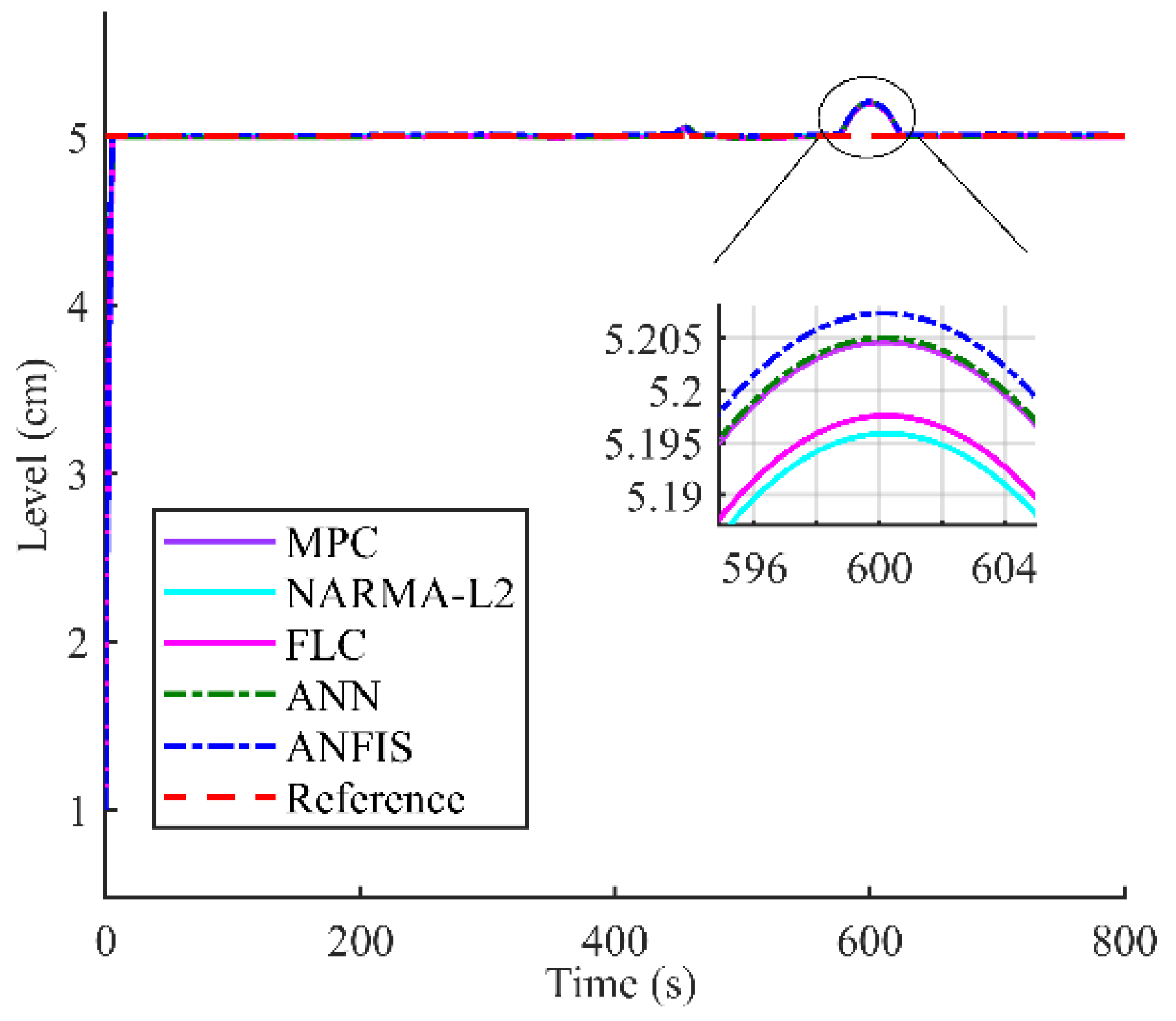
To observe the behavior of the controllers designed to monitor the liquid level reference, two tests were conducted. First, a fixed value of 5 cm was assigned and the behavior towards the variable reference value shown in Figure 13a was analyzed. Figure 14 shows the results obtained by five controllers designed for controlling the liquid level of a spherical tank whose reference value was set at a 5 cm.
Table 6 allows for a more precise analysis of the behavior of the control strategies by verifying their transient response. A set value of 2% is therefore considered for the level (cm) reached in a stable state (SS. Level), the maximum liquid level (Max. Level), Rise time (Tr), Settling time (Ts) and Overshoot.
As observed, all controllers reach the reference value quickly (about 5 s) and remain in a steady state. In this analysis, no significant differences were reported in their operation and an excellent transient response was obtained. To enrich the analysis, the PIs were calculated based on the error in the monitoring of the reference value. The PIs calculated for 10 s of simulation are shown in Table 7. Based on these values, the MPC and NARMA-L2 controllers present inferior PIs in all scenarios.
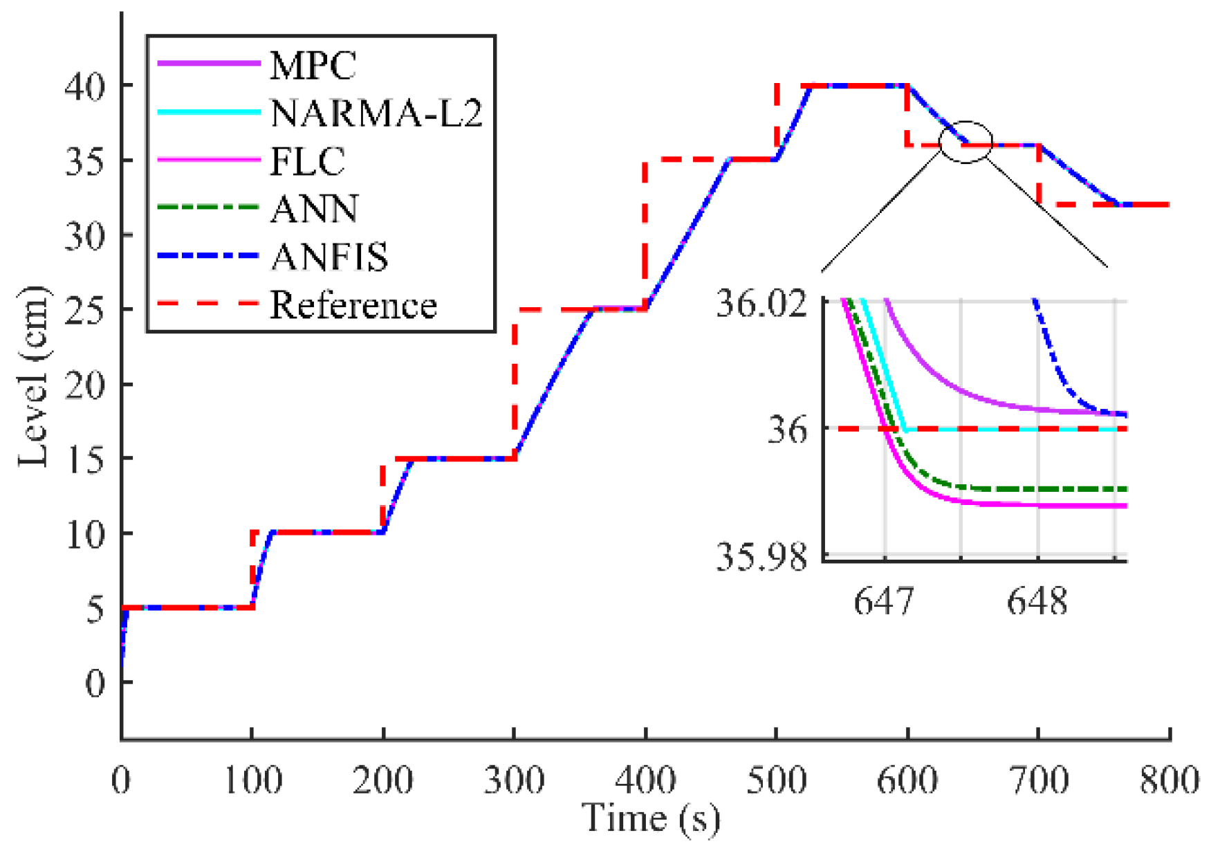
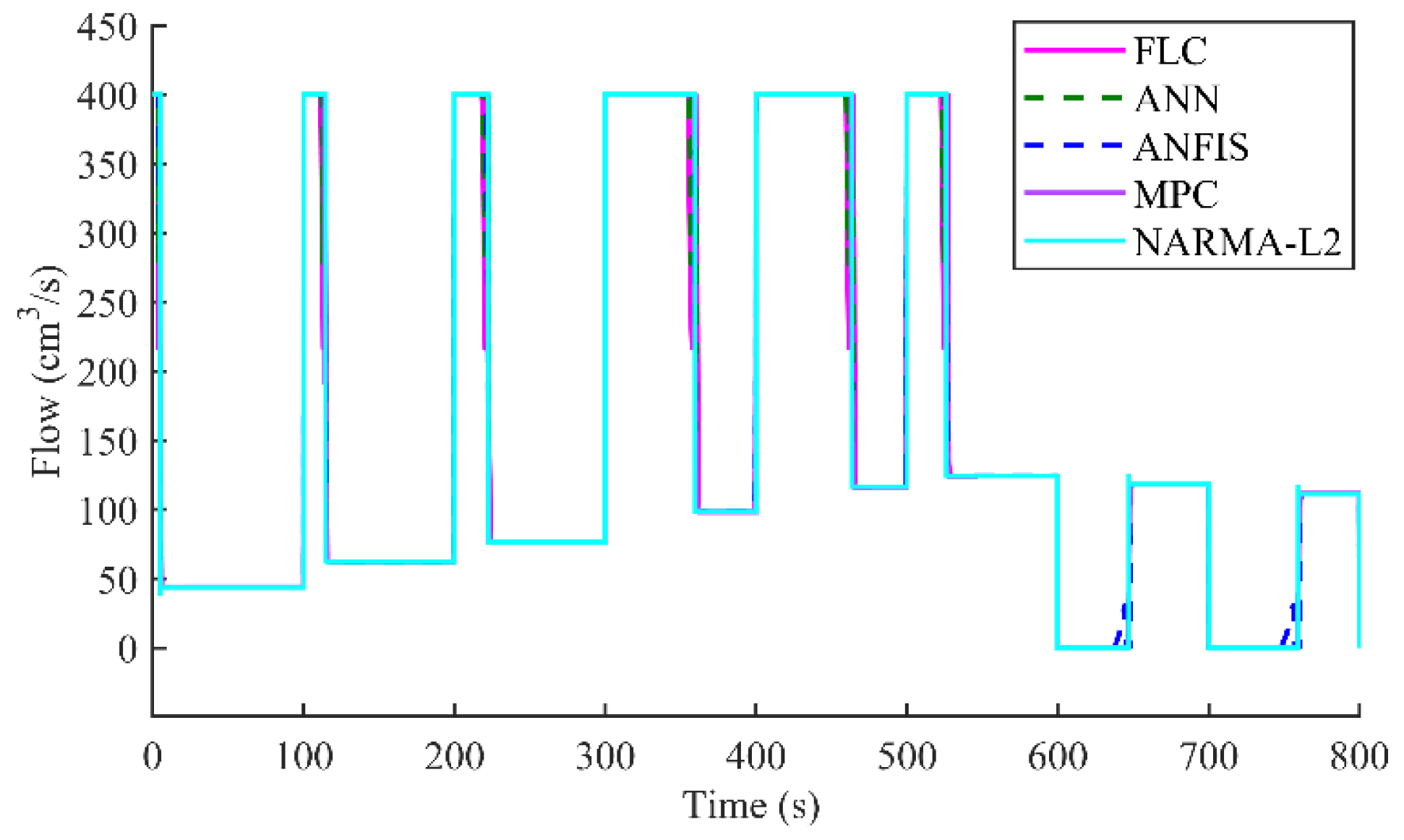
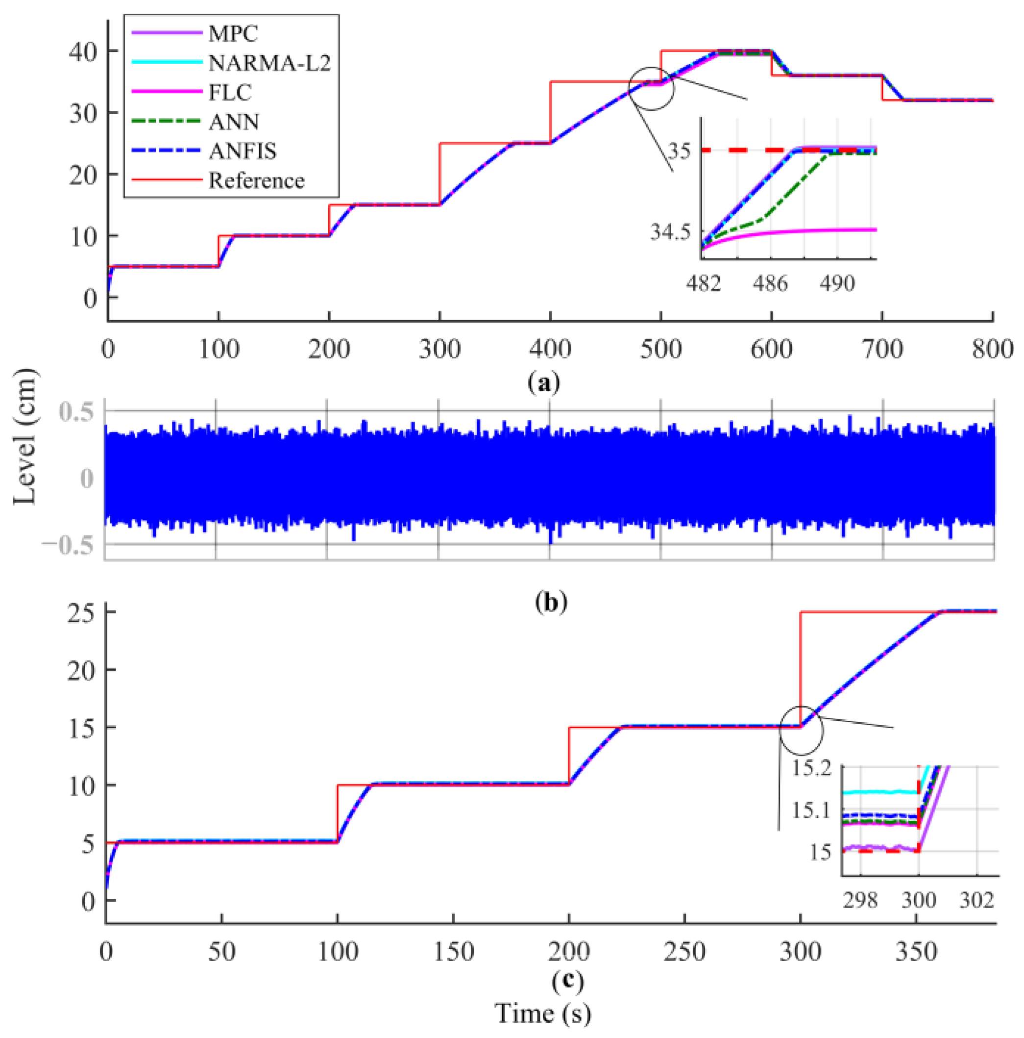
Figure 15 shows the results of liquid level control for a variable reference value and Figure 16 presents the control signal applied, which behaves correctly and within the established physical limits. As can be seen, all controllers stabilize the required liquid content readily, primarily during small increases of around 5 cm, in approximately 5 s. For liquid level increases of 5 cm, settling time increases; this is also the case when the liquid level of the deposit decreases, with an approximated settling time of 50 s.
Looking closer at the graph, it is noteworthy that the NARMA-L2 controller reaches the exact reference value in a shorter time than the other controllers. Nevertheless, each allows for reaching a liquid level very close to the reference value and in a short time. As such, the liquid level of the tank is controlled correctly in all scenarios.
4.2. Disturbance Rejection
When a disturbance occurs in the input of the system, the control of liquid level is affected in each of the controllers designed, which is normal. In this sense, the effort made by each of them to maintain the reference value and the time to achieve this need to be assessed. Figure 17 shows the result of liquid level control in the face of a disturbance at the input, like the one shown in Figure 13b.
As observed, all controllers minimize the effects of the disturbance, and this process is mostly affected when the input flow increases around 50 cm3/s. In this case, the graph shows that the controllers that minimize the disturbance more efficiently are NARMA-L2 and ANN, while ANFIS is the most affected. Table 8 presents the PIs calculated for this scenario in a time of 800 s. This confirms the best performance of the NARMA-L2 controller, primarily in terms of IAE and ITAE, indicating a fast system response as well as the minimization of error over time.
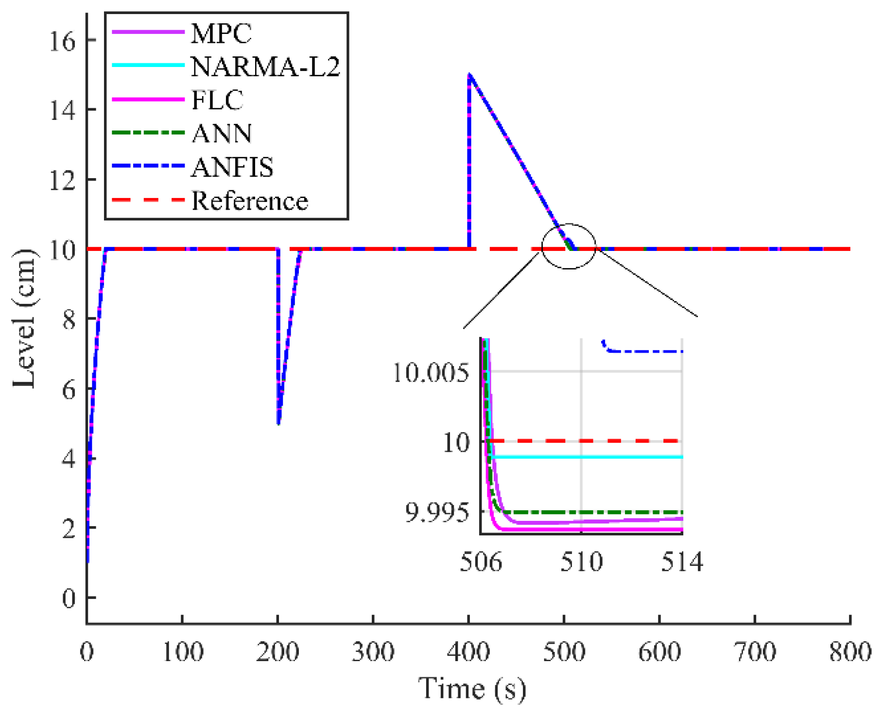
Figure 18 presents controller performance in the event of transitory load disturbance. As can be seen, all controllers adequately minimized the adverse effect of the disturbance, ultimately reaching the set reference value. As in the previous cases, the NARMA-L2 controller allows for a value closer to the reference value. However, in all scenarios, liquid level is stabilized at the desired height with a stationary state error below 0.01. As such, all the controllers are effective in all cases.
The results obtained when calculating PIs at an 800 s time frame are shown in Table 9. The best results for ISE and ITSE are achieved with ANN, indicating a rapid reduction in error by this controller. In turn, the best results for IAE and ITAE are reached with the NARMA-L2 controller, which points to a good transient response. Despite this distinction, in general, all controllers perform well.
4.3. Response of the System to Noise and Parametric Uncertainties
To analyze the robustness of the control techniques, several tests were conducted by subjecting the system to noise signals and parametric uncertainty. All tests were performed using the reference variable. The tests conducted were as follows:
The behavior of the control techniques was verified using the partial knowledge of the valve coefficient value. To this end, this parameter was varied between 9.69 and 69.69 cm2/s in increments of 10 cm2/s. The behavior of the controllers in the face of parametric uncertainty is shown in Figure 19a.
The effect of noise on the system was analyzed. For this calculation, the Band-Limited White Noise block from Simulink was used, which generates a normal distribution of random numbers with values within a range of approximately 10% of the input. The signal used is shown in Figure 19b. The error signal was added to the output of the plant, which can simulate damage to the sensor, or the effect of waves caused by the flow input to the plant, as shown in Figure 19c.
The parametric uncertainty analysis shows that the most affected controllers were FLC and ANN, both of which had difficulties following the reference. Noise caused the worst damage in controller operation, which was observed in commutations across all control signals. This effect causes significant damage to actuators, and therefore alternatives for attenuating its effect should be assessed. The MPC controller achieved an adequate tracking of the reference value, while NARMA-L2 became more distant from the desired value, which is reflected in a stationary state error.
4.4. Stability Analysis
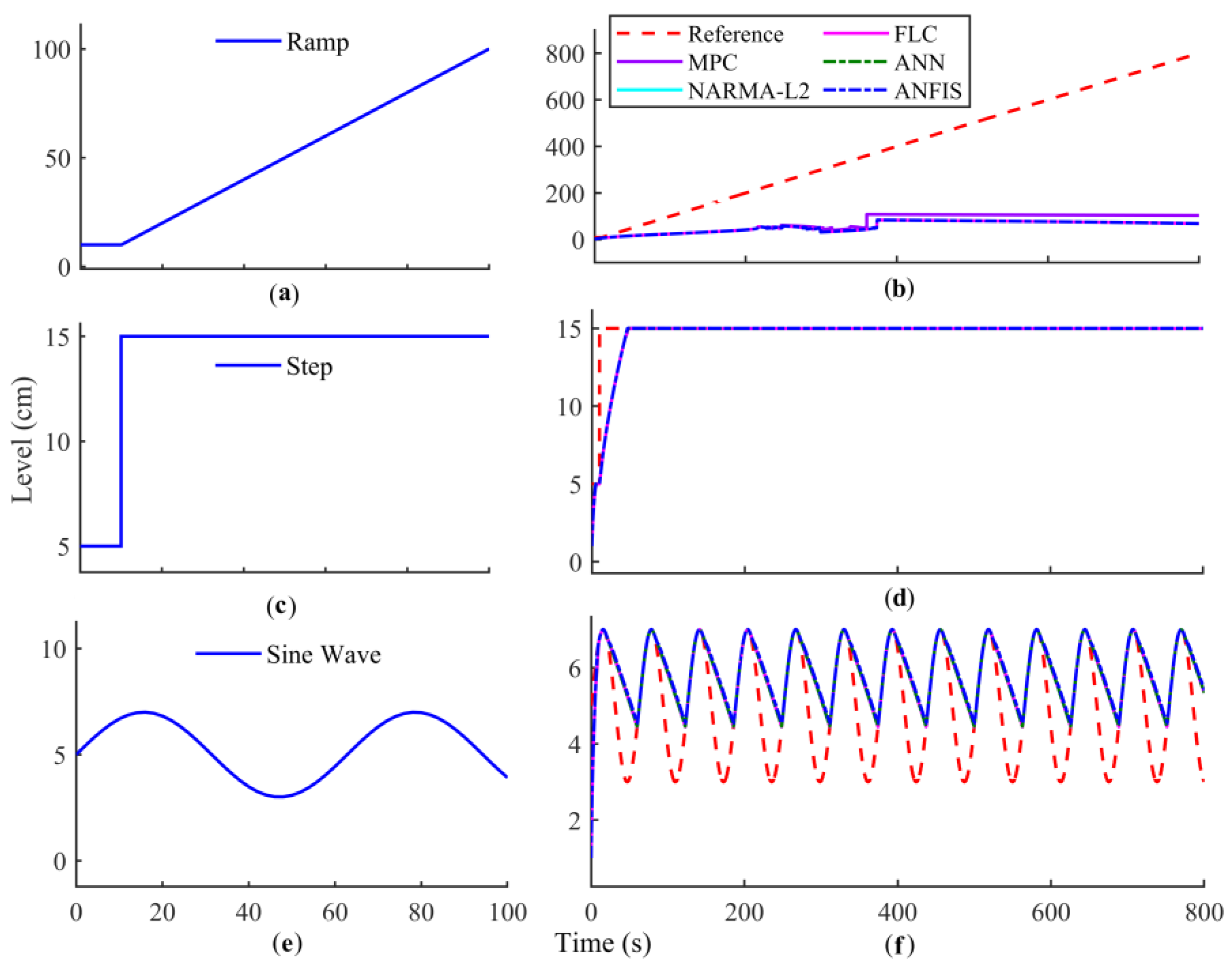
The stability analysis in linear systems has well-established standards, such as Routh–Hurwitz and Nyquist criteria. In nonlinear systems, this process is more complex, and techniques based on Lyapunov theory are employed. In the case of fuzzy and neural systems, the stability analysis exhibits peculiarities due to its complexity, despite the existence of Lyapunov analyses focused on them. In linear systems, when the behavior of the output signal is related to input signals, reference can be made to BIBO stability (Bounded-input, Bounded-output), among other criteria. BIBO stability establishes that the forced response of a stable linear system is constrained if its input is constrained. In general, it can be asserted that this rule is valid both for linear systems and nonlinear systems, which is considered in stability concepts such as Input-to-State Stability (ISS) [53].
Based on this, a stability analysis of the system in closed-loop is conducted graphically by applying several signals at the plant input. Figure 20 shows some of the signals used.
Figure 20a,c,e reflect the input signals applied to the system, while Figure 20b,d,f represent the response to the closed-loop. As observed, in the face of a constrained input signal, a constrained output signal is obtained, whereas when a non-constrained signal is applied, such as the ramp, the system reaches stability at some point. Therefore, this experiment may indicate that the closed-loop system presents stability.
In Table 10, a comparison is made between the results obtained by the designed controllers, specifically NARMA-L2, and the controllers reported by other authors for a spherical tank system. The parameters of the proposed method are determined for a 15-cm Set Point (SP). To establish a comparison in this case is complex, since despite the similarity of the system in terms of dimension, several aspects must be considered. These aspects include whether the plant model is linear or nonlinear, the type and quantity of tanks forming the system, simulation time and SP value.
In this case, all studies compared with the proposed method employ a transfer function, which implies better results in terms of transient characteristics and PIs. However, NARMA-L2 is observed to excel in some parameters analyzed, such as IAE and ITAE, when compared to [54], and settling time and IAE when compared to [2], without presenting overshoot. To establish a more accurate comparison, the fuzzy controller designed for a nonlinear conical tank system proposed in [7] is employed since the plants are similar. As observed, in addition to differences inherent to the analyzed plants, the parameters compared are similar, especially the absence of overshoot in the proposed method. In general, the results obtained are competitive with respect to the proposals of other authors and even imply better performance when using the linear model of the system.
5. Conclusions
In this study, five strategies for controlling the liquid level contained in a spherical tank were developed. To this end, several criteria were established, such as maximum and minimum flow at the input of the system, in order to enhance the applicability of the study results. Additionally, the response of the controllers to diverse scenarios that could occur during an industrial process was assessed.
The designed controllers showed excellent transient response, with a rise time of less than 4 s and settling times of approximately 5 s for a 5-cm level; for a 10-cm level, settling time is around 20 s. No overshooting or oscillations were observed during reference tracking. In turn, error-based performance indices allowed for an adequate analysis of the performance of the control strategies assessed.
While conducting this study, it was considered that the signal control did not exceed an input flow with a maximum value of 400 cm3/s and a minimum value of 0 cm3/s; this is a fundamental design criterion. Because of these pre-set flow limits, a natural effort is observed from the controllers to stabilize the fluid contained in the tank in the event of increases or decreases. It is observed that, primarily when liquid decreases, the process occurs lightly in a time slightly over 100 s. If these limit values for flow had not been considered, better results would have been obtained for both the graphic responses of controllers and their corresponding PIs. However, such results would have been far from the real behavior of each controller.
In the case of the MPC controller, obtaining the plant linearized model was more efficient through optimization methods. This controller, despite being affected by noise, was the best at reference tracking. Conversely, the FLC controller showed the worst performance in reference tracking despite being good overall. However, although this controller has the main advantage of not requiring knowledge of the plant model, deep knowledge of its operation is necessary. In addition, FLC does not usually show stability problems and is widely employed in tank systems and industrial processes.
The NARMA-L2 controller obtained the best results in most of the comparison parameters established. Considering the results obtained, it could be said that, as with all methods based on machine learning, the quality and quantity of the training data improves controller performance. For the NARMA-L2 controller, the identification of the plant was conducted by applying random signals, and a greater number of samples were collected than in the rest of the controllers when some type of learning was applied; this is considered to have been determinant in the results obtained. It is worth noting that, in the NARMA-L2 control signal, the occurrence of oscillations was observed.
In turn, controllers designed based on neural networks essentially depend on training data for good behavior. To this end, it is useful to select adequate signals according to the system under study. Some useful signals may be sinusoidal, pseudo-random or noise-type, among others. The selection of hidden layers or of the number of neurons in them may depend on the experience of the developer and this is often determined experimentally.
The FLC and ANN controllers showed a more discrete performance, being affected to a greater extent by disturbances, noise and parametric uncertainties. Additionally, the ANFIS, MPC and NARMA-L2 controllers exhibited a competitive performance. In all cases, the stability of the closed-loop system was verified. It should be noted, as a negative aspect, that all controllers were strongly affected by the noise simulated in the sensor. This problem could be minimized by the use of carefully selected filters based on noise type. However, this procedure could cause undesired effects, which makes it an interesting aspect to address in future research.
Future research should focus on applying other primarily data-based control techniques to the system under study. The need for mathematical modeling of the plant often becomes a limitation that significantly affects the performance of controllers that require it. Therefore, it is important to develop control strategies that are independent from knowledge of the same. The implementation of data-based controllers is a promising option as it allows for the design of control strategies in complex systems, namely nonlinear systems, systems with unknown dynamics, unforeseeable disturbance, high dimensionality and other factors that affect real processes. Furthermore, considering the good performance of the controllers proposed in this article, assessing their performance in more complex systems should be considered, such as with surgical robots, as, in their field, smart control techniques are fundamental and research has focused on contributing some degree of autonomy.
Author Contributions
Conceptualization, C.U. and Y.G.-G.; Methodology, C.U. and Y.G.-G.; Software, C.U. and Y.G.-G.; Validation, C.U. and Y.G.-G.; Formal analysis, C.U. and Y.G.-G.; Investigation, C.U. and Y.G.-G.; Resources, C.U. and Y.G.-G.; Data curation, C.U. and Y.G.-G.; Writing—original draft preparation, C.U. and Y.G.-G.; Writing—review and editing, C.U.; Visualization, C.U. and Y.G.-G.; Supervision, C.U.; Project administration, C.U.; Funding acquisition, C.U. All authors have read and agreed to the published version of the manuscript.
Funding
This research received no external funding.
Data Availability Statement
Not applicable.
Acknowledgments
This work was supported by the Faculty of Engineering of the University of Santiago of Chile, Chile.
Conflicts of Interest
The authors declare no conflict of interest.
References
- Sreepradha, C.; Deepa, P.; Panda, R.C.; Manamali, M.; Shivakumar, R. Synthesis of fuzzy sliding mode controller for liquid level control in spherical. Cogent Eng. 2016, 3, 1222042. [Google Scholar] [CrossRef]
- Priya, C.; Lakshmi, P. Particle swarm optimisation applied to real time control of spherical tank system. Int. J. Bio-Inspired Comput. 2012, 4, 206–216. [Google Scholar] [CrossRef]
- Zheng, W.; Wang, H.B.; Wen, S.H.; Wang, H.R.; Zhang, Z.M. Adaptive dynamic output-feedback control for chemical continuous stirred tank reactor system with nonlinear uncertainties and multiple time-delays. Int. J. Control Autom. Syst. 2018, 16, 1681–1691. [Google Scholar] [CrossRef]
- Hosen, M.A.; Khosravi, A.; Kabir, H.D.; Johnstone, M.; Creighton, D.; Nahavandi, S.; Shi, P. NN-based Prediction Interval for Nonlinear Processes Controller. Int. J. Control Autom. Syst. 2021, 19, 3239–3252. [Google Scholar] [CrossRef]
- Zheng, W.; Zhang, Z.M.; Wang, H.B.; Wang, H.R.; Yin, P.H. Stability analysis and dynamic output feedback control for nonlinear TS fuzzy system with multiple subsystems and normalized membership functions. Int. J. Control Autom. Syst. 2018, 16, 2801–2813. [Google Scholar] [CrossRef]
- Yu, S.; Lu, X.; Zhou, Y.; Feng, Y.; Qu, T.; Chen, H. Liquid level tracking control of three-tank systems. Int. J. Control Autom. Syst. 2020, 18, 2630–2640. [Google Scholar] [CrossRef]
- Urrea, C.; Páez, F. Design and Comparison of Strategies for Level Control in a Nonlinear Tank. Processes 2021, 9, 735. [Google Scholar] [CrossRef]
- Mahmood, Q.A.; Nawaf, A.T.; Mohamedali, S.A. Simulation and performance of liquid level controllers for linear tank. J. Teknol. 2020, 82, 75–82. [Google Scholar] [CrossRef]
- Saxena, A.; Dubey, Y.; Kumar, M.; Saxena, A. Performance Comparison of ANFIS, FOPID-PSO and FOPID-Fuzzy Tuning Methodology for Optimizing Response of High-Performance Drilling Machine. IETE J. Res. 2021, 1–14. [Google Scholar] [CrossRef]
- Jegatheesh, A.; Kumar, C.A. Novel fuzzy fractional order PID controller for nonlinear interacting coupled spherical tank system for level process. Microprocess. Microsyst. 2020, 72, 102948. [Google Scholar] [CrossRef]
- Mehri, E.; Tabatabaei, M. Control of Quadruple Tank Process Using an Adaptive Fractional-Order Sliding Mode Controller. J. Control Autom. Electr. Syst. 2021, 32, 605–614. [Google Scholar] [CrossRef]
- Ayten, K.K.; Dumlu, A. Implementation of a PID type Sliding-Mode Controller Design based on Fractional Order Calculus for Industrial Process System. Elektron. IR Elektrotechnika 2021, 27, 4–10. [Google Scholar] [CrossRef]
- Rajesh, R. Optimal tuning of FOPID controller based on PSO algorithm with reference model for a single conical tank system. SN Appl. Sci. 2019, 1, 758. [Google Scholar] [CrossRef] [Green Version]
- Ardjal, A.; Bettayeb, M.; Mansouri, R.; Zouak, B. Design and implementation of a model-free fractional order intelligent PI fractional order sliding mode controller for water level tank system. ISA Trans. 2022, 127, 501–510. [Google Scholar] [CrossRef] [PubMed]
- Choueikh, S.; Kermani, M.; M’sahli, F. A Comparative Study of Nonsingular Terminal Sliding Mode and Backstepping Schemes for the Coupled Two-Tank System. Complexity 2021, 2021, 5546535. [Google Scholar] [CrossRef]
- Pham, T.T.; Nguyen, C.-N. Adaptive Fuzzy Proportional Integral Sliding Mode Control for Two-Tank Interacting System. J. Eng. Technol. Sci. 2022, 54, 220310. [Google Scholar] [CrossRef]
- Bagyaveereswaran, V.; Arulmozhivarman, P. Gain scheduling of a robust setpoint tracking disturbance rejection and aggressiveness controller for a nonlinear process. Processes 2019, 7, 415. [Google Scholar] [CrossRef] [Green Version]
- Xu, Z.; Fan, Q.; Zhao, J. Gain-Scheduled Equivalent-Cascade IMC Tuning Method for Water Level Control System of Nuclear Steam Generator. Processes 2020, 8, 1160. [Google Scholar] [CrossRef]
- Meng, X.; Yu, H.; Xu, T.; Wu, H. Disturbance Observer and L 2-Gain-Based State Error Feedback Linearization Control for the Quadruple-Tank Liquid-Level. System. Energies 2020, 13, 5500. [Google Scholar] [CrossRef]
- Meng, X.; Yu, H.; Zhang, J.; Yan, K. Optimized control strategy based on EPCH and DBMP algorithms for quadruple-tank liquid level system. J. Process Control 2022, 110, 121–132. [Google Scholar] [CrossRef]
- Torga, D.S.; da Silva, M.T.; Reis, L.A.; Euzébio, T.A. Simultaneous tuning of cascade controllers based on nonlinear optimization. Trans. Inst. Meas. Control 2022, 44, 3118–3131. [Google Scholar] [CrossRef]
- Patil, N.A.; Lakhekar, G.V. Design of PID controller for cascade control process using genetic algorithm. In Proceedings of the 2017 International Conference on Intelligent Computing and Control Systems (ICICCS), Madurai, India, 15–16 June 2017; pp. 1089–1095. [Google Scholar] [CrossRef]
- Somkane, P.; Kongratana, V.; Gulpanich, S.; Tipsuwanporn, V.; Wongvanich, N. A study of flow-level cascade control with WirelessHART TM transmitter using LabVIEW. In Proceedings of the 2017 17th International Conference on Control, Automation and Systems (ICCAS 2017), Ramada Plaza, Jeju, Republic of Korea, 18–21 October 2017; pp. 856–861. [Google Scholar]
- Mohan, V.; Pachauri, N.; Panjwani, B.; Kamath, D.V. A novel cascaded fractional fuzzy approach for control of fermentation process. Bioresour. Technol. 2022, 357, 127377. [Google Scholar] [CrossRef]
- Kaya, İ.; Nalbantoğlu, M. Simultaneous tuning of cascaded controller design using genetic algorithm. Electr. Eng. 2016, 98, 299–305. [Google Scholar] [CrossRef]
- Lyden, A.; Tuohy, P.G. Planning level sizing of heat pumps and hot water tanks incorporating model predictive control and future electricity tariffs. Energy 2022, 238, 121731. [Google Scholar] [CrossRef]
- Jakowluk, W.; Jaszczak, S. Cascade tanks system identification for robust predictive control. Bull. Pol. Acad. Sci. Tech. Sci. 2022, 70, e143646. [Google Scholar] [CrossRef]
- Kang, T.; Peng, H.; Zhou, F.; Tian, X.; Peng, X. Robust predictive control of coupled water tank plant. Appl. Intell. 2021, 51, 5726–5744. [Google Scholar] [CrossRef]
- Júnior, M.P.; da Silva, M.T.; Guimarães, F.G.; Euzébio, T.A. Energy savings in a rotary dryer due to a fuzzy multivariable control application. Dry. Technol. 2020, 40, 1196–1209. [Google Scholar] [CrossRef]
- Lott, G.D.; da Silva, M.T.; Cota, L.P.; Guimarães, F.G.; Euzébio, T.A. Fuzzy Decision Support System for the Calibration of Laboratory-Scale Mill Press Parameters. IEEE Access 2021, 9, 24901–24912. [Google Scholar] [CrossRef]
- Vasconcelos, F.J.D.S.; Medeiros, C.M.D.S. Performance comparison between PI digital and fuzzy controllers in a level control system. J. Mechatron. Eng. 2019, 2, 10–18. [Google Scholar] [CrossRef] [Green Version]
- Aslan, Ö.; Altan, A.; Hacıoğlu, R. Level Control of Blast Furnace Gas Cleaning Tank System with Fuzzy Based Gain Regulation for Model Reference Adaptive Controller. Processes 2022, 10, 2503. [Google Scholar] [CrossRef]
- Pandian, B.J.; Noel, M.M. Control of constrained high dimensional nonlinear liquid level processes using a novel neural network based Rapidly exploring Random Tree algorithm. Appl. Soft Comput. 2020, 96, 106709. [Google Scholar] [CrossRef]
- Antão, R.; Antunes, J.; Mota, V.; Escadas Martins, R. Model Predictive Control of Non-Linear Systems Using Tensor Flow-Based Models. Appl. Sci. 2020, 10, 3958. [Google Scholar] [CrossRef]
- Çetin, M.; Bahtiyar, B.; Beyhan, S. Adaptive uncertainty compensation-based nonlinear model predictive control with real-time applications. Neural Comput. Applic. 2019, 31, 1029–1043. [Google Scholar] [CrossRef]
- Jones, D.M.; Kanagalakshmi, S. Data Driven Control of Interacting Two Tank Hybrid System using Deep Reinforcement Learning. In Proceedings of the Name of the 2021 IEEE 6th International Conference on Computing, Communication and Automation (ICCCA), Arad, Romania, 17–19 December 2021. [Google Scholar] [CrossRef]
- Jeyaraj, P.R.; Nadar, E.R.S. Real-time data-driven PID controller for multivariable process employing deep neural network. Asian J. Control 2022, 24, 3240–3251. [Google Scholar] [CrossRef]
- Munoz, S.A.; Park, J.; Stewart, C.M.; Hedengren, J.D. Deep Transfer Learning for Approximate Model Predictive Control. Processes 2023, 11, 197. [Google Scholar] [CrossRef]
- Mary, A.H. ANFIS Based Reinforcement Learning Strategy for Control A Nonlinear Coupled Tanks System. J. Electr. Eng. Technol. 2021, 17, 1921–1929. [Google Scholar] [CrossRef]
- Rose, T.P.; Devadhas, G.G. Detection of pH neutralization technique in multiple tanks using ANFIS controller. Microprocess. Microsyst. 2020, 72, 102845. [Google Scholar] [CrossRef]
- Uçak, K.; Günel, G.Ö. Online Support Vector Regression Based Adaptive NARMA-L2 Controller for Nonlinear Systems. Neural Process Lett. 2021, 53, 405–428. [Google Scholar] [CrossRef]
- Bachi, I.O.; Bahedh, A.S.; Kheioon, I.A. Design of control system for steel strip-rolling mill using NARMA-L2. J. Mech. Sci. Technol. 2021, 35, 1429–1436. [Google Scholar] [CrossRef]
- Jibril, M.; Tadese, M.; Alemayehu, E. Tank liquid level control using NARMA-L2 and MPC controllers. ScienceOpen Prepr. 2020, 12, 23–27. [Google Scholar] [CrossRef]
- Krishnapriya, K.; Devi, M.R.; Roshini, U.; Jayachitra, A. Analyzing the performance of interacting spherical tank system using internal model controller (IMC) and Metaheurstic algorithm. Int. J. Adv. Res. Comput. Commun. Eng. 2017, 6, 36–42. [Google Scholar]
- Jegatheesh, A.; Nisha, M.; Kopperundevi, N. A Novel ANFIS Based SMC with Fractional Order PID Controller. Intell. Autom. Soft Comput. 2023, 36, 745–760. [Google Scholar] [CrossRef]
- Fogarty, P. Fuzzy Logic, a Logician’s Perspective. In Fuzzy Logic: Recent Applications and Developments; Carter, J., Chiclana, F., Khuman, A.S., Chen, T., Eds.; Springer Nature: Cham, Switzerland, 2021; pp. 1–10. [Google Scholar] [CrossRef]
- Vishnoi, V.; Tiwari, S.; Singla, R.K. Controller Design for Temperature Control of MISO Water Tank System: Simulation Studies. Int. J. Cogn. Inform. Nat. Intell. 2021, 15, 1–13. [Google Scholar] [CrossRef]
- Sharma, S.; Obaid, A.J. Mathematical modelling, analysis and design of fuzzy logic controller for the control of ventilation systems using MATLAB fuzzy logic toolbox. J. Interdiscip. Math. 2020, 23, 843–849. [Google Scholar] [CrossRef]
- MathWorks MatLab Documentation. Available online: https://www.mathworks.com/ (accessed on 10 January 2023).
- Laughton, M.A.; Warne, D.J. Electrical Engineer’s Reference Book, 16th ed.; Elsevier Science: Amsterdam, The Netherlands, 2003; pp. 13–44. [Google Scholar]
- Slotine, J.-J.E.; Li, W. Applied Nonlinear Control; Prentice-Hall: Englewood Cliffs, NJ, USA, 1991; ISBN 0-130-40890-5. [Google Scholar]
- Urrea, C.; Venegas, D. Design and development of control systems for an aircraft. Comparison of performances through computational simulations. IEEE Lat. Am. Trans. 2018, 16, 735–740. [Google Scholar] [CrossRef]
- Gordillo, F. Estabilidad de sistemas no lineales basada en la teoría de Liapunov. Rev. Iberoam. Automática Inf. Ind. (RIAI) 2009, 6, 5–16. [Google Scholar] [CrossRef] [Green Version]
- Govind, K.R.A.; Mahapatra, S. Frequency Domain Specifications Based Robust Decentralized PI/PID Control Algorithm for Benchmark Variable-Area Coupled Tank Systems. Sensors 2022, 22, 9165. [Google Scholar] [CrossRef]
Figure 1.
Applications of MPC, FLC, ANN, ANFIS and NARMA-L2 controllers.

Figure 2.
Physical diagram of the spherical tank system.

Figure 3.
Fuzzy controller designed. (a) Diagram of FLC controller. (b) Block diagram of implementation in Simulink.
Figure 3.
Fuzzy controller designed. (a) Diagram of FLC controller. (b) Block diagram of implementation in Simulink.

Figure 4.
Membership functions for error.

Figure 5.
Membership functions for derivative of the error.

Figure 6.
Membership functions for output.

Figure 7.
Artificial Neural Network architecture. (a) Diagram of ANN controller; 2 inputs and 1 output are defined, 9 neurons were assigned in the hidden layer and 1 in the output layer, where w represents the weights and b the bias. (b) Block diagram of implementation in Simulink.
Figure 7.
Artificial Neural Network architecture. (a) Diagram of ANN controller; 2 inputs and 1 output are defined, 9 neurons were assigned in the hidden layer and 1 in the output layer, where w represents the weights and b the bias. (b) Block diagram of implementation in Simulink.


Figure 8.
ANFIS architecture. (a) Diagram of the ANFIS controller. (b) Block diagram of the implementation in Simulink.
Figure 8.
ANFIS architecture. (a) Diagram of the ANFIS controller. (b) Block diagram of the implementation in Simulink.

Figure 9.
Performance comparison of different MFs.

Figure 10.
Membership functions at the input of ANFIS.

Figure 11.
MPC architecture. (a) Diagram of MPC controller. (b) Block diagram of implementation in Simulink.
Figure 11.
MPC architecture. (a) Diagram of MPC controller. (b) Block diagram of implementation in Simulink.


Figure 12.
NARMA-L2 architecture. (a) Block diagram of the NARMA-L2 controller [49]. (b) Block diagram of implementation in Simulink.
Figure 12.
NARMA-L2 architecture. (a) Block diagram of the NARMA-L2 controller [49]. (b) Block diagram of implementation in Simulink.

Figure 13.
Test signals for verifying the performance of the controllers. (a) Variable reference. (b) Perturbation introduced at the input of the system (supply disturbances). (c) Perturbation introduced at the output of the system (load disturbances).
Figure 13.
Test signals for verifying the performance of the controllers. (a) Variable reference. (b) Perturbation introduced at the input of the system (supply disturbances). (c) Perturbation introduced at the output of the system (load disturbances).

Figure 14.
Result of liquid level control in the spherical tank compared to the fixed reference value.
Figure 14.
Result of liquid level control in the spherical tank compared to the fixed reference value.

Figure 15.
Results of liquid level control in the spherical tank compared to the variable reference value.
Figure 15.
Results of liquid level control in the spherical tank compared to the variable reference value.

Figure 16.
Control signal employed for monitoring the reference variable.

Figure 17.
Result of liquid level control in the spherical tank under a disturbance at the system input.
Figure 17.
Result of liquid level control in the spherical tank under a disturbance at the system input.

Figure 18.
Result of liquid level control in the spherical tank under a transitory load disturbance.
Figure 18.
Result of liquid level control in the spherical tank under a transitory load disturbance.

Figure 19.
Controller performance in the face of parametric uncertainty and noise. (a) Control response to parametric uncertainty. (b) Noise signal used. (c) Effects of noise on process control.
Figure 19.
Controller performance in the face of parametric uncertainty and noise. (a) Control response to parametric uncertainty. (b) Noise signal used. (c) Effects of noise on process control.

Figure 20.
Response of closed-loop system to diverse input signals. (a) Ramp signal. (b) Response of the system to the ramp signal. (c) Step signal. (d) Response of the system to the step signal. (e) Sinusoidal signal. (f) Response of the system to the sinusoidal signal.
Figure 20.
Response of closed-loop system to diverse input signals. (a) Ramp signal. (b) Response of the system to the ramp signal. (c) Step signal. (d) Response of the system to the step signal. (e) Sinusoidal signal. (f) Response of the system to the sinusoidal signal.


| Variable | Symbol | Values |
|---|---|---|
| Tank radius | R | 25 cm |
| Tank height | H | 50 cm |
| Tank liquid level (controlled variable) | h | cm |
| Valve coefficient | β | 19.69 cm2/s |
| Input flow (manipulated variable) | Fin(t) | cm3/s |
| Output flow | Fout(t) | cm3/s |
| Flow (auxiliary output) | FL(t) | cm3/s |
Table 2.
Inference rule bases for FLC.
| e(t) | NB | NM | NS | Z | PS | PM | PB |
|---|---|---|---|---|---|---|---|
| de/dt | |||||||
| deNB | CB | CB | CB | O | OB | OS | OB |
| deNM | CB | CB | CB | O | OB | OS | OB |
| deNS | CB | CB | CB | O | OB | OS | OB |
| deZ | CB | CB | CB | O | OB | OS | OB |
| dePS | CB | CB | CB | O | OB | OS | OB |
| dePM | CB | CB | CB | O | OB | OS | OB |
| dePB | CB | CB | CB | O | OB | OS | OB |
Table 3.
Training error in ANFIS based on MFs.
| MFs | Error Based on Quantity of MFs | ||||
|---|---|---|---|---|---|
| 3 | 4 | 5 | 6 | 7 | |
| dsigmf | 19.28 | 18.16 | 15.43 | 14.87 | 12.58 |
| gaussmf | 20.52 | 19.08 | 17.57 | 15.57 | 15.49 |
| gauss2mf | 22.77 | 19.26 | 15.26 | 14.74 | 19.69 |
| gbellmf | 20.45 | 20.33 | 16.92 | 17.57 | 14.40 |
| pimf | 20.89 | 18.22 | 12.98 | 13.95 | 9.41 |
| psigmf | 19.29 | 18.16 | 15.31 | 14.87 | 12.56 |
| trapmf | 12.00 | 13.49 | 12.77 | 8.96 | 18.60 |
| trimf | 11.61 | 5.32 | 10.69 | 5.73 | 14.60 |
Table 4.
Design parameters for MPC controller.
| Horizon |
| Sample time (s): 0.001 |
| Control horizon: 5 |
| Prediction horizon: 20 |
| Constraints |
| Max. system input: 400 |
| Min. system input: 0 |
| Max. system output: 50 |
| Min. system output: 1 |
| Weights |
| Input weights: 0.001 |
| Rate weights: 0.1 |
| Output weights: 100 |
Table 5.
Design parameters for NARMA-L2.
| Network Architecture |
| Size of hidden layer: 9 |
| Sample interval (s): 0.001 |
| Delayed system input: 2 |
| Delayed system output: 2 |
| Training data |
| Max. system input: 400 |
| Min. system input: 0 |
| Max. system output: 50 |
| Min. system output: 1 |
| Min. interval value (s): 0.001 |
| Max. interval value (s): 0.005 |
| Training simple: 668,300 |
| Training parameters |
| Training epochs: 1000 |
| Training function: trainbr |
Table 6.
Transient response for a reference value of 5 cm.
| FLC | ANN | ANFIS | MPC | NARMA-L2 | |
|---|---|---|---|---|---|
| SS. Level (cm) | 4.996 | 4.997 | 5.008 | 5.002 | 4.998 |
| Max. Level (cm) | 4.996 | 4.997 | 5.008 | 5.002 | 4.998 |
| Tr (s) | 3.73 | 3.66 | 3.62 | 3.66 | 3.62 |
| Ts (s) | 5.06 | 4.90 | 4.78 | 4.90 | 4.78 |
| Overshoot (%) | 0 | 0 | 0 | 0 | 0 |
Table 7.
Performance indexes for fixed reference (5 cm).
| PIs | FLC | ANN | ANFIS | MPC | NARMA-L2 |
|---|---|---|---|---|---|
| ISE | 17.31 | 17.27 | 17.25 | 17.25 | 17.25 |
| ITSE | 17.66 | 17.48 | 17.40 | 17.39 | 17.39 |
| IAE | 7.68 | 7.60 | 7.56 | 7.54 | 7.54 |
| ITAE | 11.86 | 11.46 | 11.32 | 11.17 | 11.17 |
Table 8.
Performance indexes for a disturbance at the input of the spherical tank.
| PIs | FLC | ANN | ANFIS | MPC | NARMA-L2 |
|---|---|---|---|---|---|
| ISE | 18.19 | 17.96 | 18.39 | 18.37 | 18.24 |
| ITSE | 594.60 | 585.70 | 688.80 | 685.20 | 610.40 |
| IAE | 16.92 | 17.44 | 19.49 | 16.65 | 15.67 |
| ITAE | 4887 | 5172 | 6140 | 5095 | 4519 |
Table 9.
Performance indexes for transitory load disturbance.
| PIs | FLC | ANN | ANFIS | MPC | NARMA-L2 |
|---|---|---|---|---|---|
| ISE | 1366 | 1361 | 1381 | 1379 | 1377 |
| ITSE | 413,900 | 410,300 | 420,500 | 418,500 | 417,700 |
| IAE | 386.90 | 396.30 | 388.40 | 385.40 | 383.70 |
| ITAE | 128,800 | 134,000 | 130,500 | 128,400 | 127,800 |
Table 10.
Comparison between the performance of the controllers designed and results from other authors.
Table 10.
Comparison between the performance of the controllers designed and results from other authors.
| Controllers | SP (cm) | Time (s) | Comparison Criterion | |||||
|---|---|---|---|---|---|---|---|---|
| Ts (s) | Tr (s) | Overshoot (%) | ISE | IAE | ITAE | |||
| Fuzzy-based SMC [1] | 15 | 15 | -- | -- | -- | -- | 2.358 | -- |
| PSO-based PI [2] | 25 | 1000 | 290 | -- | 1.57 | 41.45 | 2255 | -- |
| ANFIS based SMC-FOPID [45] | Region1 | 800 | 1 × 10⁻⁶ | 0.003 | 0 | 2 | 0.1 | 2.587 × 10⁻¹⁶ |
| Robust decentralized PI/PID [54] | 15 (h1) | 500 | -- | -- | -- | 103.8 | 753.7 | 7088 |
| Fuzzy [7] | 35–45 | 90 | 14.40 | 14.00 | 6.40 | 647.10 | 107.90 | 1665 |
| Proposed method (NARMA-L2) | 5–15 | 100 | 36.37 | 29.43 | 0 | 956.20 | 157.10 | 1808 |
Disclaimer/Publisher’s Note: The statements, opinions and data contained in all publications are solely those of the individual author(s) and contributor(s) and not of MDPI and/or the editor(s). MDPI and/or the editor(s) disclaim responsibility for any injury to people or property resulting from any ideas, methods, instructions or products referred to in the content. |
© 2023 by the authors. Licensee MDPI, Basel, Switzerland. This article is an open access article distributed under the terms and conditions of the Creative Commons Attribution (CC BY) license (https://creativecommons.org/licenses/by/4.0/).
Share and Cite
MDPI and ACS Style
Urrea, C.; Garcia-Garcia, Y. Design and Performance Analysis of Level Control Strategies in a Nonlinear Spherical Tank. Processes 2023, 11, 720. https://doi.org/10.3390/pr11030720
AMA Style
Urrea C, Garcia-Garcia Y. Design and Performance Analysis of Level Control Strategies in a Nonlinear Spherical Tank. Processes. 2023; 11(3):720. https://doi.org/10.3390/pr11030720
Chicago/Turabian StyleUrrea, Claudio, and Yainet Garcia-Garcia. 2023. "Design and Performance Analysis of Level Control Strategies in a Nonlinear Spherical Tank" Processes 11, no. 3: 720. https://doi.org/10.3390/pr11030720
Note that from the first issue of 2016, this journal uses article numbers instead of page numbers. See further details here.