Efficient and Noise Robust Photon-Counting Imaging with First Signal Photon Unit Method


1
Key Laboratory of Science and Technology on Space Optoelectronic Precision Measurement, CAS, Chengdu 610209, China
2
Institute of Optics and Electronics, Chinese Academy of Sciences, Chengdu 610209, China
3
University of Chinese Academy of Sciences, Beijing 100049, China
*
Author to whom correspondence should be addressed.
Photonics 2021, 8(6), 229; https://doi.org/10.3390/photonics8060229
Submission received: 1 May 2021
/
Revised: 6 June 2021
/
Accepted: 15 June 2021
/
Published: 19 June 2021
(This article belongs to the Special Issue Smart Pixels and Imaging)
Abstract
:Efficient photon-counting imaging in low signal photon level is challenging, especially when noise is intensive. In this paper, we report a first signal photon unit (FSPU) method to rapidly reconstruct depth image from sparse signal photon counts with strong noise robustness. The method consists of acquisition strategy and reconstruction strategy. Different statistic properties of signal and noise are exploited to quickly distinguish signal unit during acquisition. Three steps, including maximum likelihood estimation (MLE), anomaly censorship and total variation (TV) regularization, are implemented to recover high quality images. Simulations demonstrate that the method performs much better than traditional photon-counting methods such as peak and cross-correlation methods, and it also has better performance than the state-of-the-art unmixing method. In addition, it could reconstruct much clearer images than the first photon imaging (FPI) method when noise is severe. An experiment with our photon-counting LIDAR system was conducted, which indicates that our method has advantages in sparse photon-counting imaging application, especially when signal to noise ratio (SNR) is low. Without the knowledge of noise distribution, our method reconstructed the clearest depth image which has the least mean square error (MSE) as 0.011, even when SNR is as low as −10.85 dB.
1. Introduction
Photon-counting imaging with time-correlated single-photon counting technique (TCSPC) has obtained much research interest due to its high time resolution and sensitivity [1,2,3,4,5,6]. Among other advantages, photon-counting imaging allows to operate in extremely low light level environment [7,8], which is of significant help for improving image quality when signal intensity is restricted, such as in remote imaging or low-reflectivity target imaging. For photon-counting LIDAR applied in such weak echo scenario, it generally requires a long acquisition time to not only suppress false alarms caused by noise counts but also to obtain sufficient signal photons to reconstruct clear images. However, such requirement would obviously limit imaging efficiency.
Methods to promote imaging efficiency (less dwell time) at low light level have been previously investigated by some researchers, and their methods can generally be divided into two categories. The first category is to set acquisition time for each pixel fixed and to use a variety of prior information such as correlation of adjacent pixels or the number of depth clusters to recover depth image [9,10,11,12,13]. Methods of this category are essentially not optimal for high efficiency imaging because signal photon levels are actually different from pixel to pixel, and the fixed acquisition time is either redundant for bright (high reflectivity) pixels or inadequate for dark (low reflectivity) pixels. The other category is to scan each pixel with a photon level-dependent time. A well-known method of this category is first photon imaging (FPI) [14,15,16] which utilizes only the first detected photon to reconstruct images. However, according to its supplementary material [15], in the conducted experiment, average signal photon and noise photon per pulse were 0.09 and 0.1, respectively. This signal to noise ratio (SNR) is almost 0 dB and is too high to be achieved for many applications such as daylight imaging or underwater imaging where solar noise or backscattered noise is high. As would be demonstrated later, FPI is not suited to low SNR environments where most of its first photon counts would be due to uninformative noise.
For photon-counting LIDARs used in extremely low signal photon environments with significant noise, an efficient imaging method with noise robustness is needed. In this article, we reported a first signal photon unit (FSPU) method which utilizes the different statistics of noise counts and signal counts to rapidly distinguish signal photon clusters. In our method, more pulses are transmitted to illuminate dark pixels, while less pulses are transmitted to bright pixels to maintain both efficiency and image quality. The method is able to reduce acquisition time sharply compared to a traditional photon-counting algorithm such as the peak and cross-correlation method, and it also performed better than FPI, especially in low SNR scenarios. The method does not require any of the background noise calibrations that need to be conducted in the state-of-the-art photon-efficient methods by D. Shin et al. [9] and J. Rapp et al. [12]. Both simulation and experiment were conducted to verify the feasibility of the method.
2. Methods
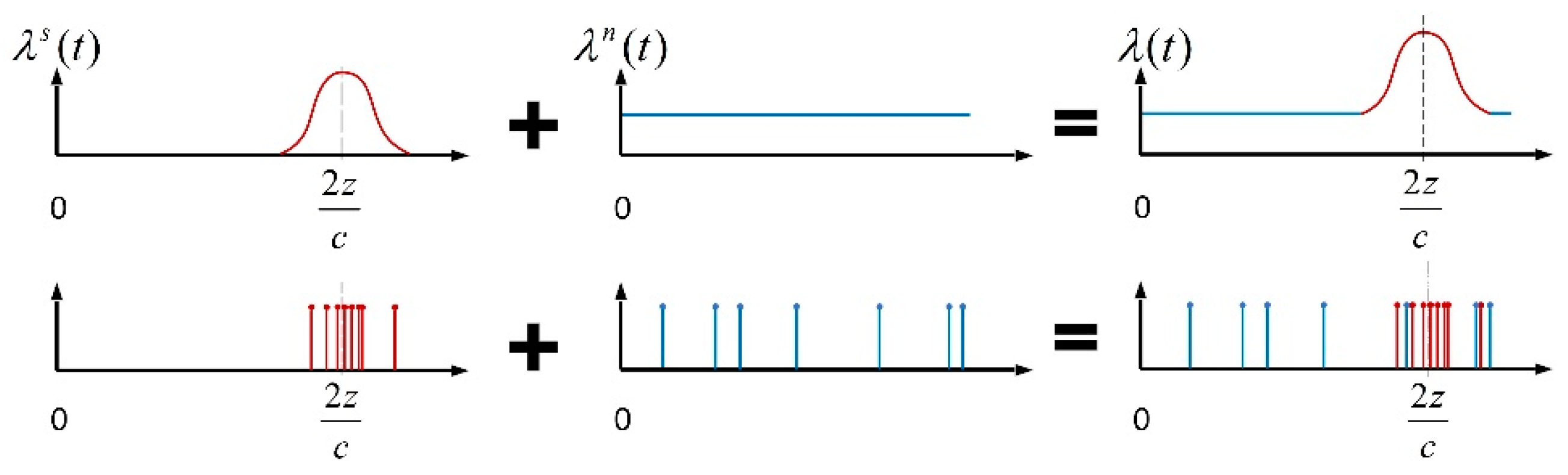
The overall photon-counting process is the Poisson point process [17], and it could be viewed as the sum of two independent Poisson processes, that is, signal inhomogeneous Poisson process and noise homogenous Poisson process. The rate of signal Poisson process is actually concentrated within pulse width, whereas the rate of noise Poisson process is flat. Considering the low light level environment, pile-up effect [18] or dead time effect could be ignored, and, accordingly, the time tags of signal counts and noise counts would obey Gaussian distribution (we suppose laser pulse waveform is Gaussian) and uniform distribution, respectively, as Figure 1 indicates.
According to Gaussian theory, the variance of signal time tags would be equal to where denotes root mean square (RMS) pulse width. Variance of noise time tags, from uniform distribution theory, would be 1/12 , where is the pulse repetition period. For , the most evident difference is that the variance in signal counts is rather tiny, while variance in noise counts is large, which means signal counts tend to cluster together and noise photons would occupy the whole temporal duration.
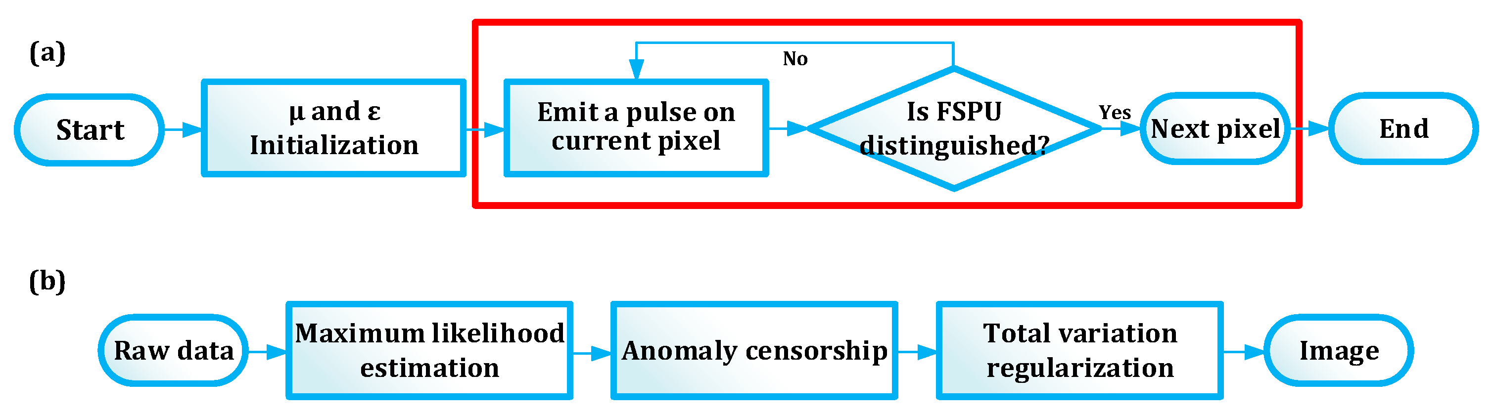
Exploiting this characteristic, we developed our FSPU method with two aspects; acquisition strategy and reconstruction strategy. The essence of acquisition strategy is straightforward and it can be briefly interpreted that we will not transfer to the next pixel until the first signal photon unit of current pixel has been distinguished. More specifically, we define two acquisition parameters, unit size and unit range . For each laser pulse, time tags of photon counts, if any, will be registered to system, and when the registered photon counts are found to be clustered, that is, photon counts within range in our method, we believe these counts are all due to signal photons and they are defined as FSPU, and then we transfer to next pixel. Figure 2 demonstrates our method.
Reconstruction strategy consists of three steps. The first step is to estimate range time through maximum likelihood estimation (MLE). Since we believe distinguished FSPU is caused by signal photons, the MLE of expectation of Gaussian is actually the average of FSPU as Equation (1) shows.
Subscript represents the -th row -th column pixel and means the time tag of -th count of FSPU. The second step is anomaly censorship. Although noise counts generally would not cluster, there is a chance that noise counts would meet the - criteria earlier than signal counts, and thusly they are falsely deemed as FSPU. In this step, for pixel , we will calculate the median value of its neighborhood and compare the pixel value with this median. If the pixel value is away from median, it is believed to be noisy. The underlying reason is that 95% signal counts would be within around expectation for Gaussian distribution. The noisy pixels would be replaced with their medians as Equation (2) demonstrates.
The third step is total variation (TV) regularization [19,20]. We add a TV penalty term to our estimated time image, as:
where is an size matrix whose -th row -th column element is and is the size of target image. TV is defined as:
Equation (3) is actually a minimum optimization problem where is a coefficient to make a trade-off between MLE data and correlations of adjacent pixels. In experiment, we used and its optimal value is the focus of our future research. After acquisition of reconstructed time image , range image is obtained by .
3. Simulations
To quantify our method performance, we first used the Middlebury dataset [21] to conduct simulations.
Figure 3a describes the distribution of signal counts numbers per pulse and Figure 3b is the truth range image . Signal counts were generated from an inhomogeneous Poisson process with as its rate where RMS width was set as 0.6 ns to maintain consistency with the laser used in our later experiment. Noise counts were generated from a homogeneous Poisson process with noise intensity as its rate. Image size and were set to be and 200 ns, respectively, in simulations. were chosen as 0.01 MHz, 0.1 MHz, 0.25 MHz, 0.5 MHz, 0.75 MHz and 1 MHz, consecutively, to generate several different noise levels. The mean SNR is evaluated as:
In the simulation, we chose and to be 5 and 1.2 ns, respectively, which meant our FSPU was defined as five counts within 1.2 ns temporal width. The reconstruction processes with are demonstrated in Figure 4.
We also reconstructed depth images using other methods such as peak, cross-correlation, unmixing [12] and FPI [13] to compare their performances with our FSPU method. Mean square error (MSE), defined as:
is utilized as a measure of reconstruction performance where is true depth of pixel . Efficiency is measured through the number of emitted pulses per pixel (ppp). Less pulses means less acquisition time and, thus, higher efficiency. Although numbers of pulses for each pixel vary for our FSPU and FPI, we can calculate the average number of pulses per pixel to evaluate efficiency, that is, total emitted pulses number divided by pixel size.
First, we ran our FSPU method, and the number of emitted pulses per pixel was obtained through above-mentioned calculation. To compare performances of these methods with a common baseline, we restricted the number of emitted pulses for each pixel of peak, cross-correlation and unmixing to be identical to our FSPU, which means we restricted the efficiency of these three methods to be the same as our method. The result is displayed in Figure 5.
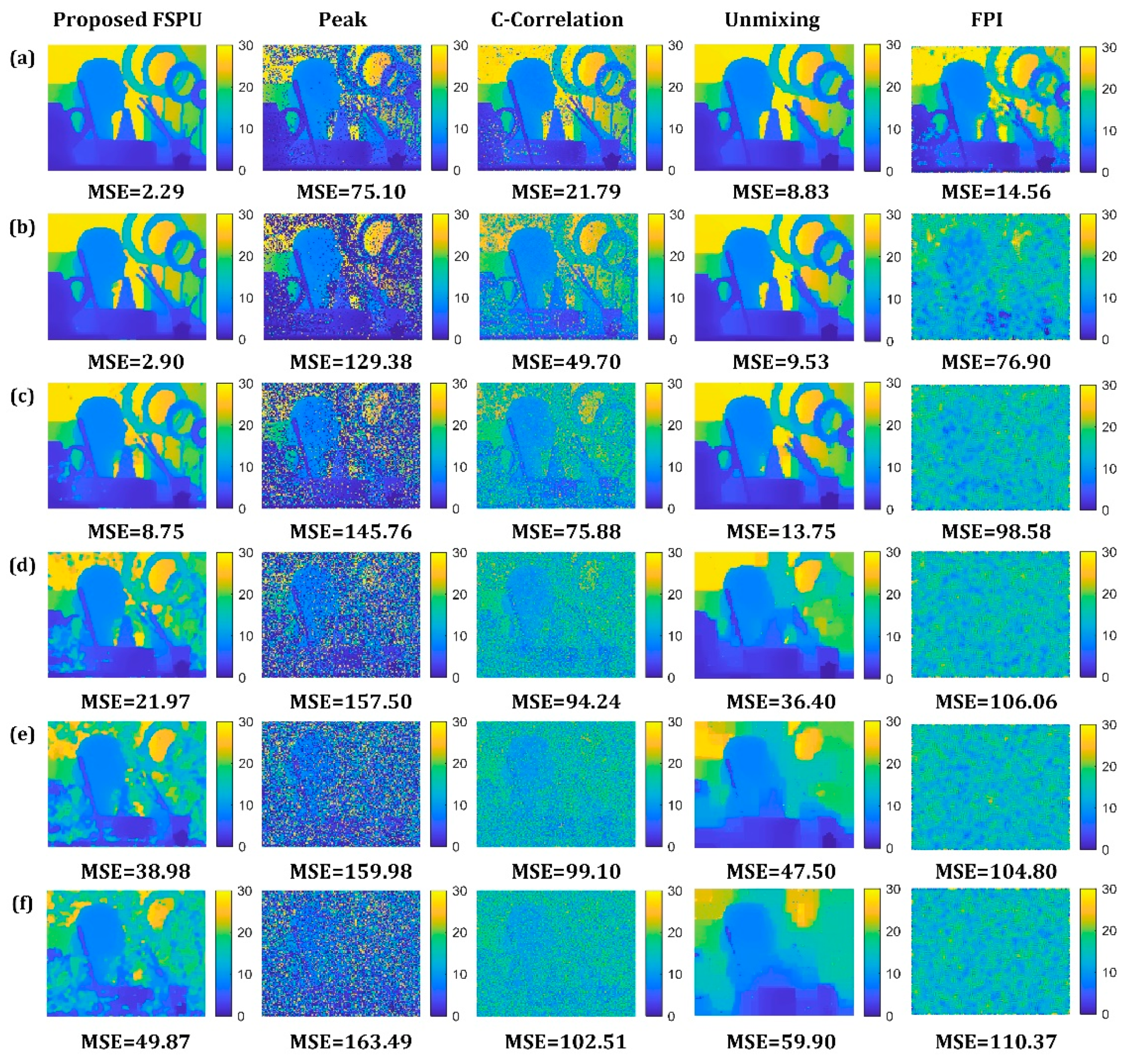
Although FPI is the most efficient method (FPI only needs 1 cpp to reconstruct images and therefore the number of emitted pulses is the lowest), it has poor performance, especially when SNR is low. For example, when SNR is lower than 0 dB, MSEs of FPI are large and the reconstructed images are almost nonsense because most of its first photon counts are noisy and they convey no range information. Emitted pulses number for the first four methods seems much larger than FPI; however, as signal is weak, the signal detections are essentially as few as several counts. The peak method is a traditional photon-counting imaging method which chooses the position of histogram peak as rang time. The cross-correlation method is to make a cross correlation between system instrument response function (IRF) and histogram, and then it finds the position of maximum value.
From Figure 5, we could see that MSEs of these three fixed acquisition time methods are larger than our method, which indicates the reconstruction performance of our method is much better. The result is intuitive because the pulses number is identical for each pixel for these three methods, which does not take pixel differences into consideration.
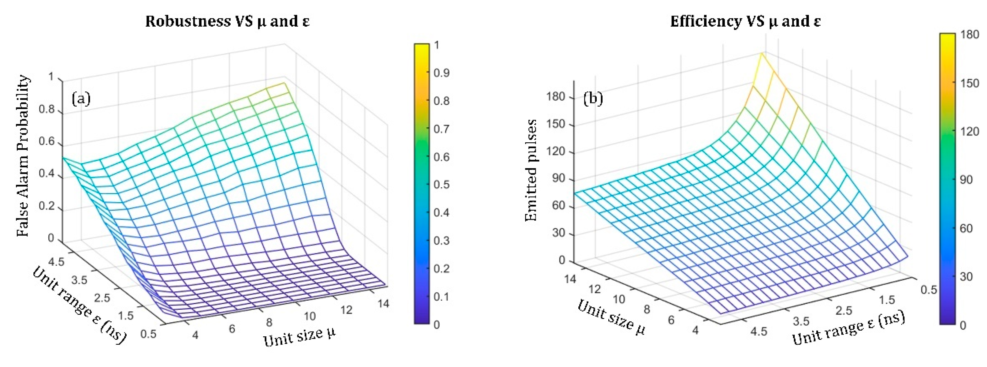
Actually, when SNR decreases, the image quality of our method worsens, as Figure 5 shows. For low SNR conditions, we can improve the quality by increasing or decreasing to further avoid false clusters, although this may result in lower efficiency. Monte Carlo simulations were conducted to demonstrate how and influence efficiency and robustness, as Figure 6 indicates.
Here we set noise intensity as 0.25 MHz, signal photon number as 0.01 per pulse and RMS laser width as 0.6 ns. If counts of a FSPU are all due to noise, it is deemed as a false alarm. From Figure 6, we could notice that larger and smaller would promote robustness, but reduce efficiency. In fact, the method allows us to make a trade-off between efficiency and noise robustness through and . The method is actually an extension of FPI. When , it would be simplified to be FPI, which only focuses on imaging efficiency. In addition, background noise calibration is not required in our method. We only need to know an approximate level of noise to provide information to choose and , instead of measuring accurate noise distribution of each pixel which is generally a time-consuming task. Experience shows and would be reliable choices for a variety of scenarios.
4. Experiments
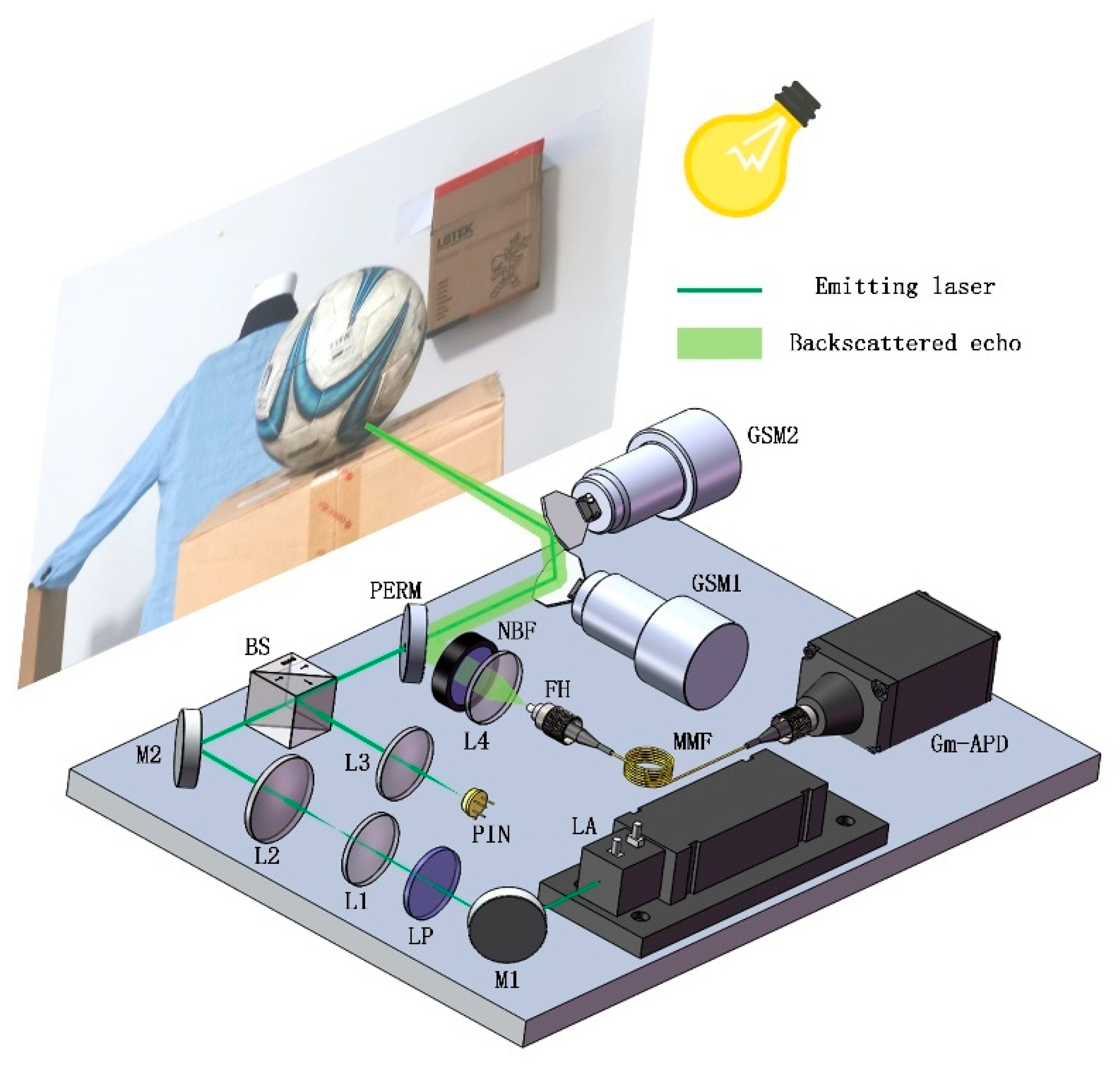
To explore the performance of the method in a real imaging environment, we carried out experiments in a laboratory. The photon-counting LIDAR system is designed as Figure 7 demonstrates.
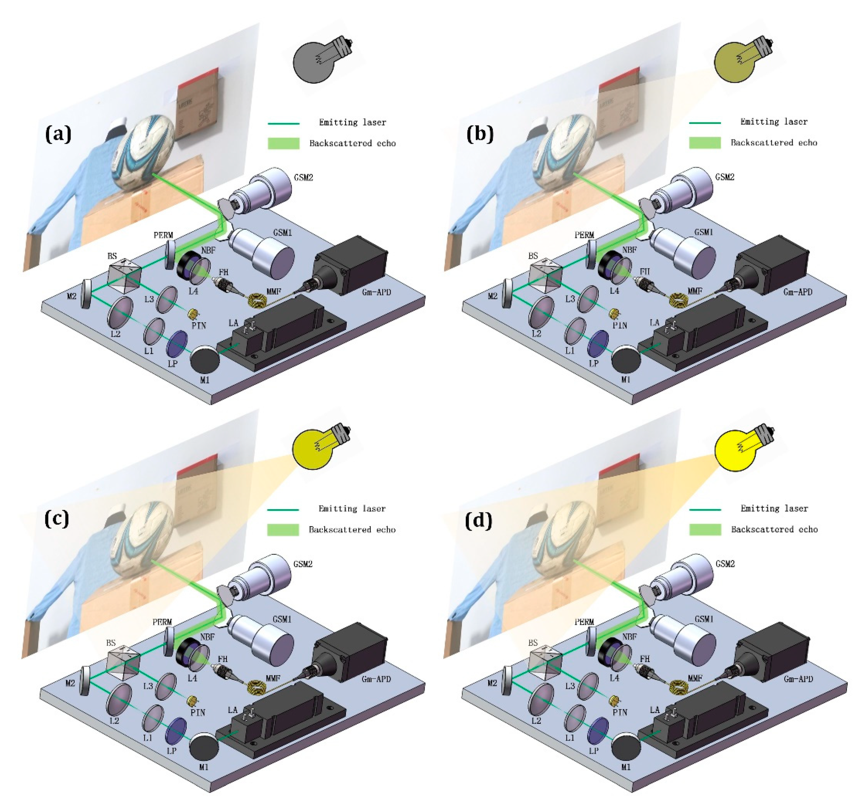
Laser (CryLaS FDSS532) emits pulses at the fixed repetition rate of 10 KHz. Mirror 1 deflects the laser beam at 90° into a linear polarizer. As the laser beam is linearly polarized from the laser, rotating the polarizer can adjust pulse energy afterwards. Two lenses, L1 and L2, are jointly used as beam expander to lower down laser divergence. A beam splitter deflects 1% beam into a PIN photodiode, the signal from which serves as start baseline. The remaining 99% beam continues its travel through a perforated mirror and then emits out to scenes of interest by two galvo scanning mirrors (Thorlabs GVS012). The back reflected echo photons enter the system in the same way and as the reflected beam is diffusely scattered, most of it would be deflected by the PERM into the receiving part. NBF moves away noise photons which are out of emitting wavelength. Eventually, the echo photons are coupled into a multimode fiber that connects to the Gm-APD (Micro Photon Devices PDM series $PD-050-CTC-FC whose photon detection efficiency is about 42% for 532 nm wavelength and dead time is 77 ns) at the other end. A gate of 200 ns was utilized to block system back-reflection light.
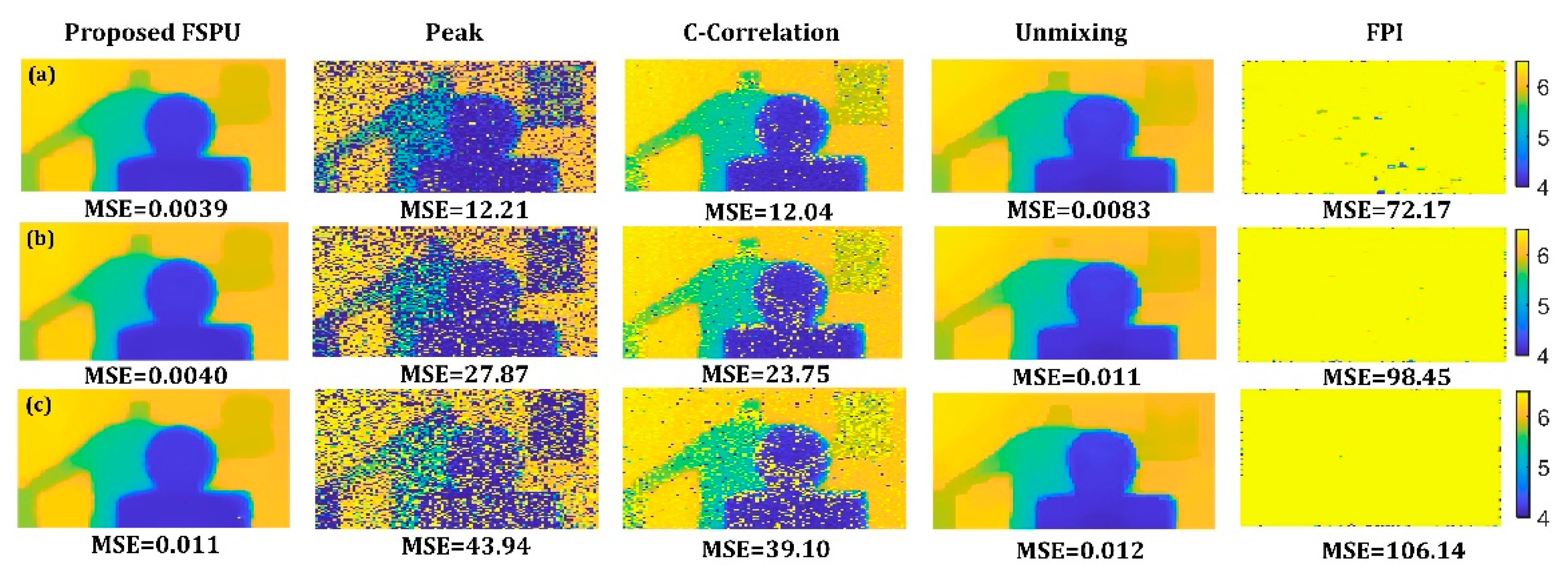
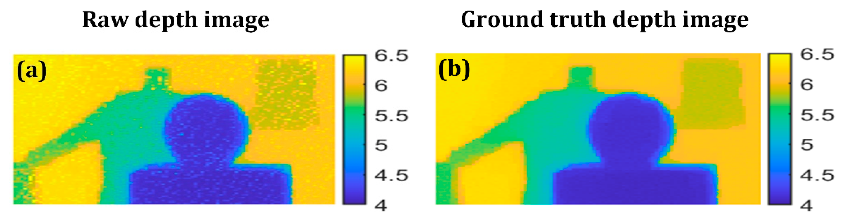
A football, a man-made mannequin, a box and the background wall were about 4.0 m, 5.5 m, 5.8 m and 6.1 m away from the front of our photon-counting LIDAR, respectively. The setup was placed in dark laboratory environment and an incandescent lamp with adjustable illumination was utilized as the source of noise. Details of the experiment are included in Appendix A. During the experiment, the echo level was extremely low. The signal counts level, on average, was about 0.0074 per pulse which meant that every 135 pulses would only generate 1 signal count. Three noise levels, the corresponding SNR of which were −5.14 dB, −8.35 dB and −10.85 dB, were achieved through the adjustment of the lamp. The result of the experiment is demonstrated in Figure 8.
Acquisition of the ground truth depth image and signal-noise evaluation processes are available in Appendix A. From the result, our method shows better MSEs compared to others. FPI, without any doubt, is the most efficient method, but it suffers much larger error to be almost noninformative. Results of the experiment have the same tendency as simulation. For the same total acquisition time (which means the same efficiency), our method could recover higher quality depth image, which, on the other hand, reveals that to obtain the same quality image, our method would require much less time. The experiment data and code are provided as we show in the Supplementary Material.
It is worth noting that MSEs of the unmixing method are also tiny, almost the same as our FSPU method. However, the unmixing method needs accurate noise levels to reconstruct clear images, while our method does not require such information. In this experiment, noise levels were evaluated beforehand and if noise levels are unknown, the unmixing method would have much worse reconstruction quality.
5. Discussion and Conclusions
In conclusion, we reported an efficient and noise robust photon-counting imaging method which is specifically suitable for low signal and high noise environments such as daylight imaging or underwater imaging. The method exploits the statistical difference that signal would cluster while noise would decentralize, in order to distinguish signal counts rapidly. The acquisition time of each pixel is a photon level-dependent variable and background noise calibration is not needed any more. The method is an extension of FPI and it outperforms the mainstreaming photon-counting methods in low SNR scenarios. By introducing two acquisition parameters and , the method allows users to make a trade-off between efficiency and robustness. For example, when SNR is low, larger and smaller would be helpful to avoid noise, although acquisition time might be longer. More importantly, the method does not need noise calibrations. Although it is not mentioned in the paper, the method has the ability to recover reflectivity images with the elapsed pulse number of each pixel. However, the elapsed pulse number is not only related to reflectivity, but also to noise level, and there is no such a mature theory or analytical solution to settle this problem, which is the priority of our future work.
Supplementary Materials
Supplementary materials are available online at https://www.mdpi.com/article/10.3390/photonics8060229/s1.
Author Contributions
Conceptualization, K.H. and B.L.; funding acquisition, Z.C.; methodology, K.H.; software, K.H.; supervision, B.L.; validation, H.W.; visualization, K.H.; writing—original draft, K.H.; writing—review and editing, Z.C. and L.F. All authors have read and agreed to the published version of the manuscript.
Funding
This research was funded by National Natural Science Foundation of China, grant number 61805249 and Youth Innovation Promotion Association of the Chinese Academy of Sciences, grant number 2019369.
Data Availability Statement
Experiment data and reconstruction code presented in this study are available in supplementary material.
Acknowledgments
Portions of this work were presented at the SPIE, the Seventh International Symposium on Novel Optoelectronic Detection Technology and Application in 2020, efficient and noise robust photon-counting imaging method.
Conflicts of Interest
The authors declare no conflict of interest.
Appendix A
To keep the primary article concise, details of the experiment, data format and reconstruction processing are provided in this appendix.
Appendix A.1. Details of Experiment
Stage 1 (none): First, we turned on the laser with the lamp off, as Figure A1a shows, and rotated the polarizer to set the intensity of signal photons to an extremely low level to simulate weak echo. Then, we started our imaging of 100 × 100 pixels with 2 s acquisition time for each pixel (namely 20 K pulses) and data was collected through SIMINICS (FT1020) time correlated single photon counter (TCSPC) as photon_counts_data_none in the Supplementary Material. Since the lamp was off, photon counts were almost assumed to be due to signal, and using this dataset we reconstructed depth image as ground truth image, which is represented in the next section. Thereafter, we fixed the polarizer to keep the echo level unchanged. Then, we aimed to scan the scene with different noise levels.
Stage 2 (low): We adjusted the illumination of the lamp to low intensity, as Figure A1b shows. We raster scanned the scenes with the same 2 s acquisition time for each pixel and the same scanning resolution, and registered every photon count. A photon count dataset for low noise intensity was therefore acquired, which is named photon_counts_data_low in the Supplementary Material.
Stage 3 (middle): Similarly, we adjusted the illumination of the lamp to middle intensity, as Figure A1c shows. We also raster scanned the scenes with the same 2 s acquisition time for each pixel and the same scanning resolution, and registered every photon count. A photon count dataset for middle noise intensity was therefore acquired, which is named photon_counts_data_mid in the Supplementary Material.
Stage 4 (high): In the same way, we adjusted the illumination of the lamp to high intensity, as Figure A1d shows. We also raster scanned the scenes with the same 2 s acquisition time for each pixel and the same scanning resolution, and registered every photon count. A photon count dataset for high noise intensity was therefore acquired, which is named photon_counts_data_high in the Supplementary Material.
Figure A1.
Demonstration of experiment details. (a) Dark experiment. (b) Low noise intensity experiment. (c) Middle noise intensity experiment. (d) High noise intensity experiment.
Figure A1.
Demonstration of experiment details. (a) Dark experiment. (b) Low noise intensity experiment. (c) Middle noise intensity experiment. (d) High noise intensity experiment.

Appendix A.2. Evaluation of Signal and Noise Level
Before our reconstruction, we needed to quantify the levels of signal and noise. The signal level can be evaluated by finding the number of photon_counts_data_none minus the number of detector dark counts. The detector’s dark count is 100 Hz according to its specification sheet which is 4 K for the whole dataset with consideration of 200 ns gate time, 20 K accumulation pulses and pixel size. Consequently, the overall signal counts number is estimated as 1.49 M. On average, for each pixel, the signal count level is 0.00744 per pulse, which means that more than 134 pulses would generate only one signal count.
Since we fixed a linear polarizer to keep the echo level unchanged, the noise count number of photon_counts_data_low can be simply evaluated through the counts of photon_counts_data_low minus previously obtained signal counts. Similar evaluations have also been applied to photon_counts_data_mid and photon_counts_data_high. The result indicated that the noise levels (with the consideration of photon detection efficiency) were 0.29 M, 0.61 M and 1.08 M, respectively, and their corresponding SNRs were −5.14 dB, −8.35 dB and −10.85 dB.
Appendix A.3. Ground Truth Depth Image
The dataset of photon_counts_data_none was utilized to recover the ground truth image because it is assumed to include only a few of dark noise counts. First, we filtered out dark noise counts using a straightforward median-like pixel-wise method. For each pixel, we calculated the median of its counts and compared every count with this median. If count time is away from the median ( is RMS pulse width of IRF), this count is believed to be a dark noise count, and therefore would be abandoned. After dark noise filter, we recovered the ground truth depth image, simply using the mean of unfiltered counts. Figure A2 demonstrates depth images reconstructed from photon_counts_data_none with and without dark counts filter processing.
Figure A2.
Depth image from dark experiment dataset. (a) Reconstruction using the mean of counts without dark noise counts filtering. (b) Reconstruction using the mean of counts with dark noise counts filtering.
Figure A2.
Depth image from dark experiment dataset. (a) Reconstruction using the mean of counts without dark noise counts filtering. (b) Reconstruction using the mean of counts with dark noise counts filtering.

Appendix A.4. Reconstruction Process
In this experiment, we used the same data set for our FSPU method and other methods to evaluate their performances. For our reconstruction process, we added photon counts from the dataset one-by-one, and when FSPU was discovered, we transferred to next pixel data. FPI operated in similar way to only use the first photon count of each pixel. After our FSPU method, average emitted pulses per pixel could be obtained and for each pixel, we only included photon counts generated by first pulses to reconstruct depth images with peak, cross-correlation and unmixing methods to maintain the same efficiency (same baseline) for performance comparison.
Appendix A.5. Dataset Format
There are four experiment datasets and one SNR dataset provided in our Supplementary Material. They are .m files which are readable with Matlab. Each experiment dataset has two cell arrays which represent time and synchronization information under different noise levels for each pixel. SNR contains information of evaluated signal level and noise levels.
References
- Massa, J.S.; Wallace, A.M.; Buller, G.; Fancey, S.J.; Walker, A.C. Laser depth measurement based on time-correlated single-photon counting. Opt. Lett. 1997, 22, 543–545. [Google Scholar] [CrossRef] [PubMed] [Green Version]
- McCarthy, A.; Collins, R.J.; Krichel, N.J.; Fernández, V.; Wallace, A.M.; Buller, G.S. Long-range time-of-flight scanning sensor based on high-speed time-correlated single-photon counting. Appl. Opt. 2009, 48, 6241–6251. [Google Scholar]
- McCarthy, A.; Ren, X.; Frera, A.D.; Gemmell, N.R.; Krichel, N.J.; Scarcella, C.; Ruggeri, A.; Tosi, A.; Buller, G.S. Kilome-ter-range depth imaging at 1550 nm wavelength using an InGaAs/InP singlephoton avalanche diode detector. Opt. Express 2013, 21, 22098–22113. [Google Scholar] [CrossRef] [PubMed] [Green Version]
- Li, L.; Huang, X.; Cao, Y.; Wang, B.; Li, Y.; Jin, W.; Yu, C.; Zhang, J.; Zhang, Q.; Peng, C.; et al. Single-photon compu-tational 3D imaging at 45 km. Photon. Res. 2020, 8, 1532–1540. [Google Scholar] [CrossRef]
- Pawlikowska, A.M.; Halimi, A.; Lamb, R.A.; Buller, G.S. Single-photon three-dimensional imaging at up to 10 kilometers range. Opt. Express 2017, 25, 11919–11931. [Google Scholar] [CrossRef] [PubMed]
- Neumann, T.A.; Martino, A.J.; Markus, T.; Bae, S.; Bock, M.R.; Brenner, A.C.; Brunt, K.M.; Cavanaugh, J.; Fernandes, S.T.; Hancock, D.W.; et al. The Ice, Cloud, and Land Elevation Satellite—2 mission: A global geolocated photon product derived from the Advanced Topographic Laser Altimeter System. Remote Sens. Environ. 2019, 233, 111325. [Google Scholar] [CrossRef] [PubMed]
- Yan, K.; Lifei, L.; Xuejiec, D.; Tongyia, Z.; Dongjiana, L.; Weia, Z. Photon-limited depth and reflectivity imaging with sparsity regularization. Opt. Commun. 2017, 392, 25–30. [Google Scholar]
- Halimi, A.; Altmann, Y.; McCarthy, A.; Ren, X.; Tobin, R.; Buller, G.S.; McLaughlin, S. Restoration of intensity and depth images constructed using sparse single-photon data. In Proceedings of the 2016 24th European Signal Processing Conference (EUSIPCO); Institute of Electrical and Electronics Engineers (IEEE), Budapest, Hungary, 29 August–2 September 2016; pp. 86–90. [Google Scholar]
- Shin, D.; Kirmani, A.; Goyal, V.K.; Shapiro, J.H. Photon-Efficient Computational 3-D and Reflectivity Imaging with Single-Photon Detectors. IEEE Trans. Comput. Imaging 2015, 1, 112–125. [Google Scholar] [CrossRef] [Green Version]
- Kirmani, A.; Colaço, A.; Wong, N.C.; Goyal, V.K. Exploiting sparsity in time-of-flight range ac-quisition using a single time-resolved sensor. Opt. Express 2011, 19, 21485–21507. [Google Scholar] [CrossRef] [PubMed]
- Altmann, Y.; Ren, X.; McCarthy, A.; Buller, G.S.; McLaughlin, S. Robust Bayesian target detection algorithm for depth imaging from sparse single-photon data. IEEE Trans. Comput. Imaging 2016, 2, 1. [Google Scholar] [CrossRef] [Green Version]
- Rapp, J.; Goyal, V. A Few Photons among Many: Unmixing Signal and Noise for Photon-Efficient Active Imaging. IEEE Trans. Comput. Imaging 2017, 3, 445–459. [Google Scholar] [CrossRef]
- Chen, W.; Li, S.; Tian, X. Robust single-photon counting imaging with spatially correlated and total variation constraints. Opt. Express 2020, 28, 2625–2639. [Google Scholar] [CrossRef] [PubMed]
- Kirmani, A.; Venkatraman, D.; Shin, D.; Colaço, A.; Wong, F.N.C.; Shapiro, J.H.; Goyal, V.K. First-Photon Imaging. Science 2014, 343, 58–61. [Google Scholar] [CrossRef] [PubMed]
- Kirmani, A.; Venkatraman, D.; Shin, D.; Colaco, A.; Wong, F.N.C.; Shapiro, J.H.; Goyal, V.K. Supporting Materials for First-Photon Imaging. 2014. Available online: http://www.sciencemag.org/content/343/6166/58/suppl/DC1 (accessed on 19 June 2021).
- Kirmani, A.; Shin, D.; Venkatraman, D.; Wong, F.N.C.; Goyal, V.K. First-Photon Imaging: Scene Depth and Reflectance Acquisition from One Detected Photon per Pixel. In Proceedings of the 2013 IEEE International Conference on Computer Vision (ICCV ’13), Sydney, NSW, Australia, 1–8 December 2013; pp. 449–456. [Google Scholar]
- Fouche, D.G. Detection and false-alarm probabilities for laser radars that use Geiger-mode detectors. Appl. Opt. 2003, 42, 5388–5398. [Google Scholar] [CrossRef] [PubMed]
- O’Connor, D.V.; Phillips, D. Time-Correlated Single Photon Counting; Elsevier BV: London, UK, 1984. [Google Scholar]
- Beck, A.; Teboulle., M. Fast Gradient-Based Algorithms for Constrained Total Variation Image Denoising and Deblurring Problems. IEEE Trans. Image Process. 2009, 11, 2419–2434. [Google Scholar] [CrossRef] [PubMed] [Green Version]
- Rudin, L.I.; Osher, S.; Fatemi, E. Nonlinear total variation based noise removal algorithms. Phys. D Nonlinear Phenom. 1992, 60, 259–268. [Google Scholar] [CrossRef]
- Scharstein, D.; Pal, C. Learning Conditional Random Fields for Stereo. In Proceedings of the 2007 IEEE Conference on Computer Vision and Pattern Recognition; Institute of Electrical and Electronics Engineers (IEEE), Minneapolis, MN, USA, 17–22 June 2007; pp. 1–8. [Google Scholar]
Figure 1.
Signal and noise Poisson model, , and are signal rate, noise rate and total rate respectively, is depth and is velocity of light.
Figure 1.
Signal and noise Poisson model, , and are signal rate, noise rate and total rate respectively, is depth and is velocity of light.

Figure 2.
Block diagrams of our FSPU method. (a) Block flowchart of acquisition strategy. Processes inside red box would be repeatedly executed until data for all pixels has been obtained. (b) Block flowchart of reconstruction strategy.
Figure 2.
Block diagrams of our FSPU method. (a) Block flowchart of acquisition strategy. Processes inside red box would be repeatedly executed until data for all pixels has been obtained. (b) Block flowchart of reconstruction strategy.

Figure 3.
Middlebury dataset image for simulation. (a) Image of averaged signal photon per pulse; (b) depth image.
Figure 3.
Middlebury dataset image for simulation. (a) Image of averaged signal photon per pulse; (b) depth image.

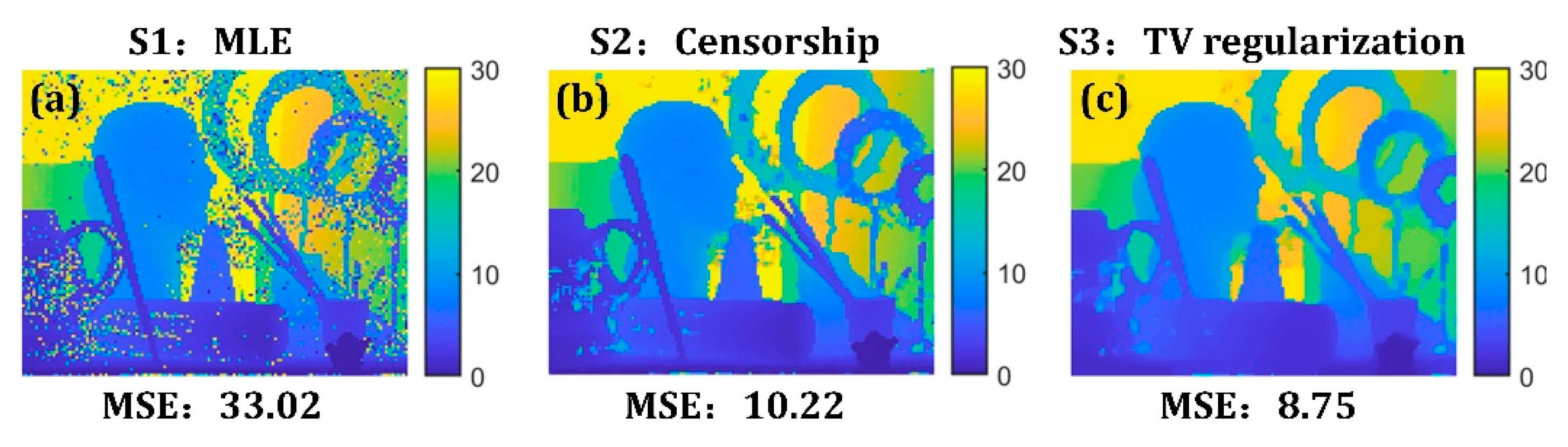
Figure 4.
FSPU reconstruction steps; on average, 2700 pulses per pixel (ppp) were emitted with 67.8 counts per pixel (cpp), 89% of which, however, were noise counts. (a) Step1: Maximum likelihood estimation, (b) Step2: anomaly censorship, (c) Step3: TV regularization.
Figure 4.
FSPU reconstruction steps; on average, 2700 pulses per pixel (ppp) were emitted with 67.8 counts per pixel (cpp), 89% of which, however, were noise counts. (a) Step1: Maximum likelihood estimation, (b) Step2: anomaly censorship, (c) Step3: TV regularization.

Figure 5.
Performance comparison between methods on different noise levels. (a) 0.01 MHz noise (SNR = 4.5 dB), 3183 ppp for the first four methods, 335 ppp for FPI; (b) 0.1 MHz noise (SNR = −5.5 dB), 3313 ppp, 81 ppp; (c) 0.25 MHz noise (SNR = −9.5 dB), 2514 ppp, 37 ppp; (d) 0.5 MHz noise (SNR = −12.5 dB), 1755 ppp, 20 ppp; (e) 0.75 MHz noise (SNR = −14.3 dB), 1358 ppp, 14 ppp; (f) 1 MHz noise (SNR = −15.5 dB), 1088 ppp 10 ppp.

Figure 6.
The relationship between - and efficiency-robustness. (a) Influence of - on robustness; (b) influence of - on noise efficiency.
Figure 6.
The relationship between - and efficiency-robustness. (a) Influence of - on robustness; (b) influence of - on noise efficiency.

Figure 7.
Illustration of our photon-counting experiment. LA, laser; M, mirror; LP, linear polarizer; L, lens; BS, beam splitter; PIN, pin photodiode; PERM, perforated mirror; NBF, narrow bandpass filter; FH, fiber head; MMF, multimode fiber; Gm-APD, Geiger mode avalanche photodiode; GSM, galvo scanning mirror. Scene of interest includes a mannequin, a football and a box.

Figure 8.
Experimental result. (a) Low noise level, 953 ppp for first four methods, 38 ppp for FPI; (b) mid noise level, 916 ppp, 21 ppp; (c) high noise level, 845 ppp, 13 ppp.
Figure 8.
Experimental result. (a) Low noise level, 953 ppp for first four methods, 38 ppp for FPI; (b) mid noise level, 916 ppp, 21 ppp; (c) high noise level, 845 ppp, 13 ppp.

Publisher’s Note: MDPI stays neutral with regard to jurisdictional claims in published maps and institutional affiliations. |
© 2021 by the authors. Licensee MDPI, Basel, Switzerland. This article is an open access article distributed under the terms and conditions of the Creative Commons Attribution (CC BY) license (https://creativecommons.org/licenses/by/4.0/).
Share and Cite
MDPI and ACS Style
Hua, K.; Liu, B.; Chen, Z.; Fang, L.; Wang, H. Efficient and Noise Robust Photon-Counting Imaging with First Signal Photon Unit Method. Photonics 2021, 8, 229. https://doi.org/10.3390/photonics8060229
AMA Style
Hua K, Liu B, Chen Z, Fang L, Wang H. Efficient and Noise Robust Photon-Counting Imaging with First Signal Photon Unit Method. Photonics. 2021; 8(6):229. https://doi.org/10.3390/photonics8060229
Chicago/Turabian StyleHua, Kangjian, Bo Liu, Zhen Chen, Liang Fang, and Huachuang Wang. 2021. "Efficient and Noise Robust Photon-Counting Imaging with First Signal Photon Unit Method" Photonics 8, no. 6: 229. https://doi.org/10.3390/photonics8060229
Note that from the first issue of 2016, this journal uses article numbers instead of page numbers. See further details here.