
Applications of Machine Learning (ML) and Mathematical Modeling (MM) in Healthcare with Special Focus on Cancer Prognosis and Anticancer Therapy: Current Status and Challenges

 , , ,
, , ,  and
and 
Abstract
:1. Introduction
1.1. General Concepts of Machine Learning (ML) and Mathematical Modeling (MM)
1.1.1. ML
1.1.2. MM
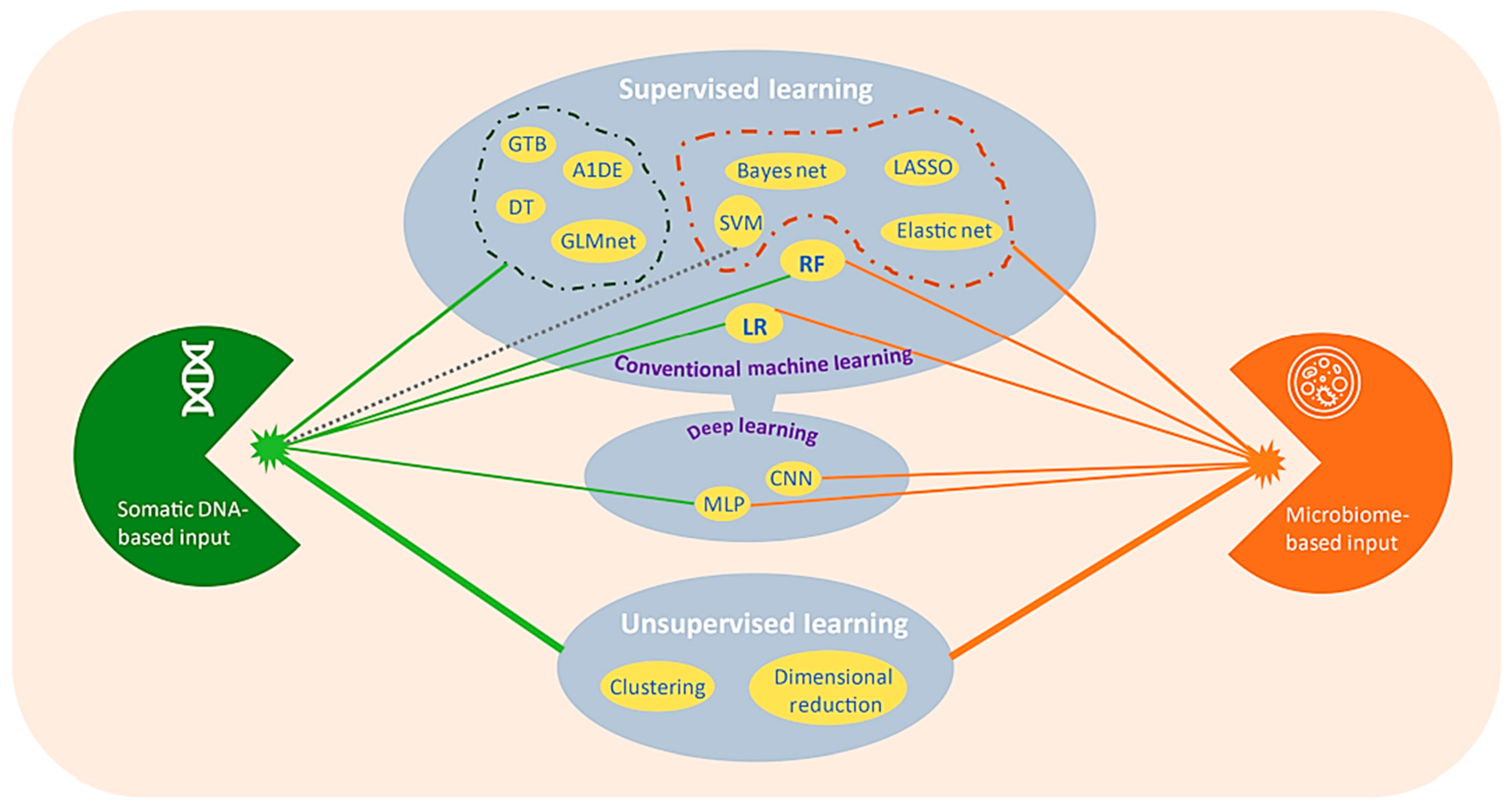
2. Paradigms of ML
2.1. Supervised ML
2.2. Unsupervised ML
2.3. Reinforced Learning
3. ML and MM Approaches in Healthcare
3.1. Discovery of New Drug Molecule
3.2. Prediction and Management of Global Pandemic
3.3. Epigenomics

| Area of Purpose | ML Tools | Prediction Details | Challenges | Reference(s) |
|---|---|---|---|---|
| Protein sequencing | ResNets, 2D convolutional neural networks (CNNs) | Structure | Data accessibility is tough, and leakage of these data make the evaluation tougher | [219] |
| Multilayer perceptrons with windowing | Function | [220] | ||
| Transformers | Protein–protein interaction | [221] | ||
| Gene sequencing | 1D CNNs | Accessibility of genome | Genome contains repetition of codes | [222] |
| Recurrent neural networks (RNNs) | Arrangement of 3D genome | Missing data of interest | [223] | |
| Transformers | Interactions between enhancer and promoter | Lengthy sequences | [224] | |
| Genetic expression | Clustering | Intergenic interactions or co-expression | Link between function and co-expression is not clear | [225] |
| CNNs | Multidimensional | |||
| Autoencoders | Organizing transcription machinery | Loud noise | [226] | |
| Interactions between proteins | GCNs | Side effects of poly-pharmacology | Networks for interactions can be incomplete | [227] |
| Graph embedding | Protein function | Protein’s interaction depends on cellular location | [228] | |
| Number of possible combinations is higher |
3.4. Protein Engineering
4. ML Algorithms in Specific Types of Cancer
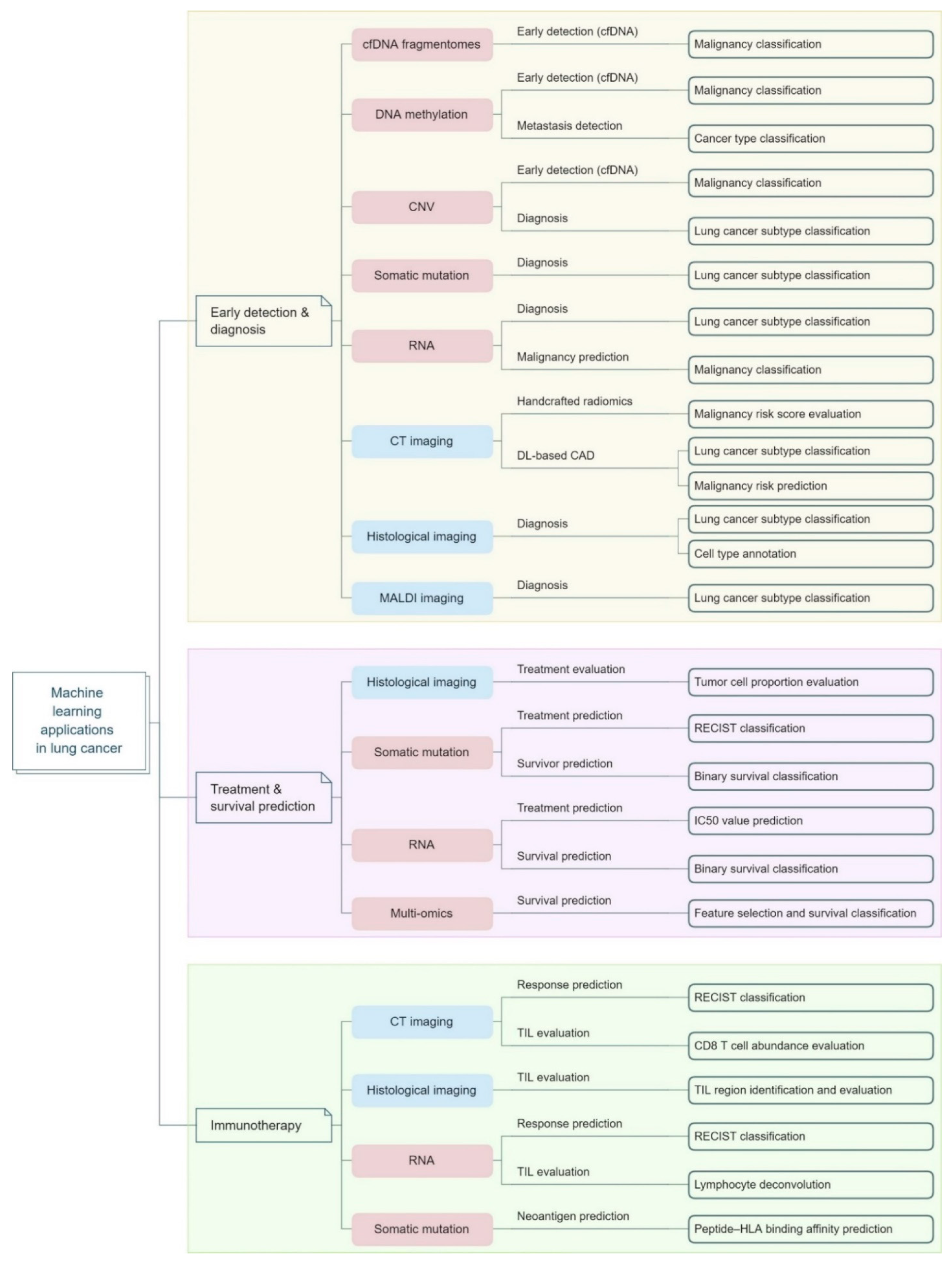
4.1. Lung Cancer
4.2. Colon Cancer
4.3. Pancreatic Cancer
4.4. Glioma
4.5. Skin Cancer
4.6. Oral Cancer
5. MM Techniques in Specific Types of Cancer
5.1. Tumor Growth
5.2. Treatment
5.3. Interconnection between ML and MM
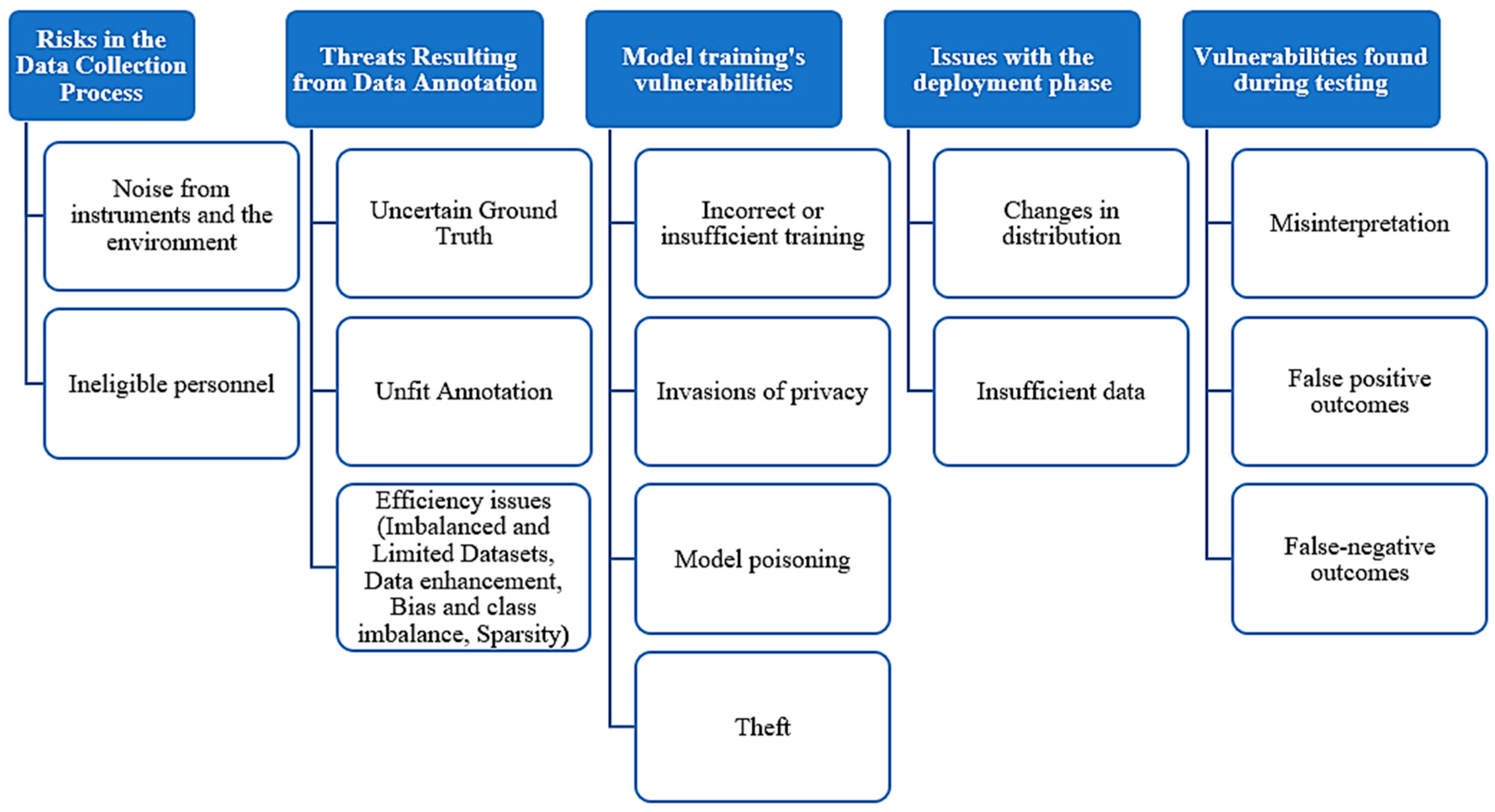
6. Challenges of ML and MM Approaches in Cancer Prognosis and Therapy
6.1. Data Quantity
6.2. Ethical Consideration
6.3. Data Privacy
7. Further Discussion and Future Directions
8. Conclusions
Author Contributions
Funding
Data Availability Statement
Conflicts of Interest
References
- Xue, C.; Chu, Q.; Zheng, Q.; Jiang, S.; Bao, Z.; Su, Y.; Lu, J.; Li, L. Role of Main RNA Modifications in Cancer: N6-Methyladenosine, 5-Methylcytosine, and Pseudouridine. Signal Transduct. Target. Ther. 2022, 7, 142. [Google Scholar] [CrossRef]
- Wang, Y.; Han, Y.; Jin, Y.; He, Q.; Wang, Z. The Advances in Epigenetics for Cancer Radiotherapy. Int. J. Mol. Sci. 2022, 23, 5654. [Google Scholar] [CrossRef]
- Jiang, W.; Liang, M.; Lei, Q.; Li, G.; Wu, S. The Current Status of Photodynamic Therapy in Cancer Treatment. Cancers 2023, 15, 585. [Google Scholar] [CrossRef]
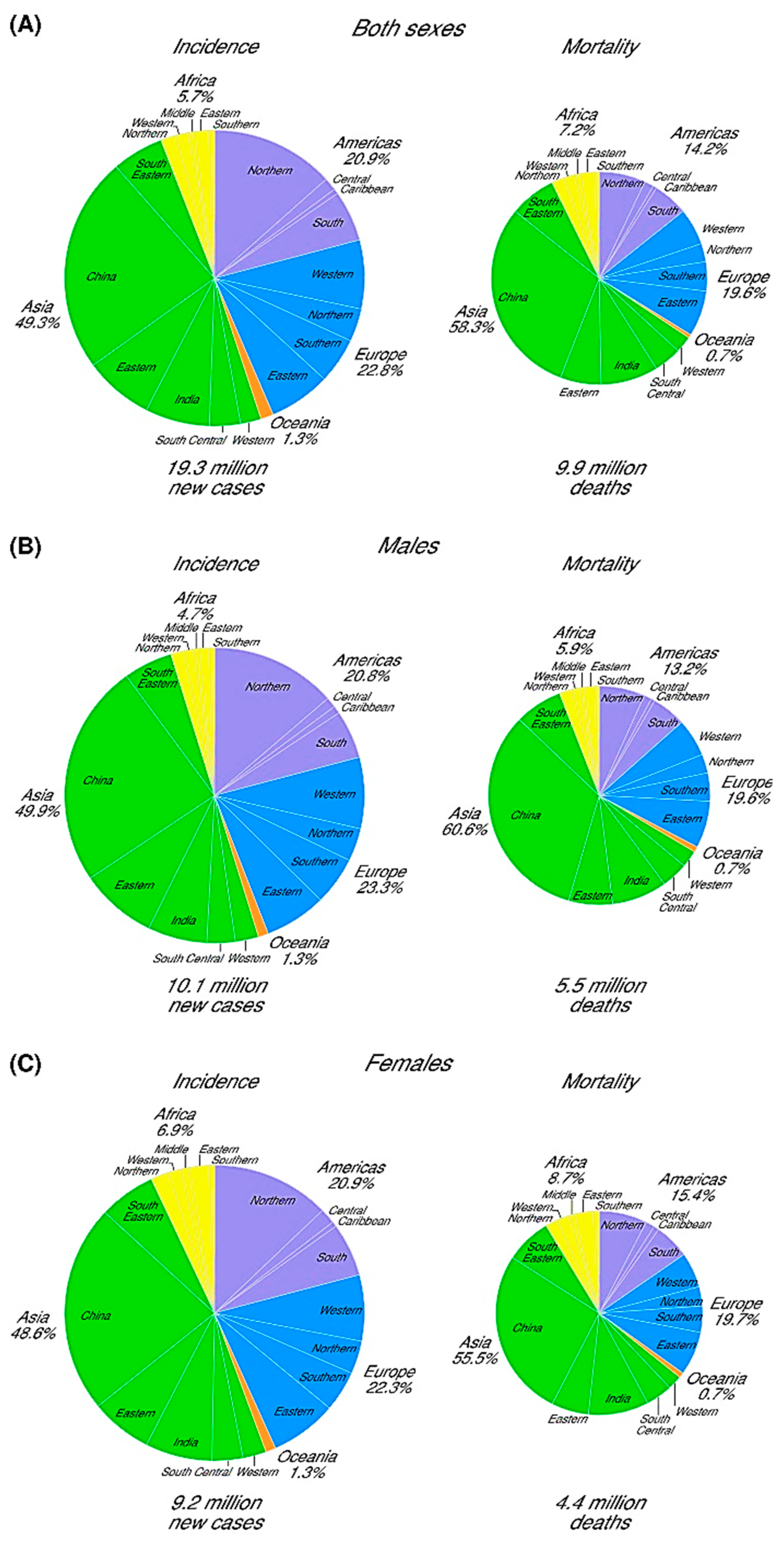
- Bray, F.; Ferlay, J.; Soerjomataram, I.; Siegel, R.L.; Torre, L.A.; Jemal, A. Global Cancer Statistics 2018: GLOBOCAN Estimates of Incidence and Mortality Worldwide for 36 Cancers in 185 Countries. CA. Cancer J. Clin. 2018, 68, 394–424. [Google Scholar] [CrossRef]
- Sung, H.; Ferlay, J.; Siegel, R.L.; Laversanne, M.; Soerjomataram, I.; Jemal, A.; Bray, F. Global Cancer Statistics 2020: GLOBOCAN Estimates of Incidence and Mortality Worldwide for 36 Cancers in 185 Countries. CA. Cancer J. Clin. 2021, 71, 209–249. [Google Scholar] [CrossRef] [PubMed]
- Li, J.; Wang, S.; Fontana, F.; Tapeinos, C.; Shahbazi, M.A.; Han, H.; Santos, H.A. Nanoparticles-Based Phototherapy Systems for Cancer Treatment: Current Status and Clinical Potential. Bioact. Mater. 2023, 23, 471–507. [Google Scholar] [CrossRef] [PubMed]
- Baskar, R.; Lee, K.A.; Yeo, R.; Yeoh, K.W. Cancer and Radiation Therapy: Current Advances and Future Directions. Int. J. Med. Sci. 2012, 9, 193. [Google Scholar] [CrossRef] [PubMed]
- Liu, Y.; Yang, H.; Xiong, J.; Zhao, J.; Guo, M.; Chen, J.; Zhao, X.; Chen, C.; He, Z.; Zhou, Y.; et al. Icariin as an Emerging Candidate Drug for Anticancer Treatment: Current Status and Perspective. Biomed. Pharmacother. 2023, 157, 113991. [Google Scholar] [CrossRef] [PubMed]
- Chen, J.; Cong, X. Surface-Engineered Nanoparticles in Cancer Immune Response and Immunotherapy: Current Status and Future Prospects. Biomed. Pharmacother. 2023, 157, 113998. [Google Scholar] [CrossRef] [PubMed]
- Mohapatra, A.; Sathiyamoorthy, P.; Park, I.K. Metallic Nanoparticle-Mediated Immune Cell Regulation and Advanced Cancer Immunotherapy. Pharmaceutics 2021, 13, 1867. [Google Scholar] [CrossRef] [PubMed]
- Tie, Y.; Tang, F.; Wei, Y.Q.; Wei, X.W. Immunosuppressive Cells in Cancer: Mechanisms and Potential Therapeutic Targets. J. Hematol. Oncol. 2022, 15, 61. [Google Scholar] [CrossRef]
- Helissey, C.; Vicier, C.; Champiat, S. The Development of Immunotherapy in Older Adults: New Treatments, New Toxicities? J. Geriatr. Oncol. 2016, 7, 325–333. [Google Scholar] [CrossRef]
- Doi, K. Computer-Aided Diagnosis in Medical Imaging: Historical Review, Current Status and Future Potential. Comput. Med. Imaging Graph. 2007, 31, 198–211. [Google Scholar] [CrossRef]
- Wong, D.; Yip, S. Machine Learning Classifies Cancer. Nature 2018, 555, 446–447. [Google Scholar] [CrossRef]
- Kourou, K.; Exarchos, T.P.; Exarchos, K.P.; Karamouzis, M.V.; Fotiadis, D.I. Machine Learning Applications in Cancer Prognosis and Prediction. Comput. Struct. Biotechnol. J. 2015, 13, 8–17. [Google Scholar] [CrossRef]
- Cruz, J.A.; Wishart, D.S. Applications of Machine Learning in Cancer Prediction and Prognosis. Cancer Inform. 2006, 2, 59–78. [Google Scholar] [CrossRef]
- Munir, K.; Elahi, H.; Ayub, A.; Frezza, F.; Rizzi, A. Cancer Diagnosis Using Deep Learning: A Bibliographic Review. Cancers 2019, 11, 1235. [Google Scholar] [CrossRef] [PubMed]
- Rosenblatt, F. The Perceptron: A Probabilistic Model for Information Storage and Organization in the Brain. Psychol. Rev. 1958, 65, 386–408. [Google Scholar] [CrossRef] [PubMed]
- Jordan, M.I.; Mitchell, T.M. Machine Learning: Trends, Perspectives, and Prospects. Science 2015, 349, 255–260. [Google Scholar] [CrossRef] [PubMed]
- Hethcote, H.W. The Mathematics of Infectious Diseases. Soc. Ind. Appl. Math. Rev. 2000, 42, 599–653. [Google Scholar] [CrossRef]
- Chambers, R.B. The Role of Mathematical Modeling in Medical Research: “Research Without Patients?”. Ochsner J. 2000, 2, 218. [Google Scholar]
- Liu, Y.; Wu, R.; Yang, A. Research on Medical Problems Based on Mathematical Models. Mathematics 2023, 11, 2842. [Google Scholar] [CrossRef]
- Tarca, A.L.; Carey, V.J.; Chen, X.W.; Romero, R.; Drǎghici, S. Machine Learning and Its Applications to Biology. PLoS Comput. Biol. 2007, 3, e116. [Google Scholar] [CrossRef]
- Jiang, F.; Jiang, Y.; Zhi, H.; Dong, Y.; Li, H.; Ma, S.; Wang, Y.; Dong, Q.; Shen, H.; Wang, Y. Artificial Intelligence in Healthcare: Past, Present and Future. Stroke Vasc. Neurol. 2017, 2, 230–243. [Google Scholar] [CrossRef] [PubMed]
- Dilsizian, S.E.; Siegel, E.L. Artificial Intelligence in Medicine and Cardiac Imaging: Harnessing Big Data and Advanced Computing to Provide Personalized Medical Diagnosis and Treatment. Curr. Cardiol. Rep. 2014, 16, 441. [Google Scholar] [CrossRef] [PubMed]
- Murdoch, T.B.; Detsky, A.S. The Inevitable Application of Big Data to Health Care. JAMA 2013, 309, 1351–1352. [Google Scholar] [CrossRef] [PubMed]
- Kononenko, I. Machine Learning for Medical Diagnosis: History, State of the Art and Perspective. Artif. Intell. Med. 2001, 23, 89–109. [Google Scholar] [CrossRef] [PubMed]
- Iqbal, M.J.; Javed, Z.; Sadia, H.; Qureshi, I.A.; Irshad, A.; Ahmed, R.; Malik, K.; Raza, S.; Abbas, A.; Pezzani, R.; et al. Clinical Applications of Artificial Intelligence and Machine Learning in Cancer Diagnosis: Looking into the Future. Cancer Cell Int. 2021, 21, 270. [Google Scholar] [CrossRef] [PubMed]
- Hanahan, D.; Weinberg, R.A. Hallmarks of Cancer: The Next Generation. Cell 2011, 144, 646–674. [Google Scholar] [CrossRef] [PubMed]
- Friis, L.S.; Elverdam, B.; Schmidt, K.G. The Patient’s Perspective: A Qualitative Study of Acute Myeloid Leukaemia Patients’ Need for Information and Their Information-Seeking Behaviour. Support. Care Cancer 2003, 11, 162–170. [Google Scholar] [CrossRef]
- Kaplowitz, S.A.; Campo, S.; Chiu, W.T. Cancer Patients’ Desires for Communication of Prognosis Information. Health Commun. 2009, 14, 221–241. [Google Scholar] [CrossRef] [PubMed]
- Jenkins, V.; Fallowfield, L.; Saul, J. Information Needs of Patients with Cancer: Results from a Large Study in UK Cancer Centres. Br. J. Cancer 2001, 84, 48–51. [Google Scholar] [CrossRef] [PubMed]
- Butow, P.N.; Maclean, M.; Dunn, S.M.; Tattersall, M.H.N.; Boyer, M.J. The Dynamics of Change: Cancer Patients’ Preferences for Information, Involvement and Support. Ann. Oncol. 1997, 8, 857–863. [Google Scholar] [CrossRef] [PubMed]
- Lobb, E.A.; Kenny, D.T.; Butow, P.N.; Tattersall, M.H.N. Women’s Preferences for Discussion of Prognosis in Early Breast Cancer. Health Expect. 2001, 4, 48–57. [Google Scholar] [CrossRef] [PubMed]
- Wiens, J.; Shenoy, E.S. Machine Learning for Healthcare: On the Verge of a Major Shift in Healthcare Epidemiology. Clin. Infect. Dis. 2018, 66, 149–153. [Google Scholar] [CrossRef] [PubMed]
- Rácz, A.; Bajusz, D.; Héberger, K. Multi-Level Comparison of Machine Learning Classifiers and Their Performance Metrics. Molecules 2019, 24, 2811. [Google Scholar] [CrossRef]
- Uddin, S.; Khan, A.; Hossain, M.E.; Moni, M.A. Comparing Different Supervised Machine Learning Algorithms for Disease Prediction. BMC Med. Inform. Decis. Mak. 2019, 19, 281. [Google Scholar] [CrossRef] [PubMed]
- Mahesh, B. Machine Learning Algorithms—A Review. Int. J. Sci. Res. 2018, 9, 381–386. [Google Scholar] [CrossRef]
- Vamathevan, J.; Clark, D.; Czodrowski, P.; Dunham, I.; Ferran, E.; Lee, G.; Li, B.; Madabhushi, A.; Shah, P.; Spitzer, M.; et al. Applications of Machine Learning in Drug Discovery and Development. Nat. Rev. Drug Discov. 2019, 18, 463–477. [Google Scholar] [CrossRef]
- Althnian, A.; AlSaeed, D.; Al-Baity, H.; Samha, A.; Dris, A.B.; Alzakari, N.; Abou Elwafa, A.; Kurdi, H. Impact of Dataset Size on Classification Performance: An Empirical Evaluation in the Medical Domain. Appl. Sci. 2021, 11, 796. [Google Scholar] [CrossRef]
- Patel, V.L.; Shortliffe, E.H.; Stefanelli, M.; Szolovits, P.; Berthold, M.R.; Bellazzi, R.; Abu-Hanna, A. The Coming of Age of Artificial Intelligence in Medicine. Artif. Intell. Med. 2009, 46, 5–17. [Google Scholar] [CrossRef]
- Graber, M.L.; Franklin, N.; Gordon, R. Diagnostic Error in Internal Medicine. Arch. Intern. Med. 2005, 165, 1493–1499. [Google Scholar] [CrossRef]
- Weingart, S.N.; Wilson, R.M.L.; Gibberd, R.W.; Harrison, B. Epidemiology of Medical Error. BMJ 2000, 320, 774–777. [Google Scholar] [CrossRef]
- Winters, B.; Custer, J.; Galvagno, S.M.; Colantuoni, E.; Kapoor, S.G.; Lee, H.W.; Goode, V.; Robinson, K.; Nakhasi, A.; Pronovost, P.; et al. Diagnostic Errors in the Intensive Care Unit: A Systematic Review of Autopsy Studies. BMJ Qual. Saf. 2012, 21, 894–902. [Google Scholar] [CrossRef]
- Lee, E.J.; Kim, Y.H.; Kim, N.; Kang, D.W. Deep into the Brain: Artificial Intelligence in Stroke Imaging. J. Stroke 2017, 19, 277. [Google Scholar] [CrossRef]
- Sun, J.Y.; Shen, H.; Qu, Q.; Sun, W.; Kong, X.Q. The Application of Deep Learning in Electrocardiogram: Where We Came from and Where We Should Go? Int. J. Cardiol. 2021, 337, 71–78. [Google Scholar] [CrossRef]
- Lecun, Y.; Bengio, Y.; Hinton, G. Deep Learning. Nature 2015, 521, 436–444. [Google Scholar] [CrossRef]
- Deng, L.; Yu, D. Deep Learning: Methods and Applications. Found. Trends® Signal Process. 2014, 7, 197–387. [Google Scholar] [CrossRef]
- Cohen, S. Dealing with Data: Strategies of Preprocessing Data. In Artificial Intelligence and Deep Learning in Pathology; Elsevier: Amsterdam, The Netherlands, 2021; pp. 77–92. [Google Scholar] [CrossRef]
- Ahsan, M.M.; Mahmud, M.A.P.; Saha, P.K.; Gupta, K.D.; Siddique, Z. Effect of Data Scaling Methods on Machine Learning Algorithms and Model Performance. Technologies 2021, 9, 52. [Google Scholar] [CrossRef]
- Huang, J.; Li, Y.F.; Xie, M. An Empirical Analysis of Data Preprocessing for Machine Learning-Based Software Cost Estimation. Inf. Softw. Technol. 2015, 67, 108–127. [Google Scholar] [CrossRef]
- López, J.A.H.; Cánovas Izquierdo, J.L.; Cuadrado, J.S. ModelSet: A Dataset for Machine Learning in Model-Driven Engineering. Softw. Syst. Model. 2022, 21, 967–986. [Google Scholar] [CrossRef]
- Paullada, A.; Raji, I.D.; Bender, E.M.; Denton, E.; Hanna, A. Data and Its (Dis)Contents: A Survey of Dataset Development and Use in Machine Learning Research. Patterns 2021, 2, 100336. [Google Scholar] [CrossRef]
- Kabir, M.F.; Chen, T.; Ludwig, S.A. A Performance Analysis of Dimensionality Reduction Algorithms in Machine Learning Models for Cancer Prediction. Healthcare Anal. 2023, 3, 100125. [Google Scholar] [CrossRef]
- Lin, Y.; Zhu, X.; Zheng, Z.; Dou, Z.; Zhou, R. The Individual Identification Method of Wireless Device Based on Dimensionality Reduction and Machine Learning. J. Supercomput. 2019, 75, 3010–3027. [Google Scholar] [CrossRef]
- Kang, Z.; Liu, H.; Li, J.; Zhu, X.; Tian, L. Self-Paced Principal Component Analysis. Pattern Recognit. 2023, 142, 109692. [Google Scholar] [CrossRef]
- Candès, E.J.; Li, X.; Ma, Y.; Wright, J. Robust Principal Component Analysis? J. ACM 2011, 58, 11. [Google Scholar] [CrossRef]
- Campbell-Washburn, A.E.; Atkinson, D.; Nagy, Z.; Chan, R.W.; Josephs, O.; Lythgoe, M.F.; Ordidge, R.J.; Thomas, D.L. Using the Robust Principal Component Analysis Algorithm to Remove RF Spike Artifacts from MR Images. Magn. Reson. Med. 2016, 75, 2517–2525. [Google Scholar] [CrossRef] [PubMed]
- Tang, G.; Nehorai, A. Constrained Cramér-Rao Bound on Robust Principal Component Analysis. IEEE Trans. Signal Process. 2011, 59, 5070–5076. [Google Scholar] [CrossRef]
- Schölkopf, B.; Smola, A.; Müller, K.R. Kernel Principal Component Analysis. In Proceedings of the 7th International Conference on Artificial Neural Networks (ICANN’97), Lausanne, Switzerland, 8–10 October 1997; Lecture Notes in Computer Science (including subseries Lecture Notes in Artificial Intelligence and Lecture Notes in Bioinformatics). Springer: Berlin/Heidelberg, Germany, 1997; Volume 1327, pp. 583–588. [Google Scholar]
- Kim, K.I.; Jung, K.; Kim, H.J. Face Recognition Using Kernel Principal Component Analysis. IEEE Signal Process. Lett. 2002, 9, 40–42. [Google Scholar] [CrossRef]
- Lee, J.M.; Yoo, C.K.; Choi, S.W.; Vanrolleghem, P.A.; Lee, I.B. Nonlinear Process Monitoring Using Kernel Principal Component Analysis. Chem. Eng. Sci. 2004, 59, 223–234. [Google Scholar] [CrossRef]
- Kocaguneli, E.; Menzies, T.; Keung, J.W. Kernel Methods for Software Effort Estimation: Effects of Different Kernel Functions and Bandwidths on Estimation Accuracy. Empir. Softw. Eng. 2013, 18, 1–24. [Google Scholar] [CrossRef]
- Myrtveit, I.; Stensrud, E.; Olsson, U.H. Analyzing Data Sets with Missing Data: An Empirical Evaluation of Imputation Methods and Likelihood-Based Methods. IEEE Trans. Softw. Eng. 2001, 27, 999–1013. [Google Scholar] [CrossRef]
- Sentas, P.; Angelis, L. Categorical Missing Data Imputation for Software Cost Estimation by Multinomial Logistic Regression. J. Syst. Softw. 2006, 79, 404–414. [Google Scholar] [CrossRef]
- Twala, B.; Cartwright, M. Ensemble Missing Data Techniques for Software Effort Prediction. Intell. Data Anal. 2010, 14, 299–331. [Google Scholar] [CrossRef]
- Azzeh, M.; Neagu, D.; Cowling, P.I. Analogy-Based Software Effort Estimation Using Fuzzy Numbers. J. Syst. Softw. 2011, 84, 270–284. [Google Scholar] [CrossRef]
- Huang, S.J.; Chiu, N.H. Optimization of Analogy Weights by Genetic Algorithm for Software Effort Estimation. Inf. Softw. Technol. 2006, 48, 1034–1045. [Google Scholar] [CrossRef]
- Li, J.; Ruhe, G.; Al-Emran, A.; Richter, M.M. A Flexible Method for Software Effort Estimation by Analogy. Empir. Softw. Eng. 2007, 12, 65–106. [Google Scholar] [CrossRef]
- Rodríguez, D.; Sicilia, M.A.; García, E.; Harrison, R. Empirical Findings on Team Size and Productivity in Software Development. J. Syst. Softw. 2012, 85, 562–570. [Google Scholar] [CrossRef]
- Strike, K.; El Emam, K.; Madhavji, N. Software Cost Estimation with Incomplete Data. IEEE Trans. Softw. Eng. 2001, 27, 890–908. [Google Scholar] [CrossRef]
- Angelis, L.; Stamelos, I. A Simulation Tool for Efficient Analogy Based Cost Estimation. Empir. Softw. Eng. 2000, 5, 35–68. [Google Scholar] [CrossRef]
- Bzdok, D.; Krzywinski, M.; Altman, N. Points of Significance: Machine Learning: Supervised Methods. Nat. Methods 2018, 15, 5–6. [Google Scholar] [CrossRef]
- Russell, S.J.; Norvig, P.; Davis, E.; Edwards, D.D.; Forsyth, D.; Hay, N.J.; Malik, J.M.; Mittal, V.; Sahami, M.; Thrun, S. Artificial Intelligence A Modern Approach, 3rd ed.; Prentice Hall: Saddle River, NJ, USA, 2016. [Google Scholar]
- Zhang, Y.; Yu, C.; Wang, R.; Liu, X. Visual Dimension Analysis Based on Dimension Subdivision. J. Vis. 2021, 24, 117–131. [Google Scholar] [CrossRef]
- Berisha, V.; Krantsevich, C.; Hahn, P.R.; Hahn, S.; Dasarathy, G.; Turaga, P.; Liss, J. Digital Medicine and the Curse of Dimensionality. NPJ Digit. Med. 2021, 4, 5061815. [Google Scholar] [CrossRef] [PubMed]
- Aremu, O.O.; Hyland-Wood, D.; McAree, P.R. A Machine Learning Approach to Circumventing the Curse of Dimensionality in Discontinuous Time Series Machine Data. Reliab. Eng. Syst. Saf. 2020, 195, 106706. [Google Scholar] [CrossRef]
- Greener, J.G.; Kandathil, S.M.; Moffat, L.; Jones, D.T. A Guide to Machine Learning for Biologists. Nat. Rev. Mol. Cell Biol. 2021, 23, 40–55. [Google Scholar] [CrossRef] [PubMed]
- Reddy, G.T.; Reddy, M.P.K.; Lakshmanna, K.; Kaluri, R.; Rajput, D.S.; Srivastava, G.; Baker, T. Analysis of Dimensionality Reduction Techniques on Big Data. IEEE Access 2020, 8, 54776–54788. [Google Scholar] [CrossRef]
- Tsai, F.S. Dimensionality Reduction Techniques for Blog Visualization. Expert Syst. Appl. 2011, 38, 2766–2773. [Google Scholar] [CrossRef]
- Aziz, R.; Verma, C.K.; Srivastava, N. Artificial Neural Network Classification of High Dimensional Data with Novel Optimization Approach of Dimension Reduction. Ann. Data Sci. 2018, 5, 615–635. [Google Scholar] [CrossRef]
- Zebari, R.R.; Mohsin Abdulazeez, A.; Zeebaree, D.Q.; Zebari, D.A.; Saeed, J.N. A Comprehensive Review of Dimensionality Reduction Techniques for Feature Selection and Feature Extraction. J. Appl. Sci. Technol. Trends 2020, 1, 56–70. [Google Scholar] [CrossRef]
- Jia, W.; Sun, M.; Lian, J.; Hou, S. Feature Dimensionality Reduction: A Review. Complex Intell. Syst. 2022, 8, 2663–2693. [Google Scholar] [CrossRef]
- Chandrashekar, G.; Sahin, F. A Survey on Feature Selection Methods. Comput. Electr. Eng. 2014, 40, 16–28. [Google Scholar] [CrossRef]
- Li, L. Dimension Reduction for High-Dimensional Data. Methods Mol. Biol. 2010, 620, 417–434. [Google Scholar] [CrossRef]
- Hira, Z.M.; Gillies, D.F. A Review of Feature Selection and Feature Extraction Methods Applied on Microarray Data. Adv. Bioinform. 2015, 2015, 98363. [Google Scholar] [CrossRef]
- Abdulhammed, R.; Musafer, H.; Alessa, A.; Faezipour, M.; Abuzneid, A. Features Dimensionality Reduction Approaches for Machine Learning Based Network Intrusion Detection. Electronics 2019, 8, 322. [Google Scholar] [CrossRef]
- Pereira, F.; Mitchell, T.; Botvinick, M. Machine Learning Classifiers and FMRI: A Tutorial Overview. Neuroimage 2009, 45, S199–S209. [Google Scholar] [CrossRef] [PubMed]
- Penny, W.; Friston, K.; Ashburner, J.; Kiebel, S.; Nichols, T. Statistical Parametric Mapping: The Analysis of Functional Brain Images; Elsevier: Amsterdam, The Netherlands, 2007. [Google Scholar] [CrossRef]
- Giersch, C. Mathematical Modelling of Metabolism. Curr. Opin. Plant Biol. 2000, 3, 249–253. [Google Scholar] [CrossRef] [PubMed]
- Gombert, A.K.; Nielsen, J. Mathematical Modelling of Metabolism. Curr. Opin. Biotechnol. 2000, 11, 180–186. [Google Scholar] [CrossRef]
- Bailey, J.E. Mathematical Modeling and Analysis in Biochemical Engineering: Past Accomplishments and Future Opportunities. Biotechnol. Prog. 2008, 14, 8–20. [Google Scholar] [CrossRef]
- Byrne, H.M. Dissecting Cancer through Mathematics: From the Cell to the Animal Model. Nat. Rev. Cancer 2010, 10, 221–230. [Google Scholar] [CrossRef]
- Barbolosi, D.; Ciccolini, J.; Lacarelle, B.; Barlési, F.; André, N. Computational Oncology—Mathematical Modelling of Drug Regimens for Precision Medicine. Nat. Rev. Clin. Oncol. 2015, 13, 242–254. [Google Scholar] [CrossRef]
- Nordling, C.O. A New Theory on Cancer-Inducing Mechanism. Br. J. Cancer 1953, 7, 68–72. [Google Scholar] [CrossRef]
- Moolgavkar, S.H. The Multistage Theory of Carcinogenesis and the Age Distribution of Cancer in Man. JNCI J. Natl. Cancer Inst. 1978, 61, 49–52. [Google Scholar] [CrossRef]
- Hornsby, C.; Page, K.M.; Tomlinson, I.P. What Can We Learn from the Population Incidence of Cancer? Armitage and Doll Revisited. Lancet Oncol. 2007, 8, 1030–1038. [Google Scholar] [CrossRef]
- Armitage, P.; Doll, R. The Age Distribution of Cancer and a Multi-Stage Theory of Carcinogenesis. Br. J. Cancer 1954, 8, 1983–1989. [Google Scholar] [CrossRef]
- Ashley, D.J.B. The Two “Hit” and Multiple “Hit” Theories of Carcinogenesis. Br. J. Cancer 1969, 23, 313–328. [Google Scholar] [CrossRef]
- Armitage, P.; Doll, R. The Age Distribution of Cancer and a Multi-Stage Theory of Carcinogenosis. Int. J. Epidemiol. 2004, 33, 1174–1179. [Google Scholar] [CrossRef]
- Wilkins, A.; Corbett, R.; Eeles, R. Age Distribution and a Multi-Stage Theory of Carcinogenesis: 70 Years On. Br. J. Cancer 2022, 128, 404–406. [Google Scholar] [CrossRef] [PubMed]
- Joseph, S. The Linear Quadratic Model: Usage, Interpretation and Challenges. Phys. Med. Biol. 2019, 64, 01TR01. [Google Scholar] [CrossRef]
- Loap, P.; Fourquet, A.; Kirova, Y. The Limits of the Linear Quadratic (LQ) Model for Late Cardiotoxicity Prediction: Example of Hypofractionated Rotational Intensity Modulated Radiation Therapy (IMRT) for Breast Cancer. Int. J. Radiat. Oncol. 2020, 106, 1106–1108. [Google Scholar] [CrossRef] [PubMed]
- Wang, Z.; Kerketta, R.; Chuang, Y.L.; Dogra, P.; Butner, J.D.; Brocato, T.A.; Day, A.; Xu, R.; Shen, H.; Simbawa, E.; et al. Theory and Experimental Validation of a Spatio-Temporal Model of Chemotherapy Transport to Enhance Tumor Cell Kill. PLoS Comput. Biol. 2016, 12, e1004969. [Google Scholar] [CrossRef] [PubMed]
- Gong, C.; Milberg, O.; Wang, B.; Vicini, P.; Narwal, R.; Roskos, L.; Popel, A.S. A Computational Multiscale Agent-Based Model for Simulating Spatio-Temporal Tumour Immune Response to PD1 and PDL1 Inhibition. J. R. Soc. Interface 2017, 14, 20170320. [Google Scholar] [CrossRef]
- Buchan, D.W.A.; Jones, D.T. The PSIPRED Protein Analysis Workbench: 20 Years On. Nucleic Acids Res. 2019, 47, W402–W407. [Google Scholar] [CrossRef] [PubMed]
- Altman, N.; Krzywinski, M. Points of Significance: Clustering. Nat. Methods 2017, 14, 545–547. [Google Scholar] [CrossRef]
- Ihme, M.; Chung, W.T.; Mishra, A.A. Combustion Machine Learning: Principles, Progress and Prospects. Prog. Energy Combust. Sci. 2022, 91, 101010. [Google Scholar] [CrossRef]
- Badillo, S.; Banfai, B.; Birzele, F.; Davydov, I.I.; Hutchinson, L.; Kam-Thong, T.; Siebourg-Polster, J.; Steiert, B.; Zhang, J.D. An Introduction to Machine Learning. Clin. Pharmacol. Ther. 2020, 107, 871–885. [Google Scholar] [CrossRef]
- Roy, S.; Meena, T.; Lim, S.J. Demystifying Supervised Learning in Healthcare 4.0: A New Reality of Transforming Diagnostic Medicine. Diagnostics 2022, 12, 2549. [Google Scholar] [CrossRef] [PubMed]
- Alloghani, M.; Al-Jumeily, D.; Mustafina, J.; Hussain, A.; Aljaaf, A.J. A Systematic Review on Supervised and Unsupervised Machine Learning Algorithms for Data Science. In Supervised and Unsupervised Learning for Data Science; Springer: Berlin/Heidelberg, Germany, 2020; pp. 3–21. [Google Scholar] [CrossRef]
- Koch, M.A.; Waldmann, H. Protein Structure Similarity Clustering and Natural Product Structure as Guiding Principles in Drug Discovery. Drug Discov. Today 2005, 10, 471–483. [Google Scholar] [CrossRef] [PubMed]
- Gemma, A.; Li, C.; Sugiyama, Y.; Matsuda, K.; Seike, Y.; Kosaihira, S.; Minegishi, Y.; Noro, R.; Nara, M.; Seike, M.; et al. Anticancer Drug Clustering in Lung Cancer Based on Gene Expression Profiles and Sensitivity Database. BMC Cancer 2006, 6, 174. [Google Scholar] [CrossRef] [PubMed]
- Ardlie, K.G.; DeLuca, D.S.; Segrè, A.V.; Sullivan, T.J.; Young, T.R.; Gelfand, E.T.; Trowbridge, C.A.; Maller, J.B.; Tukiainen, T.; Lek, M.; et al. The Genotype-Tissue Expression (GTEx) Pilot Analysis: Multitissue Gene Regulation in Humans. Science 2015, 348, 648–660. [Google Scholar] [CrossRef]
- Walsh, D.; Rybicki, L. Symptom Clustering in Advanced Cancer. Support. Care Cancer 2006, 14, 831–836. [Google Scholar] [CrossRef]
- Wang, C.; Machiraju, R.; Huang, K. Breast Cancer Patient Stratification Using a Molecular Regularized Consensus Clustering Method. Methods 2014, 67, 304–312. [Google Scholar] [CrossRef] [PubMed]
- Becht, E.; McInnes, L.; Healy, J.; Dutertre, C.A.; Kwok, I.W.H.; Ng, L.G.; Ginhoux, F.; Newell, E.W. Dimensionality Reduction for Visualizing Single-Cell Data Using UMAP. Nat. Biotechnol. 2018, 37, 38–44. [Google Scholar] [CrossRef] [PubMed]
- Ezzat, A.; Wu, M.; Li, X.L.; Kwoh, C.K. Drug-Target Interaction Prediction Using Ensemble Learning and Dimensionality Reduction. Methods 2017, 129, 81–88. [Google Scholar] [CrossRef]
- Lee, I.; Shin, Y.J. Machine Learning for Enterprises: Applications, Algorithm Selection, and Challenges. Bus. Horiz. 2020, 63, 157–170. [Google Scholar] [CrossRef]
- Benhamou, P.Y.; Franc, S.; Reznik, Y.; Thivolet, C.; Schaepelynck, P.; Renard, E.; Guerci, B.; Chaillous, L.; Lukas-Croisier, C.; Jeandidier, N.; et al. Closed-Loop Insulin Delivery in Adults with Type 1 Diabetes in Real-Life Conditions: A 12-Week Multicentre, Open-Label Randomised Controlled Crossover Trial. Lancet Digit. Health 2019, 1, e17–e25. [Google Scholar] [CrossRef] [PubMed]
- Popova, M.; Isayev, O.; Tropsha, A. Deep Reinforcement Learning for de Novo Drug Design. Sci. Adv. 2018, 4, eaap7885. [Google Scholar] [CrossRef] [PubMed]
- Gaweda, A.E.; Muezzinoglu, M.K.; Aronoff, G.R.; Jacobs, A.A.; Zurada, J.M.; Brier, M.E. Individualization of Pharmacological Anemia Management Using Reinforcement Learning. Neural Netw. 2005, 18, 826–834. [Google Scholar] [CrossRef]
- Turki, T.; Taguchi, Y.H. Machine Learning Algorithms for Predicting Drugs–Tissues Relationships. Expert Syst. Appl. 2019, 127, 167–186. [Google Scholar] [CrossRef]
- Holzinger, A. Interactive Machine Learning for Health Informatics: When Do We Need the Human-in-the-Loop? Brain Inform. 2016, 3, 119–131. [Google Scholar] [CrossRef]
- Miller, D.D.; Brown, E.W. Artificial Intelligence in Medical Practice: The Question to the Answer? Am. J. Med. 2018, 131, 129–133. [Google Scholar] [CrossRef]
- Jaber, M.M.; Alameri, T.; Ali, M.H.; Alsyouf, A.; Al-Bsheish, M.; Aldhmadi, B.K.; Ali, S.Y.; Abd, S.K.; Ali, S.M.; Albaker, W.; et al. Remotely Monitoring COVID-19 Patient Health Condition Using Metaheuristics Convolute Networks from IoT-Based Wearable Device Health Data. Sensors 2022, 22, 1205. [Google Scholar] [CrossRef]
- Wani, S.U.D.; Khan, N.A.; Thakur, G.; Gautam, S.P.; Ali, M.; Alam, P.; Alshehri, S.; Ghoneim, M.M.; Shakeel, F. Utilization of Artificial Intelligence in Disease Prevention: Diagnosis, Treatment, and Implications for the Healthcare Workforce. Healthcare 2022, 10, 608. [Google Scholar] [CrossRef]
- Krishna Bharadwaj, H.; Agarwal, A.; Chamola, V.; Lakkaniga, R.; Hassija, V.; Guizani, M.; Sikdar, B. A Review on the Role of Machine Learning in Enabling IoT Based Healthcare Applications. IEEE Access 2021, 9, 38859–38890. [Google Scholar] [CrossRef]
- Dugdale, J.; Moghaddam, M.T.; Alnaim, A.K.; Alwakeel, A.M. Machine-Learning-Based IoT–Edge Computing Healthcare Solutions. Electronics 2023, 12, 1027. [Google Scholar] [CrossRef]
- Goecks, J.; Jalili, V.; Heiser, L.M.; Gray, J.W. How Machine Learning Will Transform Biomedicine. Cell 2020, 181, 92. [Google Scholar] [CrossRef] [PubMed]
- Alber, M.; Buganza Tepole, A.; Cannon, W.R.; De, S.; Dura-Bernal, S.; Garikipati, K.; Karniadakis, G.; Lytton, W.W.; Perdikaris, P.; Petzold, L.; et al. Integrating Machine Learning and Multiscale Modeling—Perspectives, Challenges, and Opportunities in the Biological, Biomedical, and Behavioral Sciences. NPJ Digit. Med. 2019, 2, 115. [Google Scholar] [CrossRef] [PubMed]
- Bote-Curiel, L.; Muñoz-Romero, S.; Gerrero-Curieses, A.; Rojo-Álvarez, J.L. Deep Learning and Big Data in Healthcare: A Double Review for Critical Beginners. Appl. Sci. 2019, 9, 2331. [Google Scholar] [CrossRef]
- Abdulmalek, S.; Nasir, A.; Jabbar, W.A.; Almuhaya, M.A.M.; Bairagi, A.K.; Khan, M.A.; Kee, A.-M.; Chen, T.; Abdulmalek, S.; Nasir, A.; et al. IoT-Based Healthcare-Monitoring System towards Improving Quality of Life: A Review. Healthcare 2022, 10, 1993. [Google Scholar] [CrossRef]
- Gupta, R.; Srivastava, D.; Sahu, M.; Tiwari, S.; Ambasta, R.K.; Kumar, P. Artificial Intelligence to Deep Learning: Machine Intelligence Approach for Drug Discovery. Mol. Divers. 2021, 25, 1315. [Google Scholar] [CrossRef] [PubMed]
- Lavecchia, A. Machine-Learning Approaches in Drug Discovery: Methods and Applications. Drug Discov. Today 2015, 20, 318–331. [Google Scholar] [CrossRef]
- Cassidy, J.W.; Cassidy, J.W. Applications of Machine Learning in Drug Discovery I: Target Discovery and Small Molecule Drug Design. In Artificial Intelligence in Oncology Drug Discovery and Development; IntechOpen: London, UK, 2020. [Google Scholar] [CrossRef]
- Zhong, F.; Xing, J.; Li, X.; Liu, X.; Fu, Z.; Xiong, Z.; Lu, D.; Wu, X.; Zhao, J.; Tan, X.; et al. Artificial Intelligence in Drug Design. Sci. China Life Sci. 2018, 61, 1191–1204. [Google Scholar] [CrossRef]
- Riniker, S.; Wang, Y.; Jenkins, J.L.; Landrum, G.A. Using Information from Historical High-Throughput Screens to Predict Active Compounds. J. Chem. Inf. Model. 2014, 54, 1880–1891. [Google Scholar] [CrossRef]
- Jeon, J.; Nim, S.; Teyra, J.; Datti, A.; Wrana, J.L.; Sidhu, S.S.; Moffat, J.; Kim, P.M. A Systematic Approach to Identify Novel Cancer Drug Targets Using Machine Learning, Inhibitor Design and High-Throughput Screening. Genome Med. 2014, 6, 57. [Google Scholar] [CrossRef] [PubMed]
- Mamoshina, P.; Volosnikova, M.; Ozerov, I.V.; Putin, E.; Skibina, E.; Cortese, F.; Zhavoronkov, A. Machine Learning on Human Muscle Transcriptomic Data for Biomarker Discovery and Tissue-Specific Drug Target Identification. Front. Genet. 2018, 9, 378508. [Google Scholar] [CrossRef] [PubMed]
- Ferrero, E.; Dunham, I.; Sanseau, P. In Silico Prediction of Novel Therapeutic Targets Using Gene-Disease Association Data. J. Transl. Med. 2017, 15, 182. [Google Scholar] [CrossRef] [PubMed]
- Godinez, W.J.; Hossain, I.; Lazic, S.E.; Davies, J.W.; Zhang, X. A Multi-Scale Convolutional Neural Network for Phenotyping High-Content Cellular Images. Bioinformatics 2017, 33, 2010–2019. [Google Scholar] [CrossRef] [PubMed]
- Olsen, T.; Jackson, B.; Feeser, T.; Kent, M.; Moad, J.; Krishnamurthy, S.; Lunsford, D.; Soans, R. Diagnostic Performance of Deep Learning Algorithms Applied to Three Common Diagnoses in Dermatopathology. J. Pathol. Inform. 2018, 9, 32. [Google Scholar] [CrossRef] [PubMed]
- Lagarde, N.; Goldwaser, E.; Pencheva, T.; Jereva, D.; Pajeva, I.; Rey, J.; Tuffery, P.; Villoutreix, B.O.; Miteva, M.A. A Free Web-Based Protocol to Assist Structure-Based Virtual Screening Experiments. Int. J. Mol. Sci. 2019, 20, 4648. [Google Scholar] [CrossRef]
- Ha, E.J.; Lwin, C.T.; Durrant, J.D. LigGrep: A Tool for Filtering Docked Poses to Improve Virtual-Screening Hit Rates. J. Cheminform. 2020, 12, 69. [Google Scholar] [CrossRef]
- Hu, J.; Liu, Z.; Yu, D.J.; Zhang, Y. LS-Align: An Atom-Level, Flexible Ligand Structural Alignment Algorithm for High-Throughput Virtual Screening. Bioinformatics 2018, 34, 2209. [Google Scholar] [CrossRef]
- Seifert, M.H.J. ProPose: Steered Virtual Screening by Simultaneous Protein-Ligand Docking and Ligand-Ligand Alignment. J. Chem. Inf. Model. 2005, 45, 449–460. [Google Scholar] [CrossRef]
- Gattani, S.; Mishra, A.; Hoque, M.T. StackCBPred: A Stacking Based Prediction of Protein-Carbohydrate Binding Sites from Sequence. Carbohydr. Res. 2019, 486, 107857. [Google Scholar] [CrossRef] [PubMed]
- Schellhammer, I.; Rarey, M. TrixX: Structure-Based Molecule Indexing for Large-Scale Virtual Screening in Sublinear Time. J. Comput. Aided. Mol. Des. 2007, 21, 223–238. [Google Scholar] [CrossRef]
- Beutels, P.; Jia, N.; Zhou, Q.Y.; Smith, R.; Cao, W.C.; De Vlas, S.J. The Economic Impact of SARS in Beijing, China. Trop. Med. Int. Health 2009, 14, 85–91. [Google Scholar] [CrossRef] [PubMed]
- Castillo-Chavez, C.; Curtiss, R.; Daszak, P.; Levin, S.A.; Patterson-Lomba, O.; Perrings, C.; Poste, G.; Towers, S. Beyond Ebola: Lessons to Mitigate Future Pandemics. Lancet Glob. Health 2015, 3, e354–e355. [Google Scholar] [CrossRef]
- Nokes, D.J.; Anderson, R.M. The Use of Mathematical Models in the Epidemiological Study of Infectious Diseases and in the Design of Mass Immunization Programmes. Epidemiol. Infect. 1988, 101, 1–20. [Google Scholar] [CrossRef] [PubMed]
- Sharma, M.K.; Dhiman, N.; Vandana; Mishra, V.N. Mediative Fuzzy Logic Mathematical Model: A Contradictory Management Prediction in COVID-19 Pandemic. Appl. Soft Comput. 2021, 105, 107285. [Google Scholar] [CrossRef] [PubMed]
- Heidari, A.; Jafari Navimipour, N.; Unal, M.; Toumaj, S. Machine Learning Applications for COVID-19 Outbreak Management. Neural Comput. Appl. 2022, 34, 15313–15348. [Google Scholar] [CrossRef]
- Kavadi, D.P.; Patan, R.; Ramachandran, M.; Gandomi, A.H. Partial Derivative Nonlinear Global Pandemic Machine Learning Prediction of COVID 19. Chaos Solitons Fractals 2020, 139, 110056. [Google Scholar] [CrossRef]
- Dairi, A.; Harrou, F.; Zeroual, A.; Hittawe, M.M.; Sun, Y. Comparative Study of Machine Learning Methods for COVID-19 Transmission Forecasting. J. Biomed. Inform. 2021, 118, 103791. [Google Scholar] [CrossRef]
- Masum, M.; Masud, M.A.; Adnan, M.I.; Shahriar, H.; Kim, S. Comparative Study of a Mathematical Epidemic Model, Statistical Modeling, and Deep Learning for COVID-19 Forecasting and Management. Socioecon. Plann. Sci. 2022, 80, 101249. [Google Scholar] [CrossRef]
- Small, M.; Tse, C.K.; Walker, D.M. Super-Spreaders and the Rate of Transmission of the SARS Virus. Phys. D 2006, 215, 146. [Google Scholar] [CrossRef]
- Small, M.; Tse, C.K. Clustering Model for Transmission of the SARS Virus: Application to Epidemic Control and Risk Assessment. Phys. A Stat. Mech. Its Appl. 2005, 351, 499–511. [Google Scholar] [CrossRef]
- Chakrabarti, D.; Wang, Y.; Wang, C.; Leskovec, J.; Faloutsos, C. Epidemic Thresholds in Real Networks. ACM Trans. Inf. Syst. Secur. 2008, 10, 1. [Google Scholar] [CrossRef]
- Hassan, J.; Haigh, C.; Ahmed, T.; Uddin, M.J.; Das, D.B. Potential of Microneedle Systems for COVID-19 Vaccination: Current Trends and Challenges. Pharmaceutics 2022, 14, 1066. [Google Scholar] [CrossRef] [PubMed]
- Mohamadou, Y.; Halidou, A.; Kapen, P.T. A Review of Mathematical Modeling, Artificial Intelligence and Datasets Used in the Study, Prediction and Management of COVID-19. Appl. Intell. 2020, 50, 3913–3925. [Google Scholar] [CrossRef] [PubMed]
- Gao, W.; Baskonus, H.M.; Shi, L. New Investigation of Bats-Hosts-Reservoir-People Coronavirus Model and Application to 2019-NCoV System. Adv. Differ. Equ. 2020, 2020, 391. [Google Scholar] [CrossRef] [PubMed]
- Nazir, G.; Zeb, A.; Shah, K.; Saeed, T.; Khan, R.A.; Ullah Khan, S.I. Study of COVID-19 Mathematical Model of Fractional Order via Modified Euler Method. Alex. Eng. J. 2021, 60, 5287–5296. [Google Scholar] [CrossRef]
- Chen, T.M.; Rui, J.; Wang, Q.P.; Zhao, Z.Y.; Cui, J.A.; Yin, L. A Mathematical Model for Simulating the Phase-Based Transmissibility of a Novel Coronavirus. Infect. Dis. Poverty 2020, 9, 24. [Google Scholar] [CrossRef] [PubMed]
- Shaikh, A.S.; Shaikh, I.N.; Nisar, K.S. A Mathematical Model of COVID-19 Using Fractional Derivative: Outbreak in India with Dynamics of Transmission and Control. Adv. Differ. Equ. 2020, 2020, 373. [Google Scholar] [CrossRef] [PubMed]
- Abdulwasaa, M.A.; Abdo, M.S.; Shah, K.; Nofal, T.A.; Panchal, S.K.; Kawale, S.V.; Abdel-Aty, A.H. Fractal-Fractional Mathematical Modeling and Forecasting of New Cases and Deaths of COVID-19 Epidemic Outbreaks in India. Results Phys. 2021, 20, 103702. [Google Scholar] [CrossRef] [PubMed]
- Yaseen, A.S.A. Impact of Social Determinants on COVID-19 Infections: A Comprehensive Study from Saudi Arabia Governorates. Humanit. Soc. Sci. Commun. 2022, 9, 355. [Google Scholar] [CrossRef] [PubMed]
- Yeh, S.S. Tourism Recovery Strategy against COVID-19 Pandemic. Tour. Recreat. Res. 2020, 46, 188–194. [Google Scholar] [CrossRef]
- Wan, H.; Cui, J.A.; Yang, G.J. Risk Estimation and Prediction of the Transmission of Coronavirus Disease-2019 (COVID-19) in the Mainland of China Excluding Hubei Province. Infect. Dis. Poverty 2020, 9, 116. [Google Scholar] [CrossRef] [PubMed]
- Mbuvha, R.; Marwala, T. Bayesian Inference of COVID-19 Spreading Rates in South Africa. PLoS ONE 2020, 15, e0237126. [Google Scholar] [CrossRef]
- Poonvoralak, W. Bayesian Markov Chain Monte Carlo for Reparameterized Stochastic Volatility Models Using Asian FX Rates during COVID-19. J. Appl. Stat. 2022, 50, 1853–1875. [Google Scholar] [CrossRef]
- Zhicheng, D.; Yuantao, H.; Yongyue, W.; Zhijie, Z.; Sipeng, S.; Yang, Z.; Jinling, T.; Feng, C.; Qingwu, J.; Liming, L. Using Markov Chain Monte Carlo Methods to Estimate the Age-Specific Case Fatality Rate of COVID-19. Chin. J. Epidemiol. 2020, 41, 1777–1781. [Google Scholar] [CrossRef]
- Adiga, A.; Dubhashi, D.; Lewis, B.; Marathe, M.; Venkatramanan, S.; Vullikanti, A. Mathematical Models for COVID-19 Pandemic: A Comparative Analysis. J. Indian Inst. Sci. 2020, 100, 793–807. [Google Scholar] [CrossRef]
- Humphries, R.; Spillane, M.; Mulchrone, K.; Wieczorek, S.; O’Riordain, M.; Hövel, P. A Metapopulation Network Model for the Spreading of SARS-CoV-2: Case Study for Ireland. Infect. Dis. Model. 2021, 6, 420. [Google Scholar] [CrossRef]
- Zhao, Z.Y.; Zhu, Y.Z.; Xu, J.W.; Hu, S.X.; Hu, Q.Q.; Lei, Z.; Rui, J.; Liu, X.C.; Wang, Y.; Yang, M.; et al. A Five-Compartment Model of Age-Specific Transmissibility of SARS-CoV-2. Infect. Dis. Poverty 2020, 9, 35–49. [Google Scholar] [CrossRef]
- Chen, M.; Li, M.; Hao, Y.; Liu, Z.; Hu, L.; Wang, L. The Introduction of Population Migration to SEIAR for COVID-19 Epidemic Modeling with an Efficient Intervention Strategy. Inf. Fusion 2020, 64, 252–258. [Google Scholar] [CrossRef] [PubMed]
- Youssef, H.; Alghamdi, N.; Ezzat, M.A.; El-Bary, A.A.; Shawky, A.M. Study on the SEIQR Model and Applying the Epidemiological Rates of COVID-19 Epidemic Spread in Saudi Arabia. Infect. Dis. Model. 2021, 6, 678–692. [Google Scholar] [CrossRef] [PubMed]
- Vyasarayani, C.P.; Chatterjee, A. New Approximations, and Policy Implications, from a Delayed Dynamic Model of a Fast Pandemic. Phys. D Nonlinear Phenom. 2020, 414, 132701. [Google Scholar] [CrossRef]
- He, S.; Peng, Y.; Sun, K. SEIR Modeling of the COVID-19 and Its Dynamics. Nonlinear Dyn. 2020, 101, 1667–1680. [Google Scholar] [CrossRef] [PubMed]
- Annas, S.; Isbar Pratama, M.; Rifandi, M.; Sanusi, W.; Side, S. Stability Analysis and Numerical Simulation of SEIR Model for Pandemic COVID-19 Spread in Indonesia. Chaos Solitons Fractals 2020, 139, 110072. [Google Scholar] [CrossRef] [PubMed]
- Mwalili, S.; Kimathi, M.; Ojiambo, V.; Gathungu, D.; Mbogo, R. SEIR Model for COVID-19 Dynamics Incorporating the Environment and Social Distancing. BMC Res. Notes 2020, 13, 352. [Google Scholar] [CrossRef]
- Reiner, R.C.; Barber, R.M.; Collins, J.K.; Zheng, P.; Adolph, C.; Albright, J.; Antony, C.M.; Aravkin, A.Y.; Bachmeier, S.D.; Bang-Jensen, B.; et al. Modeling COVID-19 Scenarios for the United States. Nat. Med. 2020, 27, 94–105. [Google Scholar] [CrossRef]
- Haque, S.E.; Rahman, M. Association between Temperature, Humidity, and COVID-19 Outbreaks in Bangladesh. Environ. Sci. Policy 2020, 114, 253–255. [Google Scholar] [CrossRef]
- Prem, K.; Liu, Y.; Russell, T.W.; Kucharski, A.J.; Eggo, R.M.; Davies, N.; Flasche, S.; Clifford, S.; Pearson, C.A.B.; Munday, J.D.; et al. The Effect of Control Strategies to Reduce Social Mixing on Outcomes of the COVID-19 Epidemic in Wuhan, China: A Modelling Study. Lancet Public Health 2020, 5, e261–e270. [Google Scholar] [CrossRef]
- Cooper, I.; Mondal, A.; Antonopoulos, C.G. A SIR Model Assumption for the Spread of COVID-19 in Different Communities. Chaos Solitons Fractals 2020, 139, 110057. [Google Scholar] [CrossRef]
- Kudryashov, N.A.; Chmykhov, M.A.; Vigdorowitsch, M. Analytical Features of the SIR Model and Their Applications to COVID-19. Appl. Math. Model. 2021, 90, 466–473. [Google Scholar] [CrossRef] [PubMed]
- Odagaki, T. Exact Properties of SIQR Model for COVID-19. Phys. A Stat. Mech. Its Appl. 2021, 564, 125564. [Google Scholar] [CrossRef] [PubMed]
- Odagaki, T. Analysis of the Outbreak of COVID-19 in Japan by SIQR Model. Infect. Dis. Model. 2020, 5, 691–698. [Google Scholar] [CrossRef] [PubMed]
- Apostolopoulos, I.D.; Mpesiana, T.A. COVID-19: Automatic Detection from X-Ray Images Utilizing Transfer Learning with Convolutional Neural Networks. Phys. Eng. Sci. Med. 2020, 43, 635–640. [Google Scholar] [CrossRef]
- Shi, F.; Xia, L.; Shan, F.; Song, B.; Wu, D.; Wei, Y.; Yuan, H.; Jiang, H.; He, Y.; Gao, Y.; et al. Large-Scale Screening to Distinguish between COVID-19 and Community-Acquired Pneumonia Using Infection Size-Aware Classification. Phys. Med. Biol. 2021, 66, 065031. [Google Scholar] [CrossRef] [PubMed]
- Li, K.; Wu, J.; Wu, F.; Guo, D.; Chen, L.; Fang, Z.; Li, C. The Clinical and Chest CT Features Associated With Severe and Critical COVID-19 Pneumonia. Investig. Radiol. 2020, 55, 327–331. [Google Scholar] [CrossRef]
- Wang, C.; Deng, R.; Gou, L.; Fu, Z.; Zhang, X.; Shao, F.; Wang, G.; Fu, W.; Xiao, J.; Ding, X.; et al. Preliminary Study to Identify Severe from Moderate Cases of COVID-19 Using Combined Hematology Parameters. Ann. Transl. Med. 2020, 8, 593. [Google Scholar] [CrossRef]
- Narin, A.; Kaya, C.; Pamuk, Z. Automatic Detection of Coronavirus Disease (COVID-19) Using X-Ray Images and Deep Convolutional Neural Networks. Pattern Anal. Appl. 2020, 24, 1207–1220. [Google Scholar] [CrossRef]
- Li, L.; Qin, L.; Xu, Z.; Yin, Y.; Wang, X.; Kong, B.; Bai, J.; Lu, Y.; Fang, Z.; Song, Q.; et al. Artificial Intelligence Distinguishes COVID-19 from Community Acquired Pneumonia on Chest CT. Radiology 2020, 296, E65–E71. [Google Scholar] [CrossRef]
- Wang, L.; Lin, Z.Q.; Wong, A. COVID-Net: A Tailored Deep Convolutional Neural Network Design for Detection of COVID-19 Cases from Chest X-Ray Images. Sci. Rep. 2020, 10, 19549. [Google Scholar] [CrossRef]
- Libbrecht, M.W.; Noble, W.S. Machine Learning Applications in Genetics and Genomics. Nat. Rev. Genet. 2015, 16, 321–332. [Google Scholar] [CrossRef] [PubMed]
- Telenti, A.; Lippert, C.; Chang, P.C.; DePristo, M. Deep Learning of Genomic Variation and Regulatory Network Data. Hum. Mol. Genet. 2018, 27, R63–R71. [Google Scholar] [CrossRef] [PubMed]
- De Souza, N. The ENCODE Project. Nat. Methods 2012, 9, 1046. [Google Scholar] [CrossRef]
- Navarro, F.C.P.; Mohsen, H.; Yan, C.; Li, S.; Gu, M.; Meyerson, W.; Gerstein, M. Genomics and Data Science: An Application within an Umbrella. Genome Biol. 2019, 20, 109. [Google Scholar] [CrossRef] [PubMed]
- Porter, C.J.; Palidwor, G.A.; Sandie, R.; Krzyzanowski, P.M.; Muro, E.M.; Perez-Iratxeta, C.; Andrade-Navarro, M.A. StemBase: A Resource for the Analysis of Stem Cell Gene Expression Data. Methods Mol. Biol. 2007, 407, 137–148. [Google Scholar] [CrossRef] [PubMed]
- Som, A.; Harder, C.; Greber, B.; Siatkowski, M.; Paudel, Y.; Warsow, G.; Cap, C.; ler, H.S.; Fuellen, G. The PluriNetWork: An Electronic Representation of the Network Underlying Pluripotency in Mouse, and Its Applications. PLoS ONE 2010, 5, e15165. [Google Scholar] [CrossRef] [PubMed]
- Schulz, H.; Kolde, R.; Adler, P.; Aksoy, I.; Anastassiadis, K.; Bader, M.; Billon, N.; Boeuf, H.; Bourillot, P.Y.; Buchholz, F.; et al. The FunGenES Database: A Genomics Resource for Mouse Embryonic Stem Cell Differentiation. PLoS ONE 2009, 4, 6804. [Google Scholar] [CrossRef] [PubMed]
- Müller, F.J.; Laurent, L.C.; Kostka, D.; Ulitsky, I.; Williams, R.; Lu, C.; Park, I.H.; Rao, M.S.; Shamir, R.; Schwartz, P.H.; et al. Regulatory Networks Define Phenotypic Classes of Human Stem Cell Lines. Nature 2008, 455, 401. [Google Scholar] [CrossRef]
- Xu, H.; Schaniel, C.; Lemischka, I.R.; Ma’ayan, A. Toward a Complete in Silico, Multi-Layered Embryonic Stem Cell Regulatory Network. Wiley Interdiscip. Rev. Syst. Biol. Med. 2010, 2, 708. [Google Scholar] [CrossRef]
- Yu, J.; Xing, X.; Zeng, L.; Sun, J.; Li, W.; Sun, H.; He, Y.; Li, J.; Zhang, G.; Wang, C.; et al. SyStemCell: A Database Populated with Multiple Levels of Experimental Data from Stem Cell Differentiation Research. PLoS ONE 2012, 7, e35230. [Google Scholar] [CrossRef]
- Xu, H.; Baroukh, C.; Dannenfelser, R.; Chen, E.Y.; Tan, C.M.; Kou, Y.; Kim, Y.E.; Lemischka, I.R.; Ma’ayan, A. ESCAPE: Database for Integrating High-Content Published Data Collected from Human and Mouse Embryonic Stem Cells. Database J. Biol. Databases Curation 2013, 2013, bat045. [Google Scholar] [CrossRef]
- Dogan, M.V.; Grumbach, I.M.; Michaelson, J.J.; Philibert, R.A. Integrated Genetic and Epigenetic Prediction of Coronary Heart Disease in the Framingham Heart Study. PLoS ONE 2018, 13, e0190549. [Google Scholar] [CrossRef]
- Capper, D.; Jones, D.T.W.; Sill, M.; Hovestadt, V.; Schrimpf, D.; Sturm, D.; Koelsche, C.; Sahm, F.; Chavez, L.; Reuss, D.E.; et al. DNA Methylation-Based Classification of Central Nervous System Tumours. Nature 2018, 555, 469–474. [Google Scholar] [CrossRef]
- Aref-Eshghi, E.; Rodenhiser, D.I.; Schenkel, L.C.; Lin, H.; Skinner, C.; Ainsworth, P.; Paré, G.; Hood, R.L.; Bulman, D.E.; Kernohan, K.D.; et al. Genomic DNA Methylation Signatures Enable Concurrent Diagnosis and Clinical Genetic Variant Classification in Neurodevelopmental Syndromes. Am. J. Hum. Genet. 2018, 102, 156–174. [Google Scholar] [CrossRef]
- How Kit, A.; Nielsen, H.M.; Tost, J. DNA Methylation Based Biomarkers: Practical Considerations and Applications. Biochimie 2012, 94, 2314–2337. [Google Scholar] [CrossRef]
- Aryee, M.J.; Jaffe, A.E.; Corrada-Bravo, H.; Ladd-Acosta, C.; Feinberg, A.P.; Hansen, K.D.; Irizarry, R.A. Minfi: A Flexible and Comprehensive Bioconductor Package for the Analysis of Infinium DNA Methylation Microarrays. Bioinformatics 2014, 30, 1363–1369. [Google Scholar] [CrossRef] [PubMed]
- Silva, T.C.; Colaprico, A.; Olsen, C.; D’Angelo, F.; Bontempi, G.; Ceccarelli, M.; Noushmehr, H. TCGA Workflow: Analyze Cancer Genomics and Epigenomics Data Using Bioconductor Packages. F1000Research 2016, 5, 1542. [Google Scholar] [CrossRef] [PubMed]
- Jaffe, A.E.; Murakami, P.; Lee, H.; Leek, J.T.; Fallin, M.D.; Feinberg, A.P.; Irizarry, R.A. Bump Hunting to Identify Differentially Methylated Regions in Epigenetic Epidemiology Studies. Int. J. Epidemiol. 2012, 41, 200–209. [Google Scholar] [CrossRef] [PubMed]
- Leung, M.K.K.; Delong, A.; Alipanahi, B.; Frey, B.J. Machine Learning in Genomic Medicine: A Review of Computational Problems and Data Sets. Proc. IEEE 2016, 104, 176–197. [Google Scholar] [CrossRef]
- Sina, A.A.I.; Carrascosa, L.G.; Liang, Z.; Grewal, Y.S.; Wardiana, A.; Shiddiky, M.J.A.; Gardiner, R.A.; Samaratunga, H.; Gandhi, M.K.; Scott, R.J.; et al. Epigenetically Reprogrammed Methylation Landscape Drives the DNA Self-Assembly and Serves as a Universal Cancer Biomarker. Nat. Commun. 2018, 9, 4915. [Google Scholar] [CrossRef] [PubMed]
- Hewitt, A.W.; Januar, V.; Sexton-Oates, A.; Joo, J.E.; Franchina, M.; Wang, J.J.; Liang, H.; Craig, J.E.; Saffery, R. DNA Methylation Landscape of Ocular Tissue Relative to Matched Peripheral Blood. Sci. Rep. 2017, 7, srep46330. [Google Scholar] [CrossRef]
- Huang, Y.T.; Chu, S.; Loucks, E.B.; Lin, C.L.; Eaton, C.B.; Buka, S.L.; Kelsey, K.T. Epigenome-Wide Profiling of DNA Methylation in Paired Samples of Adipose Tissue and Blood. Epigenetics 2016, 11, 227–236. [Google Scholar] [CrossRef] [PubMed]
- Senior, A.W.; Evans, R.; Jumper, J.; Kirkpatrick, J.; Sifre, L.; Green, T.; Qin, C.; Žídek, A.; Nelson, A.W.R.; Bridgland, A.; et al. Improved Protein Structure Prediction Using Potentials from Deep Learning. Nature 2020, 577, 706–710. [Google Scholar] [CrossRef] [PubMed]
- Pandarinath, C.; O’Shea, D.J.; Collins, J.; Jozefowicz, R.; Stavisky, S.D.; Kao, J.C.; Trautmann, E.M.; Kaufman, M.T.; Ryu, S.I.; Hochberg, L.R.; et al. Inferring Single-Trial Neural Population Dynamics Using Sequential Auto-Encoders. Nat. Methods 2018, 15, 805–815. [Google Scholar] [CrossRef] [PubMed]
- Antczak, M.; Michaelis, M.; Wass, M.N. Environmental Conditions Shape the Nature of a Minimal Bacterial Genome. Nat. Commun. 2019, 10, 3100. [Google Scholar] [CrossRef]
- Kelley, D.R.; Snoek, J.; Rinn, J.L. Basset: Learning the Regulatory Code of the Accessible Genome with Deep Convolutional Neural Networks. Genome Res. 2016, 26, 990–999. [Google Scholar] [CrossRef]
- Fudenberg, G.; Kelley, D.R.; Pollard, K.S. Predicting 3D Genome Folding from DNA Sequence with Akita. Nat. Methods 2020, 17, 1111–1117. [Google Scholar] [CrossRef]
- Zeng, W.; Wu, M.; Jiang, R. Prediction of Enhancer-Promoter Interactions via Natural Language Processing. BMC Genom. 2018, 19, 13–22. [Google Scholar] [CrossRef]
- Pires, D.E.V.; Ascher, D.B.; Blundell, T.L. DUET: A Server for Predicting Effects of Mutations on Protein Stability Using an Integrated Computational Approach. Nucleic Acids Res. 2014, 42, W314–W319. [Google Scholar] [CrossRef]
- Yuan, Y.; Bar-Joseph, Z. Deep Learning for Inferring Gene Relationships from Single-Cell Expression Data. Proc. Natl. Acad. Sci. USA 2019, 116, 27151–27158. [Google Scholar] [CrossRef]
- Zitnik, M.; Agrawal, M.; Leskovec, J. Modeling Polypharmacy Side Effects with Graph Convolutional Networks. Bioinformatics 2018, 34, i457–i466. [Google Scholar] [CrossRef] [PubMed]
- Das, P.; Sercu, T.; Wadhawan, K.; Padhi, I.; Gehrmann, S.; Cipcigan, F.; Chenthamarakshan, V.; Strobelt, H.; dos Santos, C.; Chen, P.Y.; et al. Accelerated Antimicrobial Discovery via Deep Generative Models and Molecular Dynamics Simulations. Nat. Biomed. Eng. 2021, 5, 613–623. [Google Scholar] [CrossRef]
- Yang, K.K.; Wu, Z.; Arnold, F.H. Machine-Learning-Guided Directed Evolution for Protein Engineering. Nat. Methods 2019, 16, 687–694. [Google Scholar] [CrossRef] [PubMed]
- Dou, J.; Doyle, L.; Greisen, P.; Schena, A.; Park, H.; Johnsson, K.; Stoddard, B.L.; Baker, D. Sampling and Energy Evaluation Challenges in Ligand Binding Protein Design. Protein Sci. 2017, 26, 2426–2437. [Google Scholar] [CrossRef]
- Garcia-Borràs, M.; Houk, K.N.; Jiménez-Osés, G. Computational Design of Protein Function. Comput. Tools Chem. Biol. 2017, 3, 87–107. [Google Scholar] [CrossRef]
- Luo, Y.; Jiang, G.; Yu, T.; Liu, Y.; Vo, L.; Ding, H.; Su, Y.; Qian, W.W.; Zhao, H.; Peng, J. ECNet Is an Evolutionary Context-Integrated Deep Learning Framework for Protein Engineering. Nat. Commun. 2021, 12, 5743. [Google Scholar] [CrossRef] [PubMed]
- Fox, R.J.; Davis, S.C.; Mundorff, E.C.; Newman, L.M.; Gavrilovic, V.; Ma, S.K.; Chung, L.M.; Ching, C.; Tam, S.; Muley, S.; et al. Improving Catalytic Function by ProSAR-Driven Enzyme Evolution. Nat. Biotechnol. 2007, 25, 338–344. [Google Scholar] [CrossRef]
- Musdal, Y.; Govindarajan, S.; Mannervik, B. Exploring Sequence-Function Space of a Poplar Glutathione Transferase Using Designed Information-Rich Gene Variants. Protein Eng. Des. Sel. 2017, 30, 543–549. [Google Scholar] [CrossRef]
- Bedbrook, C.N.; Yang, K.K.; Rice, A.J.; Gradinaru, V.; Arnold, F.H. Machine Learning to Design Integral Membrane Channelrhodopsins for Efficient Eukaryotic Expression and Plasma Membrane Localization. PLoS Comput. Biol. 2017, 13, e1005786. [Google Scholar] [CrossRef]
- Freschlin, C.R.; Fahlberg, S.A.; Romero, P.A. Machine Learning to Navigate Fitness Landscapes for Protein Engineering. Curr. Opin. Biotechnol. 2022, 75, 102713. [Google Scholar] [CrossRef]
- Li, G.; Dong, Y.; Reetz, M.T. Can Machine Learning Revolutionize Directed Evolution of Selective Enzymes? Adv. Synth. Catal. 2019, 361, 2377–2386. [Google Scholar] [CrossRef]
- Dyba, T.; Randi, G.; Bray, F.; Martos, C.; Giusti, F.; Nicholson, N.; Gavin, A.; Flego, M.; Neamtiu, L.; Dimitrova, N.; et al. The European Cancer Burden in 2020: Incidence and Mortality Estimates for 40 Countries and 25 Major Cancers. Eur. J. Cancer 2021, 157, 308. [Google Scholar] [CrossRef]
- Collins, L.G.; Haines, C.; Perkel, R.; Enck, R.E. Lung Cancer: Diagnosis and Management. Am. Fam. Physician 2007, 75, 56–63. [Google Scholar] [PubMed]
- Thawani, R.; McLane, M.; Beig, N.; Ghose, S.; Prasanna, P.; Velcheti, V.; Madabhushi, A. Radiomics and Radiogenomics in Lung Cancer: A Review for the Clinician. Lung Cancer 2018, 115, 34–41. [Google Scholar] [CrossRef] [PubMed]
- Bianconi, F.; Fravolini, M.L.; Palumbo, I.; Palumbo, B. Shape and Texture Analysis of Radiomic Data for Computer-Assisted Diagnosis and Prognostication: An Overview. In Design Tools and Methods in Industrial Engineering: Proceedings of the International Conference on Design Tools and Methods in Industrial Engineering (ADM 2019), Modena, Italy, 9–10 September 2019; Lecture Notes in Mechanical Engineering; Springer: Berlin/Heidelberg, Germany, 2020; pp. 3–14. [Google Scholar] [CrossRef]
- Chalkidou, A.; O’Doherty, M.J.; Marsden, P.K. False Discovery Rates in PET and CT Studies with Texture Features: A Systematic Review. PLoS ONE 2015, 10, e0124165. [Google Scholar] [CrossRef] [PubMed]
- Buvat, I.; Orlhac, F. The Dark Side of Radiomics: On the Paramount Importance of Publishing Negative Results. J. Nucl. Med. 2019, 60, 1543–1544. [Google Scholar] [CrossRef] [PubMed]
- Joober, R.; Schmitz, N.; Annable, L.; Boksa, P. Publication Bias: What Are the Challenges and Can They Be Overcome? J. Psychiatry Neurosci. 2012, 37, 149–152. [Google Scholar] [CrossRef] [PubMed]
- Sobue, T.; Moriyama, N.; Kaneko, M.; Kusumoto, M.; Kobayashi, T.; Tsuchiya, R.; Kakinuma, R.; Ohmatsu, H.; Nagai, K.; Nishiyama, H.; et al. Screening for Lung Cancer With Low-Dose Helical Computed Tomography: Anti-Lung Cancer Association Project. J. Clin. Oncol. 2016, 20, 911–920. [Google Scholar] [CrossRef] [PubMed]
- Toyoda, Y.; Nakayama, T.; Kusunoki, Y.; Iso, H.; Suzuki, T. Sensitivity and Specificity of Lung Cancer Screening Using Chest Low-Dose Computed Tomography. Br. J. Cancer 2008, 98, 1602–1607. [Google Scholar] [CrossRef] [PubMed]
- Nooreldeen, R.; Bach, H. Current and Future Development in Lung Cancer Diagnosis. Int. J. Mol. Sci. 2021, 22, 8661. [Google Scholar] [CrossRef]
- Van Riel, S.J.; Ciompi, F.; Winkler Wille, M.M.; Dirksen, A.; Lam, S.; Scholten, E.T.; Rossi, S.E.; Sverzellati, N.; Naqibullah, M.; Wittenberg, R.; et al. Malignancy Risk Estimation of Pulmonary Nodules in Screening CTs: Comparison between a Computer Model and Human Observers. PLoS ONE 2017, 12, e0185032. [Google Scholar] [CrossRef] [PubMed]
- Winkler Wille, M.M.; van Riel, S.J.; Saghir, Z.; Dirksen, A.; Pedersen, J.H.; Jacobs, C.; Thomsen, L.H.; Scholten, E.T.; Skovgaard, L.T.; van Ginneken, B. Predictive Accuracy of the PanCan Lung Cancer Risk Prediction Model -External Validation Based on CT from the Danish Lung Cancer Screening Trial. Eur. Radiol. 2015, 25, 3093–3099. [Google Scholar] [CrossRef]
- Kriegsmann, M.; Casadonte, R.; Kriegsmann, J.; Dienemann, H.; Schirmacher, P.; Kobarg, J.H.; Schwamborn, K.; Stenzinger, A.; Warth, A.; Weichert, W. Reliable Entity Subtyping in Non-Small Cell Lung Cancer by Matrix-Assisted Laser Desorption/Ionization Imaging Mass Spectrometry on Formalin-Fixed Paraffinembedded Tissue Specimens. Mol. Cell. Proteom. 2016, 15, 3081–3089. [Google Scholar] [CrossRef]
- Xie, Y.; Meng, W.Y.; Li, R.Z.; Wang, Y.W.; Qian, X.; Chan, C.; Yu, Z.F.; Fan, X.X.; Pan, H.D.; Xie, C.; et al. Early Lung Cancer Diagnostic Biomarker Discovery by Machine Learning Methods. Transl. Oncol. 2021, 14, 100907. [Google Scholar] [CrossRef] [PubMed]
- Zeng, Z.; Mao, C.; Vo, A.; Li, X.; Nugent, J.O.; Khan, S.A.; Clare, S.E.; Luo, Y. Deep Learning for Cancer Type Classification and Driver Gene Identification. BMC Bioinform. 2021, 22, 491. [Google Scholar] [CrossRef] [PubMed]
- Eraslan, G.; Avsec, Ž.; Gagneur, J.; Theis, F.J. Deep Learning: New Computational Modelling Techniques for Genomics. Nat. Rev. Genet. 2019, 20, 389–403. [Google Scholar] [CrossRef]
- Jiao, W.; Atwal, G.; Polak, P.; Karlic, R.; Cuppen, E.; Al-Shahrour, F.; Atwal, G.; Bailey, P.J.; Biankin, A.V.; Boutros, P.C.; et al. A Deep Learning System Accurately Classifies Primary and Metastatic Cancers Using Passenger Mutation Patterns. Nat. Commun. 2020, 11, 728. [Google Scholar] [CrossRef]
- Zhang, Y.; Li, Y.; Li, T.; Shen, X.; Zhu, T.; Tao, Y.; Li, X.; Wang, D.; Ma, Q.; Hu, Z.; et al. Genetic Load and Potential Mutational Meltdown in Cancer Cell Populations. Mol. Biol. Evol. 2019, 36, 541–552. [Google Scholar] [CrossRef]
- Herath, S.; Sadeghi Rad, H.; Radfar, P.; Ladwa, R.; Warkiani, M.; O’Byrne, K.; Kulasinghe, A. The Role of Circulating Biomarkers in Lung Cancer. Front. Oncol. 2022, 11, 801269. [Google Scholar] [CrossRef]
- Gould, M.K.; Huang, B.Z.; Tammemagi, M.C.; Kinar, Y.; Shiff, R. Machine Learning for Early Lung Cancer Identification Using Routine Clinical and Laboratory Data. Am. J. Respir. Crit. Care Med. 2021, 204, 445–453. [Google Scholar] [CrossRef]
- Li, Y.; Wu, X.; Yang, P.; Jiang, G.; Luo, Y. Machine Learning for Lung Cancer Diagnosis, Treatment, and Prognosis. Genom. Proteom. Bioinform. 2022, 20, 850–866. [Google Scholar] [CrossRef]
- Anil Kumar, C.; Harish, S.; Ravi, P.; Svn, M.; Kumar, B.P.P.; Mohanavel, V.; Alyami, N.M.; Priya, S.S.; Asfaw, A.K. Lung Cancer Prediction from Text Datasets Using Machine Learning. BioMed Res. Int. 2022, 2022, 6254177. [Google Scholar] [CrossRef]
- Liang, W.; Zhao, Y.; Huang, W.; Gao, Y.; Xu, W.; Tao, J.; Yang, M.; Li, L.; Ping, W.; Shen, H.; et al. Non-Invasive Diagnosis of Early-Stage Lung Cancer Using High-Throughput Targeted DNA Methylation Sequencing of Circulating Tumor DNA (CtDNA). Theranostics 2019, 9, 2056–2070. [Google Scholar] [CrossRef]
- Whitney, D.H.; Elashoff, M.R.; Porta-Smith, K.; Gower, A.C.; Vachani, A.; Ferguson, J.S.; Silvestri, G.A.; Brody, J.S.; Lenburg, M.E.; Spira, A. Derivation of a Bronchial Genomic Classifier for Lung Cancer in a Prospective Study of Patients Undergoing Diagnostic Bronchoscopy. BMC Med. Genom. 2015, 8, 18. [Google Scholar] [CrossRef]
- Raman, L.; Van Der Linden, M.; Van Der Eecken, K.; Vermaelen, K.; Demedts, I.; Surmont, V.; Himpe, U.; Dedeurwaerdere, F.; Ferdinande, L.; Lievens, Y.; et al. Shallow Whole-Genome Sequencing of Plasma Cell-Free DNA Accurately Differentiates Small from Non-Small Cell Lung Carcinoma. Genome Med. 2020, 12, 35. [Google Scholar] [CrossRef] [PubMed]
- Choi, Y.; Qu, J.; Wu, S.; Hao, Y.; Zhang, J.; Ning, J.; Yang, X.; Lofaro, L.; Pankratz, D.G.; Babiarz, J.; et al. Improving Lung Cancer Risk Stratification Leveraging Whole Transcriptome RNA Sequencing and Machine Learning across Multiple Cohorts. BMC Med. Genom. 2020, 13, 151. [Google Scholar] [CrossRef] [PubMed]
- Vega, P.; Valentín, F.; Cubiella, J. Colorectal Cancer Diagnosis: Pitfalls and Opportunities. World J. Gastrointest. Oncol. 2015, 7, 422–433. [Google Scholar] [CrossRef] [PubMed]
- Loey, M.; Jasim, M.W.; EL-Bakry, H.M.; Taha, M.H.N.; Khalifa, N.E.M. Breast and Colon Cancer Classification from Gene Expression Profiles Using Data Mining Techniques. Symmetry 2020, 12, 408. [Google Scholar] [CrossRef]
- Zhang, W.; Chen, X.; Wong, K.C. Noninvasive Early Diagnosis of Intestinal Diseases Based on Artificial Intelligence in Genomics and Microbiome. J. Gastroenterol. Hepatol. 2021, 36, 823–831. [Google Scholar] [CrossRef] [PubMed]
- Zhang, L.; Sanagapalli, S.; Stoita, A. Challenges in Diagnosis of Pancreatic Cancer. World J. Gastroenterol. 2018, 24, 2047–2060. [Google Scholar] [CrossRef] [PubMed]
- Davatzikos, C.; Sotiras, A.; Fan, Y.; Habes, M.; Erus, G.; Rathore, S.; Bakas, S.; Chitalia, R.; Gastounioti, A.; Kontos, D. Precision Diagnostics Based on Machine Learning-Derived Imaging Signatures. Magn. Reson. Imaging 2019, 64, 49. [Google Scholar] [CrossRef]
- Chen, W.; Chen, Q.; Parker, R.A.; Zhou, Y.; Lustigova, E.; Wu, B.U. Risk Prediction of Pancreatic Cancer in Patients With Abnormal Morphologic Findings Related to Chronic Pancreatitis: A Machine Learning Approach. Gastro Hep Adv. 2022, 1, 1014–1026. [Google Scholar] [CrossRef]
- Chu, L.C.; Park, S.; Kawamoto, S.; Fouladi, D.F.; Shayesteh, S.; Zinreich, E.S.; Graves, J.S.; Horton, K.M.; Hruban, R.H.; Yuille, A.L.; et al. Utility of CT Radiomics Features in Differentiation of Pancreatic Ductal Adenocarcinoma from Normal Pancreatic Tissue. Am. J. Roentgenol. 2019, 213, 349–357. [Google Scholar] [CrossRef] [PubMed]
- Schultz, N.A.; Dehlendorff, C.; Jensen, B.V.; Bjerregaard, J.K.; Nielsen, K.R.; Bojesen, S.E.; Calatayud, D.; Nielsen, S.E.; Yilmaz, M.; Holländer, N.H.; et al. MicroRNA Biomarkers in Whole Blood for Detection of Pancreatic Cancer. JAMA 2014, 311, 392–404. [Google Scholar] [CrossRef]
- Booth, T.C.; Williams, M.; Luis, A.; Cardoso, J.; Ashkan, K.; Shuaib, H. Machine Learning and Glioma Imaging Biomarkers. Clin. Radiol. 2020, 75, 20–32. [Google Scholar] [CrossRef] [PubMed]
- Kibriya, H.; Amin, R.; Alshehri, A.H.; Masood, M.; Alshamrani, S.S.; Alshehri, A. A Novel and Effective Brain Tumor Classification Model Using Deep Feature Fusion and Famous Machine Learning Classifiers. Comput. Intell. Neurosci. 2022, 2022, 7897669. [Google Scholar] [CrossRef]
- Takahashi, S.; Takahashi, M.; Kinoshita, M.; Miyake, M.; Kawaguchi, R.; Shinojima, N.; Mukasa, A.; Saito, K.; Nagane, M.; Otani, R.; et al. Fine-Tuning Approach for Segmentation of Gliomas in Brain Magnetic Resonance Images with a Machine Learning Method to Normalize Image Differences among Facilities. Cancers 2021, 13, 1415. [Google Scholar] [CrossRef] [PubMed]
- Khodaei, H.; Hajiali, M.; Darvishan, A.; Sepehr, M.; Ghadimi, N. Fuzzy-Based Heat and Power Hub Models for Cost-Emission Operation of an Industrial Consumer Using Compromise Programming. Appl. Therm. Eng. 2018, 137, 395–405. [Google Scholar] [CrossRef]
- Mohan, G.; Subashini, M.M. MRI Based Medical Image Analysis: Survey on Brain Tumor Grade Classification. Biomed. Signal Process. Control 2018, 39, 139–161. [Google Scholar] [CrossRef]
- Mendonca, T.; Ferreira, P.M.; Marques, J.S.; Marcal, A.R.S.; Rozeira, J. PH2—A Dermoscopic Image Database for Research and Benchmarking. In Proceedings of the 2013 35th Annual International Conference of the IEEE Engineering in Medicine and Biology Society (EMBC), Osaka, Japan, 3–7 July 2013; pp. 5437–5440. [Google Scholar] [CrossRef]
- Brahmbhatt, P. Skin Lesion Segmentation Using SegNet with Binary Cross-Entropy. Int. J. Res. 2019, 10, 22–31. [Google Scholar]
- Wu, Y.; Chen, B.; Zeng, A.; Pan, D.; Wang, R.; Zhao, S. Skin Cancer Classification With Deep Learning: A Systematic Review. Front. Oncol. 2022, 12, 893972. [Google Scholar] [CrossRef] [PubMed]
- Marchetti, M.A.; Liopyris, K.; Dusza, S.W.; Codella, N.C.F.; Gutman, D.A.; Helba, B.; Kalloo, A.; Halpern, A.C.; Soyer, H.P.; Curiel-Lewandrowski, C.; et al. Computer Algorithms Show Potential for Improving Dermatologists’ Accuracy to Diagnose Cutaneous Melanoma: Results of the International Skin Imaging Collaboration 2017. J. Am. Acad. Dermatol. 2020, 82, 622–627. [Google Scholar] [CrossRef] [PubMed]
- Marchetti, M.A.; Codella, N.C.F.; Dusza, S.W.; Gutman, D.A.; Helba, B.; Kalloo, A.; Mishra, N.; Carrera, C.; Celebi, M.E.; DeFazio, J.L.; et al. Results of the 2016 International Skin Imaging Collaboration International Symposium on Biomedical Imaging Challenge: Comparison of the Accuracy of Computer Algorithms to Dermatologists for the Diagnosis of Melanoma from Dermoscopic Images. J. Am. Acad. Dermatol. 2018, 78, 270–277.e1. [Google Scholar] [CrossRef] [PubMed]
- Young, A.T.; Xiong, M.; Pfau, J.; Keiser, M.J.; Wei, M.L. Artificial Intelligence in Dermatology: A Primer. J. Investig. Dermatol. 2020, 140, 1504–1512. [Google Scholar] [CrossRef] [PubMed]
- Pisner, D.A.; Schnyer, D.M. Support Vector Machine. In Machine Learning Methods and Applications to Brain Disorders; Academic Press: Cambridge, MA, USA, 2020; pp. 101–121. [Google Scholar] [CrossRef]
- Tschandl, P.; Rosendahl, C.; Kittler, H. The HAM10000 Dataset, a Large Collection of Multi-Source Dermatoscopic Images of Common Pigmented Skin Lesions. Sci. Data 2018, 5, 180161. [Google Scholar] [CrossRef]
- Codella, N.C.F.; Gutman, D.; Celebi, M.E.; Helba, B.; Marchetti, M.A.; Dusza, S.W.; Kalloo, A.; Liopyris, K.; Mishra, N.; Kittler, H.; et al. Skin Lesion Analysis toward Melanoma Detection: A Challenge at the 2017 International Symposium on Biomedical Imaging (ISBI), Hosted by the International Skin Imaging Collaboration (ISIC). In Proceedings of the 2018 IEEE 15th International Symposium on Biomedical Imaging (ISBI 2018), Washington, DC, USA, 4–7 April 2018; pp. 168–172. [Google Scholar] [CrossRef]
- Alabi, R.O.; Youssef, O.; Pirinen, M.; Elmusrati, M.; Mäkitie, A.A.; Leivo, I.; Almangush, A. Machine Learning in Oral Squamous Cell Carcinoma: Current Status, Clinical Concerns and Prospects for Future—A Systematic Review. Artif. Intell. Med. 2021, 115, 102060. [Google Scholar] [CrossRef]
- Huang, S.; Yang, J.; Fong, S.; Zhao, Q. Artificial Intelligence in Cancer Diagnosis and Prognosis: Opportunities and Challenges. Cancer Lett. 2020, 471, 61–71. [Google Scholar] [CrossRef]
- Qian, Z.; Li, Y.; Wang, Y.; Li, L.; Li, R.; Wang, K.; Li, S.; Tang, K.; Zhang, C.; Fan, X.; et al. Differentiation of Glioblastoma from Solitary Brain Metastases Using Radiomic Machine-Learning Classifiers. Cancer Lett. 2019, 451, 128–135. [Google Scholar] [CrossRef]
- Denkert, C.; von Minckwitz, G.; Darb-Esfahani, S.; Lederer, B.; Heppner, B.I.; Weber, K.E.; Budczies, J.; Huober, J.; Klauschen, F.; Furlanetto, J.; et al. Tumour-Infiltrating Lymphocytes and Prognosis in Different Subtypes of Breast Cancer: A Pooled Analysis of 3771 Patients Treated with Neoadjuvant Therapy. Lancet Oncol. 2018, 19, 40–50. [Google Scholar] [CrossRef]
- Tan, A.; Huang, H.; Zhang, P.; Li, S. Network-Based Cancer Precision Medicine: A New Emerging Paradigm. Cancer Lett. 2019, 458, 39–45. [Google Scholar] [CrossRef] [PubMed]
- Al-Ma’aitah, M.; AlZubi, A.A. Enhanced Computational Model for Gravitational Search Optimized Echo State Neural Networks Based Oral Cancer Detection. J. Med. Syst. 2018, 42, 205. [Google Scholar] [CrossRef]
- Mermod, M.; Jourdan, E.F.; Gupta, R.; Bongiovanni, M.; Tolstonog, G.; Simon, C.; Clark, J.; Monnier, Y. Development and Validation of a Multivariable Prediction Model for the Identification of Occult Lymph Node Metastasis in Oral Squamous Cell Carcinoma. Head Neck 2020, 42, 1811–1820. [Google Scholar] [CrossRef]
- Bur, A.M.; Holcomb, A.; Goodwin, S.; Woodroof, J.; Karadaghy, O.; Shnayder, Y.; Kakarala, K.; Brant, J.; Shew, M. Machine Learning to Predict Occult Nodal Metastasis in Early Oral Squamous Cell Carcinoma. Oral Oncol. 2019, 92, 20–25. [Google Scholar] [CrossRef]
- Karadaghy, O.A.; Shew, M.; New, J.; Bur, A.M. Development and Assessment of a Machine Learning Model to Help Predict Survival Among Patients With Oral Squamous Cell Carcinoma. JAMA Otolaryngol. Head Neck Surg. 2019, 145, 1115. [Google Scholar] [CrossRef]
- Xu, S.; Liu, Y.; Hu, W.; Zhang, C.; Liu, C.; Zong, Y.; Chen, S.; Lu, Y.; Yang, L.; Ng, E.Y.K.; et al. An Early Diagnosis of Oral Cancer Based on Three-Dimensional Convolutional Neural Networks. IEEE Access 2019, 7, 158603–158611. [Google Scholar] [CrossRef]
- Alhazmi, A.; Alhazmi, Y.; Makrami, A.; Masmali, A.; Salawi, N.; Masmali, K.; Patil, S. Application of Artificial Intelligence and Machine Learning for Prediction of Oral Cancer Risk. J. Oral Pathol. Med. 2021, 50, 444–450. [Google Scholar] [CrossRef]
- López-Cortés, X.A.; Matamala, F.; Venegas, B.; Rivera, C. Machine-Learning Applications in Oral Cancer: A Systematic Review. Appl. Sci. 2022, 12, 5715. [Google Scholar] [CrossRef]
- Greenspan, H.P. Models for the Growth of a Solid Tumor by Diffusion. Stud. Appl. Math. 1972, 51, 317–340. [Google Scholar] [CrossRef]
- Folkman, J.; Hochberg, M. Self-Regulation of Growth in Three Dimensions. J. Exp. Med. 1973, 138, 745. [Google Scholar] [CrossRef] [PubMed]
- Matzavinos, A.; Chaplain, M.A.J.; Kuznetsov, V.A. Mathematical Modelling of the Spatio-temporal Response of Cytotoxic T-lymphocytes to a Solid Tumour. Math. Med. Biol. A J. IMA 2004, 21, 1–34. [Google Scholar] [CrossRef] [PubMed]
- Knudson, A.G. Mutation and Cancer: Statistical Study of Retinoblastoma. Proc. Natl. Acad. Sci. USA 1971, 68, 820–823. [Google Scholar] [CrossRef]
- Spencer, S.L.; Gerety, R.A.; Pienta, K.J.; Forrest, S. Modeling Somatic Evolution in Tumorigenesis. PLoS Comput. Biol. 2006, 2, e108. [Google Scholar] [CrossRef]
- Smallbone, K.; Gavaghan, D.J.; Gatenby, R.A.; Maini, P.K. The Role of Acidity in Solid Tumour Growth and Invasion. J. Theor. Biol. 2005, 235, 476–484. [Google Scholar] [CrossRef]
- Quaranta, V.; Rejniak, K.A.; Gerlee, P.; Anderson, A.R.A. Invasion Emerges from Cancer Cell Adaptation to Competitive Microenvironments: Quantitative Predictions from Multiscale Mathematical Models. Semin. Cancer Biol. 2008, 18, 338–348. [Google Scholar] [CrossRef]
- Byrne, H.; Chaplain, M. Mathematical Models for Tumour Angiogenesis: Numerical Simulations and Nonlinear Wave Solutions. Bull. Math. Biol. 1995, 57, 461–486. [Google Scholar] [CrossRef]
- Flegg, J.A.; McElwain, D.L.S.; Byrne, H.M.; Turner, I.W. A Three Species Model to Simulate Application of Hyperbaric Oxygen Therapy to Chronic Wounds. PLoS Comput. Biol. 2009, 5, e1000451. [Google Scholar] [CrossRef] [PubMed]
- Pettet, G.J.; Byrne, H.M.; Mcelwain, D.L.S.; Norbury, J. A Model of Wound-Healing Angiogenesis in Soft Tissue. Math. Biosci. 1996, 136, 35–63. [Google Scholar] [CrossRef] [PubMed]
- Balding, D.; McElwain, D.L.S. A Mathematical Model of Tumour-Induced Capillary Growth. J. Theor. Biol. 1985, 114, 53–73. [Google Scholar] [CrossRef] [PubMed]
- Byrne, H.M.; Chaplain, M.A.J. Explicit Solutions of a Simplified Model of Capillary Sprout Growth during Tumor Angiogenesis. Appl. Math. Lett. 1996, 9, 69–74. [Google Scholar] [CrossRef]
- Muthukkaruppan, V.R.; Kubai, L.; Auerbach, R. Tumor-Induced Neovascularization in the Mouse. JNCI J. Natl. Cancer Inst. 1982, 69, 699–708. [Google Scholar] [CrossRef] [PubMed]
- Alarcón, T.; Page, K.M. Mathematical Models of the VEGF Receptor and Its Role in Cancer Therapy. J. R. Soc. Interface 2007, 4, 283. [Google Scholar] [CrossRef]
- Stefanini, M.O.; Wu, F.T.H.; Mac Gabhann, F.; Popel, A.S. A Compartment Model of VEGF Distribution in Blood, Healthy and Diseased Tissues. BMC Syst. Biol. 2008, 2, 77. [Google Scholar] [CrossRef]
- Wu, F.T.H.; Stefanini, M.O.; Mac Gabhann, F.; Popel, A.S. A Compartment Model of VEGF Distribution in Humans in the Presence of Soluble VEGF Receptor-1 Acting as a Ligand Trap. PLoS ONE 2009, 4, e5108. [Google Scholar] [CrossRef] [PubMed]
- Özuǧurlu, E. A Note on the Numerical Approach for the Reaction–Diffusion Problem to Model the Density of the Tumor Growth Dynamics. Comput. Math. Appl. 2015, 69, 1504–1517. [Google Scholar] [CrossRef]
- Weis, J.A.; Miga, M.I.; Arlinghaus, L.R.; Li, X.; Chakravarthy, A.B.; Abramson, V.; Farley, J.; Yankeelov, T.E. A Mechanically Coupled Reaction–Diffusion Model for Predicting the Response of Breast Tumors to Neoadjuvant Chemotherapy. Phys. Med. Biol. 2013, 58, 5851. [Google Scholar] [CrossRef] [PubMed]
- Borasi, G.; Nahum, A. Modelling the Radiotherapy Effect in the Reaction-Diffusion Equation. Phys. Medica 2016, 32, 1175–1179. [Google Scholar] [CrossRef] [PubMed]
- Tracqui, P.; Cruywagen, G.C.; Woodward, D.E.; Bartoo, G.T.; Murray, J.D.; Alvord, E.C. A Mathematical Model of Glioma Growth: The Effect of Chemotherapy on Spatio-Temporal Growth. Cell Prolif. 1995, 28, 17–31. [Google Scholar] [CrossRef] [PubMed]
- Harpold, H.L.P.; Alvord, E.C.; Swanson, K.R. The Evolution of Mathematical Modeling of Glioma Proliferation and Invasion. J. Neuropathol. Exp. Neurol. 2007, 66, 1–9. [Google Scholar] [CrossRef]
- Swanson, K.R.; Alvord, J.; Murray, J.D. A Quantitative Model for Differential Motility of Gliomas in Grey and White Matter. Cell Prolif. 2000, 33, 317. [Google Scholar] [CrossRef]
- Burgess, P.K.; Kulesa, P.M.; Murray, J.D.; Alvord, E.C. The Interaction of Growth Rates and Diffusion Coefficients in a Three-Dimensional Mathematical Model of Gliomas. J. Neuropathol. Exp. Neurol. 1997, 56, 704–713. [Google Scholar] [CrossRef]
- Rockne, R.; Alvord, E.C.; Rockhill, J.K.; Swanson, K.R. A Mathematical Model for Brain Tumor Response to Radiation Therapy. J. Math. Biol. 2009, 58, 561. [Google Scholar] [CrossRef]
- Deisboeck, T.S.; Zhang, L.; Yoon, J.; Costa, J. In Silico Cancer Modeling: Is It Ready for Primetime? Nat. Clin. Pract. Oncol. 2009, 6, 34. [Google Scholar] [CrossRef] [PubMed]
- Barendsen, G.W. Dose Fractionation, Dose Rate and Iso-Effect Relationships for Normal Tissue Responses. Int. J. Radiat. Oncol. Biol. Phys. 1982, 8, 1981–1997. [Google Scholar] [CrossRef] [PubMed]
- Fowler, J.F. The Linear-Quadratic Formula and Progress in Fractionated Radiotherapy. Br. J. Radiol. 1989, 62, 679–694. [Google Scholar] [CrossRef] [PubMed]
- Dale, R. Use of the Linear-Quadratic Radiobiological Model for Quantifying Kidney Response in Targeted Radiotherapy. Cancer Biother. Radiopharm. 2004, 19, 363–370. [Google Scholar] [CrossRef] [PubMed]
- Sun, J.; Zhang, T.; Wang, J.; Li, W.; Zhang, A.; He, W.; Zhang, D.; Li, D.; Ding, J.; Duan, X. Biologically Effective Dose (BED) of Stereotactic Body Radiation Therapy (SBRT) Was an Important Factor of Therapeutic Efficacy in Patients with Hepatocellular Carcinoma (≤5 cm). BMC Cancer 2019, 19, 846. [Google Scholar] [CrossRef] [PubMed]
- Mireștean, C.C.; Iancu, R.I.; Iancu, D.P.T. Active Immune Phenotype in Head and Neck Cancer: Reevaluating the Iso-Effect Fractionation Based on the Linear Quadratic (LQ) Model—A Narrative Review. Curr. Oncol. 2023, 30, 4805–4816. [Google Scholar] [CrossRef] [PubMed]
- O’Rourke, S.F.C.; McAneney, H.; Hillen, T. Linear Quadratic and Tumour Control Probability Modelling in External Beam Radiotherapy. J. Math. Biol. 2009, 58, 799–817. [Google Scholar] [CrossRef]
- Thames, H.D.; Bentzen, S.M.; Turesson, I.; Overgaard, M.; Van Den Bogaert, W. Fractionation Parameters for Human Tissues and Tumors. Int. J. Radiat. Biol. 2009, 56, 701–710. [Google Scholar] [CrossRef]
- Bentzen, S.M.; Joiner, M.C. The Linear-Quadratic Approach in Clinical Practice. In Basic Clinical Radiobiology; CRC Press: Boca Raton, FL, USA, 2018; pp. 112–124. [Google Scholar] [CrossRef]
- Schneider, U. Mechanistic Model of Radiation-Induced Cancer after Fractionated Radiotherapy Using the Linear-Quadratic Formula. Med. Phys. 2009, 36, 1138–1143. [Google Scholar] [CrossRef]
- van Leeuwen, C.M.; Oei, A.L.; Crezee, J.; Bel, A.; Franken, N.A.P.; Stalpers, L.J.A.; Kok, H.P. The Alfa and Beta of Tumours: A Review of Parameters of the Linear-Quadratic Model, Derived from Clinical Radiotherapy Studies. Radiat. Oncol. 2018, 13, 96. [Google Scholar] [CrossRef]
- Williams, M.V.; Denekamp, J.; Fowler, J.F. A Review of Alpha/Beta Ratios for Experimental Tumors: Implications for Clinical Studies of Altered Fractionation. Int. J. Radiat. Oncol. Biol. Phys. 1985, 11, 87–96. [Google Scholar] [CrossRef] [PubMed]
- Jain, R.; Baxter, L.T. Mechanisms of Heterogeneous Distribution of Monoclonal Antibodies and Other Macromolecules in Tumors: Significance of Elevated Interstitial Pressure. Cancer Res. 1988, 48, 7022–7032. [Google Scholar] [PubMed]
- Owen, M.R.; Byrne, H.M.; Lewis, C.E. Mathematical Modelling of the Use of Macrophages as Vehicles for Drug Delivery to Hypoxic Tumour Sites. J. Theor. Biol. 2004, 226, 377–391. [Google Scholar] [CrossRef] [PubMed]
- Siegmund, K.D.; Marjoram, P.; Woo, Y.J.; Tavaré, S.; Shibata, D. Inferring Clonal Expansion and Cancer Stem Cell Dynamics from DNA Methylation Patterns in Colorectal Cancers. Proc. Natl. Acad. Sci. USA 2009, 106, 4828–4833. [Google Scholar] [CrossRef]
- Swanson, K.R.; Bridge, C.; Murray, J.D.; Alvord, E.C. Virtual and Real Brain Tumors: Using Mathematical Modeling to Quantify Glioma Growth and Invasion. J. Neurol. Sci. 2003, 216, 1–10. [Google Scholar] [CrossRef] [PubMed]
- Araujo, R.P.; Liotta, L.A.; Petricoin, E.F. Proteins, Drug Targets and the Mechanisms They Control: The Simple Truth about Complex Networks. Nat. Rev. Drug Discov. 2007, 6, 871–880. [Google Scholar] [CrossRef] [PubMed]
- Panetta, J.C. A Mathematical Model of Breast and Ovarian Cancer Treated with Paclitaxel. Math. Biosci. 1997, 146, 89–113. [Google Scholar] [CrossRef] [PubMed]
- Basse, B.; Baguley, B.C.; Marshall, E.S.; Wake, G.C.; Wall, D.J.N. Modelling the Flow Cytometric Data Obtained from Unperturbed Human Tumour Cell Lines: Parameter Fitting and Comparison. Bull. Math. Biol. 2005, 67, 815–830, Erratum in Bull. Math. Biol. 2005, 67, 1153. [Google Scholar] [CrossRef]
- Arino, O. A Survey of Structured Cell Population Dynamics. Acta Biotheor. 1995, 43, 3–25. [Google Scholar] [CrossRef]
- Galuzio, P.P.; Cherif, A. Recent Advances and Future Perspectives in the Use of Machine Learning and Mathematical Models in Nephrology. Adv. Chronic Kidney Dis. 2022, 29, 472–479. [Google Scholar] [CrossRef]
- Zappone, A.; Di Renzo, M.; Debbah, M. Wireless Networks Design in the Era of Deep Learning: Model-Based, AI-Based, or Both? IEEE Trans. Commun. 2019, 67, 7331–7376. [Google Scholar] [CrossRef]
- Shlezinger, N.; Whang, J.; Eldar, Y.C.; Dimakis, A.G. Model-Based Deep Learning: Key Approaches and Design Guidelines. In Proceedings of the 2021 IEEE Data Science and Learning Workshop (DSLW), Toronto, ON, Canada, 5–6 June 2021. [Google Scholar] [CrossRef]
- Quarteroni, A. A Bit of Maths (Behind Artificial Intelligence and Machine Learning). In Algorithms for a New World: When Big Data and Mathematical Models Meet; Springer: Cham, Switzerland, 2022; pp. 43–53. [Google Scholar] [CrossRef]
- Huang, S.; Fang, N. Predicting Student Academic Performance in an Engineering Dynamics Course: A Comparison of Four Types of Predictive Mathematical Models. Comput. Educ. 2013, 61, 133–145. [Google Scholar] [CrossRef]
- Liu, Z.; Huang, S.; Lu, W.; Su, Z.; Yin, X.; Liang, H.; Zhang, H. Modeling the Trend of Coronavirus Disease 2019 and Restoration of Operational Capability of Metropolitan Medical Service in China: A Machine Learning and Mathematical Model-Based Analysis. Glob. Health Res. Policy 2020, 5, 20. [Google Scholar] [CrossRef] [PubMed]
- Bezak, P.; Bozek, P.; Nikitin, Y. Advanced Robotic Grasping System Using Deep Learning. Procedia Eng. 2014, 96, 10–20. [Google Scholar] [CrossRef]
- Uddin, M.J.; Hassan, J.; Douroumis, D. Thermal Inkjet Printing: Prospects and Applications in the Development of Medicine. Technologies 2022, 10, 108. [Google Scholar] [CrossRef]
- Baturynska, I.; Semeniuta, O.; Martinsen, K. Optimization of Process Parameters for Powder Bed Fusion Additive Manufacturing by Combination of Machine Learning and Finite Element Method: A Conceptual Framework. Procedia CIRP 2018, 67, 227–232. [Google Scholar] [CrossRef]
- Malinzi, J.; Basita, K.B.; Padidar, S.; Adeola, H.A. Prospect for Application of Mathematical Models in Combination Cancer Treatments. Inform. Med. Unlocked 2021, 23, 100534. [Google Scholar] [CrossRef]
- Haleem, A.; Javaid, M.; Singh, R.P.; Suman, R. Telemedicine for Healthcare: Capabilities, Features, Barriers, and Applications. Sens. Int. 2021, 2, 100117. [Google Scholar] [CrossRef]
- Royce, T.J.; Sanoff, H.K.; Rewari, A. Telemedicine for Cancer Care in the Time of COVID-19. JAMA Oncol. 2020, 6, 1698–1699. [Google Scholar] [CrossRef]
- Sirintrapun, S.J.; Lopez, A.M. Telemedicine in Cancer Care. In American Society of Clinical Oncology Educational Book; ASCO Publications: Alexandria, VA, USA, 2018; pp. 540–545. [Google Scholar] [CrossRef]
- Knudsen, K.E.; Willman, C.; Winn, R. Optimizing the Use of Telemedicine in Oncology Care: Postpandemic Opportunities. Clin. Cancer Res. 2021, 27, 933–936. [Google Scholar] [CrossRef]
- Doolittle, G.C.; Allen, A. Practising Oncology via Telemedicine. J. Telemed. Telecare 1997, 3, 63–70. [Google Scholar] [CrossRef] [PubMed]
- Doolittle, G.C.; Harmon, A.; Williams, A.; Allen, A.; Boysen, C.D.; Wittman, C.; Mair, F.; Carlson, E. A Cost Analysis of a Tele-Oncology Practice. J. Telemed. Telecare 1997, 3, 20–22. [Google Scholar] [CrossRef] [PubMed]
- Yunus, F.; Gray, S.; Fox, K.C.; Allen, J.W.; Sachdev, J.; Merkel, M.; Chambley, B.; Yunus, R.; Waters, T.M. The Impact of Telemedicine in Cancer Care. J. Clin. Oncol. 2009, 27, e20508. [Google Scholar] [CrossRef]
- Sharma, J.J.; Gross, G.; Sharma, P. Extending Oncology Clinical Services to Rural Areas of Texas Via Teleoncology. J. Oncol. Pract. 2012, 8, 68. [Google Scholar] [CrossRef] [PubMed]
- Thaker, D.A.; Monypenny, R.; Olver, I.; Sabesan, S. Cost Savings from a Telemedicine Model of Care in Northern Queensland, Australia. Med. J. Aust. 2013, 199, 414–417. [Google Scholar] [CrossRef]
- Shalowitz, D.I.; Moore, C.J. Telemedicine and Gynecologic Cancer Care. Obstet. Gynecol. Clin. N. Am. 2020, 47, 271–285. [Google Scholar] [CrossRef]
- Goncu-Berk, G.; Topcuoglu, N. A Healthcare Wearable for Chronic Pain Management. Design of a Smart Glove for Rheumatoid Arthritis. Des. J. 2017, 20, S1978–S1988. [Google Scholar] [CrossRef]
- Tavakoli, M.; Carriere, J.; Torabi, A. Robotics, Smart Wearable Technologies, and Autonomous Intelligent Systems for Healthcare During the COVID-19 Pandemic: An Analysis of the State of the Art and Future Vision. Adv. Intell. Syst. 2020, 2, 2000071. [Google Scholar] [CrossRef]
- Khan, Y.; Su’ud, M.B.M.; Alam, M.M.; Ahmad, S.F.; Salim, N.A.; Khan, N. Architectural Threats to Security and Privacy: A Challenge for Internet of Things (IoT) Applications. Electronics 2022, 12, 88. [Google Scholar] [CrossRef]
- Sunny, J.S.; Patro, C.P.K.; Karnani, K.; Pingle, S.C.; Lin, F.; Anekoji, M.; Jones, L.D.; Kesari, S.; Ashili, S. Anomaly Detection Framework for Wearables Data: A Perspective Review on Data Concepts, Data Analysis Algorithms and Prospects. Sensors 2022, 22, 756. [Google Scholar] [CrossRef]
- Suresh Kumar, V.; Krishnamoorthi, C. Development of Electrical Transduction Based Wearable Tactile Sensors for Human Vital Signs Monitor: Fundamentals, Methodologies and Applications. Sens. Actuators A Phys. 2021, 321, 112582. [Google Scholar] [CrossRef]
- Castaneda, D.; Esparza, A.; Ghamari, M.; Soltanpur, C.; Nazeran, H. A Review on Wearable Photoplethysmography Sensors and Their Potential Future Applications in Health Care. Int. J. Biosens. Bioelectron. 2018, 4, 195. [Google Scholar] [CrossRef]
- Khan, Y.; Ostfeld, A.E.; Lochner, C.M.; Pierre, A.; Arias, A.C. Monitoring of Vital Signs with Flexible and Wearable Medical Devices. Adv. Mater. 2016, 28, 4373–4395. [Google Scholar] [CrossRef]
- Dias, D.; Cunha, J.P.S. Wearable Health Devices—Vital Sign Monitoring, Systems and Technologies. Sensors 2018, 18, 2414. [Google Scholar] [CrossRef]
- Qiao, Y.; Qiao, L.; Chen, Z.; Liu, B.; Gao, L.; Zhang, L. Wearable Sensor for Continuous Sweat Biomarker Monitoring. Chemosensors 2022, 10, 273. [Google Scholar] [CrossRef]
- ZhuParris, A.; de Goede, A.A.; Yocarini, I.E.; Kraaij, W.; Groeneveld, G.J.; Doll, R.J. Machine Learning Techniques for Developing Remotely Monitored Central Nervous System Biomarkers Using Wearable Sensors: A Narrative Literature Review. Sensors 2023, 23, 5243. [Google Scholar] [CrossRef] [PubMed]
- Swan, M. Sensor Mania! The Internet of Things, Wearable Computing, Objective Metrics, and the Quantified Self 2.0. J. Sens. Actuator Netw. 2012, 1, 217–253. [Google Scholar] [CrossRef]
- Ates, H.C.; Nguyen, P.Q.; Gonzalez-Macia, L.; Morales-Narváez, E.; Güder, F.; Collins, J.J.; Dincer, C. End-to-End Design of Wearable Sensors. Nat. Rev. Mater. 2022, 7, 887–907. [Google Scholar] [CrossRef] [PubMed]
- Vos, G.; Trinh, K.; Sarnyai, Z.; Rahimi Azghadi, M. Generalizable Machine Learning for Stress Monitoring from Wearable Devices: A Systematic Literature Review. Int. J. Med. Inform. 2023, 173, 105026. [Google Scholar] [CrossRef] [PubMed]
- Nahavandi, D.; Alizadehsani, R.; Khosravi, A.; Acharya, U.R. Application of Artificial Intelligence in Wearable Devices: Opportunities and Challenges. Comput. Methods Programs Biomed. 2022, 213, 106541. [Google Scholar] [CrossRef]
- Guk, K.; Han, G.; Lim, J.; Jeong, K.; Kang, T.; Lim, E.K.; Jung, J. Evolution of Wearable Devices with Real-Time Disease Monitoring for Personalized Healthcare. Nanomaterials 2019, 9, 813. [Google Scholar] [CrossRef]
- Briand, L.C.; Basili, V.R.; Thomas, W.M. A Pattern Recognition Approach for Software Engineering Data Analysis. IEEE Trans. Softw. Eng. 1992, 18, 931–942. [Google Scholar] [CrossRef]
- Briand, L.C. Quantitative Empirical Modeling for Managing Software Development: Constraints, Needs and Solutions. In Experimental Software Engineering Issues: Critical Assessment and Future Directions: International Workshop Proceedings, Dagstuhl Castle, Wadern, Germany, 14–18 September 1992; Lecture Notes in Computer Science (LNCS, including subseries Lecture Notes in Artificial Intelligence and Lecture Notes in Bioinformatics); Springer: Berlin/Heidelberg, Germany, 1993; Volume 706, pp. 158–163. [Google Scholar] [CrossRef]
- Gray, A.R.; MacDonell, S.G. A Comparison of Techniques for Developing Predictive Models of Software Metrics. Inf. Softw. Technol. 1997, 39, 425–437. [Google Scholar] [CrossRef]
- Heitjan, D.F. Annotation: What Can Be Done about Missing Data? Approaches to Imputation. Am. J. Public Health 1997, 87, 548. [Google Scholar] [CrossRef] [PubMed]
- Kim, J.O.; Curry, J. The Treatment of Missing Data in Multivariate Analysis. Sociol. Methods Res. 1977, 6, 215–240. [Google Scholar] [CrossRef]
- Koh, D.-M.; Papanikolaou, N.; Bick, U.; Illing, R.; Kahn, C.E., Jr.; Kalpathi-Cramer, J.; Matos, C.; Martí-Bonmatí, L.; Miles, A.; Ki Mun, S.; et al. Artificial Intelligence and Machine Learning in Cancer Imaging. Commun. Med. 2022, 2, 133. [Google Scholar] [CrossRef] [PubMed]
- Abiiro, G.A.; Alhassan, F.; Alhassan, B.P.; Alhassan, B.P.; Akanbang, B.A.A. Socio-Demographic Correlates of Public Awareness of Patient Rights and Responsibilities in the Sagnarigu Municipality, Ghana. Int. J. Health Promot. Educ. 2020, 60, 38–48. [Google Scholar] [CrossRef]
- Alboaneen, D.; Alqarni, R.; Alqahtani, S.; Alrashidi, M.; Alhuda, R.; Alyahyan, E.; Alshammari, T. Predicting Colorectal Cancer Using Machine and Deep Learning Algorithms: Challenges and Opportunities. Big Data Cogn. Comput. 2023, 7, 74. [Google Scholar] [CrossRef]
- Qayyum, A.; Qadir, J.; Bilal, M.; Al-Fuqaha, A. Secure and Robust Machine Learning for Healthcare: A Survey. IEEE Rev. Biomed. Eng. 2021, 14, 156–180. [Google Scholar] [CrossRef]
- Chen, J.; Weihs, D.; Vermolen, F.J. Computational Modeling of Therapy on Pancreatic Cancer in Its Early Stages. Biomech. Model. Mechanobiol. 2020, 19, 427–444. [Google Scholar] [CrossRef]
- Kuznetsov, M.; Clairambault, J.; Volpert, V. Improving Cancer Treatments via Dynamical Biophysical Models. Phys. Life Rev. 2021, 39, 1–48. [Google Scholar] [CrossRef] [PubMed]
- Goodall, C.R. Data Mining of Massive Datasets in Healthcare? J. Comput. Graph. Stat. 1999, 8, 620–634. [Google Scholar] [CrossRef]
- Vabalas, A.; Gowen, E.; Poliakoff, E.; Casson, A.J. Machine Learning Algorithm Validation with a Limited Sample Size. PLoS ONE 2019, 14, e0224365. [Google Scholar] [CrossRef] [PubMed]
- Figueroa, R.L.; Zeng-Treitler, Q.; Kandula, S.; Ngo, L.H. Predicting Sample Size Required for Classification Performance. BMC Med. Inform. Decis. Mak. 2012, 12, 8. [Google Scholar] [CrossRef] [PubMed]
- Beleites, C.; Neugebauer, U.; Bocklitz, T.; Krafft, C.; Popp, J. Sample Size Planning for Classification Models. Anal. Chim. Acta 2013, 760, 25–33. [Google Scholar] [CrossRef] [PubMed]
- Alwosheel, A.; van Cranenburgh, S.; Chorus, C.G. Is Your Dataset Big Enough? Sample Size Requirements When Using Artificial Neural Networks for Discrete Choice Analysis. J. Choice Model. 2018, 28, 167–182. [Google Scholar] [CrossRef]
- Bzdok, D.; Nichols, T.E.; Smith, S.M. Towards Algorithmic Analytics for Large-Scale Datasets. Nat. Mach. Intell. 2019, 1, 296. [Google Scholar] [CrossRef]
- Priyanath, H.M.S.; Rvspk, R.; Rgn, M. Methods and Rule-of-Thumbs in The Determination of Minimum Sample Size When Appling Structural Equation Modelling: A Review. J. Soc. Sci. Res. 2020, 15, 102–107. [Google Scholar] [CrossRef]
- Richesson, R.L.; Nadkarni, P. Data Standards for Clinical Research Data Collection Forms: Current Status and Challenges. J. Am. Med. Inform. Assoc. 2011, 18, 341–346. [Google Scholar] [CrossRef]
- McGuckin, T.; Crick, K.; Myroniuk, T.W.; Setchell, B.; Yeung, R.O.; Campbell-Scherer, D. Understanding Challenges of Using Routinely Collected Health Data to Address Clinical Care Gaps: A Case Study in Alberta, Canada. BMJ Open Qual. 2022, 11, e001491. [Google Scholar] [CrossRef]
- Zhang, A.; Xing, L.; Zou, J.; Wu, J.C. Shifting Machine Learning for Healthcare from Development to Deployment and from Models to Data. Nat. Biomed. Eng. 2022, 6, 1330–1345. [Google Scholar] [CrossRef]
- Javaid, M.; Haleem, A.; Pratap Singh, R.; Suman, R.; Rab, S. Significance of Machine Learning in Healthcare: Features, Pillars and Applications. Int. J. Intell. Netw. 2022, 3, 58–73. [Google Scholar] [CrossRef]
- Char, D.S.; Abràmoff, M.D.; Feudtner, C. Identifying Ethical Considerations for Machine Learning Healthcare Applications. Am. J. Bioeth. 2020, 20, 7–17. [Google Scholar] [CrossRef]
- Burnett, B.; Zhou, S.M.; Brophy, S.; Davies, P.; Ellis, P.; Kennedy, J.; Bandyopadhyay, A.; Parker, M.; Lyons, R.A. Machine Learning in Colorectal Cancer Risk Prediction from Routinely Collected Data: A Review. Diagnostics 2023, 13, 301. [Google Scholar] [CrossRef]
- Basavegowda, H.S.; Dagnew, G. Deep Learning Approach for Microarray Cancer Data Classification. CAAI Trans. Intell. Technol. 2020, 5, 22–33. [Google Scholar] [CrossRef]
- Cherian Kurian, N.; Sethi, A.; Reddy Konduru, A.; Mahajan, A.; Rane, S.U. A 2021 Update on Cancer Image Analytics with Deep Learning. Wiley Interdiscip. Rev. Data Min. Knowl. Discov. 2021, 11, e1410. [Google Scholar] [CrossRef]
- Geis, J.R.; Brady, A.; Wu, C.C.; Spencer, J.; Ranschaert, E.; Jaremko, J.L.; Langer, S.G.; Kitts, A.B.; Birch, J.; Shields, W.F.; et al. Ethics of Artificial Intelligence in Radiology: Summary of the Joint European and North American Multisociety Statement. Insights Imaging 2019, 10, 1516–1521. [Google Scholar] [CrossRef] [PubMed]
- Alabi, R.O.; Vartiainen, T.; Elmusrati, M. Machine Learning for Prognosis of Oral Cancer: What Are the Ethical Challenges? In Proceedings of the Conference on Technology Ethics 2020 (Tethics 2020), Turku, Finland, 21 October 2020. [Google Scholar]
- Michelson, K.N.; Klugman, C.M.; Kho, A.N.; Gerke, S. Ethical Considerations Related to Using Machine Learning-Based Prediction of Mortality in the Pediatric Intensive Care Unit. J. Pediatr. 2022, 247, 125–128. [Google Scholar] [CrossRef] [PubMed]
- O’Reilly-Shah, V.N.; Gentry, K.R.; Walters, A.M.; Zivot, J.; Anderson, C.T.; Tighe, P.J. Bias and Ethical Considerations in Machine Learning and the Automation of Perioperative Risk Assessment. Br. J. Anaesth. 2020, 125, 843–846. [Google Scholar] [CrossRef] [PubMed]
- Braun, M.; Hummel, P.; Beck, S.; Dabrock, P. Primer on an Ethics of AI-Based Decision Support Systems in the Clinic. J. Med. Ethics 2021, 47, e3. [Google Scholar] [CrossRef]
- Mulvenna, M.D.; Bond, R.; Delaney, J.; Dawoodbhoy, F.M.; Boger, J.; Potts, C.; Turkington, R. Ethical Issues in Democratizing Digital Phenotypes and Machine Learning in the Next Generation of Digital Health Technologies. Philos. Technol. 2021, 34, 1945–1960. [Google Scholar] [CrossRef]
- Morley, J.; Machado, C.C.V.; Burr, C.; Cowls, J.; Joshi, I.; Taddeo, M.; Floridi, L. The Ethics of AI in Health Care: A Mapping Review. Soc. Sci. Med. 2020, 260, 113172. [Google Scholar] [CrossRef] [PubMed]
- Rodrigues, R. Legal and Human Rights Issues of AI: Gaps, Challenges and Vulnerabilities. J. Responsible Technol. 2020, 4, 100005. [Google Scholar] [CrossRef]
- Tigard, D.W. There Is No Techno-Responsibility Gap. Philos. Technol. 2021, 34, 589–607. [Google Scholar] [CrossRef]
- Kaplan, A.; Cao, H.; FitzGerald, J.M.; Iannotti, N.; Yang, E.; Kocks, J.W.H.; Kostikas, K.; Price, D.; Reddel, H.K.; Tsiligianni, I.; et al. Artificial Intelligence/Machine Learning in Respiratory Medicine and Potential Role in Asthma and COPD Diagnosis. J. Allergy Clin. Immunol. Pract. 2021, 9, 2255–2261. [Google Scholar] [CrossRef]
- Fan, X.; Yao, Q.; Cai, Y.; Miao, F.; Sun, F.; Li, Y. Multiscaled Fusion of Deep Convolutional Neural Networks for Screening Atrial Fibrillation From Single Lead Short ECG Recordings. IEEE J. Biomed. Health Inform. 2018, 22, 1744–1753. [Google Scholar] [CrossRef] [PubMed]
- Yu, G.; Li, Z.; Li, S.; Liu, J.; Sun, M.; Liu, X.; Sun, F.; Zheng, J.; Li, Y.; Yu, Y.; et al. The Role of Artificial Intelligence in Identifying Asthma in Pediatric Inpatient Setting. Ann. Transl. Med. 2020, 8, 1367. [Google Scholar] [CrossRef]
- Pareja-Galeano, H.; Garatachea, N.; Lucia, A. Exercise as a Polypill for Chronic Diseases. Prog. Mol. Biol. Transl. Sci. 2015, 135, 497–526. [Google Scholar] [CrossRef]
- Tan, T.E.; Anees, A.; Chen, C.; Li, S.; Xu, X.; Li, Z.; Xiao, Z.; Yang, Y.; Lei, X.; Ang, M.; et al. Retinal Photograph-Based Deep Learning Algorithms for Myopia and a Blockchain Platform to Facilitate Artificial Intelligence Medical Research: A Retrospective Multicohort Study. Lancet Digit. Health 2021, 3, e317–e329. [Google Scholar] [CrossRef]
- Zhang, Y.; Yu, H.; Dong, R.; Ji, X.; Li, F. Application Prospect of Artificial Intelligence in Rehabilitation and Management of Myasthenia Gravis. Biomed Res. Int. 2021, 2021, 5592472. [Google Scholar] [CrossRef]
- Grady, C.; Eckstein, L.; Berkman, B.; Brock, D.; Cook-Deegan, R.; Fullerton, S.M.; Greely, H.; Hansson, M.G.; Hull, S.; Kim, S.; et al. Broad Consent for Research with Biological Samples: Workshop Conclusions. Am. J. Bioeth. 2015, 15, 34–42. [Google Scholar] [CrossRef]
- Mayer-Schönberger, V.; Ingelsson, E. Big Data and Medicine: A Big Deal? J. Intern. Med. 2018, 283, 418–429. [Google Scholar] [CrossRef]
- Xie, Y.; Lu, L.; Gao, F.; He, S.J.; Zhao, H.J.; Fang, Y.; Yang, J.M.; An, Y.; Ye, Z.W.; Dong, Z. Integration of Artificial Intelligence, Blockchain, and Wearable Technology for Chronic Disease Management: A New Paradigm in Smart Healthcare. Curr. Med. Sci. 2021, 41, 1123. [Google Scholar] [CrossRef] [PubMed]
- Kiran, M.P.R.S.; Rajalakshmi, P.; Bharadwaj, K.; Acharyya, A. Adaptive Rule Engine Based IoT Enabled Remote Health Care Data Acquisition and Smart Transmission System. In Proceedings of the 2014 IEEE World Forum on Internet of Things (WF-IoT 2014), Seoul, Republic of Korea, 6–8 March 2014; pp. 253–258. [Google Scholar] [CrossRef]
- Dixit, S.; Kumar, A.; Srinivasan, K. A Current Review of Machine Learning and Deep Learning Models in Oral Cancer Diagnosis: Recent Technologies, Open Challenges, and Future Research Directions. Diagnostics 2023, 13, 1353. [Google Scholar] [CrossRef] [PubMed]
- Wylde, V.; Rawindaran, N.; Lawrence, J.; Balasubramanian, R.; Prakash, E.; Jayal, A.; Khan, I.; Hewage, C.; Platts, J. Cybersecurity, Data Privacy and Blockchain: A Review. SN Comput. Sci. 2022, 3, 127. [Google Scholar] [CrossRef] [PubMed]
- Shahid, J.; Ahmad, R.; Kiani, A.K.; Ahmad, T.; Saeed, S.; Almuhaideb, A.M. Data Protection and Privacy of the Internet of Healthcare Things (IoHTs). Appl. Sci. 2022, 12, 1927. [Google Scholar] [CrossRef]
- Saura, J.R.; Ribeiro-Soriano, D.; Palacios-Marqués, D. Assessing Behavioral Data Science Privacy Issues in Government Artificial Intelligence Deployment. Gov. Inf. Q. 2022, 39, 101679. [Google Scholar] [CrossRef]
- DoCarmo, T.; Rea, S.; Conaway, E.; Emery, J.; Raval, N. The Law in Computation: What Machine Learning, Artificial Intelligence, and Big Data Mean for Law and Society Scholarship. Law Policy 2021, 43, 170–199. [Google Scholar] [CrossRef]
- Shuaib, M.; Alam, S.; Shabbir Alam, M.; Shahnawaz Nasir, M. Compliance with HIPAA and GDPR in Blockchain-Based Electronic Health Record. Mater. Today Proc. 2021; in press. [Google Scholar] [CrossRef]
- Zaeem, R.N.; Barber, K.S. The Effect of the GDPR on Privacy Policies. ACM Trans. Manag. Inf. Syst. 2021, 12, 2. [Google Scholar] [CrossRef]
- Baik, J.S. Data Privacy against Innovation or against Discrimination?: The Case of the California Consumer Privacy Act (CCPA). Telemat. Inform. 2020, 52, 101431. [Google Scholar] [CrossRef]
- Cohen, I.G.; Mello, M.M. HIPAA and Protecting Health Information in the 21st Century. JAMA 2018, 320, 231–232. [Google Scholar] [CrossRef]
- Bari, L.; O’Neill, D.P. Rethinking Patient Data Privacy In The Era Of Digital Health. Health Affairs Forefront, 12 December 2019. [Google Scholar] [CrossRef]
- Rehman, M.U.; Shafique, A.; Ghadi, Y.Y.; Boulila, W.; Jan, S.U.; Gadekallu, T.R.; Driss, M.; Ahmad, J. A Novel Chaos-Based Privacy-Preserving Deep Learning Model for Cancer Diagnosis. IEEE Trans. Netw. Sci. Eng. 2022, 9, 4322–4337. [Google Scholar] [CrossRef]
- Choi, Y.B.; Capitan, K.E.; Krause, J.S.; Streeper, M.M. Challenges Associated with Privacy in Health Care Industry: Implementation of HIPAA and the Security Rules. J. Med. Syst. 2006, 30, 57–64. [Google Scholar] [CrossRef] [PubMed]
- Mercuri, R.T. The HIPAA-Potamus in Health Care Data Security. Commun. ACM 2004, 47, 25–28. [Google Scholar] [CrossRef]
- Ngiam, K.Y.; Khor, I.W. Big Data and Machine Learning Algorithms for Health-Care Delivery. Lancet Oncol. 2019, 20, e262–e273. [Google Scholar] [CrossRef] [PubMed]
- Choy, G.; Khalilzadeh, O.; Michalski, M.; Do, S.; Samir, A.E.; Pianykh, O.S.; Geis, J.R.; Pandharipande, P.V.; Brink, J.A.; Dreyer, K.J. Current Applications and Future Impact of Machine Learning in Radiology. Radiology 2018, 288, 318–328. [Google Scholar] [CrossRef] [PubMed]


| SN | ML Tool | Description of Algorithm | Features of Algorithm | Reference |
|---|---|---|---|---|
| 1. | Drug finder | In silico virtual screening (VS) | Used to validate the screening platform along with its methods and enhance the credence in its software components to generate appropriate results | [144] |
| 2. | LigGrep | Tool for filtration of docked stances to enhance VS hit rates | Provides better hit rates in terms of test VS in targeting H. sapiens poly adenosine diphosphate ribose polymerase 1 (HsPARP1), S. cerevisiae hexokinase-2 protein (ScHxk2), and H. sapiens peptidyl prolyl cis trans isomerase NIMA-interacting 1 protein (HsPin1) | [145] |
| 3. | LS-align | On an atomic level, flexible ligand structural alignment algorithm for high-throughput VS | Produces rapid and accurate atomic-level structural alignments of ligand for particular molecules | [146] |
| 4. | ProPose | Navigated VS via Simultaneous Protein–Ligand Docking and Ligand–Ligand Alignment | A combined method based on ligand and receptor to ensure steric fit through VS via ranking the molecules as per their similar interaction pattern with known ligands | [147] |
| 5. | StackCBPred | Stacking-based assumption of binding sites between carbohydrates and proteins from their sequence | Predicts biostructural features of amino acids to train a stacking-based ML effectively for the exact identification of binding sites between carbohydrates and protein s | [148] |
| 6. | TrixX | Structural molecular indexing for large-scale VS in almost linear time | One of the fastest VS tools currently available, which is almost two times faster than standard FlexX | [149] |
| No. | Model | Purpose | Reference(s) |
|---|---|---|---|
| 1. | Bats–Hosts–Reservoir–People (BHRP) | Simulation of virus transmissibility from bat to human | [163,164,165,166] |
| 2. | SPSS modeler | Predicting the number future infections, deaths, and tourism crises and disaster management (TCDM) | [167,168,169] |
| 3. | Markov Chain Monte Carlo (MCMC) | Transmission dynamic model combined with personal protective measures | [170,171,172,173] |
| 4. | Ordinary differential equations (ODE) metapopulation model | Disease transmissibility prediction and effect of dynamic interventions | [174,175] |
| 5. | Susceptible–Exposed–Symptomatic–Asymptomatic–Recovered/removed (SEIAR) | Quantification of the age-specific ability for transmission and effect of personal protective measures | [176,177] |
| 6. | Susceptible–Exposed–Infectious–Quarantined–Recovered (SEIQR) | Disease transmissibility prediction and management techniques | [178,179] |
| 7. | Susceptible–Exposed–Infected–Removed (SEIR) | Prediction of disease transmissibility, epidemic scenario, and impact of humidity and temperature | [180,181,182,183,184,185] |
| 8. | Susceptible–Infected–Recovered (SIR) | Monitor transmission and recovery rates in real time, as well as data fitting and management techniques. | [186,187] |
| 9. | Susceptible–Infectious–Quarantined–Recovered (SIQR) | Strategies for management and measurement for quarantine | [188,189] |
| SN | Name of Tool/Developer/User | ML Algorithm | Accuracy (%) | Reference |
|---|---|---|---|---|
| 1. | Deep Learning with X-ray | CNN | 96.78 | [190] |
| 2. | iSARF | DT/RF | 87.9 | [191] |
| 3. | Kunhua | LR | 87 | [192] |
| 4. | NLR&RDW-SD | LDA | 85.7% | [193] |
| 5. | ResNet50 | CNN | 96.1–99.7 | [194] |
| 6. | COVNet | CNN | 95 | [195] |
| 7. | COVID-Net | CNN | 92.6 | [196] |
Disclaimer/Publisher’s Note: The statements, opinions and data contained in all publications are solely those of the individual author(s) and contributor(s) and not of MDPI and/or the editor(s). MDPI and/or the editor(s) disclaim responsibility for any injury to people or property resulting from any ideas, methods, instructions or products referred to in the content. |
© 2024 by the authors. Licensee MDPI, Basel, Switzerland. This article is an open access article distributed under the terms and conditions of the Creative Commons Attribution (CC BY) license (https://creativecommons.org/licenses/by/4.0/).
Share and Cite
Hassan, J.; Saeed, S.M.; Deka, L.; Uddin, M.J.; Das, D.B. Applications of Machine Learning (ML) and Mathematical Modeling (MM) in Healthcare with Special Focus on Cancer Prognosis and Anticancer Therapy: Current Status and Challenges. Pharmaceutics 2024, 16, 260. https://doi.org/10.3390/pharmaceutics16020260
Hassan J, Saeed SM, Deka L, Uddin MJ, Das DB. Applications of Machine Learning (ML) and Mathematical Modeling (MM) in Healthcare with Special Focus on Cancer Prognosis and Anticancer Therapy: Current Status and Challenges. Pharmaceutics. 2024; 16(2):260. https://doi.org/10.3390/pharmaceutics16020260
Chicago/Turabian StyleHassan, Jasmin, Safiya Mohammed Saeed, Lipika Deka, Md Jasim Uddin, and Diganta B. Das. 2024. "Applications of Machine Learning (ML) and Mathematical Modeling (MM) in Healthcare with Special Focus on Cancer Prognosis and Anticancer Therapy: Current Status and Challenges" Pharmaceutics 16, no. 2: 260. https://doi.org/10.3390/pharmaceutics16020260