Integrated Laser-Induced Breakdown Spectroscopy (LIBS) and Multivariate Wavelet Tessellation: A New, Rapid Approach for Lithogeochemical Analysis and Interpretation

Abstract

This paper demonstrates a novel approach that uses wavelet tessellation in rapid analysis of raw geochemical data produced by laser-induced breakdown spectroscopy (LIBS) to produce pseudologs that are representative of stratigraphy. Single-line LIBS spectral data for seven major rock-forming elements (Al, Ca, Fe, Mg, Si, Na and K) were collected from a synthetic 22-sample rock-block comprising two distinct lithological groups based on mineralogy, chemistry and texture: plutonic rocks and marble. Seven sublithologies are identified within the rock-block from traditional laboratory whole-rock geochemical analysis: marble, Mg-marble, granite, quartz monzonite, foidolite, granodiorite and gabbroic diorite. Two-domain clustering (k = 2) on raw spectral LIBS data combined with wavelet tessellation was applied to generate a simplified lithological stratigraphy of marble and plutonic rocks and generate a pseudolog identical to the rock-block stratigraphy. A pseudolog generated from seven-domain clustering (k = 7) and wavelet tessellation successfully discriminated most sublithologies within the rock-block slabs, especially marble slabs. Small-scale units were identified within the more mineralogically and geochemically complex plutonic slabs. The spatial resolution of the LIBS analysis, with a measurement spacing of ~0.35 mm, allowed for assessment of individual mineral compositions and rock textures, and small-scale units within the plutonic rocks can be correlated to specific coarse-grained minerals or mineralogical associations. The application of the wavelet tessellation method to raw LIBS geochemical data offers the possibility of rapid and objective lithogeochemical analysis and interpretations which can predate further analysis (quantitative) and supplement geological logging.

1. Introduction

Classification and discrimination of rocks is commonly performed by geologists via visual inspection in the field during mapping or by geological logging of drill core. However, visual interpretation of rock lithology is notoriously subjective to human interpretation (e.g., Curnamona Province: [1,2]). For drill core analysis, significant advancements in technologies that offer generation of rapid and standardized compositional data have been realised, including new tools using laser-induced breakdown spectroscopy (LIBS; e.g., ELEMISSION Inc. Coriosity), X-ray fluorescence (XRF; e.g., Minalyzer CS^®), and hyperspectral imaging (e.g., Corescan^® Hyperspectral Core Imager Mark III). The utilization of analytical devices for collection of standardized data, coupled with rapid and reliable techniques for extracting geological information (e.g., clustering algorithms) has the potential to supplement or replace traditional geological classifications done through visual inspection. This will reduce inconsistency, generated from the subjective manual interpretation, therefore improving rock classification and geological logging. Furthermore, rapid generation of quantitative data brings about the possibility of automated workflows.

Advances in technologies for rapid collection of geochemical data also implies generation of increasingly larger datasets. Therefore, techniques able to extract geological information in fast and effective ways are also in increasing demand. Such techniques include the recently developed Data Mosaic web application [3,4], which utilises continuous wavelet transform to identify geological boundaries from numerical data, such as geochemistry, and can generate pseudologs. The conversion of streams of geochemical data into pseudologs provides a useful visual summary of the information that can be assessed at various scales to extract spatial information on broad lithological boundaries and lithogeochemical characterisation [4,5,6]. Applications such as Data Mosaic have the additional advantage of providing an objective assessment of geochemical data.

Of interest in this study is the application of rapid objective geochemical data analysis to interpret LIBS spectral datasets collected from rocks in the context of mineral exploration. The particular attraction of LIBS for lithogeochemical analysis is the ability to analyse light elements (H, He, Li, Be, B, C, N, O, Na, Mg) that can be present in abundance within natural materials but are difficult to determine by many other analytical techniques, such as X-ray fluorescence (XRF) [7]. LIBS is also able to detect all elements with limits of detection mainly in the ppm range [8]. Rapid LIBS geochemical datasets can be generated in a laboratory or in the field/on-site during a mineral exploration campaign using handheld equipment [7], or drill core scanners [9,10]. LIBS also has the advantage in that it has been successfully applied to solve geological problems in harsh environments, including for sediment and rock characterisation on Mars (ChemCam instrument: [11,12,13]), and in situ characterisation of geological samples at active hydrothermal vents in the deep sea (ChemiCam instrument: [14]).

Here it is introduced the use of wavelet tessellation for rapid analysis of geochemical data generated by LIBS to produce pseudologs that are representative of geological stratigraphy. This has been performed by collecting LIBS spectral data on a 22-sample block comprising glued domestic plutonic rocks and marble slabs that have been well characterized mineralogically (XRD) and geochemically (XRF). Clustering algorithms were performed on the LIBS data to separate groups representative of rock-types. Wavelet tessellation was undertaken to produce pseudologs of the rock slab stratigraphy. Comparison of the laboratory data and known rock lithology with the wavelet tessellation pseudolog is presented and shows the potential of application of wavelet tessellation technique in rapid interpretation of raw geochemical data produced by LIBS.

2. Methodological Background

2.1. LIBS Applications

LIBS is a method of atomic emission spectroscopy. In its basic form, a LIBS measurement is carried out by forming a laser plasma on or in a sample and then collecting and spectrally analysing the plasma light. Using calibrated samples, qualitative and quantitative analyses are performed by monitoring emission line positions and intensities [15,16]. LIBS is a technique of high interest due to its simple set up, ability to excite samples in all states of matter and analyse almost every element in the periodic table at variable distances from the target. Furthermore, limited or no sample preparation is required. The technique has several industrial applications, including agriculture and food [17,18]; biomedicine [19]; steel and metal [16,20]; and mining and mineral exploration [10,21,22]. In particular, industrial applications are frequently very profitable because of the relatively low cost and rapidity of the technique [18].

The mentioned characteristics together with recent significant technological developments, including miniaturization and ruggedization of the components (lasers, spectrographs, detectors) [16,23], contributed to the development of deployable LIBS apparatus able to analyse and classify in situ geological materials, operate in harsh environments such as in deep sea [14,24] and on Mars [11,13], and to the recent advancement of handheld and top-of-hole techniques and workflows for rapid geochemical analysis.

Gómez-Nubla et al. (2018) [25] present a rapid, simple and cost-effective alternative for in situ analysis of terrestrial analogues to meteorites utilizing handheld LIBS equipment. Harmon et al. (2019) [7] through a series of case studies show the wide potential of LIBS in mineral exploration, prospect evaluation, deposit exploitation, and quality control in mining activities. Harmon et al. (2019) [7] also demonstrate that the technique is ideally suited for field exploration programs that would benefit from rapid chemical analysis under ambient environmental conditions. Finally, Rifai et al. (2018) [10], in response to the need of the mining industry to perform in situ and real-time measurements of mineral content of drill cores, demonstrate an approach for fast high-resolution multielemental mapping of geological samples with no or minimal sample preparation using a LIBS scanner device.

2.2. Wavelet Tessellation Method for Geochemical Analysis

The wavelet tessellation method involves using edge detection algorithms to identify points of sharp variation in a measured signal. These edges (or boundaries) separate regions of low variation, which can be interpreted to represent objects in a signal [3] that can be classified into different domains. Wavelet transform [26] is an edge detection method that describes signals qualitatively and can manage the ambiguity of scale in an organized way. Several studies have applied the wavelet transform to detecting geological features from drill hole data, primarily for wireline log data [27,28,29,30].

The wavelet tessellation method was used by Hill et al. (2015) [3] to determine lithological contacts from downhole geochemical data. It incorporates spatial information and applies a rectangular tessellation to the wavelet transform producing two-dimensional scale-space plots with hierarchical boundaries detected over all scales of observation. Large scale domains represent rock packages of common geochemistry (i.e., stratigraphic unit) and are composed of progressively smaller scale domains. Smaller domains have more subtly different chemistry and may represent features such as individual rock lithologies (Figure 1). The tessellation is intuitive to geologists as it resembles a traditional geological log but with multiple potential scales of boundary selection [30].

The wavelet tessellation method has been successfully used for classification of geological units in mining and mineral exploration scenarios. Le Vaillant et al. (2017) [6] utilised wavelet tessellation with univariate data as a repeatable and less subjective alternative for geological classification prior to 3D modelling at the Kevitsa Ni-Cu-(PGE) deposit. In the mineral exploration context, Hill and Uvarova (2018) [5] extracted geological information from geochemical data derived from exploration drill holes and generated pseudologs with less misclassifications when compared with geologists logging of the same drill cores. Both of those applications were using univariate datasets, and more recently, a multivariate version of the wavelet tessellation method, Data Mosaic, is described in Hill et al. (2020) [4] which is accessible through the Data Mosaic web app (https://datamosaic.geoanalytics.group/) (access date: 28 January 2021).

Hill et al., (2020) [4] highlight that success in generating pseudologs utilising the Data Mosaic method is dependent on factors including: regular sampling intervals at the highest possible resolution; at least one pure (nonmixed) sample for correct classification of rock units (i.e., the smallest lithology intersection must be at least two sampling intervals in length); the careful selection of variables that represent geological processes of interest for the application. For example, if the goal is primary rock type classification, then selection of immobile elements is more appropriate than trace metals or highly mobile elements. The quality of the pseudologs is limited by the quality of the data, for instance the noise from measurement error or natural compositional variation in rocks will impact the boundary depth accuracy estimate, e.g., XRF measurement of light elements, such as Al, may present low signal-to-noise ratios and therefore are unreliable.

The primary advantage of the Data Mosaic wavelet tessellation method [4] is its multivariate capability in which multiple variables can be integrated by combining their boundary locations and strengths, generating multivariate mosaic plots. Boundaries are extracted for each variable, boundaries strengths, which are based on first wavelet coefficients, are rescaled for each variable, so the boundaries are comparable and boundaries for all variables are added into a single set. If two boundaries are at the same location, then they are combined into a single new stronger boundary. Lastly, the boundary strength is rescaled again, e.g., [0,1] (In Figure 1 observe that the strongest boundary around depth 600 m is result of a sharp variation in all variables).

The mosaic plots are classified according to an independent classification system applied to the data (e.g., clustering algorithms). A clear understanding of the objective of the analysis as well as the available datasets (e.g., utilisation of immobile elements for lithogeochemical classification and the use of the right pathfinders for mineral exploration) is critical to ensure optimal variable and algorithm selection for subsequent meaningful interpretation. Dimensionality reduction methods (e.g., principal component analysis—PCA; low variance filter) can be applied beforehand and help on the understanding of the data thus on the variable selection.

There are several commonly used clustering algorithms for geochemical data and no general consensus on which performs best for clustering rock types from drill hole data or to be the most useful for compositional geology data in general [31]. Each method has inherent limitations in its application and algorithm selection is often dependant on the question being asked, the available data, and user preference. For example, Hill et al. (2020) [4] applied the k-means method for the generation of 20 clusters correspondent to the 20 logged lithological units for lithogeochemical analysis through wavelet tessellation and analysis of classified mosaic plots. The choice of the k-means method was based on its common application as a benchmark machine learning algorithm for comparison to other algorithms and that that k-means generally works reasonably well for large datasets.

The final objective of the analyses demands a strategy that should drive the choice of the selected variables, and the classification system to be applied to the data should be fit for purpose (see also [4]). The number of clusters selected can be approximately equivalent to the number of rock types logged by other methods [4], or it can be less if the objective is upscaling the classification [6].

Applying the wavelet tessellation method to raw LIBS data for lithogeochemical interpretation is facilitated as the method utilises numerical values of interval or ratio scale for tessellation. Therefore, raw LIBS data, which corresponds to counts at specific wavelengths that correspond to known chemical elements, can be directly input into the Data Mosaic web application, without the need for extensive data manipulation. Moreover, if the data is collected at a small enough scale, then it may be used to assess mineralogy and interpretation can be done in order to minimize the effect played by heterogeneous and coarse-grained textured surfaces on laser-beam sampling techniques.

3. Materials and Methods

3.1. Sample Selection

Twenty-two rock samples were selected based on two criteria: 1. to fall within two discrete rock types with considerably different chemistry: plutonic rocks (mainly granitoids) and marble; 2. so that each discrete rock type includes lithological subcategories of more subtle geochemical difference (e.g., dolomite vs. calcite marble and granite vs. diorite). The 22 rock slabs were glued together to produce a stratigraphically diverse, continuous block of approximately 16 cm length (Figure 2). The rock slabs were positioned in such a way that similar rocks occur next to each other (i.e., geochemically subtle boundary) or are separated by contrasting rock-types (i.e., geochemically obvious boundary). Prior to LIBS analyses, the rock-block surface was slightly polished to remove any saw marks.

3.2. Whole-Rock Geochemistry and Lithological Classification

Circular cut-off pieces of approximately 75 mm diameter (~200 g of material) were used for whole-rock XRF analysis by Labwest Minerals analysis, Perth, Australia. Pulps of the cut-off pieces of 22 rock slabs, were prepared at the CSIRO (Commonwealth Scientific and Industrial Research Organisation) Mineral Resources XRF lab at Clayton. These samples were ground and analysed by conventional X-ray fluorescence Fusion for major oxides (SiO₂, Al₂O₃, CaO, Na₂O, Fe₂O₃, K₂O, Mn₃O₄, P₂O₅, and TiO₂). Lithological classification was done using discriminant diagrams; a CaO-MgO-Fe₂O₃ diagram was utilised to classify marble slabs and the commonly used total alkali versus silica diagram (TAS) for plutonic slabs. Laboratory whole-rock geochemistry to classify the rock slabs was used to provide an objective lithological assignment that is independent of the LIBS data being tested.

3.3. XRD Analysis

The pulps prepared at the CSIRO Clayton Lab were subsequently analysed by X-ray diffraction (XRD), a subsample (<1 g) of ~200 g of homogenised pulverized material for each sample was used in the XRD analysis. The analyses were conducted at CSIRO Kensington using a lab-based Bruker D4 Endeavor AXS instrument operating with Co radiation at CSIRO Mineral Resources, ARRC (Australian Resources Research Centre) in Perth, Western Australia. Data was collected for a range of 2θ angle from 5 to 90°, with a step size of 0.02° and data collection time of 7 min per sample. Sample preparation for the analysis on the Bruker instrument required the material to be backpacked into a sample holder which may cause preferred orientation effect for crystallites, particularly of platy shape (e.g., micas, chlorites), which has implications for their quantification.

The obtained XRD patterns were processed using the software package DIFFRAC.EVA which is based on the reference intensity ratio [32]. The final outcome of XRD analysis is the identification of all mineral phases (with mineral abundances greater than the limit of detection, which is typically around 3%) in the sample and an estimate (semiquantitative) of their abundance.

3.4. LIBS Analysis

LIBS analyses were conducted on the rock block assembled for this study using a 1064 nm pulsed Nd:YAG laser, manufactured by Montfort Laser^TM (Götzis, Austria), firing at a repetition rate of 5 Hz on the target mounted on a motorized stage moving the sample across the laser at 10 mm/min. The analysis took approximately 16 min to be conducted. The laser spot size at the sample surface was approximately 0.025 mm. Therefore, the stepper motor velocity and pulse frequency were selected such that the distance between each analysis pulse was 0.033 nm, which provided a clear separation between analysis pulses. Subsequently each 10 analyses were averaged into one spectrum. Individual analyses from the edges and between two rock slabs exhibiting considerably lower counts compared to adjacent analyses were removed in order to not create or enhance chemical boundaries on the spatialized LIBS data. The intervals referring to the discarded analyses were averaged and distributed along the single analysed pass length. In total, 460 spectra distributed along 161 mm were utilised for this study. Therefore, each spectrum corresponds to approximately 0.35 mm.

Data in the spectral range of 190 to 830 nm was collected using a time-gated, charge coupled device detector system and two spectrometers, manufactured by Ibsen photonics (Denmark), each covering the wavelength intervals of 190 to 435 nm and 360 to 830 nm.

Raw LIBS data for Al (309 nm), Ca (317 nm), Fe (259 nm), Mg (285 nm), Si (288 nm), Na (588 nm) and K (769 nm) was generated by monitoring wavelength and intensity of emission lines and converted into a numbers signal reflective to the number of counts at specific wavelengths. The emission line for a given element was selected based on the most commonly used emission line for calibration described in the literature, peak intensity, presence in all samples, as well as to minimise peak overlaps. The specific wavelength intervals of a given emission line were matched to corresponding chemical element and the peak area was calculated for each emission line thus generating geochemical data. The raw LIBS data utilised in this study can be found in the supplement material section.

3.5. Data Mosaic Analysis

Raw LIBS geochemical data was analysed using the free online web application Data Mosaic (https://datamosaic.geoanalytics.group/) (access date: 28 January 2021) following the Data Mosaic workflow of Hill et al. (2020) [4]. Analysis included sample clustering using the k-means algorithm, wavelet tessellation and the generation of mosaic plots and pseudologs for comparative purposes.

In this study, classification systems for two and seven clusters (k = 2 and k = 7) were created using k-means clustering for rock-type discrimination, corresponding to the number of major and sublithology types manually identified. The major elements Al, Ca, Fe, Mg, Si, Na and K were used as these are the dominant elements controlled by the expected mineralogy of granites and marbles, and all have well resolved and characterized LIBS emission lines.

The data visualization provided by the classified mosaic plots offers an intuitive display of multiscale analysis that can be used as a geological log, and the results can be directly compared to the input data and to the original samples as it retains information at all scales. The high spatial resolution of the LIBS data (each analysis corresponds to ~0.35 mm) was used to investigate individual minerals and the textural composition of the rock slabs through integration of mosaic plots with XRD data.

4. Results

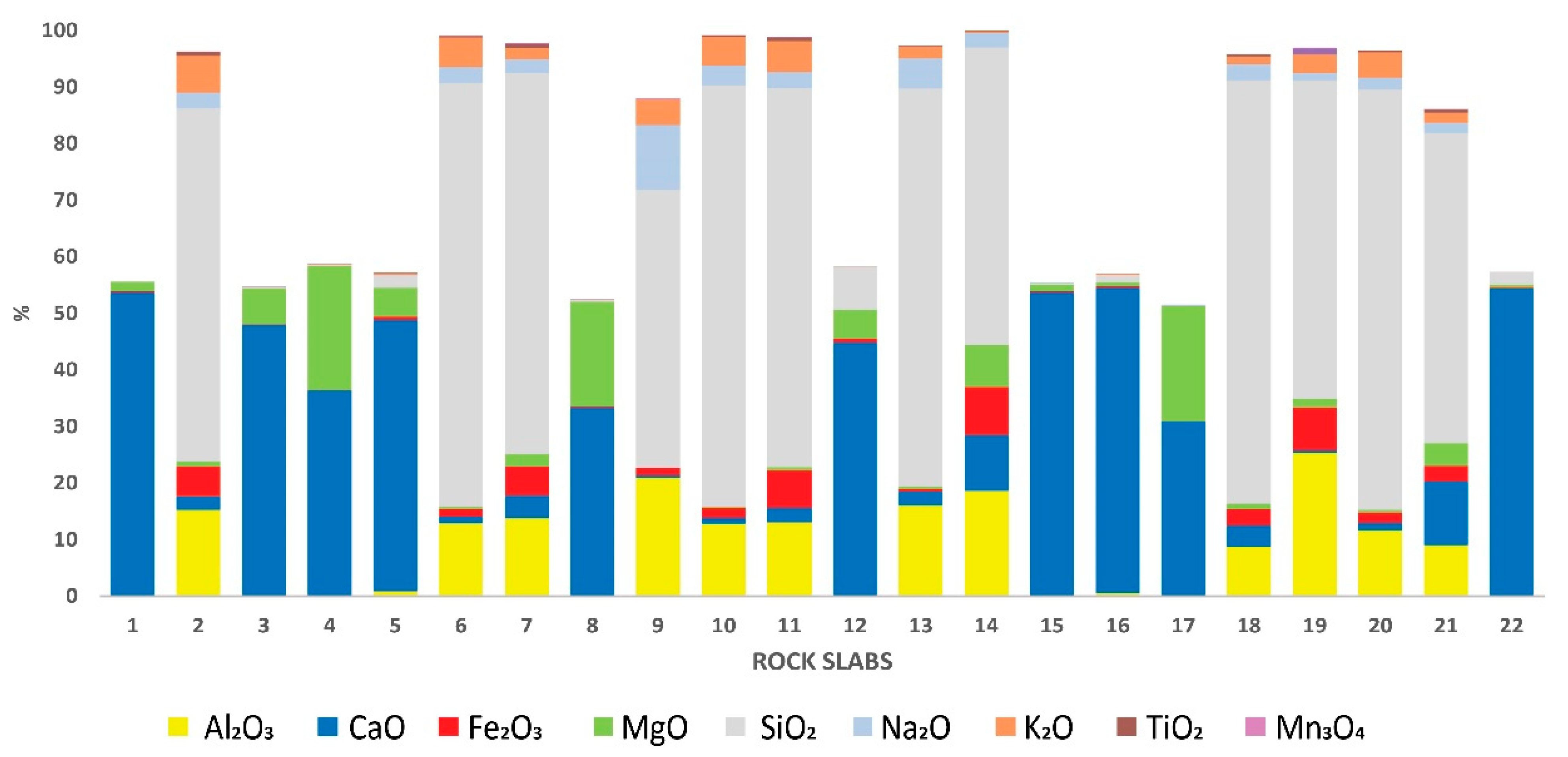
4.1. Rock Slab Chemical Composition

Whole-rock geochemical data for all slabs is given in Figure 3.

The marble slabs are mainly composed of CaO (30.9 to 54.2%) and MgO (0.56 to 22%), with lesser SiO₂ (<7.61%), Fe₂O₃ (<0.69%) and Al₂O₃ (<0.92%) (Figure 3).

For the plutonic rocks (slabs 2, 6, 7, 9, 10, 11, 13, 14, 18, 19, 20, 21), SiO₂ is the dominant chemical component and ranges from 49.02 to 74.8%. Significant other major element concentrations include Al₂O₃ (8.73 to 25.5%), CaO (0.27 to 11.2%), Fe₂O₃ (0.59 to 8.43%), Na₂O (1.22 to 11.14%) and K₂O (0.24 to 6.44%).

The marble slab samples plot into two main groups on the CaO–MgO–Fe₂O₃ ternary diagram (Figure 4a) and are split by their relative CaO and MgO content. Seven samples are dominated by CaO (>44.7%) with lesser MgO (<6.31%) and are classified as ‘marble’. Three samples are classified as ‘Mg-marble’ (MgO > 18.5%; CaO < 36.6%).

The plutonic rocks are subdivided into five distinct lithologies based on the TAS diagram: granite (slabs 6,10,13,18, 20), granodiorite (slab 7), quartz monzonite (slabs 2, 11), gabbroic diorite (slabs 14, 19, 21) and foidolite (slab 9) (Figure 4b).

The resulting lithogeochemical log for the rock slab pseudostratigraphy based on whole-rock geochemical data is shown in Figure 2b.

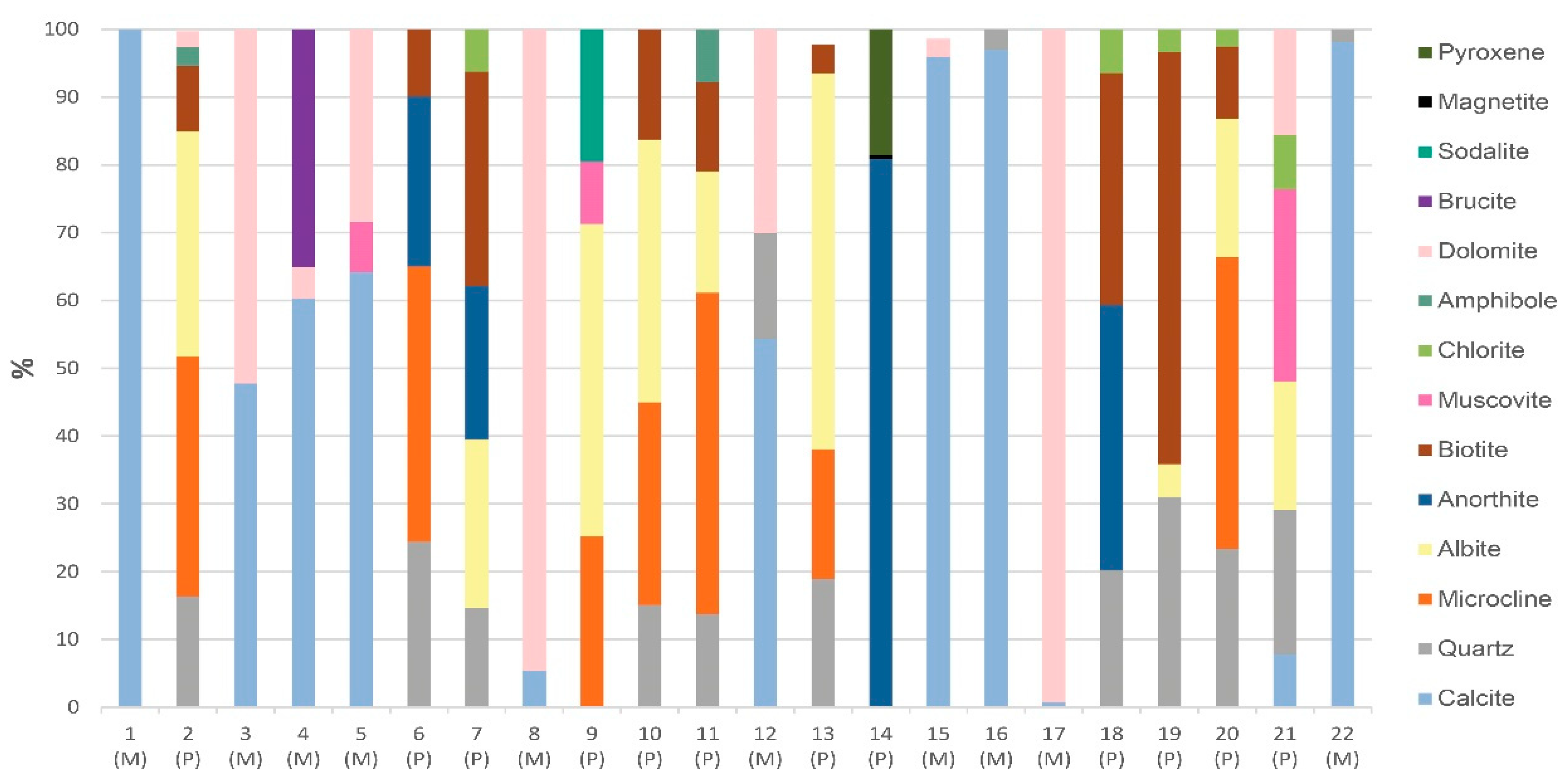
4.2. Rock Slab Mineralogical Composition

Results of XRD analysis are presented in Figure 5.

The marble slabs are dominated either by calcite or dolomite, which are the only carbonate phases present. Slabs 1, 4, 5, 12, 15, 16, 22 are calcite dominated, with 60–98% modal abundance. Slabs 3, 8, 17 are dominated by dolomite (52–99%). Slab 4 comprises ~35% brucite and is otherwise dominated by calcite (~60%) with minor dolomite (~5%). Minor mineral phases in the marble slabs are muscovite (<~7%) and quartz (<3%).

The main rock-forming minerals in plutonic rocks include quartz (15–31%), microcline (0–47%), albite (0–55%) and anorthite (0–81%). Biotite is found in the majority of the plutonic samples and is of highest abundance in slabs 7 (32%), 18 (34%) and 19 (61%). Other micas include muscovite (<28%) and chlorite (<8%). Sodalite (foid) constitutes 20% of slab 9. Pyroxene and magnetite are restricted to slab 14, and amphibole to slabs 2 and 12.

It is important to clarify that as conventional XRD is a semiquantitative technique that these mineral abundances should be considered as semiquantitative with errors of ±3%. There are also inherent complexities in the quantification of mica minerals (muscovite, chlorite, and biotite) which results in overestimation due to the preferred orientation effects. This preferred orientation is a common effect for minerals that have platy crystallites when the sample is prepared using the back-packed technique for conventional XRD analysis.

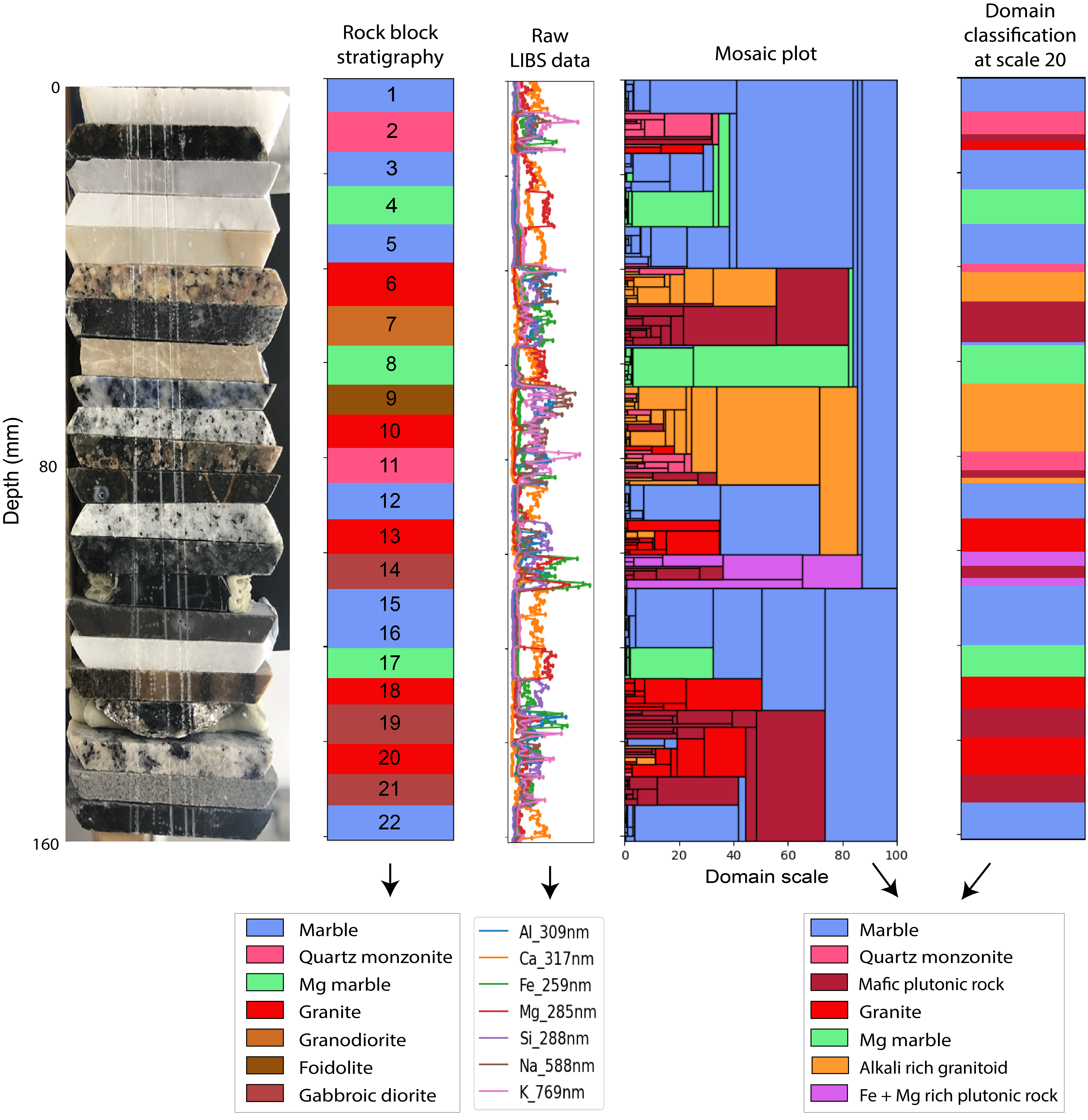
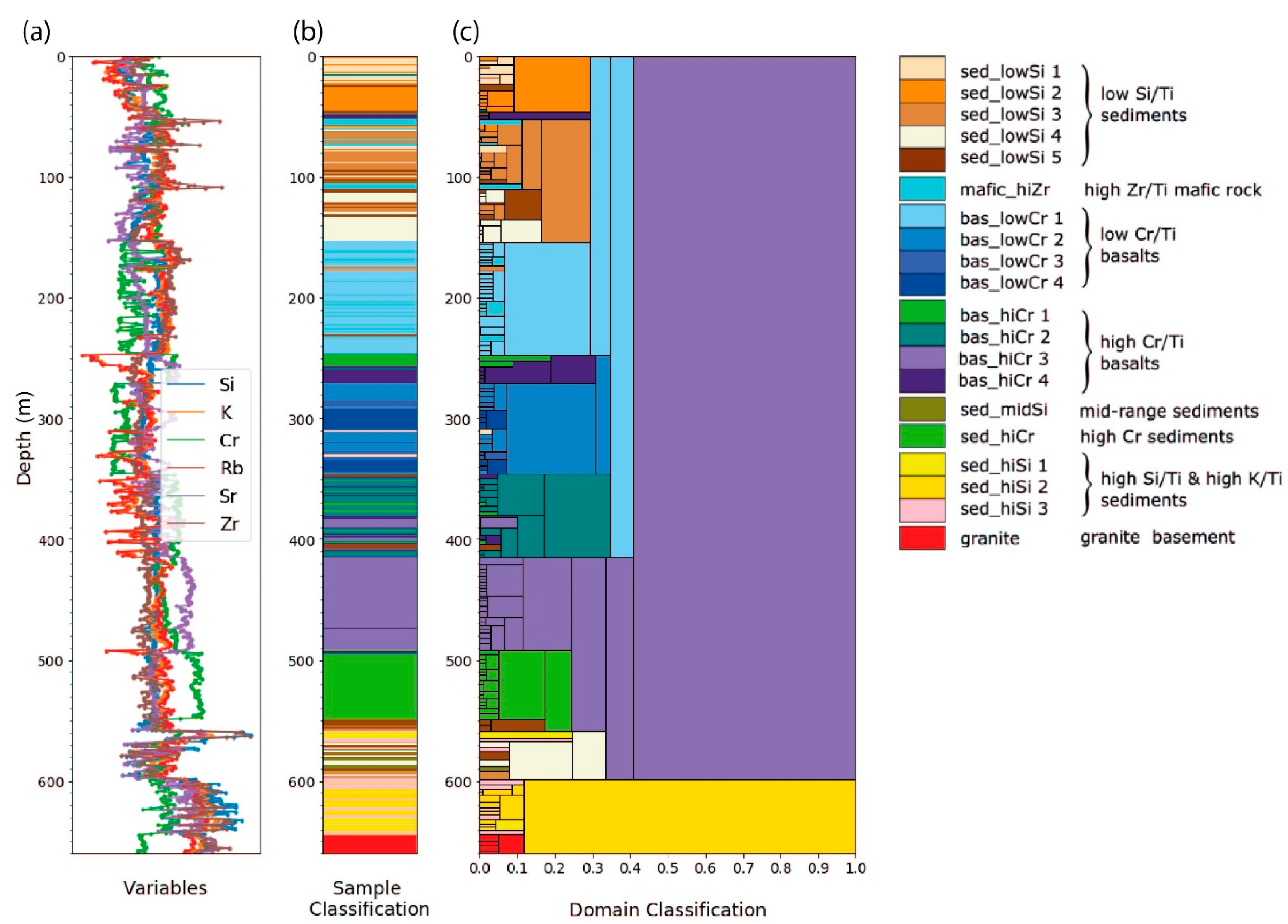
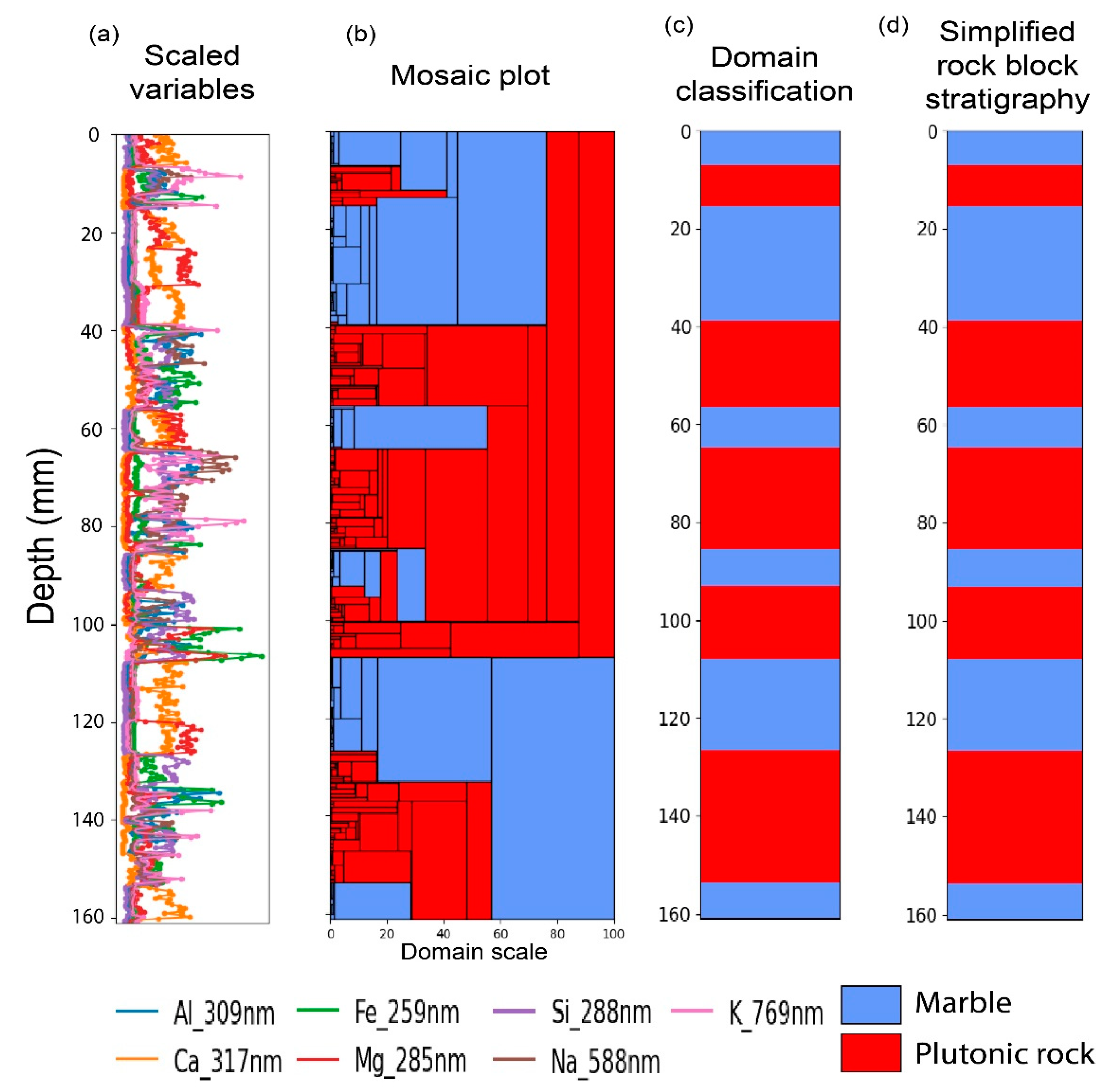
4.3. Mosaic Plots and Pseudologs

4.3.1. k = 2 Clustering

K-means clustering with k = 2 was undertaken to represent a simplified lithological stratigraphy of the two known rock types, marble and plutonic rocks. The simplified two rock type stratigraphy is based on whole-rock geochemical data (Figure 4) and visual inspection of the slab mineralogy. Slabs 1, 3, 4, 5, 8, 12, 15, 16, 17, and 22 were classified as marble, and slabs 2, 6, 7, 9, 10, 11, 13, 14, 18, 19, 20 and 21 as plutonic. K-means clustering was applied on raw LIBS data using the peak areas from the major emission lines for seven major chemical elements (Al 309 nm, Ca 317 nm, Fe 259 nm, Mg 285 nm, Si 288 nm, Na 588 nm and K 769 nm) (Figure 6a). Those same elements were input into the Data Mosaic multivariate wavelet tessellation for boundary detection, and the units identified by the wavelet tessellation were classified based on the clustering results (Figure 6b).

At domain scales from 0 to ~15, a pseudolog showing only the domain classification boundaries from the mosaic plot matches well with the geological log (compare Figure 6c to Figure 6d). In this domain classification pseudolog, the blue blocks correspond to areas of chemistry dominated by Ca and Mg, and the lack of variation in chemistry across individual slabs is evidenced by the relatively few boundaries detected by the wavelet tessellation in those regions (Figure 6b). The blue regions match well with the marble in the rock slab stratigraphy and are therefore able to be labelled as such (Figure 6c,d). Within the red blocks in the pseudolog, the chemistry is highly variable, and this is reflected in the many small-scale boundaries detected by the wavelet tessellation in those region (Figure 6b). These blocks match well with the plutonic slabs in the rock slab stratigraphy and are therefore labelled plutonic rocks (Figure 6c,d).

Comparison between the mosaic plot (Figure 6b) and the input data (Figure 6a) provides a visualization of how the boundary locations are related to the signals input into the tessellation. Boundaries between marble and plutonic rocks are controlled by the strong negative correlation between Ca and Mg, mostly present in marble slabs, and Si, Al, K, Na, Mg and Fe, mainly found within plutonic samples. The multivariate nature of these boundaries accounts for their strength in the multiscale domain plot, in which they extend to the higher domain scales (>30) (Figure 6b). Boundaries between slabs of same lithology can also be observed along the input data, and this is reflected in the multiscale domain plot. For instance, among plutonic slabs at depth = 100 mm a Si, Al and Na rich slab is in contact with a Fe and Mg dominated slab evidenced by the strong (scale ~90) boundary detected by the tessellation, and around 30 mm depth a Mg rich marble slab is adjacent to relatively Mg poorer marble slab which is shown by the weaker boundary of scale ~30. The relative strength of 100 mm and 30 mm boundaries is related to the multivariate, and univariate nature. While the classification here follows a k = 2 clustering analysis and no further classifications are made at those points, the wavelet tessellation method clearly identifies those boundaries, indicating that there is a change in sample chemistry and that perhaps a classification scheme with more clusters (k > 2) should be pursued to better describe the stratigraphy.

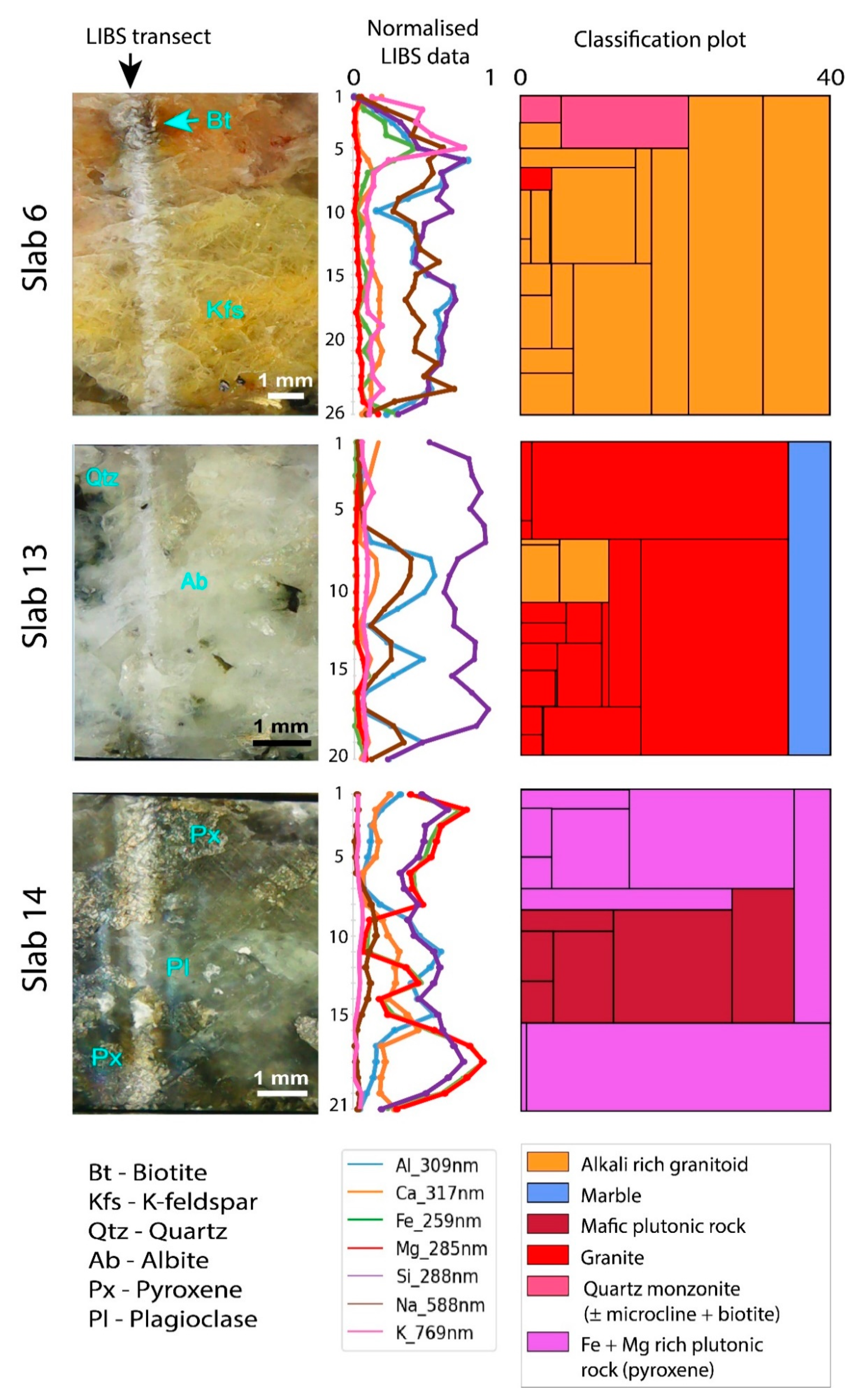
4.3.2. k = 7 Clustering

Seven domain clustering was done to assess the ability of the wavelet tessellation method to discriminate between the seven sublithologies within the sample set as identified from whole-rock geochemistry and rock-discriminant plots: marble (slabs 1, 3, 5, 12, 15, 16, 22), Mg-marble (slabs 4, 8, 17), granite (slabs 6, 10, 13, 18, 20), gabbroic diorite (slabs 14, 19, 21), quartz monzonite (slabs, 2, 11), granodiorite (slab 7), and foidolite (slab 9). Raw LIBS data of the same seven major rock-forming elements (Al, Ca, Fe, Mg, Si, Na and K) as applied to the two-domain analysis were used in the seven-domain analysis (Figure 7a) and applied to wavelet tessellation. The resultant mosaic plot produced using wavelet tessellation and k = 7 clustering analysis is shown in Figure 7b.

A domain classification pseudolog that is most similar to the rock-block stratigraphy defined from the whole-rock geochemical data occurs at a domain scale of 20 at domain scale 20 (Figure 7c,d, also see Figure 2b). This domain scale captures the boundaries of some slabs that are well defined from domain scales of 0 to ~80 (e.g., boundaries of slabs 7, 8 and 9). However, at domain scales higher than 30 the mosaic plot starts to show classifications that are not related to the composition and distribution (spacing) of the slabs (Figure 7d). Conversely, some classifications at domain scale 20 and lower show more variations than are observed in the rock-block stratigraphy (intradomain classifications), which may be attributed to smaller scale features of individual rock slabs (e.g., mineralogical variation).

Of the 22 rock-slabs, 16 were similarly classified and with boundaries almost identical to the rock block stratigraphy (compare Figure 7c,d). Marble and Mg-marble sublithology slabs were remarkably well classified with clearly defined boundaries. The only exception is the contact between slabs 7 (granodiorite) and 8 (Mg-marble). The plutonic slabs are mineralogically, and therefore geochemically, more complex than the marble slabs. This is reflected in the scaled variables (Figure 7a), in the classified mosaic plot (Figure 7b) and in the domain classification pseudolog as multiple classifications being identified within a single plutonic rock slab (e.g., Figure 7c, slabs 2, 11 and 14).

The classification of marble is representative of portions relatively rich in Ca with lesser Mg and low Al, Fe, Si, Na, and K counts. Mg-marble classification is also characterised by high Mg and Ca counts in relation to Al, Fe, Si, Na, and K counts, however Mg counts are always dominant.

The quartz monzonite classification correlates with the quartz monzonite slabs (2 and 11), but also occurs as part of the granite slab 6. Pairing the mosaic plot to the scaled variables, it is noticeable that quartz monzonite classification is associated to high K counts. The alkali-rich granitoid classification is characterised by relatively high K, Na, Al and Si high counts over low Fe, Mg and Ca counts and in the mosaic plot corresponds to slabs 9, 10 and 6 and parts of slabs 20, 13 and 11. The granite classification in the mosaic plot mainly corresponds to slabs 13, 18, and 20, and to a lesser extent parts of slabs 2, 6 and 11. The granite classification shows a similar geochemical signature to alkali-rich granitoid but has relatively higher Si counts.

The mafic plutonic rock classification corresponds mostly to Slab 7 (granodiorite), parts of gabbroic diorite slabs (14, 19, and 21), and minor parts of quartz monzonite slabs 2 and 11. The mafic plutonic rock classification is associated with relatively high Fe and often Al counts as well as variable K and Mg counts. The Fe and Mg rich plutonic rock classification applies to slab 14, which exhibits the highest Fe counts followed closed by Mg and less obviously by Si.

5. Discussion

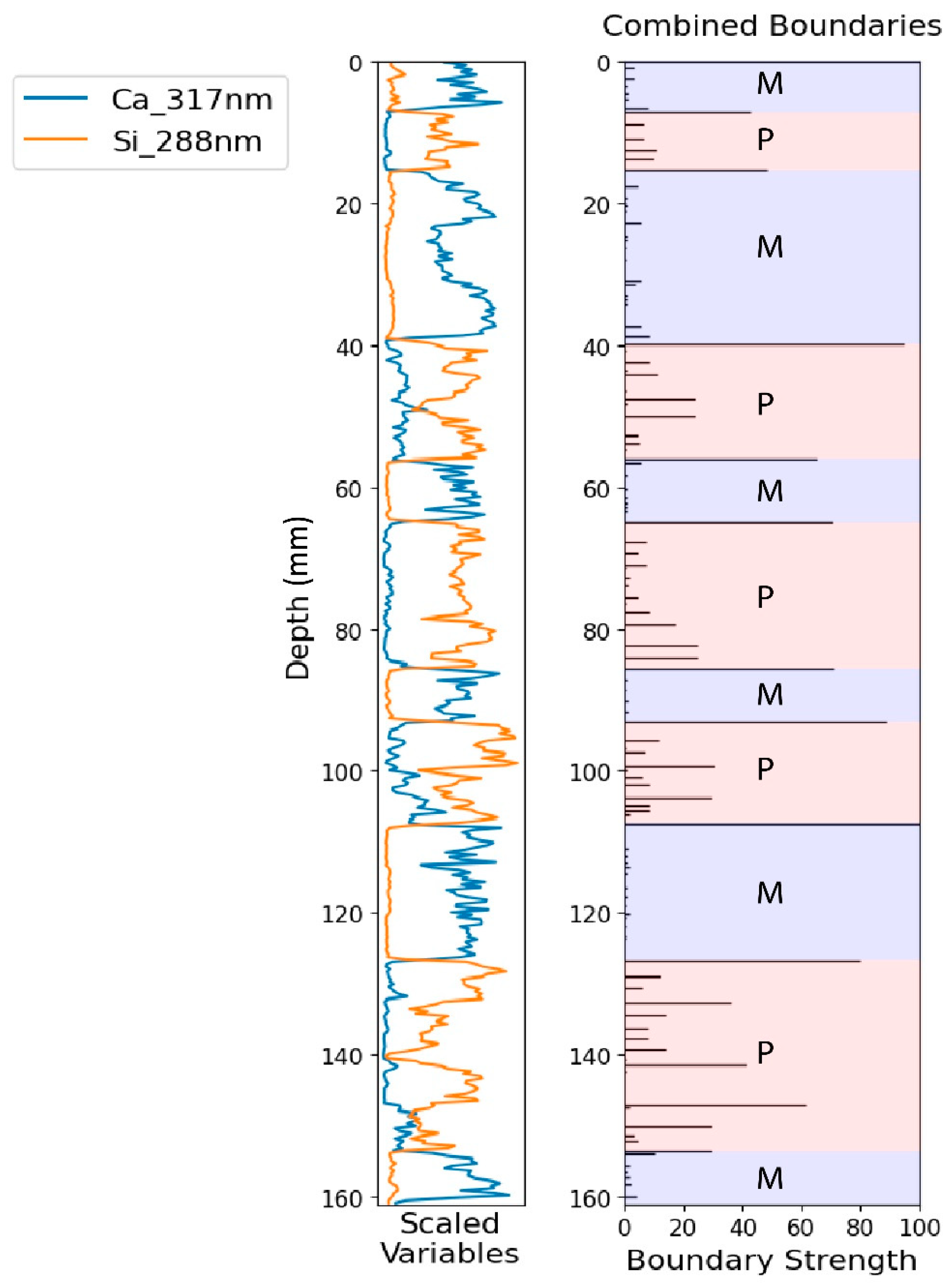
5.1. Assigning Pseudostratigraphy

Assigning pseudostratigraphy for the k = 2 classification was relatively simple as plutonic rocks (mainly granitoids) and marble are chemically distinct. The strong negative correlation between Ca and Si, mainly found within marble and plutonic samples respectively, drives the classification and detection of the main boundaries between the two rock types (Figure 8). The strongest boundaries are multivariate boundaries, in this case relative to correlated sharp variations on Si and Ca signals.

The mosaic plot generated by applying the wavelet tessellation method on LIBS data (Figure 6b) closely relates to the two-lithology simplified rock-block stratigraphy (Figure 6d). Due to its multiscale nature, the mosaic plot provides more detail in a 2D visualization than a conventional stratigraphic column. Simplifying stratigraphy to larger scale domains would be useful for very large-scale interpretation (e.g., building a regional 3D geological model). However, it is not suitable for detailed geological interpretations and lithogeochemical analysis, as the domain detection by wavelet tessellation indicates that there is greater complexity in the system, mainly within plutonic rock slabs, that cannot be fully described by two classifications (Figure 6b and Figure 8). To investigate this further, k = 7 clustering was performed.

Each of the seven coloured classifications (Figure 7b,c) corresponds to a characteristic chemistry. Therefore, each of these coloured classifications can be assigned a lithological description based on the characteristic chemistry of each other (k = 7 clustering section), and, ultimately be tested by comparing it to whole rock geochemical (XRF) and mineralogical (XRD) data. Classifications from domain scale 0 to 30 (Figure 7b) display geological meaning. The pseudolog of the classification boundaries generated at domain scale 20 is the closest match in slab divisions to the known stratigraphy (Figure 7d). It also shows finer scale boundaries within the stratigraphy. Both marble and Mg-rich marble rock-slabs are well classified and delimited in the pseudolog (Figure 7c). The exception is a small part of slab 8 (Mg-marble) that is in contact with slab 7 (granodiorite) and that is classified as marble. This misclassification is suggested to be the result of inadequate laser focusing and consequently poor plasma generation in between two slabs resulting in lower counts.

In the pseudolog of the classification boundaries, slabs 2, 6 and 11 are partly classified as quartz monzonite (Figure 7c). The quartz monzonite classification is characterised by relatively high K counts, followed by less abundant Si, Al, Na, and Fe counts (Figure 7a,b). The dominant K-bearing mineral of slabs 2, 6 and 11 is microcline, with lesser biotite (Figure 5 and Figure 9).

The alkali-rich granitoid classification corresponds to slabs 9 and 10 and parts of slab 6 and 11. Slabs 6 and 10, which are classified mostly as alkali-rich granitoid, are slightly enriched in alkalis (K₂O + Na₂O > 8.16%) compared to slabs 13, 18 and 20, which are classified as granite (K₂O + Na₂O < 7.53%). Slab 9 (foidolite) is also classified as alkali-rich granitoid. The high Na content of slab 9 is attributed to its mineralogy being dominated by albite (46%) and sodalite (20%), which is responsible for grouping it along other high alkali granitoid.

The mafic plutonic rock classification has a signature of high Fe and Al and corresponds to slabs 19 and 21 (gabbroic diorite) and 7 (granodiorite) and smaller portions of slabs 2, 11, and 14. Slabs 7, 19, 20 and 21 contain chlorite ranging from 3 to 8% modal abundance. Slabs 7, 19 and 21 also contain biotite (10–61%). The abundances of both micas likely contribute to the mafic plutonic rock classification chemical signature.

The Fe + Mg rich plutonic rock classification applies to portions of slab 14, which exhibits the highest Fe counts of all the slabs. The XRD data shows that Slab 14 is mainly composed by plagioclase and pyroxene, with minor magnetite (Figure 5). The two discrete Fe and Mg peaks observed in slab 14 (Figure 7a) are interpreted to reflect the high pyroxene content of slab 14, while other measurements within the slab are reflective of a mixture of the bulk mineralogy.

5.2. Using Small Domain Scale for Additional Interpretation

5.2.1. Mineralogy

Due to the ability to collect very high resolution chemical data (~10 µm per spot), LIBS has been used for extremely detailed imaging systems in mineralogical and petrological studies, including analysis of individual particles, mineral grains or inclusions (inclusive of chemically zoned minerals) [7,8]. Hill et al. (2020) [4] state that, for correct classification with the Data Mosaic method, at least one pure (nonmixed) sample is required. Therefore, as each LIBS spectrum in this study corresponds to ~0.35 mm, the smallest distinctive object whose boundaries can be detected must be at least two sampling intervals in length (>~0.7 mm). For the analyses in this study, a single spot measurement (~0.35) can be interpreted as the chemical composition of a single mineral grain, rather than a mixture of different mineral grains due to their coarse grained or monomineralic/homogenous nature. Integration with fundamental petrological and mineralogical knowledge may allow inferences of mineralogy and rock texture from raw LIBS data analysis using Data Mosaic to be made.

The marble slabs used in the rock block are mostly fine-grained, monomineralic, and preserve a massive texture (Figure 2), thus relatively flat patterns for their main chemical components are observed (e.g., Ca and Mg; Figure 2, Figure 5 and Figure 6a). Conversely, the plutonic slabs preserve heterogeneous mineralogy, coarse-grained textures, and have variable chemical response in LIBS data across individual slabs (Figure 2, Figure 5 and Figure 6a), related to mineral grains big enough to be recognized directly from continuous LIBS data (Figure 9).

Comparison of the mineralogy of selected samples as taken from the analysed hand specimen and informed by XRD data with the domain (rock) classification as based on LIBS chemical data demonstrates, and the analysed hand specimen shows that mineralogy can be deduced at smaller domain scales (Figure 9). For instance, in slab 6 the region classified as quartz monzonite corresponds to an area dominated by biotite and microcline and with high K counts in the LIBS data. The smaller region classified as granite is representative of abrupt relative decrease in Al and Na and higher Si. The mineralogy of this region is not as distinctive in the hand specimen but appears to be dominated by a mixture of a quartz and K-feldspar. In slab 13, the granite classified regions are coincident with a mixed quartz ± albite mineralogy (Figure 7 and Figure 9). The region classified as alkali-rich granitoid is characterized by a relative decrease in Si and increase in Al, Na, and Ca and corresponds to one albite grain in the hand specimen (Figure 9). Slab 14 is mostly classified as Fe + Mg rich plutonic rock (Figure 7b,c and Figure 9), which is coincident with areas dominated by pyroxene grains (Figure 9). The remainder of the slab is classified as mafic plutonic rock and is characterized by variable Fe, Mg, Si, Al, and Ca and relatively low K and Na. In hand specimen, this region corresponds to a mixture of plagioclase and pyroxene (Figure 9).

5.2.2. Texture

Linking the densely spaced LIBS signal at lower domain classification with mineralogical (XRD) data can be used to provide indirect information about rock texture, namely grain size. For instance, slab 14 has a dominantly bimodal mineralogy comprising plagioclase (81%) and pyroxene (19%), both of which can be seen in the hand specimen (Figure 9). Pyroxene-dominated regions are classified as Fe + Mg rich plutonic rock over two continuous intervals that correspond to ~2.8 mm (eight LIBS spots) and ~2.35 mm (seven LIBS spots) length (Figure 9). These measurements may be considered indicative of the size of the grains. Applying the same logic to slab 6 it is possible to infer that K-feldspar crystal analysed along the transect in that rock can be as big as 5.6 mm (16 LIBS spots). In slab 13, quartz grains can reach at least 2.35 mm and albite grains 1.05 mm (Figure 9).

The inferred grain size from this analysis is considered purely indicative and is based on a limited number of examples. Limitations include not being able to account for mineral aggregates, which means the grain size approximation in this estimation is too large. The estimation also cannot account for the orientation of the grain relative to the analysed surface and therefore whether the grain is larger than the area over which it is exposed at the sample surface. In this case, the estimated grain size is too small. A more accurate estimate of grain size may be gained by a larger sample population.

Furthermore, the variations in classification at smaller domain scales will also be influenced by diversity in mineralogy and the number of clusters selected for the classification algorithm. In this study, the plutonic slabs are mineralogically diverse (Figure 5), which allows for the clear distinction between the plagioclase- versus pyroxene-dominant zones in the domain classification of slab 14, for example. However, the marble slabs, which are relatively mineralogically less diverse, show relatively lower variation in classification at smaller domain scales (Figure 6b). Therefore, clear distinctions between different grains is less obvious and it is difficult to infer grain size from the LIBS data.

5.3. Broader Implications

The combination of raw LIBS geochemical data, k-means clustering, and the wavelet tessellation method offers the possibility for rapid lithogeochemical analysis and classification with multiscale stratigraphic boundary interpretation which complements conventional geological logging.

Quantitative LIBS analysis can be performed using calibration curves derived from analysis of certified reference materials. However, the disadvantage of this technique is that reference samples should be matrix-matched, and references materials with a composition similar to unknown samples are not always available e.g., complex rocks having several mineralogical phases in a variety of concentrations [33]. Multivariate algorithms that make use of the information contained in the entire spectrum can also be applied to derive accurate geochemical compositions from geological materials [34,35]. However, although the results are frequently outstanding, the algorithms need a substantial training dataset to acquire an accurate classifier and require a long training period [36].

Integration of raw LIBS data and wavelet tessellation has the potential to be applied prior to collection of quantitative data and rapidly offer meaningful results. LIBS does not require time-consuming sample preparation and offers the possibility of standoff analyses in atmospheric conditions [15], therefore saving time on organising elaborate setups. Moreover, the wavelet tessellation method demands the input of continuous numerical values of interval or ratio scale, rather than compositional data (e.g., proportions, percentages, ppm) therefore raw LIBS data (element counts) can be applied directly to the wavelet tessellation. However, it is important to note that the methodology presented here for lithogeochemical rock-type classification, based on the application of the k-means clustering algorithm on raw LIBS data, does not substitute for traditional classification based on whole-rock geochemistry data and discriminant plots (e.g., TAS diagram, Figure 4b) or a geologist logging. Rather, the method presented here is supplementary.

Depending on the selection and number of variables, distinctive descriptive classifications can be generated. In this study, for the plutonic samples, comparison was made between a TAS classification (based on SiO₂, K₂O and Na₂O contents) and k-means clustering using Al, Ca, Fe, Mg, Si, Na, and K raw LIBS data for the generation of seven clusters (k = 7). As result of the k = 7 k-means clustering foidolite (slab 9) and granite (slabs 10 and 6) were lumped and classified as alkali-rich granitoid, and gabbroic diorite (slab 14) was partly reclassified as Fe-Mg rich plutonic rock owing to high Fe and Mg counts corresponding to the presence of pyroxene grains (Figure 9). Also, granodiorite (slab 7) is reclassified as mafic plutonic rock and grouped mainly with gabbroic diorite (slabs 19 and 21). Furthermore, fit for purpose classification schemes and workflows using the integrated LIBS and wavelet tessellation method presented here could be created to identify target lithogeochemical horizons. A similar strategy was applied by Wilde et al. (2017) [30], who undertook wavelet tessellation on downhole gamma data to target key horizons in investigating sandstone-hosted uranium deposits. The advantage of LIBS being able to analyse for elements lighter than Mg opens the possibility of using the method developed here to rapidly map out alteration halos of key enriched or depleted pathfinder elements (e.g., Na alteration haloes in IOCG systems; identification of zones of Li enrichment). Moreover, the ability to undertake simplified geological classifications (e.g., two domain clustering) can be of practical value for more regional geological understanding and/or for generation regional 3D geological models (for example). For example, Le Vaillant et al. (2017) [6] utilised wavelet tessellation for reducing the total number of geological units and identifying rocks of interest in a primarily ICP-MS (Inductively Coupled Plasma Mass Spectrometry) whole rock geochemical drill hole database from the Kevitsa Ni-Cu-(PGE) deposit as a repeatable and less subjective alternative for geological classification prior to 3D modelling.

Combining wavelet tessellation with densely spaced LIBS data enables analysis on textural and mineralogical scales (Figure 9), depending on the variability of rocks mineral composition and textures and the measurement resolution. Therefore, not only can lithological boundaries be assigned, but also mineralogical boundaries (Figure 9). The collection and use of complimentary XRD data will facilitate the creation of a specific workflow for mineralogical identification. This may be useful in cases where visual examination is difficult (e.g., planetary science; deep sea environments). The ability to collect high resolution data as scanning lines or raster grids using LIBS could also be useful in cases where visual examination is not possible (e.g., downhole geochemical analysis by LIBS–MinEx CRC Real-Time Downhole Assay project https://minexcrc.com.au/program-two-data-from-drilling/project-3-real-time-downhole-assay) (access date: 28 January 2021) or not conclusive (very fine-grained textures) for effective sampling and attenuation of effects produced by heterogenous mineralogy and textures. For future studies, mineralogy (e.g., TIMA^®, QEMSCAN^®) could be used as a complimentary analytical technique for textural and mineralogical characterisation as well as validation of mineralogy interpreted from the LIBS data and wavelet tessellation analysis. Mineral interpretation could also be attempted from bigger datasets and samples including from several transect measurements along the same target.

The mosaic plots generated by the wavelet tessellation method are two-dimensional, scale-space plots that by offering the possibility of observation of hierarchical boundaries over scales from local (mineralogical) through to regional (stratigraphic). For LIBS analyses on geological materials, Fabre (2020) [8] recommends several 1D lines or 2D raster grids with a spacing finely tuned to cover any heterogeneity. The results presented here could therefore be enhanced by extra transect measurements. However, limitations in comparison of LIBS spot analyses to bulk geochemical analysis needs to be recognised and considered as LIBS data is collected from the sample surface, whereas bulk analysis data is obtained from a larger volume of the same sample. The optimal number of LIBS spot analyses for any given length or volume of rocks is still unknown [8]. Developments on LIBS sampling strategies are important to the development of new workflows for lithogeochemical analyses utilising handheld equipment, drill core and downhole deployable tools, including the utilisation of the wavelet tessellation method.

6. Conclusions

Rapid and objective lithogeochemical analysis and interpretations can be made by applying raw LIBS data collected on rocks to the wavelet tessellation method with classification by k-means clustering. Pseudologs, representative of stratigraphy, can predate further analysis (quantitative) and supplement geological logging. The ability to analyse almost every element in the periodic table with limited or no sample preparation, simple setup, and the possibility of using raw data (qualitative), with no need of data filtering and extensive processing facilitates and accelerates results and the interpretations made by the method herein presented. Previous objective knowledge is demanded. Multiple variables can be integrated, and objects are delimitated by multivariate changes in continuous data (e.g., increase in Si counts followed by a decrease in Ca counts at a marble-plutonic rocks contact). Therefore, the selection of the right variables is important. An advantage of using LIBS in wavelet tessellation for lithological characterisation is that light elements (e.g., Na and Mg) can be precisely analysed by LIBS.

As the wavelet tessellation method is based on an independent classification system applied to the data, simplified classifications can be yielded (e.g., two-clustering domain) in order to upscale classifications and generate a “lumped” rock stratigraphy, which is advantageous for regional studies and generation of large-scale geological models. Likewise, detailed classifications can be applied for meticulous lithogeochemical interpretations, which might include mineralogical and textural analysis. The two-dimensional scale-space, mosaic plots with hierarchical boundaries allow observations over all scales and integration of knowledge from different scales (e.g., lithogeochemical interpretation + mineralogical and textural inferences). While, a methodology for direct comparison of LIBS characterisation to whole-rock chemical assay is unknown, the wavelet tessellation method combined with mineralogical analyses (e.g., XRD and image analysis) can assist on the development of new sampling strategies and workflows by highlighting the impact of different rock textures and compositions on streamed geochemical data. The methodology proposed in this study has potential application in scenarios where geochemical data is, can, or could be rapidly produced in future, such as in mineral exploration.

References

1. Stevens, B.; Barnes, R.; Brown, R.; Stroud, W.; Willis, I. The Willyama Supergroup in the Broken Hill and Euriowie Blocks, New South Wales. Precambrian Res. 1988, 40–41, 297–327. [Google Scholar] [CrossRef]
2. Conor, C.H.; Preiss, W.V. Understanding the 1720–1640Ma Palaeoproterozoic Willyama Supergroup, Curnamona Province, Southeastern Australia: Implications for tectonics, basin evolution and ore genesis. Precambrian Res. 2008, 166, 297–317. [Google Scholar] [CrossRef]
3. Hill, E.; Robertson, J.; Uvarova, Y. Multiscale hierarchical domaining and compression of drill hole data. Comput. Geosci. 2015, 79, 47–57. [Google Scholar] [CrossRef]
4. Hill, E.J.; Pearce, M.A.; Stromberg, J.M. Improving Automated Geological Logging of Drill Holes by Incorporating Multiscale Spatial Methods. Math. Geol. 2021, 53, 21–53. [Google Scholar] [CrossRef] [Green Version]
5. Hill, E.J.; Uvarova, Y. Identifying the nature of lithogeochemical boundaries in drill holes. J. Geochem. Explor. 2018, 184, 167–178. [Google Scholar] [CrossRef]
6. Le Vaillant, M.; Hill, J.; Barnes, S.J. Simplifying drill-hole domains for 3D geochemical modelling: An example from the Kevitsa Ni-Cu-(PGE) deposit. Ore Geol. Rev. 2017, 90, 388–398. [Google Scholar] [CrossRef]
7. Harmon, R.S.; Lawley, C.J.; Watts, J.; Harraden, C.L.; Somers, A.M.; Hark, R.R. Laser-Induced Breakdown Spectroscopy—An Emerging Analytical Tool for Mineral Exploration. Minerals 2019, 9, 718. [Google Scholar] [CrossRef] [Green Version]
8. Fabre, C. Advances in Laser-Induced Breakdown Spectroscopy analysis for geology: A critical review. Spectrochim. Acta Part B At. Spectrosc. 2020, 166, 105799. [Google Scholar] [CrossRef]
9. Kuhn, K.; Meima, J.A.; Rammlmair, D.; Ohlendorf, C. Chemical mapping of mine waste drill cores with laser-induced breakdown spectroscopy (LIBS) and energy dispersive X-ray fluorescence (EDXRF) for mineral resource exploration. J. Geochem. Explor. 2016, 161, 72–84. [Google Scholar] [CrossRef]
10. Rifai, K.; Doucet, F.; Özcan, L.; Vidal, F. LIBS core imaging at kHz speed: Paving the way for real-time geochemical applications. Spectrochim. Acta Part B At. Spectrosc. 2018, 150, 43–48. [Google Scholar] [CrossRef]
11. Cousin, A.; Sautter, V.; Payré, V.; Forni, O.; Mangold, N.; Gasnault, O.; Le Deit, L.; Johnson, J.; Maurice, S.; Salvatore, M.; et al. Classification of igneous rocks analyzed by ChemCam at Gale crater, Mars. Icarus 2017, 288, 265–283. [Google Scholar] [CrossRef]
12. Sirven, J.-B.; Sallé, B.; Mauchien, P.; Lacour, J.-L.; Maurice, S.; Manhes, G. Feasibility study of rock identification at the surface of Mars by remote laser-induced breakdown spectroscopy and three chemometric methods. J. Anal. At. Spectrom. 2007, 22, 1471–1480. [Google Scholar] [CrossRef]
13. Wiens, R.C.; Maurice, S.; Barraclough, B.; Saccoccio, M.; Barkley, W.C.; Bell, J.F.; Bender, S.; Bernardin, J.D.; Blaney, D.L.; Blank, J.; et al. The ChemCam Instrument Suite on the Mars Science Laboratory (MSL) Rover: Body Unit and Combined System Tests. Space Sci. Rev. 2012, 170, 167–227. [Google Scholar] [CrossRef]
14. Thornton, B.; Takahashi, T.; Sato, T.; Sakka, T.; Tamura, A.; Matsumoto, A.; Nozaki, T.; Ohki, T.; Ohki, K. Development of a deep-sea laser-induced breakdown spectrometer for in situ multi-element chemical analysis. Deep. Sea Res. Part I Oceanogr. Res. Pap. 2015, 95, 20–36. [Google Scholar] [CrossRef] [Green Version]
15. Cremers, D.A.; Chinni, R. Laser-Induced Breakdown Spectroscopy—Capabilities and Limitations. Appl. Spectrosc. Rev. 2009, 44, 457–506. [Google Scholar] [CrossRef]
16. Cremers, D.A.; Radziemski, L.J. Handbook of Laser-Induced Breakdown Spectroscopy; Wiley: Hoboken, NJ, USA, 2013. [Google Scholar]
17. Nicolodelli, G.; Cabral, J.; Menegatti, C.R.; Marangoni, B.; Senesi, G.S. Recent advances and future trends in LIBS applications to agricultural materials and their food derivatives: An overview of developments in the last decade (2010–2019). Part I. Soils and fertilizers. TrAC Trends Anal. Chem. 2019, 115, 70–82. [Google Scholar] [CrossRef]
18. Senesi, G.S.; Cabral, J.; Menegatti, C.R.; Marangoni, B.; Nicolodelli, G. Recent advances and future trends in LIBS applications to agricultural materials and their food derivatives: An overview of developments in the last decade (2010–2019). Part II. Crop plants and their food derivatives. TrAC Trends Anal. Chem. 2019, 118, 453–469. [Google Scholar] [CrossRef]
19. Jolivet, L.; Leprince, M.; Moncayo, S.; Sorbier, L.; Lienemann, C.-P.; Motto-Ros, V. Review of the recent advances and applications of LIBS-based imaging. Spectrochim. Acta Part B At. Spectrosc. 2019, 151, 41–53. [Google Scholar] [CrossRef]
20. Sanghapi, H.K.; Ayyalasomayajula, K.K.; Yueh, F.Y.; Singh, J.P.; McIntyre, D.L.; Jain, J.C.; Nakano, J. Analysis of slags using laser-induced breakdown spectroscopy. Spectrochim. Acta Part B At. Spectrosc. 2016, 115, 40–45. [Google Scholar] [CrossRef] [Green Version]
21. Khajehzadeh, N.; Haavisto, O.; Koresaar, L. On-stream and quantitative mineral identification of tailing slurries using LIBS technique. Miner. Eng. 2016, 98, 101–109. [Google Scholar] [CrossRef]
22. Rifai, K.; Özcan, L.; Doucet, F.; Vidal, F. Quantification of copper, nickel and other elements in copper-nickel ore samples using laser-induced breakdown spectroscopy. Spectrochim. Acta Part B At. Spectrosc. 2020, 165, 105766. [Google Scholar] [CrossRef]
23. Singh, J.P.; Almirall, J.R.; Sabsabi, M.; Miziolek, A.W. Laser-induced breakdown spectroscopy (LIBS). Anal. Bioanal. Chem. 2011, 400, 3191–3192. [Google Scholar] [CrossRef] [Green Version]
24. Guo, J.; Lu, Y.; Cheng, K.; Song, J.; Ye, W.; Li, N.; Zheng, R. Development of a compact underwater laser-induced breakdown spectroscopy (LIBS) system and preliminary results in sea trials. Appl. Opt. 2017, 56, 8196–8200. [Google Scholar] [CrossRef]
25. Gómez-Nubla, L.; Aramendia, J.; De Vallejuelo, S.F.-O.; Madariaga, J.M. Analytical methodology to elemental quantification of weathered terrestrial analogues to meteorites using a portable Laser-Induced Breakdown Spectroscopy (LIBS) instrument and Partial Least Squares (PLS) as multivariate calibration technique. Microchem. J. 2018, 137, 392–401. [Google Scholar] [CrossRef] [Green Version]
26. Witkin, A.P. Scale-space filtering. Read. Comput. Vision 1987, 2, 329–332. [Google Scholar]
27. Arabjamaloei, R.; Edalatkha, S.; Jamshidi, E.; Nabaei, M.; Beidokhti, M.; Azad, M. Exact Lithologic Boundary Detection Based on Wavelet Transform Analysis and Real-Time Investigation of Facies Discontinuities Using Drilling Data. Pet. Sci. Technol. 2011, 29, 569–578. [Google Scholar] [CrossRef]
28. Cooper, G.R.J.; Cowan, D.R. Blocking geophysical borehole log data using the continuous wavelet transform. Explor. Geophys. 2009, 40, 233–236. [Google Scholar] [CrossRef]
29. Perez-Muñoz, T.; Velascohernandez, J.X.; Hernandez-Martinez, E. Wavelet transform analysis for lithological characteristics identification in siliciclastic oil fields. J. Appl. Geophys. 2013, 98, 298–308. [Google Scholar] [CrossRef]
30. Wilde, A.; Hill, E.J.; Schmid, S.; Taylor, W.R. Wavelet Tessellation and its Application to Downhole Gamma Data from the Manyingee & Bigrlyi Sandstone-Hosted Uranium Deposits. AIG J. 2017, N2017-001, 1–11. [Google Scholar]
31. Templ, M.; Filzmoser, P.; Reimann, C. Cluster analysis applied to regional geochemical data: Problems and pos-sibilities. Appl. Geochem. 2008, 23, 2198–2213. [Google Scholar] [CrossRef]
32. Middlemost, E.A. Naming materials in the magma/igneous rock system. Earth-Sci. Rev. 1994, 37, 215–224. [Google Scholar] [CrossRef]
33. Fahad, M.; Farooq, Z.; Abrar, M. Comparative study of calibration-free laser-induced breakdown spectroscopy methods for quantitative elemental analysis of quartz-bearing limestone. Appl. Opt. 2019, 58, 3501–3508. [Google Scholar] [CrossRef]
34. Anderson, R.B.; Clegg, S.M.; Frydenvang, J.; Wiens, R.C.; McLennan, S.; Morris, R.V.; Ehlmann, B.; Dyar, M.D. Improved accuracy in quantitative laser-induced breakdown spectroscopy using sub-models. Spectrochim. Acta Part B At. Spectrosc. 2017, 129, 49–57. [Google Scholar] [CrossRef]
35. Clegg, S.M.; Sklute, E.; Dyar, M.D.; Barefield, J.E.; Wiens, R.C. Multivariate analysis of remote laser-induced breakdown spectroscopy spectra using partial least squares, principal component analysis, and related techniques. Spectrochim. Acta Part B At. Spectrosc. 2009, 64, 79–88. [Google Scholar] [CrossRef]
36. Shah, S.K.H.; Iqbal, J.; Ahmad, P.; Khandaker, M.U.; Haq, S.; Naeem, M. Laser induced breakdown spectroscopy methods and applications: A comprehensive review. Radiat. Phys. Chem. 2020, 170, 108666. [Google Scholar] [CrossRef]
Figure 1. Example of input data and resulting plots generated from using the wavelet tessellation method to interpret a multielement geochemical dataset after Hill et al. (2020) [4]. Plots were produced using the Data Mosaic online web application (https://datamosaic.geoanalytics.group/) (access date: 28 January 2021). (a) Plots of scaled signals of elements of interest; (b) sample classification pseudolog at scale 0.0, samples are coloured by lithogeochemical classification at lowest boundary strength (domain classification) equals 0.0; (c) multiscale domains coloured by lithogeochemical classification.
Minerals 11 00312 g001
Figure 2. Rock block assembled for this study. (a) Rock block of approximately 16 cm length, composed of 22 distinct rock slabs; (b) lithogeochemical log of the rock block. Lithologies assigned according to CaO-MgO-Fe2O3 (for marbles) and total alkali versus silica (for igneous plutonic rocks) discrimination diagrams and using whole-rock geochemical data.
Minerals 11 00312 g002
Figure 3. Results of whole-rock geochemical analysis for the 22 rock slabs in oxides. Samples dominated by CaO (blue colour) are marbles. Samples dominated by SiO2 (grey colour) are plutonic rocks (mainly granitoids). Detail on rock slab lithology is given in Figure 4. (Note: Loss on ignition (LOI) is not reported here. It is expected that carbonate-dominated samples will have high LOI (~40–50%) due to CO2 generation during heating.
Minerals 11 00312 g003
Figure 4. Lithological classification of marble and plutonic slabs based on laboratory whole rock geochemical data. (a) CaO-MgO-Fe2O3 ternary diagram used to classify marble slabs. (b) Total alkali versus silica diagram (TAS) [32] used to classify the plutonic rocks. Numbers shown next to sample points correspond to the rock slab number shown in Figure 2a. Sample colours legend is shown in Figure 2c.
Minerals 11 00312 g004
Figure 5. X-ray diffraction (XRD) results for samples used in this study; (M) marble, (P) plutonic.
Minerals 11 00312 g005
Figure 6. Results for k = 2 cluster analysis of raw laser-induced breakdown spectroscopy (LIBS) data based on classification by k-means clustering. (a) Scaled variables; (b) multiscale mosaic plot showing the boundaries detected by wavelet tessellation from raw LIBS data with the k = 2 cluster classification applied; (c) simplified marble vs. plutonic rocks block stratigraphy based on laboratory whole-rock geochemistry; (d) pseudolog of the domain classification at domain scale = 0.
Minerals 11 00312 g006
Figure 7. Results for seven domain analysis of raw LIBS data based on classification by k-means clustering. (a) Scaled variables; (b) multiscale mosaic plot for seven domains produced by wavelet tessellation of raw LIBS data block stratigraphy with rock slab numbers; (c) domain classification pseudolog for seven domain classification at domain scale 20; (d) Rock block stratigraphy with rock slab numbers.
Minerals 11 00312 g007
Figure 8. Ca (317 nm) and Si (288 nm) LIBS data combined boundaries generated through wavelet tessellation. Note that superimposed sharp variations on Ca and Si counts are related to the strongest boundaries (multivariate boundaries) and the presence of intraslab boundaries suggests the possibility of refined classifications, mainly relative to plutonic slabs. (M = marble, P = plutonic; classification from whole rock geochemistry data, Figure 4).
Minerals 11 00312 g008
Figure 9. Detailed examination of slabs 6, 13, 14 and their classified data mosaic plots for mineralogical and textural analysis showing the hand specimen (left), scaled variables (middle) and seven-domain analysis multiscale mosaic classifications for domain scale 0–40 (right). LIBS data were normalised from 0 to 1. Each point along the scaled variables represents one LIBS measurement, corresponding to ~0.35 mm distance.
Minerals 11 00312 g009
Publisher’s Note: MDPI stays neutral with regard to jurisdictional claims in published maps and institutional affiliations.