Quantifying the Distribution Characteristics of Geochemical Elements and Identifying Their Associations in Southwestern Fujian Province, China


1
College of Earth Science, Chengdu University of Technology, Chengdu 610059, China
2
State Key Laboratory of Geological Processes and Mineral Resources, China University of Geosciences, Wuhan 430074, China
*
Author to whom correspondence should be addressed.
Minerals 2020, 10(2), 183; https://doi.org/10.3390/min10020183
Submission received: 29 December 2019
/
Revised: 28 January 2020
/
Accepted: 30 January 2020
/
Published: 18 February 2020
(This article belongs to the Section Mineral Deposits)
Abstract
:The distribution of geochemical elements in the surficial media is the end product of geochemical dispersion under complex geological conditions. This study explored the frequency and spatial distribution characteristics of geochemical elements and their associations. It quantifies the frequency distribution via mean, variance, skewness and kurtosis, followed by measuring the spatial distribution characteristics (i.e., spatial autocorrelation, heterogeneity and self-similarity) via semivariogram, q-statistic and multifractal spectrum, and further identify the elemental associations based on these distribution parameters using hierarchical clustering. A criterion was defined to identify the importance of parameters in the clustering procedure. A case study processing a geochemical dataset of stream sediment samples collected in southwestern Fujian province of China was carried out to illustrate and validate the procedure. The results indicate that studies of the frequency and spatial distribution characteristics of geochemical elements can enhance the knowledge of geochemical dispersions. The associations identified based on the frequency and spatial distribution parameters are different from those obtained by conventional cluster analysis. Spatial distribution characteristics cannot be neglected when investigating the distribution patterns of geochemical elements and their associations. The findings can enhance the knowledge of the geochemical dispersion in the study area and might benefit the following-up mineral exploration.
1. Introduction
The distribution of geochemical elements in the surficial media is the end product of various geological processes and anthropogenic activities [1]. These geological processes, including the primary and secondary ones, can occur at a wide range of spatial and temporal scales, and are affected by the local physical-chemical conditions (e.g., temperature, pressure, fluid, etc.). The geochemical diffusion of elements can involve different migration mechanisms, driving factors, etc. These processes together result in the complex distribution patterns of geochemical elements in the surface and subsurface media. Exploring the spatial and frequency distribution characteristics of geochemical elements and their associations can help to enhance the knowledge of the underlying geological processes [2,3]. Moreover, this is an essential step for identifying anomalous geochemical patterns associated with hidden mineralization [4,5].
The distribution characteristics of geochemical elements are usually quantified in terms of frequency distribution, spatial distribution and elemental associations. Studies show that trace elements usually do not follow normal or lognormal distribution, but distribute with a heavy and long tail that can be modeled by a Pareto distribution [6,7,8,9,10]. Such a scaling property boosted the development of fractal models to characterize the frequency distribution of geochemical element concentrations, such as the concentration-area model [7]. The spatial distribution of geochemical elements in the surficial media can be manifested through scale-dependence and scale-independence [11]. Spatial autocorrelation and heterogeneity are two general properties of geospatial data, which means different characteristics can be observed at different scales [12]. Spatial autocorrelation, termed Tobler’s law, states that everything is related to everything else, but near things are more related than distant things [13]. This law lays the foundation of the regionalized variable theory for geostatistics [14,15,16]. Spatial heterogeneity of some quantity, or non-stationarity, refers to the uneven distribution of the quantity within a given area [17]. In exploration geochemistry, the commonly used criterion “mean ± k standard deviations” has been demonstrated to be limited in identifying local weak anomalies. One of the most important reasons lies in that the approach fails to allow for the spatial heterogeneity of geochemical patterns in the surficial media [18]. Many models accommodating spatial heterogeneity have been proposed, such as local Reed–Xiaoli (RX), local enrichment index, local gap statistic, etc., and their improved performance for identifying geochemical anomalies from the background have been validated by case studies [18,19,20]. Scale-independent variation, also termed self-similarity, refers to similar processes or patterns of geoscientific phenomena which can be observed at different scales, forming the foundation of fractal and multifractal theory [21]. Studies have revealed that the spatial distribution of geochemical elements is also self-similar but holds in a statistical sense and is constrained within a certain range of scales [22,23]. Multifractal spectrum and generalized fractal dimension are widely used tools to explore the spatially scale-independent property of the quantity of interest, and has been applied in geology, ecology, environment and climate sciences [24,25,26]. Note that the scale-independent components of the geospatial variables can be derived at the target scale using fractal or multifractal theory, but within a certain scale, the scale-dependent variation can still exist. Therefore, all the properties, including spatial autocorrelation, heterogeneity and self-similarity, should be considered when exploring the spatial distribution patterns of geochemical elements.
Elements with similar geochemical mobility tend to occur together during the primary and secondary dispersion processes, and hence exhibit similar distribution patterns [27]. The geochemical associations usually vary a lot, since the mobility of the geochemical elements can vary with changes in environmental conditions. Some elements commonly coexisting during diagenesis may part company during surficial weathering and sedimentation. For example, lead and zinc usually coexist during the formation of sulfide ore deposits, but zinc tends to migrate into solutions by the oxidation of sphalerite and separate from lead in the surficial environment [27]. Association of geochemical elements can be indicative of certain geochemical processes [3,28]. It has been demonstrated that indicative ability of pathfinder element association for buried ore deposits far outweighs that of single element [29]. For geochemical exploration, methods used for exploring elemental associations vary from geologically to numerically. For example, Zuo [30] summarized that there are three approaches to identify element associations for a specific type of mineral deposit: geology-based, multivariate statistics-based and spatial distribution-based methods. By collecting ore or rock samples, the association can be inferred through the stoichiometry of ore-forming minerals [31,32,33,34,35]. Such investigations on a certain type of mineral deposit have been summarized as exploration geochemical models and have been used in turn to find potential deposits of that type in other areas [31,36,37,38]. Characteristic zonation of mineralization-related minerals/elements is a widely used tool for locating buried mineralization [39,40]. For instance, polymetallic mineralization associated with the granites of Cornwall, Southwest England, shows that the ore mineral zonation progresses from an early oxide-dominated assemblage (cassiterite, wolframite, etc.) to a later sulfide assemblage (chalcopyrite, sphalerite, galena and chlorite). The zonation pattern away from the granite body is evident both vertically and laterally, which can be used for vectoring into the hidden ore body [41]. But for geochemical elements in the surficial media, such as stream sediments, lake sediments, till and soil, the association of elements may be only partially in agreement with that determined from ore rock samples due to diverse secondary processes involved in the formation of geochemical patterns. It is a great challenge or even impossible for experts to explore the association between elements by quantitatively modeling all the geological processes affecting the dispersion of geochemical elements. Statistical analysis of geochemical datasets is a more straightforward alternative to determine the elemental association. A variety of statistical models have been used to analyze exploration geochemical data during the past several decades [3,5,7,42,43,44,45,46,47,48,49]. Commonly used methods for determining associations of geochemical elements include multivariate statistical analysis (e.g., principal component analysis, clustering analysis, factor analysis) and visually inspecting the degree of coincidence of spatial variation patterns for different elements [19,34,40,50,51,52,53,54,55,56,57,58,59]. These statistical methods can serve as powerful tools for the interpretation of element distributions, and thereby improving our knowledge of the dispersion process of geochemical elements. However, most of these statistical approaches are based on the variance–covariance matrix of the multivariate geochemical dataset, failing to allow for the spatial structure of distribution patterns of geochemical elements. The spatial patterns of geochemical elements should provide additional information on the variations and associations of geochemical elements, which can benefit the understanding of the underlying geochemical dispersion processes.
This contribution presents a study exploring both the frequency and spatial distribution characteristics of geochemical elements, and further identify association of geochemical elements based on the distribution characteristics. A case study by quantifying the distribution characteristics of geochemical elements in stream sediment samples in southwestern Fujian province, China is presented to illustrate and validate the procedure.
2. Methods
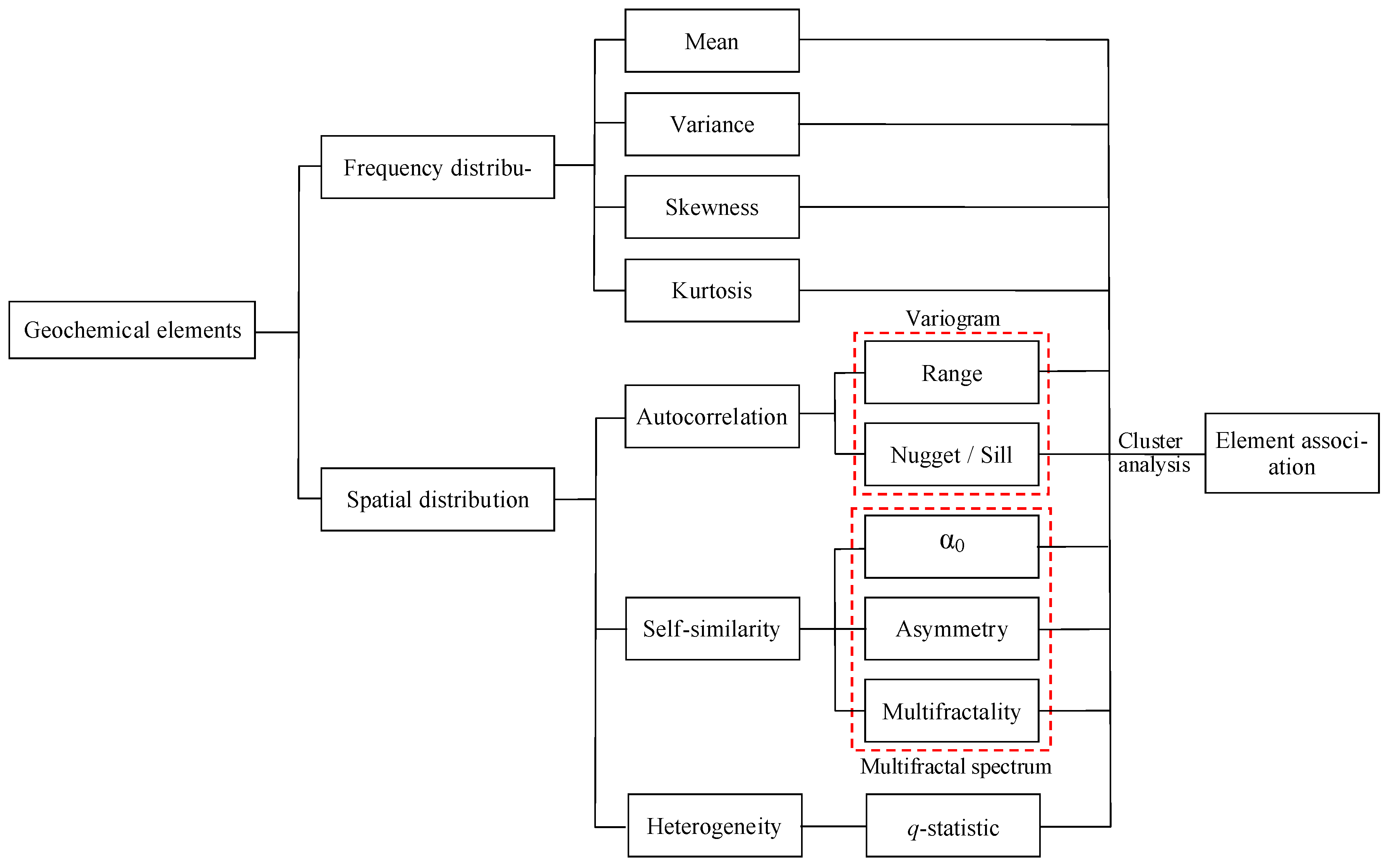
The whole workflow is presented in Figure 1. We firstly explored the frequency distribution characteristics of different geochemical elements, and then their spatial patterns from perspectives of spatial autocorrelation, self-similarity and spatial heterogeneity. Each distribution property was summarized by one or more parameter. These parameters can not only enhance the understanding of geochemical distribution, but also help determine the association of geochemical elements using clustering analysis.
2.1. Frequency Distribution
The frequency distribution of geochemical elements in rocks and other natural materials usually exhibits complicated patterns. It is usually hard to find a parametric distribution function to properly fit the distribution of sample data. Four statistics were used in this paper to parameterize the shape properties of frequency distribution of geochemical elements, i.e., mean, variance, skewness, kurtosis. The statistical mean was used to reflect the central tendency of the data in question. The variance measures how far a set of random numbers are spread out from their statistical mean. However, the variances of two variables cannot be compared in any meaningful way since they have different units. The coefficient of variation (CV), calculated as the ratio of the standard deviation to the mean, is a normalized and unit-less measure for dispersion. The skewness refers to the asymmetry of the probability distribution about its mean. Kurtosis can be used to identify whether the tails of a given distribution contain extreme values. The skewness and kurtosis are third and fourth standardized moments of the distribution, respectively, and also serve as unit-less measures. The statistics above are commonly used shape parameters to characterize the lower-order statistics of sample data.
2.2. Spatial Autocorrelation and Semivariogram
Spatial autocorrelation refers to the fact that attributes observed at nearby locations are statistically correlated, and such correlation usually decays with the separated distance. Semivariogram is a commonly used tool to measure the spatial autocorrelation. Under the intrinsic assumption of stationarity for regionalized random variable [16], semivariogram can be defined as:
where Z(x) represents regionalized random variable at location x, h is Euclidean distance separating two observations in space; E() denotes the statistical expectation. Before calculating the experimental semivariogram, normal score transform is usually performed to make the expected variance of the sample data asymptotic to unity and the mean to zero. The experimental semivariograms are usually fitted with a theoretical model, the commonly used ones including Gaussian, exponential and spherical variogram models. For the variogram models with presence of sill, two parameters are usually derived to equivalently represent the semivariogram, i.e., range and the nugget to sill ratio (or NSR). The parameter “range” measures the extent within which spatial autocorrelation occurs, and the ratio of nugget to sill indicates the degree of spatial autocorrelation [60]. Semivariogram can be also used to quantify more complicated distribution patterns of geochemical elements, such as spatial anisotropy. In such a case, an integrated semivariogram model consisting of several semivariogram models characterizing spatial dependence in different directions needs to be built. In our case, omnidirectional semivariogram will be considered and the range and NSR parameters are extracted to reflect the characteristics of spatial autocorrelation.
2.3. Scale-Independence and Multifractal Spectrum
Scale-independence has been identified to be an intrinsic property of the distribution of many physical quantities, which are thereby called multifractals [61,62]. Multifractals consist of spatially intertwined fractals, each characterized by its own singularity strength and fractal dimension [22,63,64,65]. Multifractal spectrum is a popular tool for quantifying the multifractal distribution.
Without loss of generality, let us take a 2-D distribution of some quantity (geochemical distributions of element concentrations, geophysical parameters, etc.) as an example to introduce the general procedure of multifractal analysis. Multifractal analysis is usually implemented by partitioning the measure on the 2D region and covering it with a set of boxes of fixed size. We assumed the size of each box as ε × ε, and there were Nε boxes in total. We further assumed a measure μi is defined on the ith small box, and this measure can be derived by [66]
where represents proportionality; αi is called the coarse Hölder exponent (also known as singularity index) and can be estimated as [61]
This expression suggests that the measure μ is a function of scale ε and possessing scale- invariant property. For 2-D geochemical distribution, the case of α − 2 < 0 indicates an enriched local pattern, α − 2 > 0 represents a depletion pattern, and α − 2 = 0 denotes a nonsingular local pattern. Moreover, the larger the absolute of difference |α − 2| is, the more singular (enriched or depleted) the local pattern is. A simulated example illustrating the singularity index indicating enrichment/depletion patterns was provided in Zuo et al. [67]. More details on physical properties of singularity index can be referred to Cheng [23] and Feder [62]. Evertsz and Mandelbrot [61] showed that this exponent α is usually constrained to a finite interval [αmin, αmax] for a wide range of self-similar measures. Perform the procedure over the entire 2-D region, and distribution of singularity index can be obtained. The entire set of α for Nε boxes can be divided into multiple subsets, each having the same singularity exponent value. Assuming the number of boxes with the singularity index α is Nε(α), it follows a power-law relation with the scale ε according to the multifractal theory:
If the function f(α) approaches a limit when , then [68]
This definition of f(α) suggests that the number of boxes for given α increases with the decrease in ε. The value of f(α) can be loosely interpreted as fractal dimension of the subset with the same singularity index α in the limit . For the case where , there is an increasing number of subsets, each characterized by a particular singularity index and a corresponding fractal dimension; this is the reason why the field of measure μ is called “multifractal” [61].
A graph of f(α) against α can be derived from the procedure mentioned above. This curve is referred to as multifractal spectrum of the measure of interest. This curve is a convex function and takes a shape like a parabola. Multifractal spectrum can be used to quantify multi-scale distribution structures of the measure. Cheng [66] suggested that the complexity of multifractals can be equivalently represented by a vector consisting of three parameters, i.e., (α(0), R, ∆α). α(0) is the singularity index where the fractal dimension spectrum function reaches the maximum (also known as box-counting fractal dimension); R is denoted as “asymmetry index” and usually defined as ; ∆α is calculated by [2,66]. ∆α can be used to measure multifractality. In theory, the case of ≠ 0 indicates the presence of multifractality, while = 0 represents nonfractal or monofractal [2,63,66]. The wider the range of ∆α is, the more complicated and diverse patterns can be found in the geochemical distributions. Other parameters derived from the multifractal spectrum also can be used to characterize the multifractality of the distribution [69,70]. The range of singularity index can be divided into two parts: the left half, , and the right half, . The left part corresponds to enrichment patterns, and the right part indicate depletion patterns. The asymmetry index R is defined based on these two parts. Both enrichment and depletion patterns usually coexist for geochemical distribution, but one of them dominate if the multifractal spectrum is asymmetrical. Xie and Bao [2] performed simulated experiments and the results indicate that the asymmetry index can imply whether the enrichment or depletion patterns are dominant. The case of R > 1, i.e., the entire spectrum is bent to the left, suggests that enrichment patterns are dominant, while R < 1 indicates that depletion patterns are more important.
2.4. Spatial Heterogeneity and q-Statistic
Spatial varying geological settings and geographical landscape conditions lead to the spatial heterogeneity of geochemical patterns. The presence of spatial heterogeneity indicates that different distribution patterns and element associations might exist for different local areas, thus requiring different models or distribution parameters be constructed when shifting from one location to another. Spatial heterogeneity can be divided into two types, i.e., local and stratified heterogeneity [71]. Spatial local heterogeneity refers to the case where the observation at the current location is deviated from its surrounding observations, and spatial stratified heterogeneity indicates that the variance within the stratified zones is less than that between the stratified zones. Spatial stratified heterogeneity of a variable can be measured by q-statistic [71]:
where L is the number of stratified zones by exclusively partitioning the complete region, N denotes the size of the sample, and σ2 stands for the variance of the variable. The value of the q-statistic falls within [0, 1]. The case q = 0 indicates no spatial stratified heterogeneity, while q = 1 represents perfect spatial heterogeneity [71].
2.5. Hierarchical Clustering
The statistics mentioned above can provide insights into the distribution of geochemical elements, which benefits the recognition of the underlying geological processes related to element dispersion.
Clustering geochemical elements based on these frequency and spatial distribution parameters might produce element associations different but more reliable than the correlation coefficient-based methods. Hierarchical clustering is a method which seeks to construct a hierarchy of clusters based on certain dissimilarity measures [72]. There are generally two strategies for hierarchical clustering, i.e., agglomerative and divisive clustering. The former is a “bottom-up” approach, in which each observation is firstly seen as a cluster, and pairs of clusters are gradually merged according to the dissimilarity measure. The divisive clustering is a “top-down” approach, in which all observations belong to the same cluster, and splits recursively into two parts as one moves down the hierarchy [73]. The dissimilarity measure plays an important role for the hierarchical clustering. Two types of dissimilarity measure need to be chosen; one is for measuring the dissimilarity between pairs of observations, and the other is used to determine the distance between two sets of observations, i.e., clusters, which is usually called linkage criteria. The linkage criteria should be a function of the pairwise dissimilarity of observations. One distinct advantage of hierarchical clustering is that a wide range of dissimilarity metrics can be used. In this paper, the Euclidean distance was chosen to measure the dissimilarity between observations, and the unweighted average linkage criteria was used to determine the distance between clusters. The unweighted average linkage criterion is defined as
where Ci and Cj represent different clusters, d(x,y) stands for the distance between a pair of observations belonging to different clusters. The results of hierarchical clustering are usually presented in a dendrogram, from which the association of geochemical elements can be explored.
The importance of the variables in clustering the observations can be further ranked to study the contribution of the frequency and spatial distribution properties in grouping the elements. The between and within group variance is used here for this purpose. Firstly, an arbitrary level is drawn to cut across the dendrogram, with which a fixed number of groups are derived. Secondly, the between group variance and the within group variance for each variable are defined by
where K represents the number of groups, nk is the sample size of the k th group, μk stands for the mean of the k th group sample on the j th variable, xik is the i th observation in the k th group, and μ is the mean of all observations on the j th variable. The greater the criterion IVj is, the more important the variable is for clustering the observations.
3. Study Area and Geochemical Data
3.1. Study Area
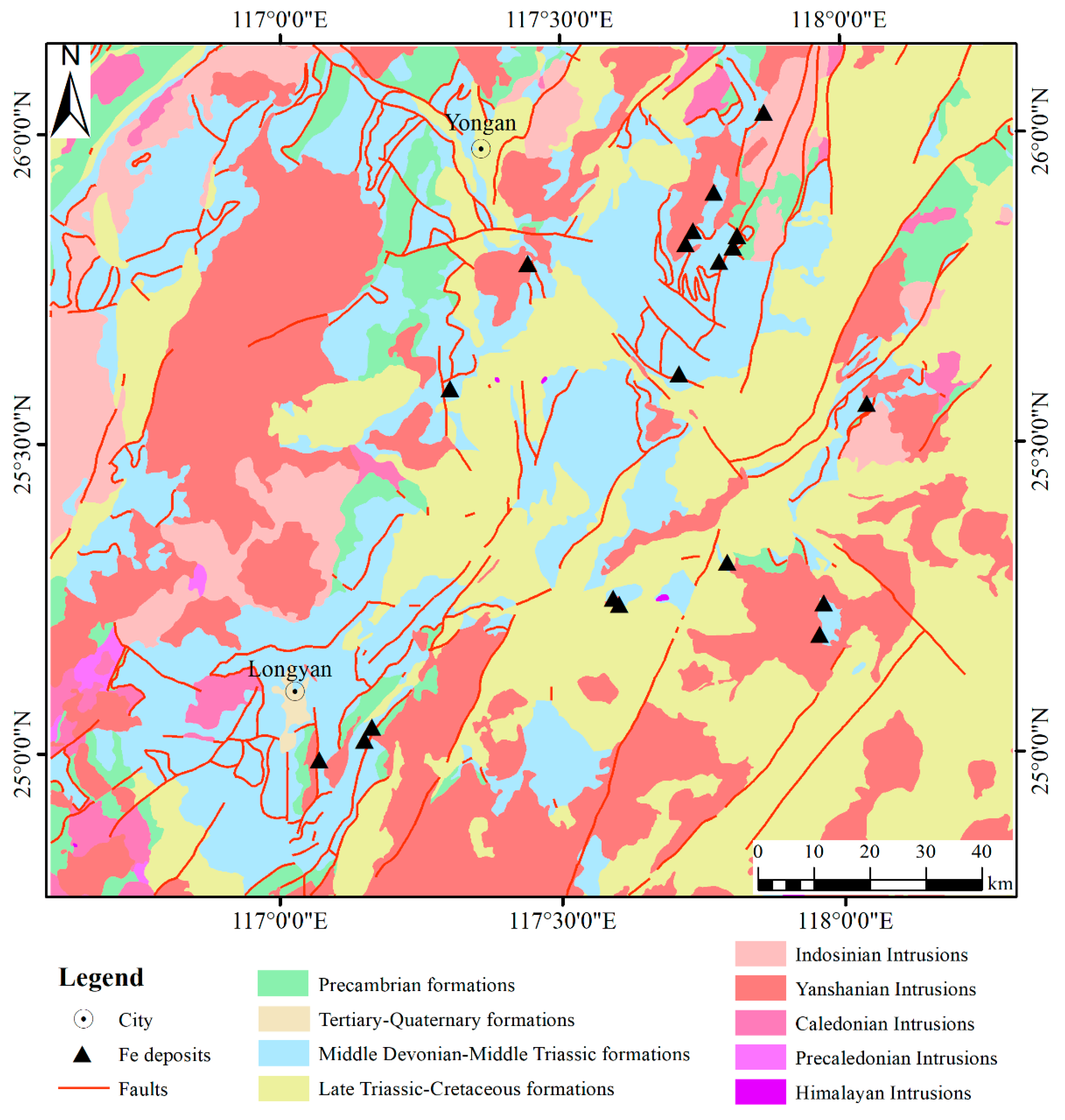
The study area (Figure 2) is located in the southwestern Fujian metallogenic belt (SFMB), and has been extensively studied in terms of geology and tectonic evolution [74,75,76]. The skarn-type Fe-polymetallic mineralization occurred in the SFMB is related to the Mesozoic tectonic magmatism and the late Paleozoic interbedded clastic and carbonate sedimentary rocks [75]. The NE-NNE-trending faults, well developed in the SFMB, provide pathways for the ore-forming fluid. Studies have indicated that the association of geochemical elements related to Fe-polymetallic mineralization includes Fe, Pb, Zn, Cu, Au, Ag, Sb, Sn, Mo, W [75]. The SFMB is located in the subtropical monsoon climate zone, blessed with plentiful rain and a mild climate. Such climate characteristics benefit the extensive development of vegetation [77]. The landscape in this area mainly consists of low, rolling hills. Chemical weathering is relatively dominant under such conditions, and a large amount of organic matter and clay minerals can be found in the soil profile [78]. The extensively developed streams can cause significant dispersion of geochemical elements [79]. Such a wide range of secondary geological processes involved in the landscape evolution might lead to strong variation of geochemical elements and modify their associations.
3.2. Geochemical Data
The geochemical dataset used in current study was collected as part of the Regional Geochemistry-National Reconnaissance (RGNR) project in China, initiated in January 1979. The dataset consisted of 6380 stream sediment samples. The sampling density was one composite sample per 4 km2. A total of 39 elements were determined for each sample. The analytical schemes for determining the concentrations of these elements included X-ray fluorescence (Al, Fe, K, P, Si, Cr, Ti, Y and Zr), inductively coupled plasma mass spectrometry (Cu, Pb, Bi, Cd, Co, Mo, W, La, Nb, Th and U), inductively coupled plasma atomic emission spectrometry (Ba, Be, Li, Ca, Mg, Na, Sr, Ni, Mn, V and Zn), emission spectrometry (Ag, B and Sn), hydride generation atomic fluorescence spectrometry (As and Sb), ion selective electrode (F), cold vapor atomic fluorescence spectrometry (Hg) and graphite furnace atomic absorption spectrometry (Au). The details about the sampling, analysis, quality control and detection limit of the geochemical data can be found in [80,81]. The mineralization-associated trace elements Pb, Zn, Cu, Au, Ag, Sb, Sn, Mo, W, were selected and analyzed here to explore their complex distribution patterns and associations.
4. Results and Discussions
4.1. Frequency Distribution Characteristics
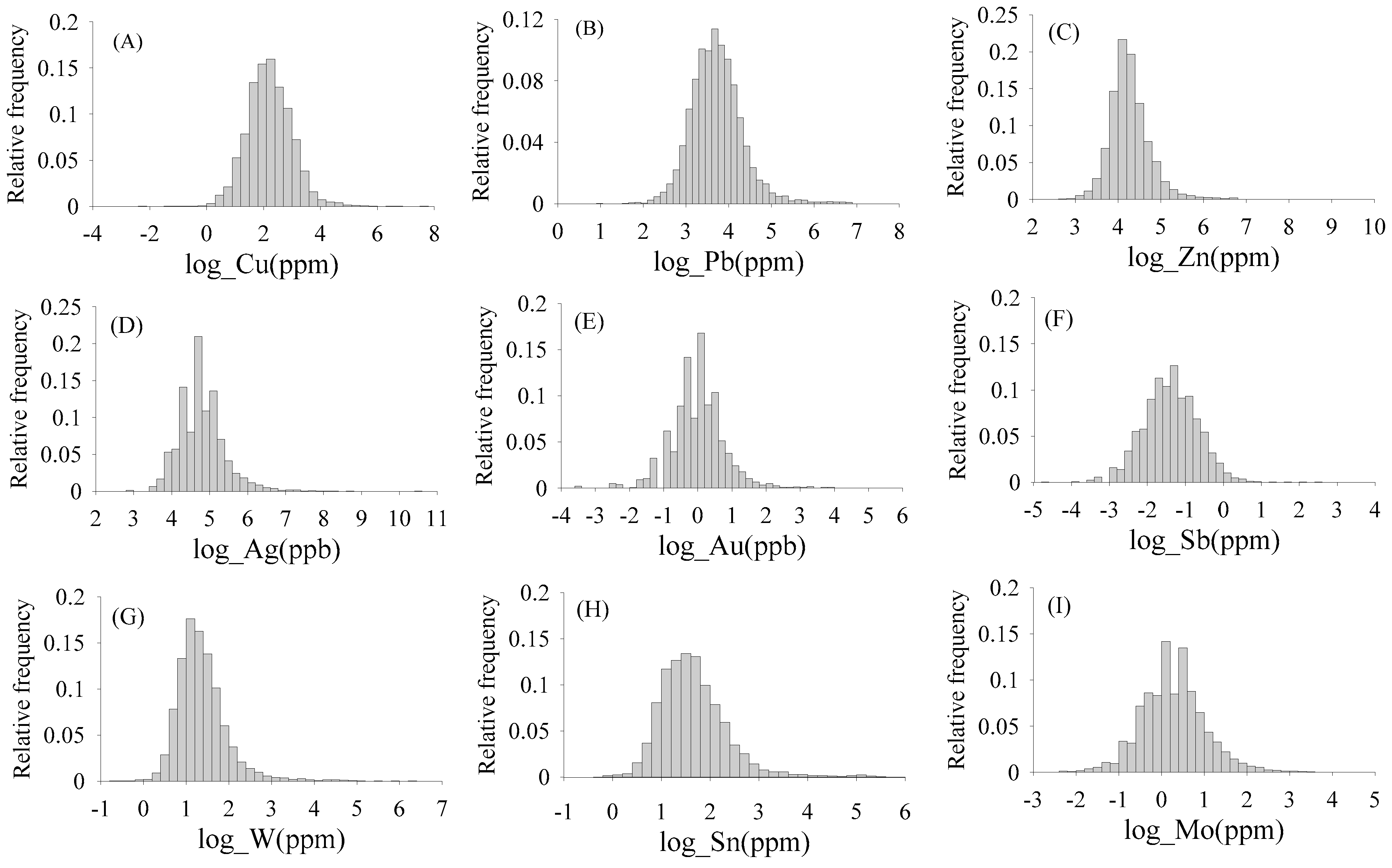
The frequency distributions of trace elements are heavily positively skewed, as indicated by the skewness in Table 1. The histograms of the log-transformed data (Figure 3) indicate that approximately lognormal distribution patterns can be observed for Cu and Pb. The histograms of log-transformed Zn, W and Sn are analogous and slightly positively-skewed. The elements of Ag and Au show similar and relatively strong variation patterns. The statistics (Table 1) also suggest that W, Au, and Ag have greater CVs than other elements. The elements of Cu, Ag and Zn simultaneously have large values for CV, skewness and kurtosis. The element of Au has evidently the largest CV, but its skewness and kurtosis are not that predominant with respect to Ag and Cu. Such observations indicate that these mineralization-related elements might be subject to different geological processes, which might impose great effect on the distribution patterns of elements and their associations.
4.2. Spatial Distribution Characteristics
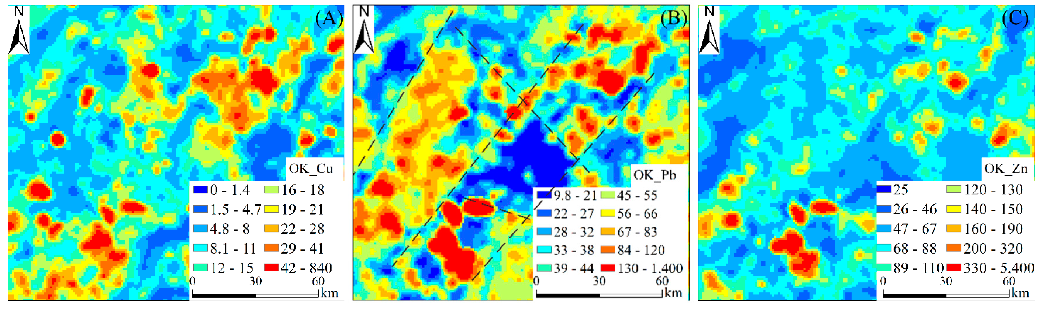
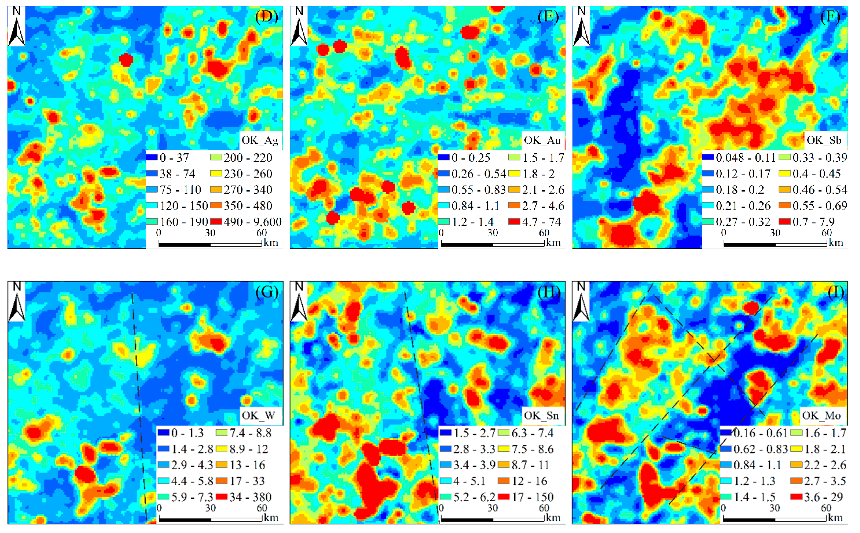
The spatial distributions of the selected trace elements were created by interpolating the stream sediment data using ordinary kriging (OK). The grid size was chosen to be 1 km × 1 km. All the interpolated maps are displayed by classifying the values into 10 groups using quantiles in ArcGIS (Version 10.4, Environmental Systems Research Institute, Redlands, CA, USA), each equally occupying 10 percent of the variation range (Figure 4). An observation is that the distributions of Cu, Mo, Pb, and Zn clearly extend along the NE direction, implying the likely control of the regional tectonic activities in the study area. The distributions of Au, Ag, W and Sn vary more strongly, and spatial anisotropy is not that evident with respect to other elements. Additionally, the nugget effect can be easily observed for the spatial distributions of Au and Ag. The negatively correlated relationship between W, Mo, Pb and Sb can also be identified.
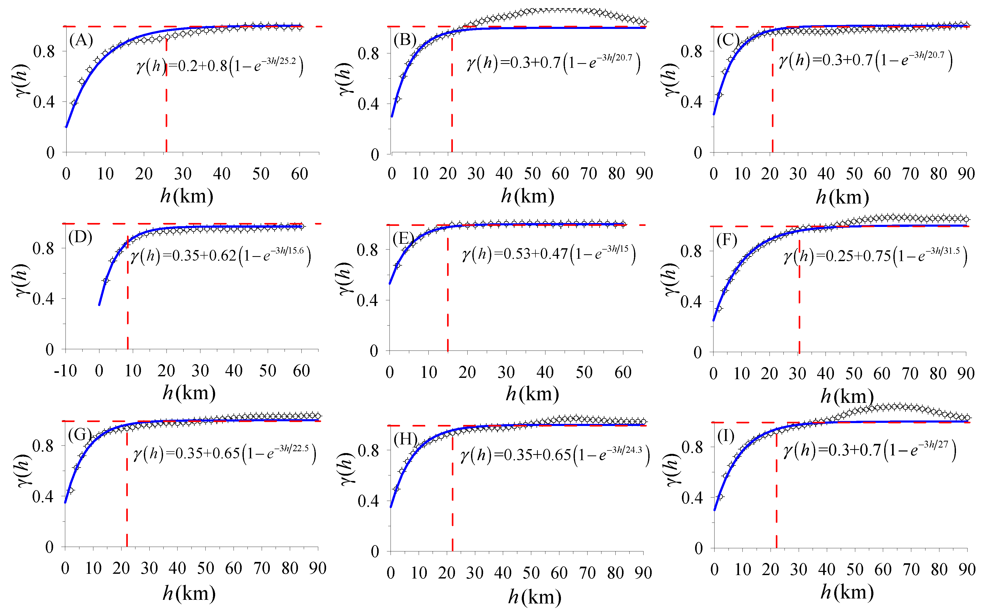
The semivariograms and the fitted exponential variogram model suggest the spatial autocorrelation of the selected geochemical elements (Figure 5). The elements of Au and Ag show a relatively weak spatial correlation (range < 20 km), Cu, Pb, Zn, W, Sn and Mo show moderate spatial correlation (20 km < range < 30 km), while Sb exhibits a relatively strong spatial correlation (range > 30 km). The NSRs were derived from the fitted variogram models to reflect the degree of local variation (Table 1). The nugget effect for Au is significant, and the usual interpretation for this phenomenon is that the gold minerals are usually associated with the presence of nuggets of gold [82]. In addition, the local continuity of Ag, W and Sn is relatively weak as well. Another observation is that Pb and Zn have the same range and NSR, although their spatial distributions seem to be a little different especially in the northwestern part (Figure 4). Exponential variogram models can fit the experimental semivariograms well for Cu, Zn, Ag and Au, in that the semivariograms closely reach the expected sill variance without evident deviation. However, the semivariograms for Pb, Sb, W, Sn and Mo exceed the theoretical sill of 1. Such an observation is usually due to the presence of a large-scale trend within the geochemical distributions [83]. A subtle trend can be observed from the spatial distributions of W and Sn, that is, the concentrations in the left half part are relatively higher than those in the right part (Figure 4). The semivariograms for several elements (e.g., Pb and Mo) keep increasing beyond the expected sill, and then decrease, starting from ~60 km. One possible interpretation for this is the “hole effect”, where cyclic variation patterns in geologic quantities can impart a fluctuation behavior to the semivariogram. In this study, several boundaries can be easily identified in the spatial distributions of these elements, and those for Pb and Mo are showed here (Figure 4). These boundaries define cyclic variation patterns that might be related to the observed behavior in semivariograms.
The multifractal spectra of the elements were derived by the moment method [63]. The values of α0, ∆α and R, as displayed in Table 1, were cited from Zuo [30]. The multifractal spectra of the elements exhibit different patterns. All the trace elements possess multifractal properties, with ∆α being greater than 0. The multifractal spectra for all the trace elements but Cu deviate to the left (R > 1), indicating the enrichment patterns are predominant in their spatial distributions. Zhang [84] indicated that Cu is slightly depleted in the stream sediment in SFMB, which agrees with the result of multifractal analysis here. The asymmetry indexes R for the major ore-forming elements Ag, W, Sn, Mo and Zn are relatively larger than for other elements, suggesting local geological processes might be superimposed and greatly contribute to the accumulation of these elements.
To investigate the stratified heterogeneity for the mineralization-related elements, five groups were defined based on the geological settings: (1) Precambrian formations, (2) middle Devonian-middle Triassic formations, (3) late Triassic-Cretaceous formations, (4) Yanshanian intrusions, and (5) intrusions of other geological ages (Figure 2). The regions covered by Tertiary and Quaternary formations were not allowed for, due to the very limited amount of samples falling into them (< 5). The q-statistics for the trace elements show that Cu, Mo and Sb exhibit relatively strong spatial heterogeneity, suggesting that the controls of the lithology across the study area on the distribution of the elements are relatively important. The stratified heterogeneity for Zn, Au and Ag is weak, indicating that their distribution patterns are not closely associated with geological lithology due to secondary dispersion or other processes.
4.3. Exploring the Association of Geochemical Elements
The characteristics of trace elements in terms of frequency distribution, spatial autocorrelation and self-similarity are complex, in that different associations can be identified when considering different distribution properties. It can be summarized that Ag shows strong variation whichever property is allowed for; the spatial variation patterns of Pb and Zn are similar, but their frequency distribution parameters are significantly different; the distribution properties of Cu show large similarity with Zn, except for the asymmetry of multifractal spectra and heterogeneity.
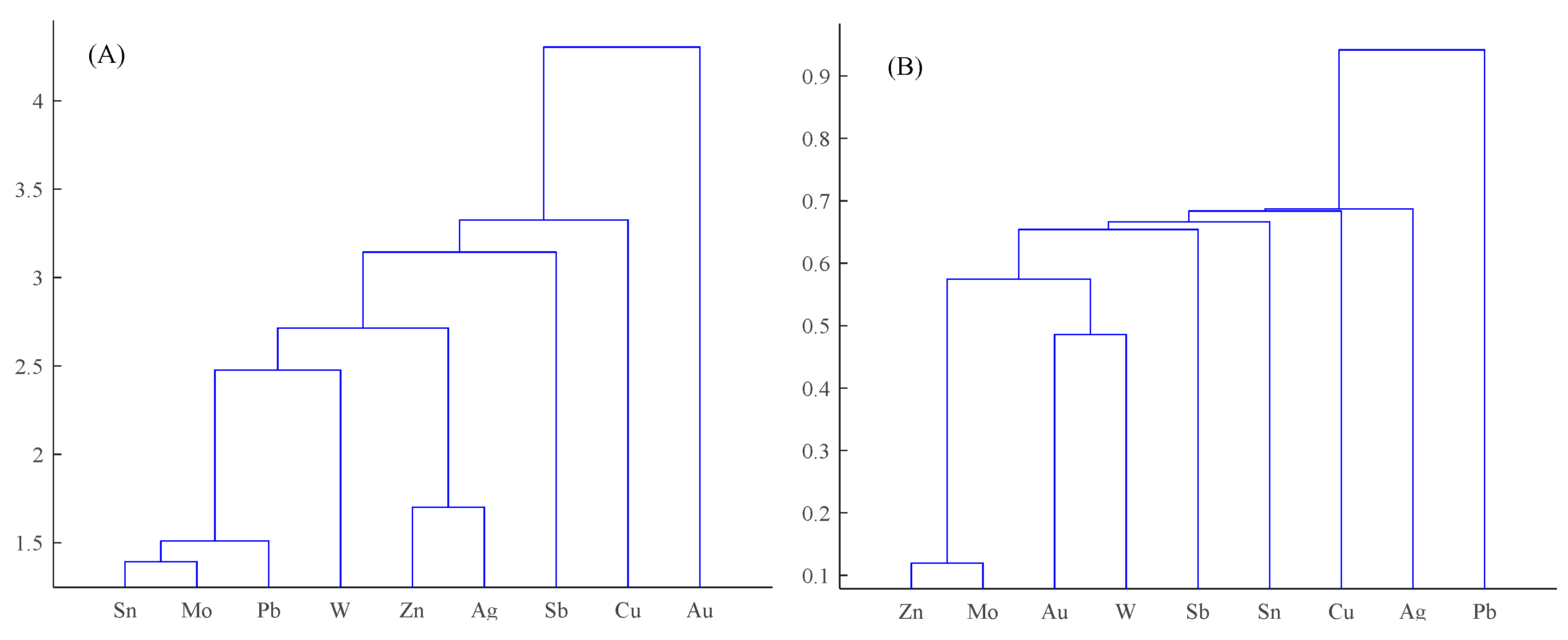
The association of geochemical elements are explored in this section by clustering the elements based on the parameters of both frequency and spatial distributions (Table 1). The data for each property were normalized into [0, 1] prior to hierarchical clustering. The clustering result (Figure 6A) shows that Mo and Sn are firstly clustered, with Pb and W in turn being grouped into this group. The elements of Ag and Zn are also relatively more relevant, both being characterized by large skewness and kurtosis, and their spatial distribution properties are also comparative. The elements of Au, Cu and Sb exhibit distinctive characteristics, such that they did not show clear association with other elements. The result from conventional clustering analysis is also presented for comparison (Figure 6B). The element associations are significantly different, in that Zn and Mo are closely clustered, Au and W are moderately associated, and the characteristics of Pb seem to be distinctive from other elements. Such a large deviation can be expected due to the fact that the conventional clustering analysis fails to consider spatial distribution characteristics.
The IV values in Equation (8) were calculated subsequently to get the importance ranking of properties in clustering the elements. Two cases were tested: the first one considers four groups ({Pb, Zn, Ag, W, Sn, Mo}, {Cu}, {Au}, {Sb}) and the second considers five groups ({Zn, Ag}, {Pb, W, Sn, Mo}, {Cu}, {Au}, {Sb}). For the first case, the importance ranking obtained is IV(q) = 7.14 > IV(nugget/sill) = 7.10 > IV(Δα) = 6.14 > IV(α0) = 3.49 > IV(range) = 2.62 > IV(CV) = 0.16 > IV(R) = −3.28 > IV(skewness) = -7.23. For the second case, the importance ranking is IV(R) = 7.52 > IV(q) = 7.45 > IV(nugget/sill) = 7.1 > IV(Δα) = 6.94 > IV(skewness) = 6.51 > IV(range) = 5.5 > IV(α0) = 4.8 > IV(CV) = 0.89. It can be seen that the frequency distribution parameters play a less important role than the spatial properties in clustering the geochemical elements for both the two cases. The elements in the association of {Pb, Sn, Mo} have very similar spatial heterogeneity, which might dominate their association. The spatial autocorrelation and scaling property also impose important effects on the association of {Pb, Sn, Mo}. The spatial distributions of Pb, Sn and Mo (Figure 4) show that they are controlled by the Yanshanian intrusions. Zhang [84] confirmed that Pb and Mo shows good correlation with tin mineralization and served as a critical geochemical signature for the discovery of Sn-polymetallic deposits in the study area. Lin [75] indicated that Sn, Pb, Mo, W and Zn are important ore-forming elements associated with Yanshanian granites, and they show close spatial and genetic relations with each other. In addition, Pb, Mo and Sn can be present as immobile or heavy minerals in the surficial environment, which might also contribute to the association observed [28]. However, the clustering structure for other elements is not that clear as {Pb, Sn, Mo}, suggesting that the varying patterns of these trace elements are complex resulting from diagenesis and secondary dispersions. The importance ranking analysis shows that geological lithology is still the dominant factor for element distributions and their associations. More detailed analyses of the mineralogy and landscape geochemistry need to be performed to investigate the elemental behaviors.
5. Conclusions
The distribution of geochemical elements in the surficial environment exhibits complex patterns due to the diverse geological processes involved. This study explored the distribution characteristics of geochemical elements and their associations from the aspects of frequency distribution, spatial autocorrelation, spatial heterogeneity and self-similarity. The following conclusions can be drawn:
(1) Studies of the frequency and spatial distribution characteristics of trace elements can enhance the knowledge of elemental behaviors and hence their association. The presented workflow of clustering the geochemical elements based on the parameters of frequency and spatial distributions provides an alternative way to identify the association of geochemical elements. The association identified by the method presented can be different from that determined by correlation coefficient-based cluster analysis.
(2) The case study presented here illustrates and validates the workflow for exploring the distribution characteristics of geochemical elements and their associations. Spatial heterogeneity, autocorrelation and self-similarity are important characteristics in grouping elements in this study. It indicates that the spatial distribution characteristics should not be neglected when identifying element associations. The findings can improve our knowledge of the geology and geochemistry in the study area and might benefit further mineral exploration.
Author Contributions
Conceptualization, R.Z.; methodology, J.W. and R.Z.; formal analysis, J.W.; investigation, R.Z. and J.W.; resources, R.Z.; writing–original draft preparation, J.W.; writing–review and editing, R.Z.; visualization, J.W.; funding acquisition, R.Z. and J.W. All authors have read and agreed to the published version of the manuscript.
Funding
This research benefited from the joint financial support from the Scientific Research Foundation for the Youth Teachers of Chengdu University of Technology (10912-KYQD-07280), the Foundation for Backbone of Teachers of Chengdu University of Technology (10912-2019KY01-07280), and National Natural Science Foundation of China (No. 41772344).
Acknowledgments
Thanks are due to the editor and two anonymous reviewers for their comments and suggestions, which helped improve this study.
Conflicts of Interest
The authors declare no conflict of interest.
References
- Cheng, Q. Multiplicative cascade processes and information integration for predictive mapping. Nonlinear Process. Geophys. 2012, 19, 57–68. [Google Scholar] [CrossRef] [Green Version]
- Xie, S.; Bao, Z. Fractal and Multifractal Properties of Geochemical Fields. Math. Geol. 2004, 36, 847–864. [Google Scholar] [CrossRef]
- De Caritat, P.; Grunsky, E.C. Defining element associations and inferring geological processes from total element concentrations in Australian catchment outlet sediments: Multivariate analysis of continental-scale geochemical data. Appl. Geochem. 2013, 33, 104–126. [Google Scholar] [CrossRef]
- Coker, W.B. Future research directions in exploration geochemistry. Geochem. Explor. Environ. Anal. 2010, 10, 75–80. [Google Scholar] [CrossRef]
- Grunsky, E.C. The interpretation of geochemical survey data. Geochem. Explor. Environ. Anal. 2010, 10, 27–74. [Google Scholar] [CrossRef]
- Bölviken, B.; Stokke, P.R.; Feder, J.; Jössang, T. The fractal nature of geochemical landscapes. J. Geochem. Explor. 1992, 43, 91–109. [Google Scholar] [CrossRef]
- Cheng, Q.; Agterberg, F.P.; Ballantyne, S.B. The separation of geochemical anomalies from background by fractal methods. J. Geochem. Explor. 1994, 51, 109–130. [Google Scholar] [CrossRef]
- Allegre, C.J.; Lewin, E. Scaling laws and geochemical distributions. Earth Planet. Sci. Lett. 1995, 132, 1–13. [Google Scholar] [CrossRef]
- Agterberg, F.P. New applications of the model of de Wijs in regional geochemistry. Math. Geosci. 2007, 39, 1–26. [Google Scholar] [CrossRef]
- Chen, G.; Cheng, Q. Fractal-based wavelet filter for separating geophysical or geochemical anomalies from background. Math. Geosci. 2018, 50, 249–272. [Google Scholar] [CrossRef]
- Ge, Y.; Jin, Y.; Stein, A.; Chen, Y.; Wang, J.; Wang, J.; Cheng, Q.; Bai, H.; Liu, M.; Atkinson, P.M. Principles and methods of scaling geospatial Earth science data. Earth-Sci. Rev. 2019, 102897. [Google Scholar] [CrossRef]
- Goodchild, M.F. Scale in GIS: An overview. Geomorphology 2011, 130, 5–9. [Google Scholar] [CrossRef]
- Tobler, W.R. A computer movie simulating urban growth in the Detroit region. Econ. Geogr. 1970, 46 (Suppl. 1), 234–240. [Google Scholar] [CrossRef]
- Matheron, G. Traite de Geostatistique Appliquee; Editions Technip: Mémoires, France, 1962. [Google Scholar]
- Cressie, N. Statistics for Spatial Data; John Wiley & Sons, Inc.: New York, NY, USA, 1993. [Google Scholar]
- Goovaerts, P. Geostatistics for Natural Resources Evaluation; Oxford University Press: New York, NY, USA, 1997. [Google Scholar]
- Chilès, J.P.; Delfiner, P. Geostatistics: Modeling Spatial Uncertainty; Wiley: Hoboken, NJ, USA, 2012. [Google Scholar]
- Wang, J.; Zuo, R. An extended local neighborhood gap statistic for identifying geochemical anomalies. J. Geochem. Explor. 2016, 164, 86–93. [Google Scholar] [CrossRef]
- Zuo, R. Identification of geochemical anomalies associated with mineralization in the Fanshan district, Fujian, China. J. Geochem. Explor. 2014, 139, 170–176. [Google Scholar] [CrossRef]
- Xiong, Y.; Zuo, R.; Wang, K.; Wang, J. Identification of geochemical anomalies via local RX anomaly detector. J. Geochem. Explor. 2018, 189, 64–71. [Google Scholar] [CrossRef]
- Mandelbrot, B.B. The Fractal Geometry of Nature; WH Freeman: New York, NY, USA, 1983; p. 497. [Google Scholar]
- Cheng, Q. Multifractality and spatial statistics. Comput. Geosci. 1999, 25, 949–961. [Google Scholar] [CrossRef]
- Cheng, Q. Mapping singularities with stream sediment geochemical data for prediction of undiscovered mineral deposits in Gejiu, Yunnan Province, China. Ore Geol. Rev. 2007, 32, 314–324. [Google Scholar] [CrossRef]
- Baranowski, P.; Krzyszczak, J.; Slawinski, C.; Hoffmann, H.; Kozyra, J.; Nieróbca, A.; Siwek, K.; Gluza, A. Multifractal analysis of meteorological time series to assess climate impacts. Clim. Res. 2015, 65, 39–52. [Google Scholar] [CrossRef] [Green Version]
- Dutta, S. Decoding the Morphological Differences between Himalayan Glacial and Fluvial Landscapes Using Multifractal Analysis. Sci. Rep. 2017, 7, 11032. [Google Scholar] [CrossRef] [Green Version]
- Rodríguez-Lado, L.; Lado, M. Relation between soil forming factors and scaling properties of particle size distributions derived from multifractal analysis in topsoils from Galicia (NW Spain). Geoderma 2017, 287, 147–156. [Google Scholar] [CrossRef]
- Hawkes, H.E.; Webb, J.S. Geochemistry in Mineral Exploration; Harper & Row, Pulishers: New York, NY, USA; Evanston, IL, USA, 1962. [Google Scholar]
- Siegel, F.R. Applied Geochemistry; Wiley: New York, NY, USA, 1974. [Google Scholar]
- Beus, A.A.; Grigorian, S.V. Geochemical Exploration Methods for Mineral Deposits; Applied Publishing Ltd.: Wilmette, IL, USA, 1977; p. 287. [Google Scholar]
- Zuo, R. Selection of an elemental association related to mineralization using spatial analysis. J. Geochem. Explor. 2018, 184, 150–157. [Google Scholar] [CrossRef]
- Nicholson, K. Contrasting mineralogical geochemical signatures of manganese oxides guides to metallogenesis. Econ. Geol. 1992, 87, 1253–1264. [Google Scholar] [CrossRef]
- Pons, J. Geology, petrography and geochemistry of igneous rocks related to mineralized skarns in the NW Neuquén basin, Argentina: Implications for Cordilleran skarn exploration. Ore Geol. Rev. 2010, 38, 37–58. [Google Scholar] [CrossRef]
- Cárdenes, V.; Rubio-Ordoñez, A.; Monterroso, C.; Calleja, L. Geology and geochemistry of Iberian roofing slates. Chem. Der Erde-Geochem. 2013, 73, 373–382. [Google Scholar]
- Tong, Y.; Gong, Q.; Han, D.; Liu, N.; Xu, Z.; Yu, W. Indicator Element Association in Geochemical Surveys: A Case Study of the Niutougou Gold Deposit in Western Henan Province. Geol. Explor. 2014, 50, 712–724, (In Chinese with English abstract). [Google Scholar]
- Valkama, M.; Sundblad, K.; Nygard, R.; Cook, N. Mineralogy and geochemistry of indium-bearing polymetallic veins in the Sarvlaxviken area, Lovisa, Finland. Ore Geol. Rev. 2016, 75, 206–219. [Google Scholar] [CrossRef]
- Costa, M.L.; Angélica, R.S.; Costa, N.C. The geochemical association Au-As-B-(Cu)-Sn-W in latosol, colluvium, lateritic iron crust and gossan in Carajas, Brazil: Importance for primary ore identification. J. Geochem. Explor. 1999, 67, 33–49. [Google Scholar] [CrossRef]
- Cluer, J.K. Remobilized geochemical anomalies related to deep gold zones, carlin trend, Nevada. Econ. Geol. 2012, 107, 1343–1349. [Google Scholar] [CrossRef]
- Forbes, C.; Giles, D.; Freeman, H.; Sawyer, M.; Normington, V. Glacial dispersion of hydrothermal monazite in the Prominent Hill deposit: An exploration tool. J. Geochem. Explor. 2015, 156, 10–33. [Google Scholar] [CrossRef]
- Li, H.; Zhang, W.; Liu, B.; Wang, J.; Guo, R. The study on axial zonality sequence of primary halo and some criteria for the application of this sequence for major types of gold deposits in china. Geol. Prospect. 1999, 35, 32–35. [Google Scholar]
- Harraz, H.Z.; Hamdy, M.M. Zonation of primary haloes of Atud auriferous quartz vein deposit, Central Eastern Desert of Egypt: A potential exploration model targeting for hidden mesothermal gold deposits. J. Afr. Earth Sci. 2015, 101, 1–18. [Google Scholar] [CrossRef]
- Robb, L. Introduction to Ore-Forming Processes; Blackwell Publishing: Malden, MA, USA, 2004. [Google Scholar]
- Nichol, I.; Garrett, R.G.; Webb, J.S. The role of some statistical and mathematical methods in the interpretation of regional geochemical data. Econ. Geol. 1969, 64, 204–220. [Google Scholar] [CrossRef]
- Garrett, R.G. The chi-square plot: A tool for multivariate outlier recognition. J. Geochem. Explor. 1989, 32, 319–341. [Google Scholar] [CrossRef]
- Davis, J.C. Statistics and Data Analysis in Geology, 3rd ed.; John Wiley and Sons: New York, NY, USA, 2002; p. 656. [Google Scholar]
- Carranza, E.J.M. Geochemical Anomaly and Mineral Prospectivity Mapping in GIS. Handb. Explor. Environ. Geochem. 2009, 11, 85–113. [Google Scholar]
- Reimann, C.; Filzmoser, P.; Garrett, R.; Dutter, R. Statistical Data Analysis Explained: Applied Environmental Statistics with R; John Wiley & Sons: Chichester, UK, 2011; p. 362. [Google Scholar]
- Pawlowsky-Glahn, V.; Egozcue, J.J.; Tolosana-Delgado, R. Modeling and Analysis of Compositional Data; John Wiley & Sons: Chichester, UK, 2015. [Google Scholar]
- Parsa, M.; Maghsoudi, A.; Yousefi, M.; Sadeghi, M. Recognition of significant multi-element geochemical signatures of porphyry Cu deposits in Noghdouz area, NW Iran. J. Geochem. Explor. 2016, 165, 111–124. [Google Scholar] [CrossRef]
- Grunsky, E.C.; de Caritat, P. State-of-the-art analysis of geochemical data for mineral exploration. Geochem. Explor. Environ. Anal. 2019. [Google Scholar] [CrossRef]
- Ali, K.; Cheng, Q.; Li, W.; Chen, Y. Multielement association analysis of stream sediment geochemistry data for predicting gold deposits in southcentral Yunnan Province, China. Geochem. Explor. Environ. Anal. 2006, 6, 341–348. [Google Scholar] [CrossRef]
- Zhang, W.; Chen, L.; Zhang, G.; Xin, Z.; Hu, X. Compilation of geochemical integrated-anomaly map in Chongjiang area of Tibet. Comput. Tech. Geophys. Geochem. Explor. 2010, 32, 651–655, (In Chinese with English Abstract). [Google Scholar]
- Liu, B.; Guo, K.; Ao, D.; Wu, J. Application and exploration of JADE in searching the combination of geochemical ore-forming elements. Comput. Tech. Geophys. Geochem. Explor. 2012, 34, 58–61, (In Chinese with English Abstract). [Google Scholar]
- Yousefi, M.; Kamkar-Rouhani, A.; Carranza, E.J.M. Geochemical mineralization probability index (GMPI): A new approach to generate enhanced stream sediment geochemical evidential map for increasing probability of success in mineral potential mapping. J. Geochem. Explor. 2012, 115, 24–35. [Google Scholar] [CrossRef]
- Yousefi, M.; Kamkar-Rouhani, A.; Carranza, E.J.M. Application of staged factor analysis and logistic function to create a fuzzy stream sediment geochemical evidence layer for mineral prospectivity mapping. Geochem. Explor. Environ. Anal. 2014, 14, 45–58. [Google Scholar] [CrossRef]
- Lee, C.W.; Tsai, W.H. Compositional data analysis of hydrothermal alteration in IOCG systems, Great Bear magmatic zone, Canada: To each alteration type its own geochemical signature. Geochem. Explor. Environ. Anal. 2013, 13, 229–247. [Google Scholar]
- Harraz, H.Z.; Hamdy, M.M.; El-Mamoney, M.H. Multielement association analysis of stream sediment geochemistry data for predicting gold deposits in Barramiya gold mine, Eastern Desert, Egypt. J. Afr. Earth Sci. 2012, 68, 1–14. [Google Scholar] [CrossRef]
- Zhao, J.; Chen, S.; Zuo, R. Identifying geochemical anomalies associated with Au–Cu mineralization using multifractal and artificial neural network models in the Ningqiang district, Shaanxi, China. J. Geochem. Explor. 2016, 164, 54–64. [Google Scholar] [CrossRef]
- Zhao, J.; Wang, W.; Cheng, Q. Application of geographically weighted regression to identify spatially non-stationary relationships between Fe mineralization and its controlling factors in eastern Tianshan, China. Ore Geol. Rev. 2014, 57, 628–638. [Google Scholar] [CrossRef]
- Zhao, J.; Zuo, R.; Chen, S.; Kreuzer, O.P. Application of the tectono-geochemistry method to mineral prospectivity mapping: A case study of the Gaosong tin-polymetallic deposit, Gejiu district, SW China. Ore Geol. Rev. 2015, 71, 719–734. [Google Scholar] [CrossRef]
- Cambardella, C.A.; Moorman, T.B.; Parkin, T.B.; Karlen, D.L.; Novak, J.M.; Turco, R.F.; Konopka, A.E. Field-scale variability of soil properties in central Iowa soils. Soil Sci. Soc. Am. J. 1994, 58, 1501–1511. [Google Scholar] [CrossRef]
- Evertsz, C.J.G.; Mandelbrot, B.B. Multil’ractal measures. In Chaos and Fractals; Peitgen, H.O., Jurgens., H., Saupe, D., Eds.; Springer: New York, NY, USA, 1992; pp. 922–953. [Google Scholar]
- Feder, J. Fractals; Plenum Press: New York, NY, USA, 1988; p. 283. [Google Scholar]
- Halsey, T.C.; Jensen, M.H.; Kadanoff, L.P.; Procaccia, I.; Shraiman, B.I. Fractal measures and their singularities: The characterization of strange sets. Phys. Rev. A 1986, 2, 501–511. [Google Scholar] [CrossRef]
- Schertzer, D.; Lovejoy, S. Nonlinear Variability in Geophysics; Kluwer Academic Publishers: Dordrecht, The Netherlands, 1991; p. 318. [Google Scholar]
- Agterberg, F.P. Fractals, multifractals and change of support. In Geostatistics for the Next Century; Dimitrakopoulos, P., Ed.; Kluwer Academic Publishers: Dordrecht, The Netherlands, 1994; pp. 223–234. [Google Scholar]
- Cheng, Q. Generalized binomial multiplicative cascade processes and asymmetrical multifractal distributions. Nonlinear Process. Geophys. 2014, 21, 477–487. [Google Scholar] [CrossRef] [Green Version]
- Zuo, R.; Cheng, Q.; Agterberg, F.P.; Xia, Q. Application of singularity mapping technique to identify local anomalies using stream sediment geochemical data, a case study from Gangdese, Tibet, western China. J. Geochem. Explor. 2009, 101, 225–235. [Google Scholar] [CrossRef]
- Gonçalves, M.A. Characterization of Geochemical Distributions Using Multifractal Models. Math. Geol. 2001, 33, 41–61. [Google Scholar] [CrossRef]
- Schertzer, D.; Lovejoy, S. Physical modeling and analysis of rain and clouds by anisotropic scaling multiplicative processes. J. Geophys. Res. Atmos. 1987, 92, 9693–9714. [Google Scholar] [CrossRef]
- Cheng, Q.; Agterberg, F.P. Multifractal modeling and spatial statistics. Math. Geol. 1996, 28, 1–16. [Google Scholar] [CrossRef]
- Wang, J.F.; Zhang, T.L.; Fu, B.J. A measure of spatial stratified heterogeneity. Ecol. Indic. 2016, 67, 250–256. [Google Scholar] [CrossRef]
- Johnson, S.C. Hierarchical clustering schemes. Psychometrika 1967, 32, 241–254. [Google Scholar] [CrossRef]
- Rokach, L.; Maimon, O. Clustering methods. In Data Mining and Knowledge Discovery Handbook; Springer: Boston, MA, USA, 2005; pp. 321–352. [Google Scholar]
- Mao, J.; Xu, N.; Hu, Q.; Xing, G.; Yang, Z. The Mesozoic rock-forming and oreforming processes and tectonic environment evolution in Shanghang–Datian region, Fujian. Acta Petrol. Sin. 2004, 20, 285–296, (In Chinese with English Abstract). [Google Scholar]
- Lin, D. Research on Late Paleozoic-Triassic Tectonic Evolution and Metallogenetic Regularities of Iron-Polymetalic Deposits in the Southwestern Fujian Province. Ph.D. Thesis, China University of Geosciences, Beijing, China, 2011. [Google Scholar]
- Zhong, J.; Chen, Y.J.; Chen, J.; Qi, J.P.; Dai, M.C. Geology and fluid inclusion geochemistry of the Zijinshan high-sulfidation epithermal Cu-Au deposit, Fujian Province, SE China: Implication for deep exploration targeting. J. Geochem. Explor. 2018, 184, 49–65. [Google Scholar] [CrossRef]
- Xiang, Y.; Mou, X.; Ren, T. Geochemical Prospecting Materials for Potential Assessment of Mineral Resources in China and Applications; Geological Publishing House: Beijing, China, 2018; p. 445. [Google Scholar]
- Butt, C.R.M. The development of regolith exploration geochemistry in the tropics and sub-tropics. Ore Geol. Rev. 2016, 73, 380–393. [Google Scholar] [CrossRef]
- Zhang, X. Study on Spatial Acidification Variation in Cropland Soil and Its Driving Factors. Ph.D. Thesis, Fujian Agriculture and Forestry University, Fuzhou, China, 2017. [Google Scholar]
- Wang, X.; Xie, X.; Zhang, B.; Hou, Q. Geochemical probe into China’s continental crust. Acta Geosci. Sin. 2011, 32, 65–83, (In Chinese with English Abstract). [Google Scholar]
- Xie, X.; Mu, X.; Ren, T. Geochemical mapping in China. J. Geochem. Explor. 1997, 60, 99–113. [Google Scholar]
- Journel, A.G.; Huijbregts, C.J. Mining Geostatistics; Academic Press: London, UK, 1978; Volume 600. [Google Scholar]
- Gringarten, E.; Deutsch, C.V. Teacher’s aide variogram interpretation and modeling. Math. Geol. 2001, 33, 507–534. [Google Scholar] [CrossRef]
- Zhang, D. Tectonic Evolution and Tin Polymetal Regional Metallogenesis in Southwestern Fujian Province. Ph.D. Thesis, Chinese Academy of Geological Sciences, Beijing, China, 1999. [Google Scholar]
Figure 1.
The workflow to explore distribution characteristics and association of geochemical elements.
Figure 1.
The workflow to explore distribution characteristics and association of geochemical elements.

Figure 2.
Simplified geological map of the southwestern Fujian metallogenic belt (modified from Zuo [30]).
Figure 2.
Simplified geological map of the southwestern Fujian metallogenic belt (modified from Zuo [30]).

Figure 3.
Histograms of 9 selected geochemical elements after logarithmic transformation. (A) Cu, (B) Pb, (C) Zn, (D) Ag, (E) Au, (F) Sb, (G) W, (H) Sn, (I) Mo. Note that the frequency in y-axis have been normalized by the sample size.
Figure 3.
Histograms of 9 selected geochemical elements after logarithmic transformation. (A) Cu, (B) Pb, (C) Zn, (D) Ag, (E) Au, (F) Sb, (G) W, (H) Sn, (I) Mo. Note that the frequency in y-axis have been normalized by the sample size.

Figure 4.
Maps showing the spatial distributions of interpolated geochemical elements using OK. (A) Cu, (B) Pb, (C) Zn, (D) Ag, (E) Au, (F) Sb, (G) W, (H) Sn, (I) Mo.
Figure 4.
Maps showing the spatial distributions of interpolated geochemical elements using OK. (A) Cu, (B) Pb, (C) Zn, (D) Ag, (E) Au, (F) Sb, (G) W, (H) Sn, (I) Mo.


Figure 5.
Semivariograms of 9 selected geochemical elements. (A) Cu, (B) Pb, (C) Zn, (D) Ag, (E) Au, (F) Sb, (G) W, (H) Sn, (I) Mo. Note that normal score transformation was performed before semivariogram calculation and modeling. Also shown on the plot are the locations of range, sill and the fitted exponential variogram model.

Figure 6.
For hierarchical clustering of selected geochemical elements based on the frequency and spatial distribution parameters (A), and classical cluster analysis (B).
Figure 6.
For hierarchical clustering of selected geochemical elements based on the frequency and spatial distribution parameters (A), and classical cluster analysis (B).


Table 1.
The statistical parameters characterizing the frequency and spatial distribution properties of the 9 selected elements.
Table 1.
The statistical parameters characterizing the frequency and spatial distribution properties of the 9 selected elements.
| Elements | Mean | Variance | CV | Skewness | Kurtosis | Range | Nugget/Sill | α0 | Δα | R | q |
|---|---|---|---|---|---|---|---|---|---|---|---|
| Cu | 13.43 | 1213.81 | 2.59 | 42.14 | 2427.64 | 25.20 | 0.20 | 2.07 | 2.65 | 0.97 | 0.018 |
| Pb | 56.34 | 9000.36 | 1.68 | 12.99 | 281.55 | 20.70 | 0.30 | 2.05 | 1.62 | 1.29 | 0.006 |
| Zn | 87.42 | 51,652.43 | 2.60 | 56.37 | 3761.43 | 20.70 | 0.30 | 2.03 | 1.77 | 3.65 | 0.000 |
| Ag | 156.01 | 208,478.90 | 2.93 | 62.89 | 4573.50 | 15.60 | 0.35 | 2.05 | 1.75 | 3.98 | 0.003 |
| Au | 1.74 | 52.33 | 4.17 | 27.06 | 977.07 | 15.00 | 0.53 | 2.09 | 2.59 | 1.33 | 0.001 |
| Sb | 0.32 | 0.20 | 1.38 | 33.47 | 1770.18 | 31.50 | 0.25 | 2.05 | 2.19 | 1.55 | 0.075 |
| W | 5.94 | 510.18 | 3.80 | 29.69 | 1134.37 | 22.50 | 0.35 | 2.04 | 1.60 | 1.79 | 0.005 |
| Sn | 7.76 | 260.05 | 2.08 | 10.44 | 142.43 | 24.30 | 0.35 | 2.06 | 1.18 | 1.79 | 0.007 |
| Mo | 1.86 | 6.62 | 1.39 | 11.06 | 225.85 | 27.00 | 0.30 | 2.06 | 1.56 | 1.87 | 0.020 |
© 2020 by the authors. Licensee MDPI, Basel, Switzerland. This article is an open access article distributed under the terms and conditions of the Creative Commons Attribution (CC BY) license (http://creativecommons.org/licenses/by/4.0/).
Share and Cite
MDPI and ACS Style
Wang, J.; Zuo, R. Quantifying the Distribution Characteristics of Geochemical Elements and Identifying Their Associations in Southwestern Fujian Province, China. Minerals 2020, 10, 183. https://doi.org/10.3390/min10020183
AMA Style
Wang J, Zuo R. Quantifying the Distribution Characteristics of Geochemical Elements and Identifying Their Associations in Southwestern Fujian Province, China. Minerals. 2020; 10(2):183. https://doi.org/10.3390/min10020183
Chicago/Turabian StyleWang, Jian, and Renguang Zuo. 2020. "Quantifying the Distribution Characteristics of Geochemical Elements and Identifying Their Associations in Southwestern Fujian Province, China" Minerals 10, no. 2: 183. https://doi.org/10.3390/min10020183
Note that from the first issue of 2016, this journal uses article numbers instead of page numbers. See further details here.