
Modeling Brownian Microparticle Trajectories in Lab-on-a-Chip Devices with Time Varying Dielectrophoretic or Optical Forces

 , , ,
, , , 
Abstract
:1. Introduction
2. Langevin Equation
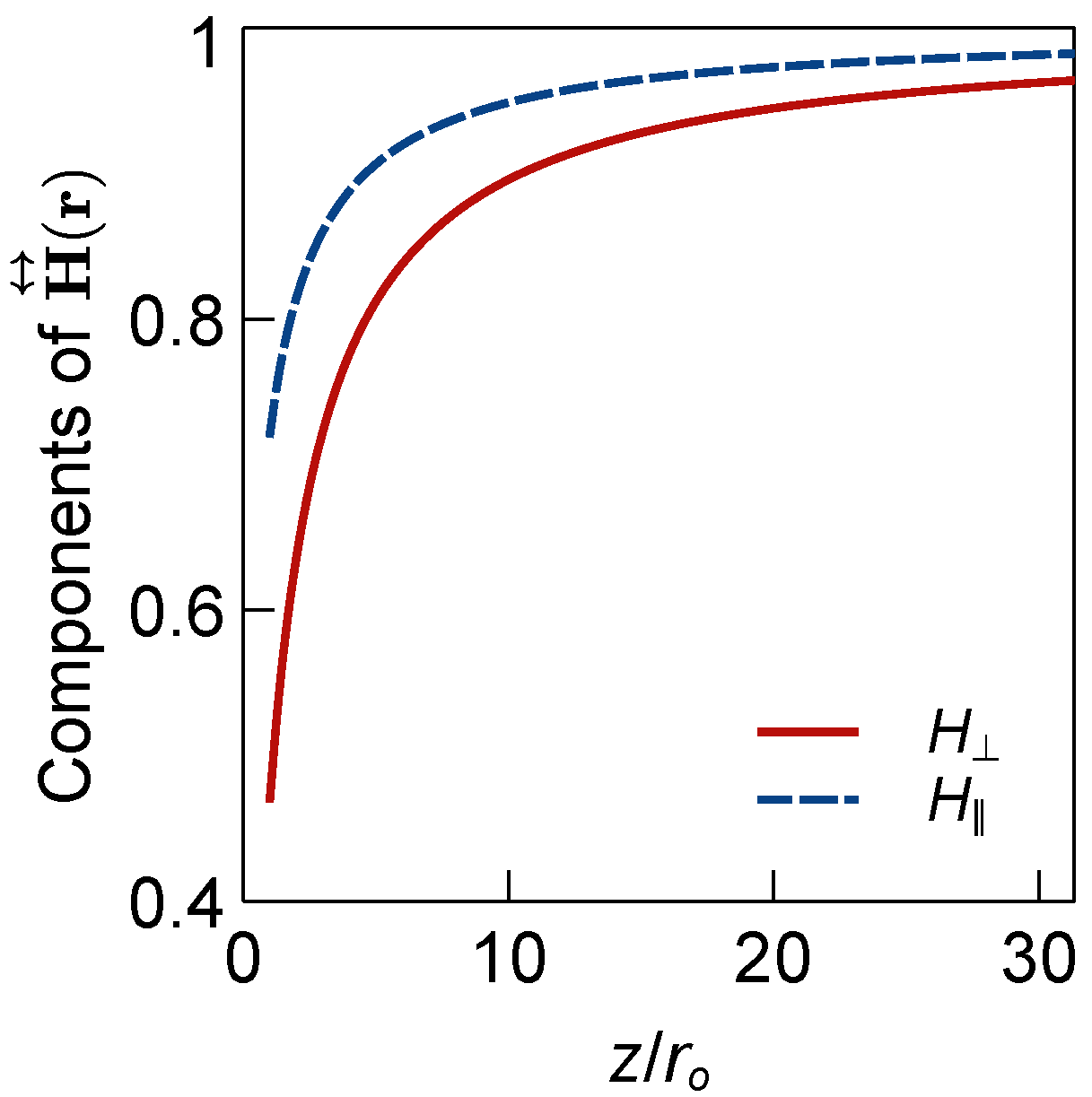
3. Diffusion Tensor and Hydrodynamic Interactions
4. Collision Mechanics
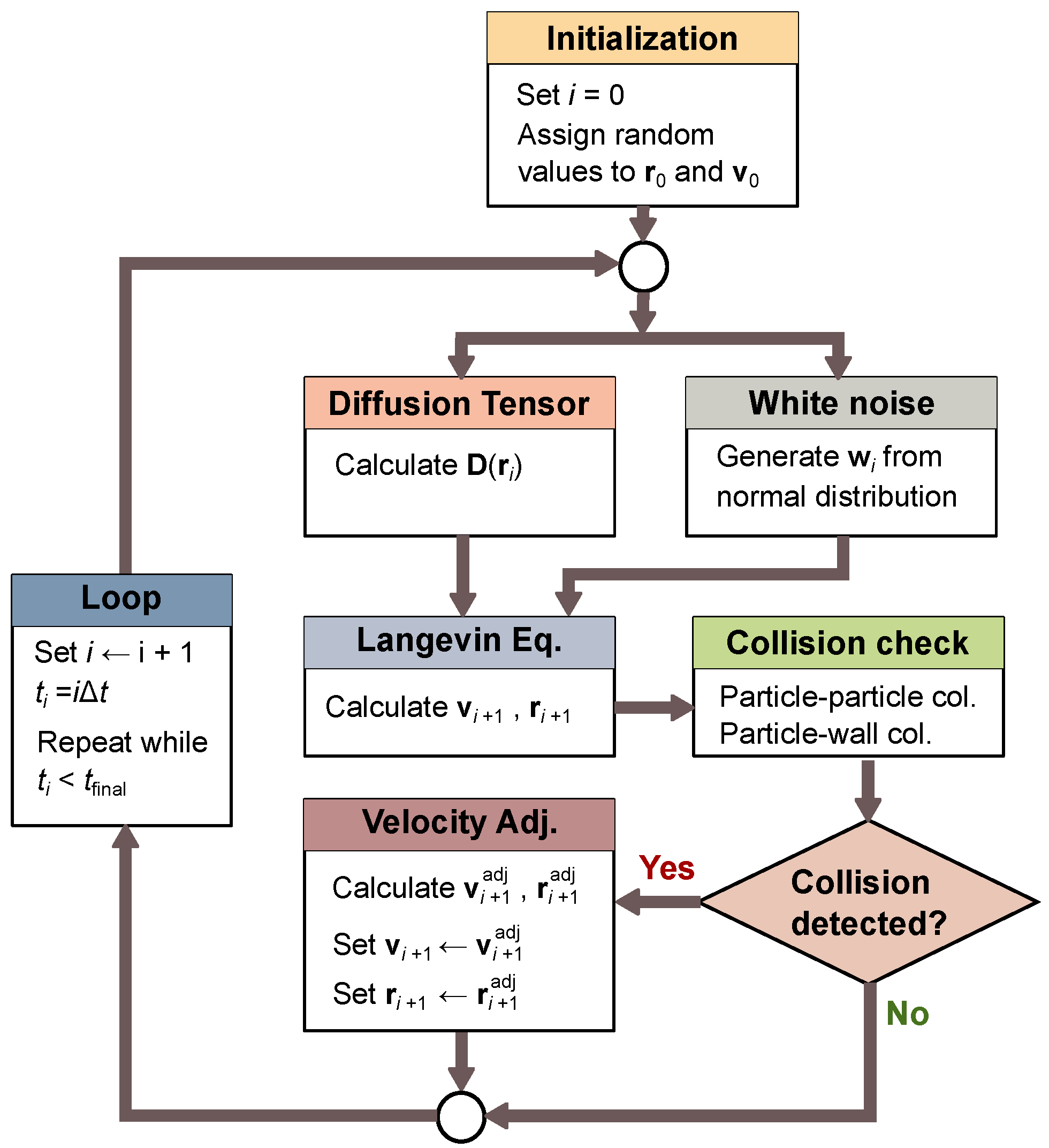
5. Physics Integration
6. Results
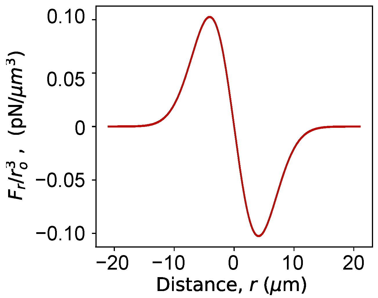
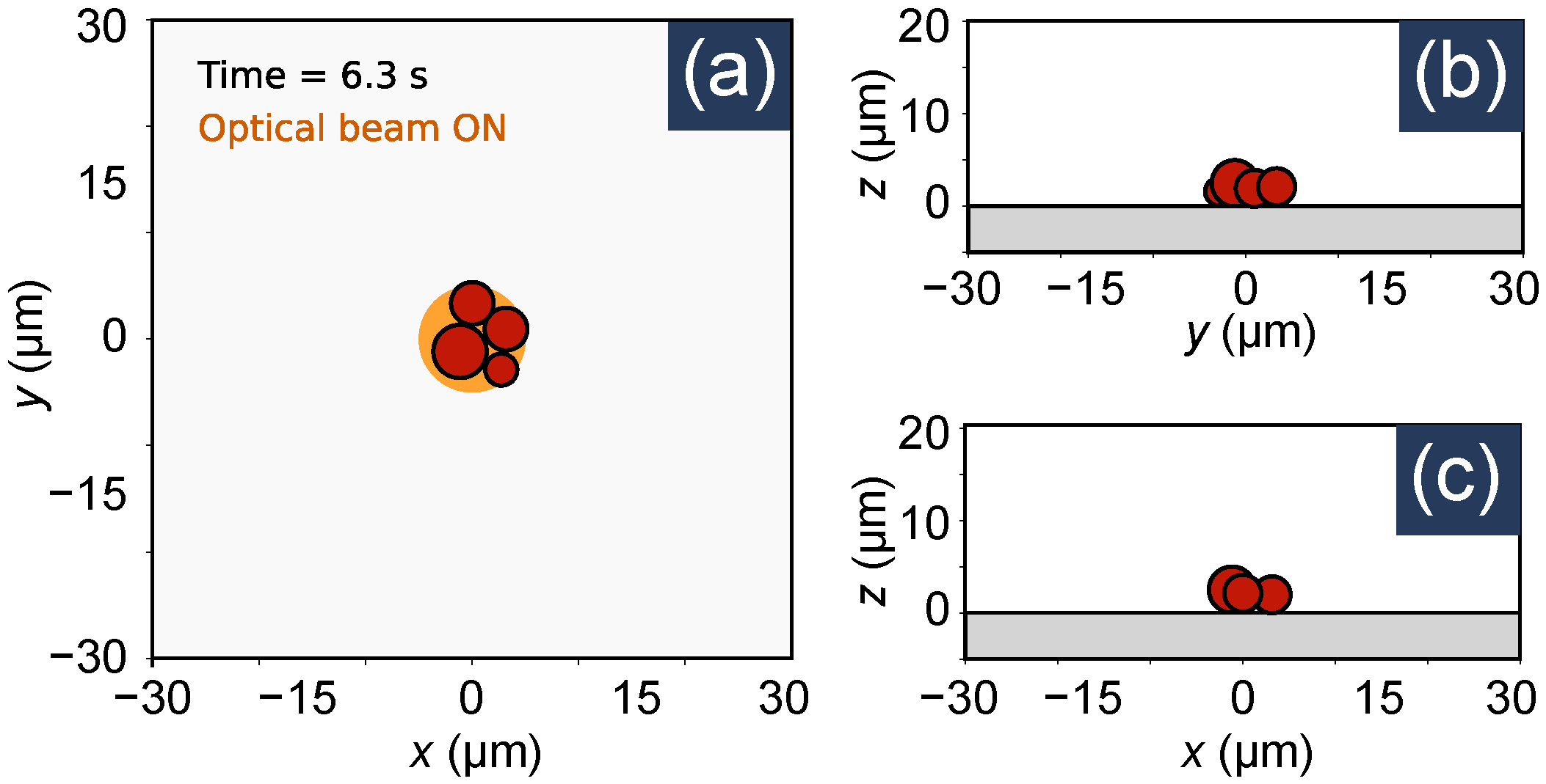
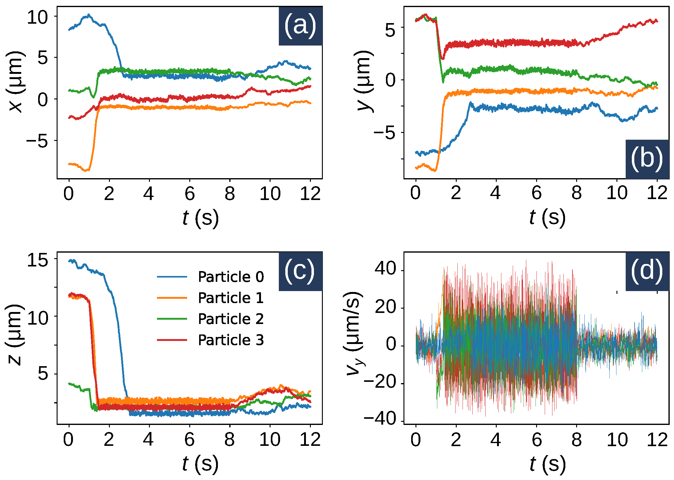
6.1. Optical Trap
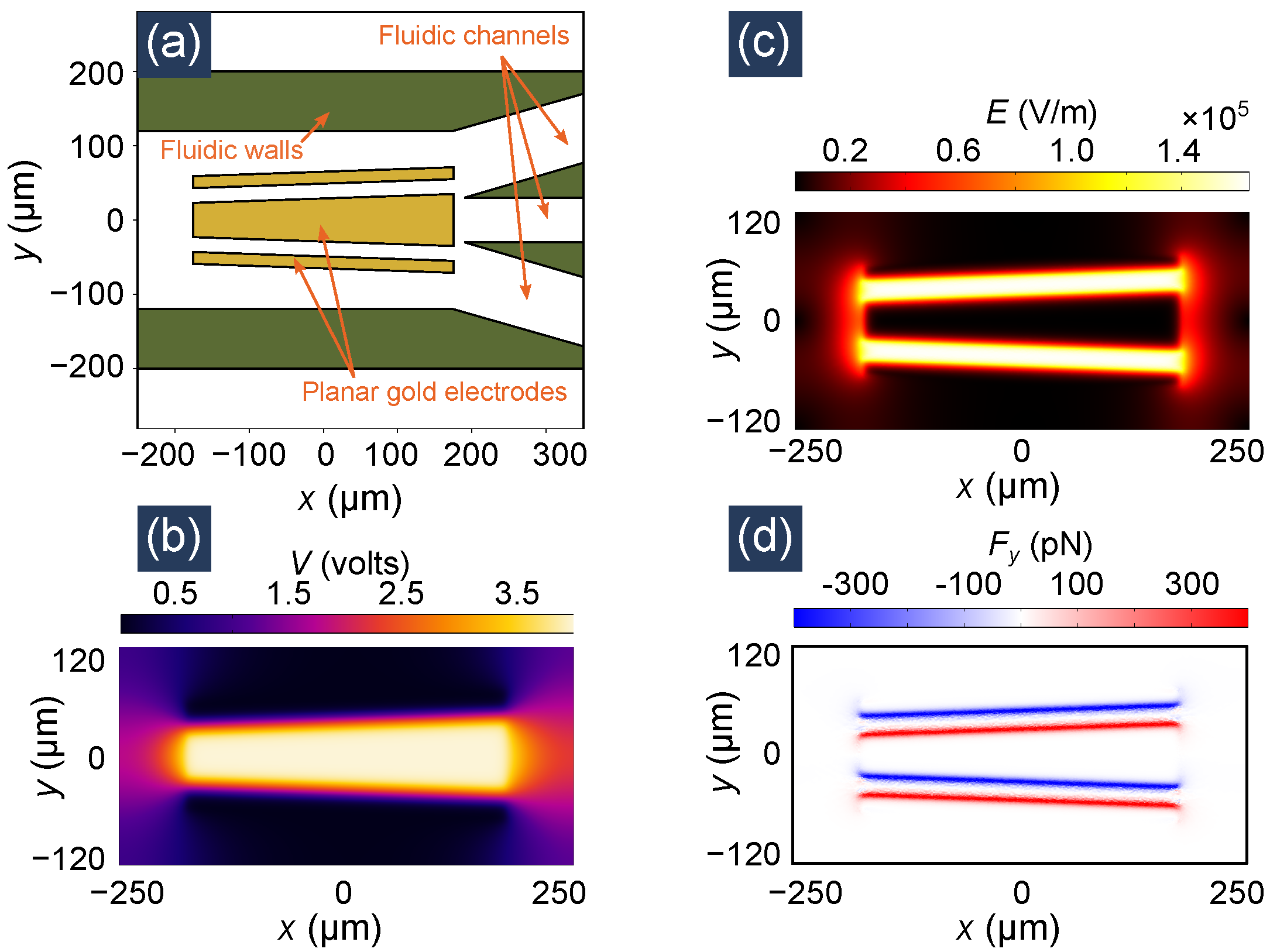
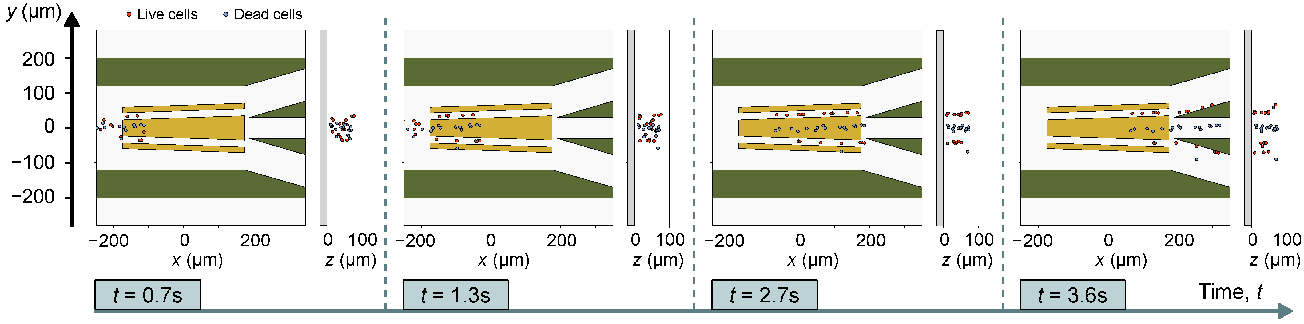
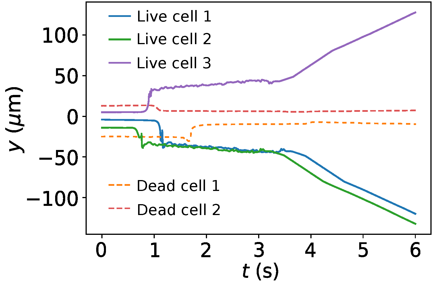
6.2. Dielectrophoretic Cell Sorting or Separation
7. Conclusions
Supplementary Materials
Author Contributions
Funding
Institutional Review Board Statement
Informed Consent Statement
Data Availability Statement
Acknowledgments
Conflicts of Interest
References
- Markarian, N.; Yeksel, M.; Khusid, B.; Farmer, K.R.; Acrivos, A. Particle motions and segregation in dielectrophoretic microfluidics. J. Appl. Phys. 2003, 94, 4160–4169. [Google Scholar] [CrossRef]
- Arefi, S.M.A.; Yang, C.W.T.; Sin, D.D.; Feng, J.J. Simulation of nanoparticle transport and adsorption in a microfluidic lung-on-a-chip device. Biomicrofluidics 2020, 14, 044117. [Google Scholar] [CrossRef]
- Pethig, R. Review Article—Dielectrophoresis: Status of the theory, technology, and applications. Biomicrofluidics 2010, 4, 022811. [Google Scholar] [CrossRef] [Green Version]
- Zaman, M.A.; Padhy, P.; Ren, W.; Wu, M.; Hesselink, L. Microparticle transport along a planar electrode array using moving dielectrophoresis. J. Appl. Phys. 2021, 130, 034902. [Google Scholar] [CrossRef]
- Hyoung Kang, K.; Xuan, X.; Kang, Y.; Li, D. Effects of dc-dielectrophoretic force on particle trajectories in microchannels. J. Appl. Phys. 2006, 99, 064702. [Google Scholar] [CrossRef] [Green Version]
- Enger, J.; Goksör, M.; Ramser, K.; Hagberg, P.; Hanstorp, D. Optical tweezers applied to a microfluidic system. Lab Chip 2004, 4, 196–200. [Google Scholar] [CrossRef] [Green Version]
- Zaman, M.A.; Padhy, P.; Hesselink, L. Near-field optical trapping in a non-conservative force field. Sci. Rep. 2019, 9, 649. [Google Scholar] [CrossRef]
- Lu, D.; Gámez, F.; Haro-González, P. Temperature Effects on Optical Trapping Stability. Micromachines 2021, 12, 954. [Google Scholar] [CrossRef]
- Hsiao, Y.C.; Wang, C.H.; Lee, W.B.; Lee, G.B. Automatic cell fusion via optically-induced dielectrophoresis and optically-induced locally-enhanced electric field on a microfluidic chip. Biomicrofluidics 2018, 12, 034108. [Google Scholar] [CrossRef]
- Wu, M.C. Optoelectronic tweezers. Nat. Photonics 2011, 5, 322–324. [Google Scholar] [CrossRef]
- Zaman, M.A.; Padhy, P.; Cheng, Y.T.; Galambos, L.; Hesselink, L. Optoelectronic tweezers with a non-uniform background field. Appl. Phys. Lett. 2020, 117, 171102. [Google Scholar] [CrossRef]
- Alshareef, M.; Metrakos, N.; Perez, E.J.; Azer, F.; Yang, F.; Yang, X.; Wang, G. Separation of tumor cells with dielectrophoresis-based microfluidic chip. Biomicrofluidics 2013, 7, 011803. [Google Scholar] [CrossRef] [Green Version]
- Patel, S.; Showers, D.; Vedantam, P.; Tzeng, T.R.; Qian, S.; Xuan, X. Microfluidic separation of live and dead yeast cells using reservoir-based dielectrophoresis. Biomicrofluidics 2012, 6, 034102. [Google Scholar] [CrossRef] [PubMed]
- Calero, V.; Garcia-Sanchez, P.; Ramos, A.; Morgan, H. Combining DC and AC electric fields with deterministic lateral displacement for micro- and nano-particle separation. Biomicrofluidics 2019, 13, 054110. [Google Scholar] [CrossRef] [PubMed] [Green Version]
- Doh, I.; Cho, Y.H. A continuous cell separation chip using hydrodynamic dielectrophoresis (DEP) process. Sens. Actuators A Phys. 2005, 121, 59–65. [Google Scholar] [CrossRef]
- Hughes, M.P. Fifty years of dielectrophoretic cell separation technology. Biomicrofluidics 2016, 10, 032801. [Google Scholar] [CrossRef] [Green Version]
- Kazemi, B.; Darabi, J. Numerical simulation of dielectrophoretic particle separation using slanted electrodes. Phys. Fluids 2018, 30, 102003. [Google Scholar] [CrossRef]
- Mathew, B.; Alazzam, A.; Abutayeh, M.; Gawanmeh, A.; Khashan, S. Modeling the trajectory of microparticles subjected to dielectrophoresis in a microfluidic device for field flow fractionation. Chem. Eng. Sci. 2015, 138, 266–280. [Google Scholar] [CrossRef]
- Choi, S.; Lee, W.I.; Lee, G.H.; Yoo, Y.E. Analysis of the Binding of Analyte-Receptor in a Micro-Fluidic Channel for a Biosensor Based on Brownian Motion. Micromachines 2020, 11, 570. [Google Scholar] [CrossRef]
- Volpe, G.; Volpe, G. Simulation of a Brownian particle in an optical trap. Am. J. Phys. 2013, 81, 224–230. [Google Scholar] [CrossRef] [Green Version]
- Reeves, D.B.; Weaver, J.B. Simulations of magnetic nanoparticle Brownian motion. J. Appl. Phys. 2012, 112, 124311. [Google Scholar] [CrossRef]
- Wei, Y.F.; Hsiao, P.Y. Unfolding polyelectrolytes in trivalent salt solutions using dc electric fields: A study by Langevin dynamics simulations. Biomicrofluidics 2009, 3, 022410. [Google Scholar] [CrossRef] [Green Version]
- Banerjee, A.; Kihm, K.D. Experimental verification of near-wall hindered diffusion for the Brownian motion of nanoparticles using evanescent wave microscopy. Phys. Rev. E 2005, 72, 042101. [Google Scholar] [CrossRef]
- Choi, C.; Margraves, C.; Kihm, K. Examination of near-wall hindered Brownian diffusion of nanoparticles Experimental comparison to theories by Brenner (1961) and Goldman et al. (1967). Phys. Fluids 2007, 19, 103305. [Google Scholar] [CrossRef] [Green Version]
- Svoboda, K.; Block, S.M. Biological Applications of Optical Forces. Annu. Rev. Biophys. Biomol. Struct. 1994, 23, 247–285. [Google Scholar] [CrossRef] [PubMed]
- Zaman, M.A. Brownian Dynamics in a Time-Varying Force-Field. 2021. Available online: https://github.com/zaman13/Brownian-dynamics-in-a-time-varying-force-field (accessed on 7 September 2021).
- Ermak, D.L.; McCammon, J. Brownian dynamics with hydrodynamic interactions. J. Chem. Phys. 1978, 69, 1352–1360. [Google Scholar] [CrossRef]
- Katayama, Y.; Terauti, R. Brownian motion of a single particle under shear flow. Eur. J. Phys. 1996, 17, 136–140. [Google Scholar] [CrossRef]
- Drossinos, Y.; Reeks, M.W. Brownian motion of finite-inertia particles in a simple shear flow. Phys. Rev. E 2005, 71, 031113. [Google Scholar] [CrossRef] [Green Version]
- Higham, D.J. An algorithmic introduction to numerical simulation of stochastic differential equations. SIAM Rev. 2001, 43, 525–546. [Google Scholar] [CrossRef]
- Dimits, A.; Cohen, B.; Caflisch, R.; Rosin, M.; Ricketson, L. Higher-order time integration of Coulomb collisions in a plasma using Langevin equations. J. Comput. Phys. 2013, 242, 561–580. [Google Scholar] [CrossRef]
- Cromer, A. Stable solutions using the Euler approximation. Am. J. Phys. 1981, 49, 455–459. [Google Scholar] [CrossRef]
- Čepič, M. Elastic collisions of smooth spherical objects: Finding final velocities in four simple steps. Am. J. Phys. 2019, 87, 200–207. [Google Scholar] [CrossRef]
- Xu, H.; Käll, M. Surface-Plasmon-Enhanced Optical Forces in Silver Nanoaggregates. Phys. Rev. Lett. 2002, 89. [Google Scholar] [CrossRef] [Green Version]
- Neuman, K.C.; Block, S.M. Optical trapping. Rev. Sci. Instrum. 2004, 75, 2787–2809. [Google Scholar] [CrossRef]
- Zaman, M.A.; Padhy, P.; Hansen, P.C.; Hesselink, L. Dielectrophoresis-assisted plasmonic trapping of dielectric nanoparticles. Phys. Rev. A 2017, 95, 023840. [Google Scholar] [CrossRef]
- Zaman, M.A.; Padhy, P.; Hesselink, L. Capturing range of a near-field optical trap. Phys. Rev. A 2017, 96, 043825. [Google Scholar] [CrossRef]
- Vahey, M.D.; Pesudo, L.Q.; Svensson, J.P.; Samson, L.D.; Voldman, J. Microfluidic genome-wide profiling of intrinsic electrical properties in Saccharomyces cerevisiae. Lab Chip 2013, 13, 2754. [Google Scholar] [CrossRef] [PubMed] [Green Version]
- Ettehad, H.M.; Wenger, C. Characterization and Separation of Live and Dead Yeast Cells Using CMOS-Based DEP Microfluidics. Micromachines 2021, 12, 270. [Google Scholar] [CrossRef]
- Talary, M.S.; Burt, J.P.H.; Tame, J.A.; Pethig, R. Electromanipulation and separation of cells using travelling electric fields. J. Phys. D Appl. Phys. 1996, 29, 2198–2203. [Google Scholar] [CrossRef]
- Asami, K.; Hanai, T.; Koizumi, N. Dielectric properties of yeast cells. J. Membr. Biol. 1976, 28, 169–180. [Google Scholar] [CrossRef]
- Green, N.G.; Ramos, A.; González, A.; Morgan, H.; Castellanos, A. Fluid flow induced by nonuniform ac electric fields in electrolytes on microelectrodes. III. Observation of streamlines and numerical simulation. Phys. Rev. E 2002, 66, 026305. [Google Scholar] [CrossRef] [Green Version]


Publisher’s Note: MDPI stays neutral with regard to jurisdictional claims in published maps and institutional affiliations. |
© 2021 by the authors. Licensee MDPI, Basel, Switzerland. This article is an open access article distributed under the terms and conditions of the Creative Commons Attribution (CC BY) license (https://creativecommons.org/licenses/by/4.0/).
Share and Cite
Zaman, M.A.; Wu, M.; Padhy, P.; Jensen, M.A.; Hesselink, L.; Davis, R.W. Modeling Brownian Microparticle Trajectories in Lab-on-a-Chip Devices with Time Varying Dielectrophoretic or Optical Forces. Micromachines 2021, 12, 1265. https://doi.org/10.3390/mi12101265
Zaman MA, Wu M, Padhy P, Jensen MA, Hesselink L, Davis RW. Modeling Brownian Microparticle Trajectories in Lab-on-a-Chip Devices with Time Varying Dielectrophoretic or Optical Forces. Micromachines. 2021; 12(10):1265. https://doi.org/10.3390/mi12101265
Chicago/Turabian StyleZaman, Mohammad Asif, Mo Wu, Punnag Padhy, Michael A. Jensen, Lambertus Hesselink, and Ronald W. Davis. 2021. "Modeling Brownian Microparticle Trajectories in Lab-on-a-Chip Devices with Time Varying Dielectrophoretic or Optical Forces" Micromachines 12, no. 10: 1265. https://doi.org/10.3390/mi12101265