Analysis of Electrokinetic Mixing Techniques Using Comparative Mixing Index

Abstract
:1. Introduction
2. Comparative Mixing Index (CMI)
3. Mathematical Model

| Parameter | Value | Description |
|---|---|---|
| W | 100 µm | Width of the microchannel |
| Lc | 2 mm | Length of microchannel |
| ϛf | −50 mv | Fixed zeta potential on channel walls |
| Ds | 5e−11 m2/s | Diffusivity of species to be mixed |
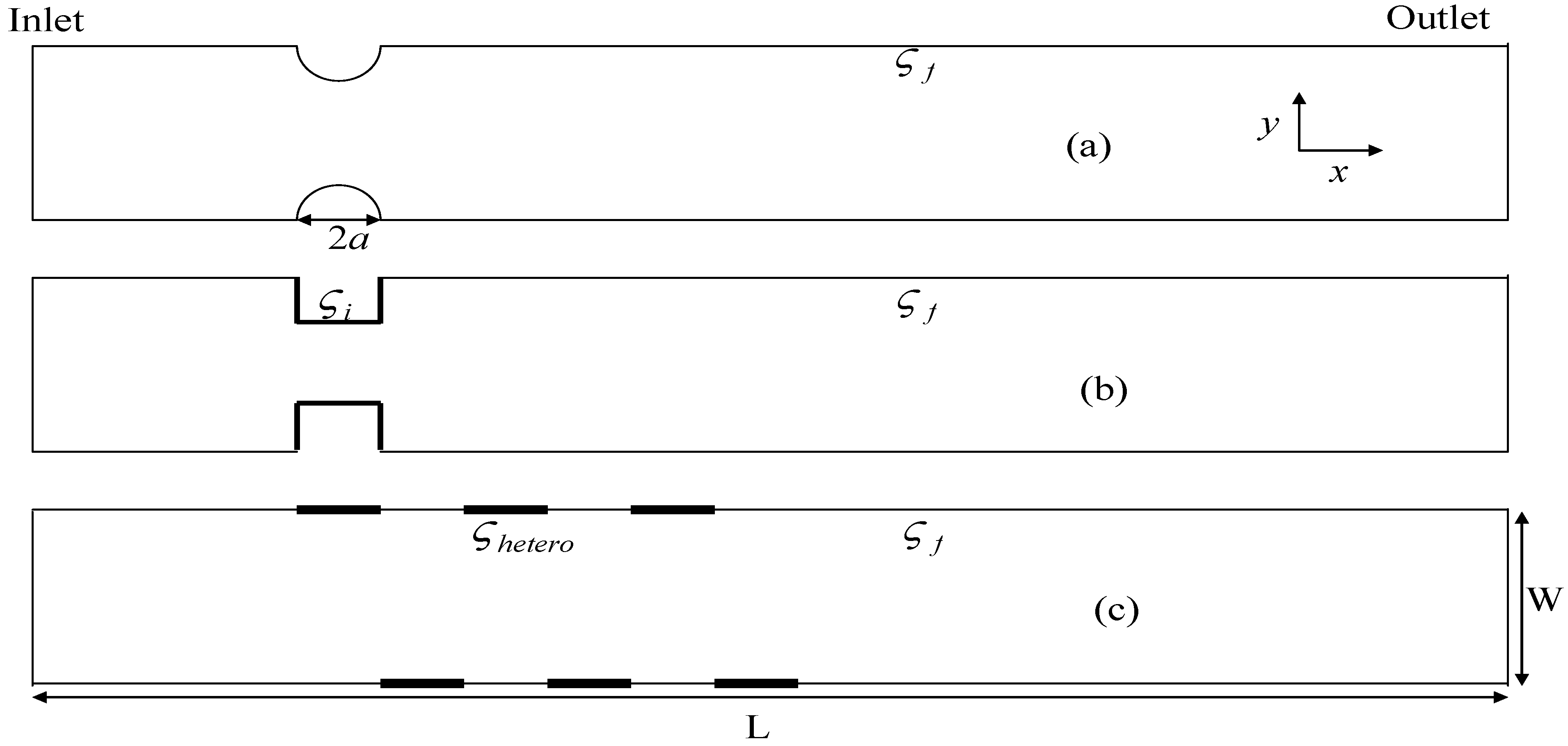
| a | 25 µm | Radius of non-conducting obstacle (Figure 2) |
| p | 100 µm | Heterogeneous charged surface patch length (Figure 5) |
4. Results and Discussion

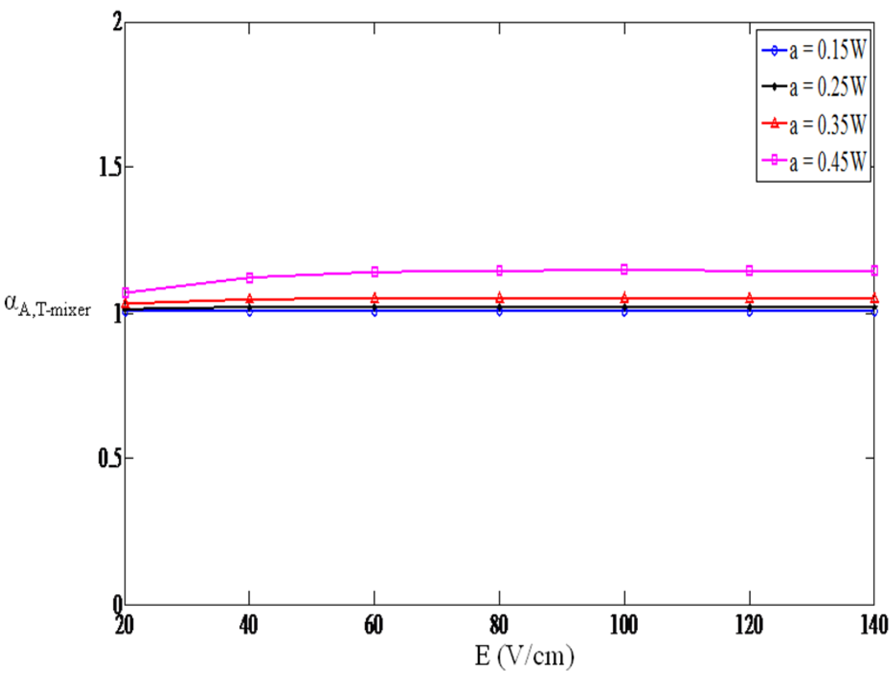
4.1. Physical Constriction / Obstacle Based Mixer


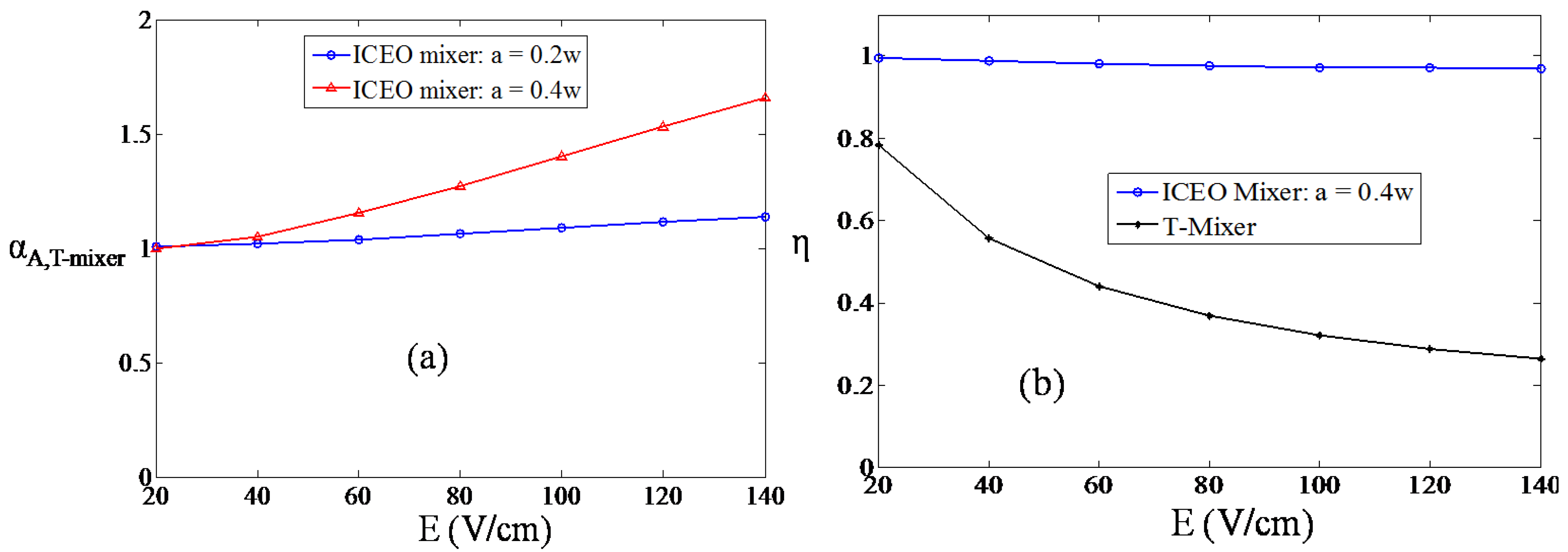
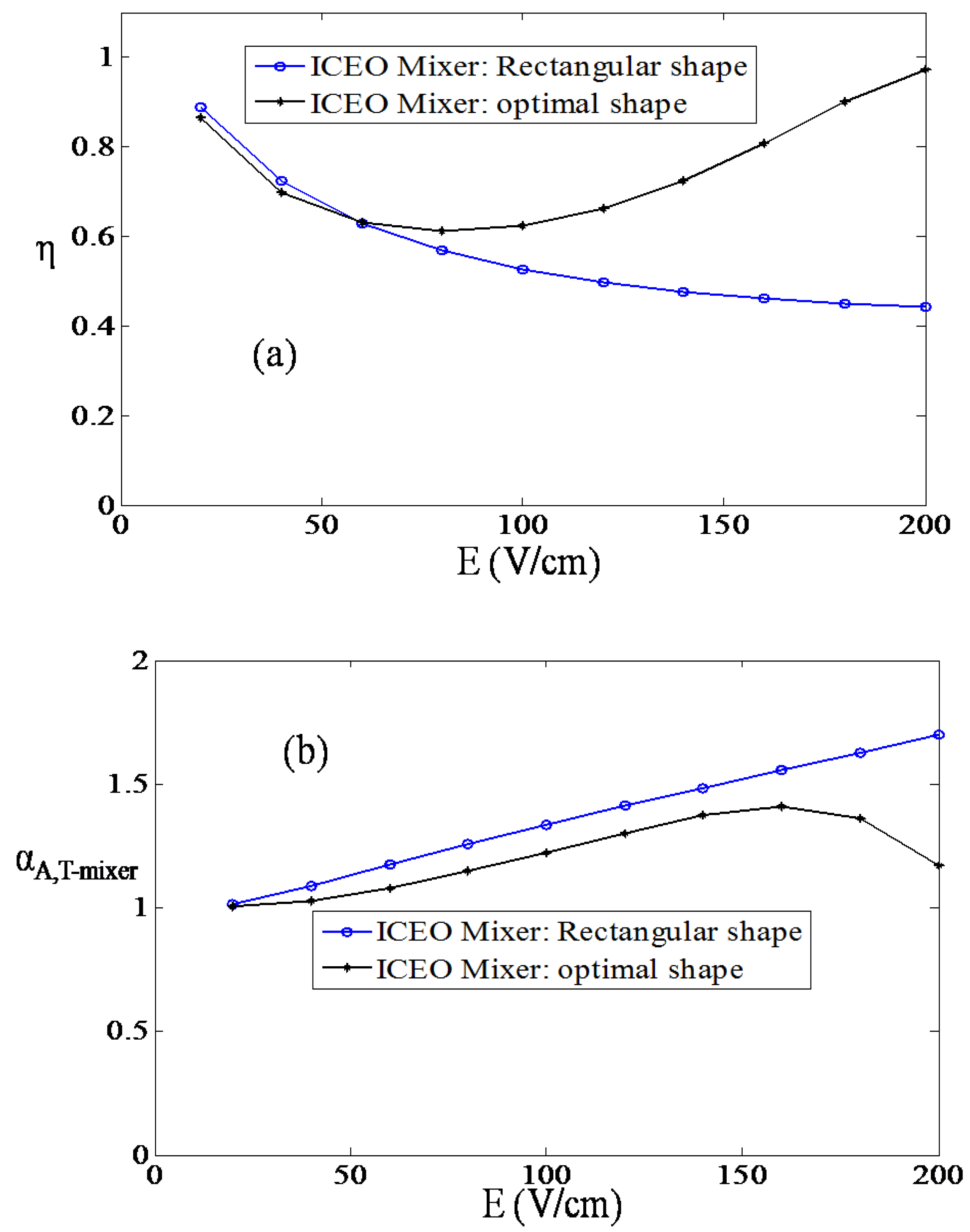
4.2. Induced Charge Electro-osmotic (ICEO)/ Conducting Obstacle Mixer


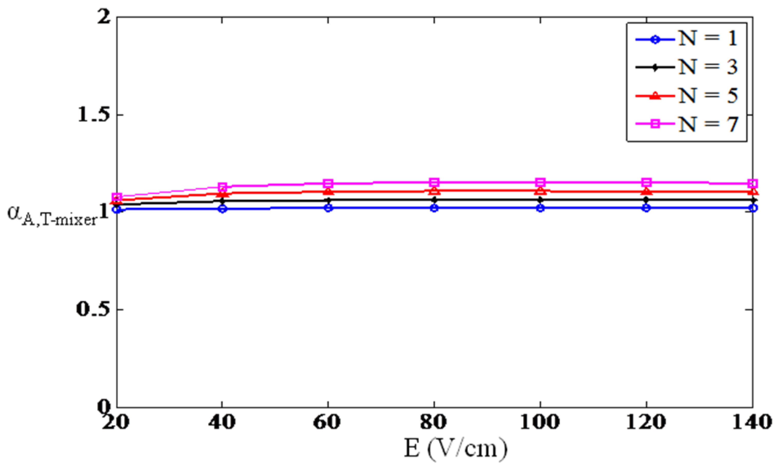
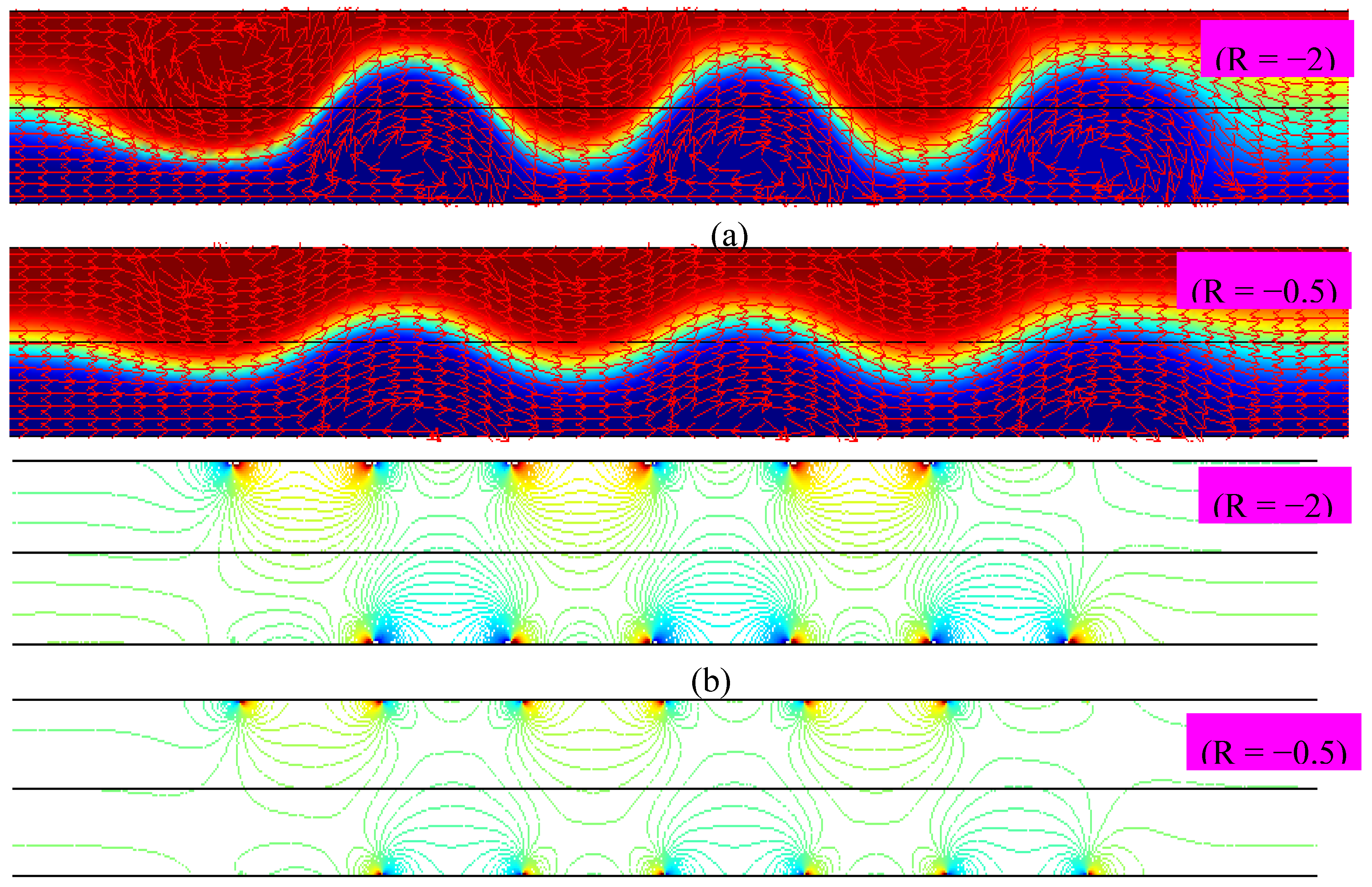
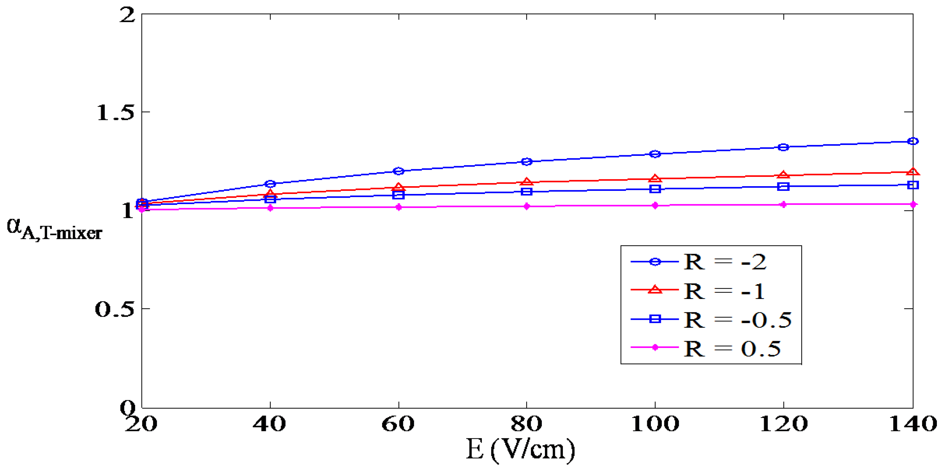
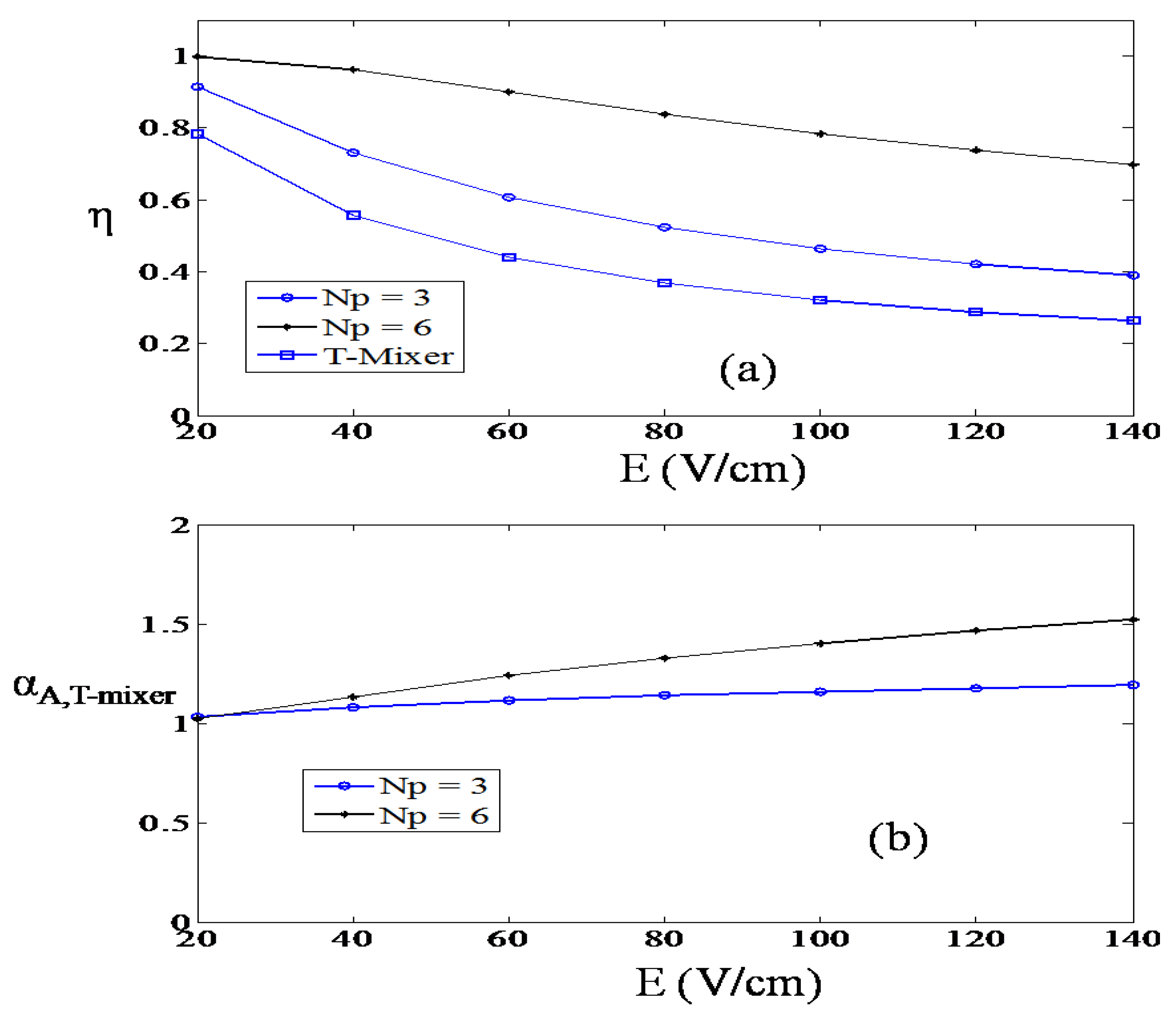
4.3. Heterogeneously Charged Walls Mixer


5. Conclusions
References
- Nguyen, N.T.; Wu, Z.G. Micromixers—A review. J. Micromech. Microeng. 2005, 15, R1–R16. [Google Scholar]
- Chang, C.C.; Yang, R.J. Electrokinetic mixing in microfluidic systems. Microfluid. Nanofluid. 2007, 3, 501–525. [Google Scholar] [CrossRef]
- Coleman, J.T.; Sinton, D. A sequential injection microfluidic mixing strategy. Microfluid. Nanofluid. 2005, 1, 319–327. [Google Scholar] [CrossRef]
- Biddiss, E.; Erickson, D.; Li, D. Heterogeneous surface charge enhanced micromixing for electrokinetic flows. Anal. Chem. 2004, 76, 3208–3213. [Google Scholar] [PubMed]
- Stroock, A.D.; Dertinger, S.K.W.; Ajdari, A.; Mezic, I.; Stone, H.A.; Whitesides, G.M. Chaotic mixer for microchannels. Science 2002, 295, 647–651. [Google Scholar] [CrossRef] [PubMed]
- Oddy, M.H.; Santiago, J.G.; Mikkelsen, J.C. Electrokinetic instability Micromixing. Anal. Chem. 2001, 73, 5822–5832. [Google Scholar] [CrossRef] [PubMed]
- Wu, Z.; Li, D. Mixing and flow regulating by induced-charge electrokinetic flow in a microchannel with a pair of conducting triangle hurdles. Microfluid. Nanofluid. 2008, 5, 65–76. [Google Scholar] [CrossRef]
- Wu, Z.; Li, D. Micromixing using induced-charge electrokinetic flow. Electrochim. Acta 2008, 53, 5827–5835. [Google Scholar] [CrossRef]
- Jain, M.; Yeung, A.; Nandakumar, K. Efficient micromixing using induced-charge electroosmosis. J. Microelectromech. Syst. 2009, 18, 376–384. [Google Scholar] [CrossRef]
- Jain, M.; Yeung, A.; Nandakumar, K. Induced charge electro osmotic mixer: Obstacle shape optimization. Biomicrofluidics 2009, 3, 022413. [Google Scholar] [CrossRef]
- Chang, C.C.; Yang, R.J. Computational analysis of electrokinetically driven flow mixing in microchannels with patterned blocks. J. Micromech. Microeng. 2004, 14, 550–558. [Google Scholar] [CrossRef]
- Chen, C.K.; Cho, C.C. Electrokinetically-driven flow mixing in microchannels with wavy surface. J. Colloid Interface Sci. 2007, 3, 470–480. [Google Scholar] [CrossRef]
- Tian, F.Z.; Li, B.M.; Kwok, D.Y. Tradeoff between mixing and transport for electroosmotic flow in heterogeneous microchannels with nonuniform surface potentials. Langmuir 2005, 21, 1126–1131. [Google Scholar] [CrossRef]
- Jain, M.; Nandakumar, K. Novel index for micromixing characterization and comparative analysis. Biomicrofluidics 2010, in press. [Google Scholar]
- Hunter, R.J. Zeta Potential in Colloid Science: Principals and Applications; Academic Press Inc.: New York, NY, USA, 1981. [Google Scholar]
- Squires, T.M.; Bazant, M.Z. Induced-charge electro-osmosis. J. Fluid Mech. 2004, 509, 217–252. [Google Scholar] [CrossRef]
- Erickson, D.; Li, D. Influence of surface heterogeneity on electrokinetically driven microfluidic mixing. Langmuir 2002, 18, 1883–1892. [Google Scholar] [CrossRef]
© 2010 by the authors; licensee MDPI, Basel, Switzerland. This article is an open access article distributed under the terms and conditions of the Creative Commons Attribution license (http://creativecommons.org/licenses/by/3.0/).
Share and Cite
Jain, M.; Yeung, A.; Nandakumar, K. Analysis of Electrokinetic Mixing Techniques Using Comparative Mixing Index. Micromachines 2010, 1, 36-47. https://doi.org/10.3390/mi1020036
Jain M, Yeung A, Nandakumar K. Analysis of Electrokinetic Mixing Techniques Using Comparative Mixing Index. Micromachines. 2010; 1(2):36-47. https://doi.org/10.3390/mi1020036
Chicago/Turabian StyleJain, Mranal, Anthony Yeung, and Krishnaswamy Nandakumar. 2010. "Analysis of Electrokinetic Mixing Techniques Using Comparative Mixing Index" Micromachines 1, no. 2: 36-47. https://doi.org/10.3390/mi1020036