Evolutionary Multi-Objective Energy Production Optimization: An Empirical Comparison


1
Artificial Intelligence Research Center, University of Veracruz, Sebastián Camacho 5, Col. Centro, Xalapa 91000, Veracruz, Mexico
2
Naturally Inspired Computation Research Group, Department of Computer Science, Maynooth University, Maynooth W23 F2K8, Kildare, Ireland
*
Author to whom correspondence should be addressed.
Math. Comput. Appl. 2020, 25(2), 32; https://doi.org/10.3390/mca25020032
Submission received: 21 April 2020
/
Revised: 12 June 2020
/
Accepted: 15 June 2020
/
Published: 16 June 2020
(This article belongs to the Special Issue New Trends in Computational Intelligence and Applications)
Abstract
:This work presents the assessment of the well-known Non-Dominated Sorting Genetic Algorithm II (NSGA-II) and one of its variants to optimize a proposed electric power production system. Such variant implements a chaotic model to generate the initial population, aiming to get a better distributed Pareto front. The considered power system is composed of solar, wind and natural gas power sources, being the first two renewable energies. Three conflicting objectives are considered in the problem: (1) power production, (2) production costs and (3) CO2 emissions. The Multi-Objective Evolutionary Algorithm based on Decomposition (MOEA/D) is also adopted in the comparison so as to enrich the empirical evidence by contrasting the NSGA-II versions against a non-Pareto-based approach. Spacing and Hypervolume are the chosen metrics to compare the performance of the algorithms under study. The obtained results suggest that there is no significant improvement by using the variant of the NSGA-II over the original version. Nonetheless, meaningful performance differences have been found between MOEA/D and the other two algorithms.
1. Introduction
Climate change is a very relevant problem that human kind is facing. The United Nations Organization has warned that approximately a dozen years are left to limit climate change at 1.5 °C in order to prevent a world crisis [1]. Power production is one of the key elements to consider. Fossil fuels have been and continue to be widely used to produce electricity. These energy sources, when burned to generate heat to produce power, emit nitrogen oxides and other pollutants that contribute to the smog and acid rain [2]. Several countries, including the United States (US), have started to adopt renewable energy sources, such as solar and wind energy, to produce electric power. In 2017, around 11% of the total consumed energy in the US came from renewable energies [3], equivalent to approximately 11 quadrillion British Thermal Units (Btu). Moreover, about 17% of the generated electricity alone was from renewables.
Even though the government has encouraged the transition to cleaner energy sources, fossil fuels such as oil, coal and natural gas are still widely used. The US Energy Information Administration (EIA) states that 77.6% of the total produced energy in the country in 2017 came from the three aforementioned energy sources [3], where the latter is the most utilized.
With respect to the state of Oklahoma, according to the US Department of Energy [4], 50% of the annual energy production in 2016 came from natural gas, 38% from coal and only 10% came from solar and wind power and 1% from hydro-energy. Moreover, the annual consumed energy, equivalent to near 59.3 TWh, represents the 2% of the total consumption in the US. Despite the US government position about climate change, as indicated in [5], the renewable energy industry is expected to grow and play an important role in the energy production, not only in Oklahoma, but in some of the most populated states of the country.
Renewable energy production in the state of Oklahoma is low compared to the employment of fossil fuels, nonetheless, transition to renewable energy is promising. The American Wind Energy Association (AWEA) establishes that Oklahoma has the 4th rank among all the states for the number of wind turbines. Furthermore, it has the 2nd rank for the total installed wind capacity [6]. As for solar power, Oklahoma has the 6th rank in solar power potential, being said that solar energy could provide up to 44.1% of all the required electricity [7].
For better care of the environment as well as for better use of limited resources, the use of solar and wind power is highly recommended. As the transition to entirely renewable source-based power production systems may be achieved in a gradual and slow fashion, natural gas is still considered to be used for the purposes of this paper.
Beyond the merely direct utilization of these power sources, an optimal distribution of the generation power among the three is highly desirable. Power production systems usually deal with more than one target to fulfill conflicting requirements. From that standpoint, the power production becomes a Multi-objective Optimization problem. Different metaheuristics have been applied in the context of power systems optimization. Swarm Intelligence algorithms have been used in the past, e.g., Particle Swarm Optimization (PSO) is applied for the multi-objective planning of power distribution [8], where the authors proposed a novel method of selection based on non-dominated solutions and the dominated fittest solutions. Differential Evolution (DE) has also been employed in the context of power systems [9], where a multi-objective DE algorithm is used to maximize hydroelectric power production while minimizing the annual deficit of irrigation. Artificial Bee Colony (ABC) algorithm is used in its multi-objective variant to solve a power flow problem [10]. Total fuel cost, power losses, voltage profiling, voltage stability and total emissions are the chosen objective functions in this work. More recently, new metaheuristics have also been adopted. A variant of the Pigeon-Inspired Algorithm is implemented in [11], where the authors aim to maximize the short-term hydropower generation in a cascade setting, basing on the height of the water flow stream and the total flow as decision variables. In [12], a parallel implementation of metaheuristics is used to train the weights of an Artificial Neural Network (ANN) to predict wind power. The authors introduced several communication schemes among threads, i.e., each thread representing a part of the population. Multi-objective Evolutionary Algorithms (MOEA) are also useful to solve these types of problems and an important branch of these algorithms have been developed. The algorithm of interest in this work is the well known Non-Dominated Sorting Genetic Algorithm II (NSGA-II) [13], which has been a popular choice to solve multiple multi-objective optimization problems, in general, and multi-objective power optimization problems, in particular.
Wahlroos, Jaaskelainen and Hirvonen [14] optimized a generation system in terms of CO2 emissions, production costs and production adequacy, using the aforementioned algorithm. Wang and Zhou [15] utilized the same algorithm to optimize the emissions and energy-savings of a wind power system. Liu and Dongdong [16] optimized a multiple-source power system considering its production cost and the amount of emissions it produces. Zhou and Sun [17] utilized NSGA-II to optimize a hybrid energy system consisting of solar and wind power. All these works demonstrate the positive impact that NSGA-II has in these type of energy-based problems. For this study, the results yielded by NSGA-II, as well as the results obtained by MOEA/D, are compared with a modified version of this popular algorithm, called L-NSGA-II, proposed by Liu et al. [18].
Motivated by the aforementioned works, and particularly by the works carried out by Zhou and Sun [17] and Liu et al. [18], the contributions of this work are: (1) the statement of a novel Multi-Objective Optimization problem based on the Oklahoma power production, and (2) its resolution by using NSGA-II and one of its variants (L-NSGA-II) with the aim of assessing their performance in this new real-world instance. The results are further compared against a representative MOEA based on decomposition, i.e., MOEA/D.
The optimization problem is based on three objective functions: (1) produced power, (2) production costs and (3) CO2 emissions. These functions depend on four real-domain variables: hours of operation of solar power (), wind power (), and natural gas power (), and the amount of natural gas power to be produced (). The hours of operation are constrained to a minimum of 240 h and a maximum of 672 h each, equivalent to 10 days and 28 days, respectively. Natural gas power production is bounded to the range of 4.88 MW to 7.07 MW. More detail of the system configuration is provided in Section 6.
The rest of this paper is organised as follows. Section 2 discusses the main elements of the energy sources treated in this work along with some properties. Section 3 formally describes the problem used in this study. Section 4 presents the climate model adopted and Section 5 introduces the multi-objective optimization evolutionary algorithms (MOEAs) assessed in this study. The experimental setup is shown in Section 6. Section 7 presents the results obtained by the MOEAs and discusses such results. Finally, Section 8 concludes this paper.
2. Energy Sources
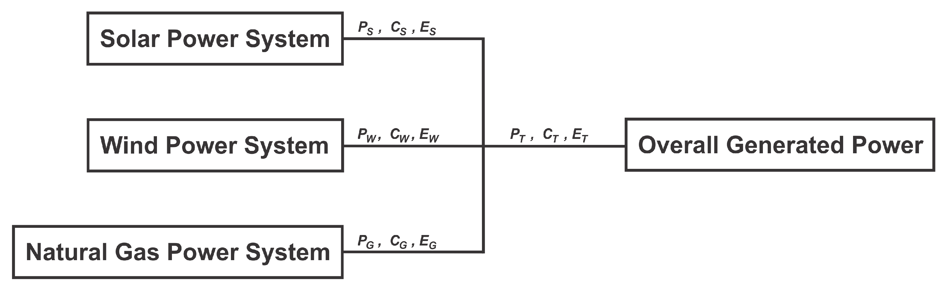
The proposed power production system, as previously mentioned, is based on solar, wind, and natural gas energy. They are the most feasible, less polluting power sources in the state of Oklahoma. Next, we define some elements along with some properties that are essential for the optimization problem at hand. A very general schematic of the described power system is shown in Figure 1.
2.1. Solar Power
Solar energy is obtained from solar radiation coming directly from solar rays. The Office of Energy Efficiency and Renewable Energy of the US defines it as any kind of electromagnetic radiation coming from the sun [19]. This energy source can be used to generate electric power. The Watt (W) is the International System unit to measure the solar radiation. When measured with respect to certain surface of concentration, the unit transforms into W/m2.
2.2. Wind Power
The wind power generation is more complex, as the main input is the wind speed. This carries kinetic energy which is converted to electric power [20].
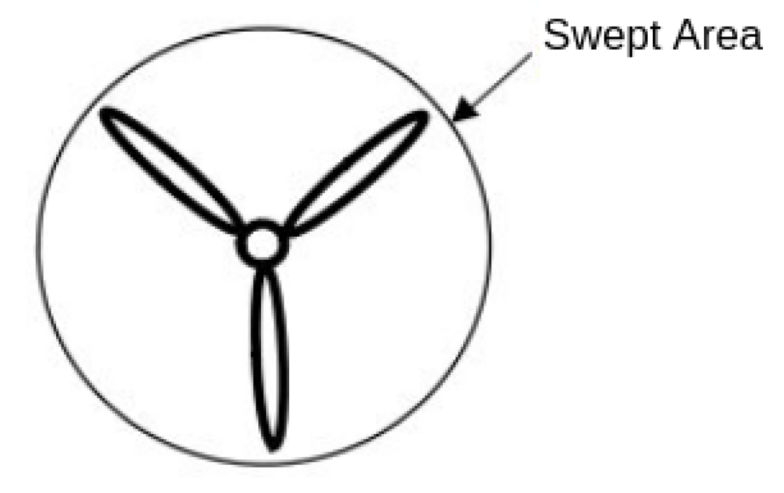
The conversion equipment for wind power is the wind turbine. It possesses a certain number of blades attached to a rotor. Usually, three blades configuration is used. Figure 2 shows the basic configuration of a wind turbine.
The swept area, shown in Figure 2, is the imaginary contour traveled by the blades. The ideal wind power is calculated using Equation (1):
where is the generated wind power measured in watts, A is the swept area, which depends on the length of the blades. The constant is the air density, assumed to be 1.23 Kg/m3 and V is the wind speed, measured in m/s.
For both, solar and wind energy, the Wh (Watt-hour) is another common energy unit. It represents the total number of Watts sustained per hour.
2.3. Capacity Factor
Solar radiation and wind power, computed using Equation (1), correspond to the maximum possible amounts of power. Normally, the amount of produced power tends to be less than the calculated power. For natural gas power, whose generation is not studied here, there also exists a real amount of power that differs from theoretical expectations.
The capacity factor is the ratio of the net generated power to the maximum possible power output that could have been generated, both for a considered period of time [21]. The capacity factors for solar, wind, and natural gas power are defined and showed in Table 1.
It can be seen that natural gas energy has a higher availability. Solar power is the less productive out of the three power sources. In spite of the low capacity factors found in solar and wind systems, new technologies might emerge in order to better benefit from these renewable sources.
2.4. Production Cost
Costs of production are inherent to the power systems. Solar, wind and natural gas power systems represent different costs, which increase as the number of hours of operation do as well.
The production cost is the measurement of how much it costs to produce a Wh of energy. Large scale production might use the $/MWh as measurement unit. The production costs of the three analyzed energy sources are shown in Table 2.
With respect to the costs shown in Table 2, natural gas power shows the best performance, being the most cost-effective energy source. Solar power is the most expensive; more hours of operation are needed in pursuance of producing the same amount of power than, for example, wind energy. Both, Table 1 and Table 2, have been gathered from [22].
2.5. CO2 Emissions Rate
The last consideration for power production, and becoming increasingly important in recent years, is its environmental impact. Every power production system entails emissions of carbon dioxide (CO2). The National Aeronautics and Space Administration (NASA) states that CO2 is one of the most important contributors to global warming [23].
Each power system’s performance is also measured with respect to how many grams or kilograms of CO2 they produce per Watt or Watt-hour. These emissions are referred as CO2 emissions rate. For this work, the emission rates are measured in gr/KWh. Emissions rates are shown in Table 3.
Natural gas greatly surpasses both, solar and wind energy with the highest emissions rate. This makes natural gas the most polluting energy source, out of the presented list.
3. Optimization Problem
A multi-objective optimization problem can be defined, without loss of generality, as to find a solution vector , which minimizes the set of functions , where each variable . There are n decision variables comprised in . The terms lo and up represent the lower and upper bound of a variable, respectively. The m objective functions are usually conflicting with each other. That is, a solution modification leads to improved performance in one objective and worsened performance in another objective.
Pareto dominance is used as a criterion to solve multi-objective optimization problems. In the context of minimization, a multi-objective problem is defined as follows: a solution vector is said to dominate , denoted as , if and only if, for all and for at least one .
A solution vector is part of the Pareto Optimal Set if there does not exist other solution such that . The Pareto Optimal Front is then .
The analyzed power production system, as previously mentioned, is based on solar, wind, and natural gas energy. Three objective functions are considered: (1) the overall power production, (2) the overall production cost, and (3) the overall CO2 emissions. Four decision variables are contemplated in this study. The first three variables are the hours of operation of each system, referred as , , and . The fourth variable is the amount of energy produced by the natural gas system alone, .
In order to ensure the conflicting nature between functions, another important assumption is introduced to the power system model. Currently, the power capacity in Oklahoma is installed, which favors the reduction in costs of production while maintaining operations. For the purposes of this work, the power system capacity is considered yet to be installed. Under this supposition, and based on some of the objective functions presented in [24], this multi-objective optimization scenario is possible.
3.1. Power Production Function
The first objective function (P) formally formulated in Equation (2), presents the entire monthly amount of power produced by the three sources:
where , highlighted in bold, are decision variables. and are the estimations of the input solar and wind power, respectively, for any arbitrary month coming from the respective energy sources. is the generated natural gas power. and depend entirely on climate conditions (as explained in a later section) and in this application scenario, is assumed to be provided as much as needed, therefore becoming a decision variable. Constants , and are the capacity factors of solar, wind and natural gas sources, respectively (see Table 1).
It is imperative to note that the power production function is to be maximized, however, the algorithms that will be soon explained are set to minimize the objectives. The relevance of the maximization of the function in Equation (2) lies in the nature of this application problem; as the power system installation depends on weather conditions, maximizing the generated power aids on securing power supply. For simplification, generation-demand balance has been overlooked. For this matter, this target function is transformed using the concept of power relation, mathematically expressed in Equation (3).
where is the current monthly amount of produced energy, for August 2018, in the state of Oklahoma, equivalent to approximately 7.07 thousand MWh [25]. N is an increasing factor constant. In an ideal context, where renewable power is reinforced, the increasing factor is greater than one. Thereby, the total energy from solar, wind, and natural gas is forced to increase. For this study, the total power production is encouraged to be doubled, thus . By allocating the overall power production function (see Equation (2)) in the denominator, its maximization is assured, as the only way to minimize the power relation is to maximize its denominator. Using this new objective function leads the algorithm to reach a produced power amount at least as high as twice the current produced power . As it was mentioned earlier, the power system model assumes that the power capacity is yet to be installed, thus the maximization of the power generation is reliable, taking into account the other two objective functions.
3.2. Production Cost Function
The second objective function (C) represents the total monthly production cost. Equation (4) formally expresses this objective to be minimized,
where constants , and are the production costs of solar, wind, and natural gas systems, respectively (see Table 2). The rest of the variables are those defined previously.
3.3. CO2 Emissions Function
The third objective function (E) is the monthly CO2 emissions caused by the three energy sources. This objective function is to be minimized, as formally formulated in Equation (5).
where , and are CO2 emissions rates for solar, wind, and natural gas systems, respectively (see Table 3).
Moura and de Almeida [24] employed a similar optimization framework for a power system in Portugal, using comparable objective functions, which inspired our functions’ design. Given the aforementioned objective functions and the decision variables, the multi-objective optimization problem is now stated as: to find the vector , which minimizes the set of functions , where and .
The objective functions previously defined differ from the background research formerly presented. In [14], the energy optimization system consisted on electricity and heat generation as the two objective functions, and the production was distributed between them. In [15], the authors optimized the energy costs and CO2 and SO2 emissions for a wind energy system. Their three objective functions were constrained with respect to the wind power output. The authors of [16] proposed a multi-energy system to be optimized where two objective functions were introduced: (1) daily operation costs and (2) emissions. Their energy system takes into account natural gas power and electricity. In [17], the authors optimized the power generation costs of solar power and wind power, where these two power sources are adversaries between each other. Finally, the work in [18] optimizes production wasting and power consumption as the objective functions, in a process of natural gas and oil power generation. Considering the fact that these power systems are not equal as the system we proposed in this research, the objective functions used in this paper are significantly different as well.
4. Climate Model
As mentioned before, solar and wind power depend on solar radiation and wind speed, respectively. Unfortunately, these two variables are highly reliant on weather. This work aims to optimize the power production system for each month of each year from 2020 to 2025, thus a prediction approach is required.
It is well known that predicting climate is an incredibly challenging task. Moura and de Almeida proposed a climate model prediction for Portugal, based on previous data [24]. A similar model is implemented for the state of Oklahoma. A dataset is built with measurements of solar radiation and wind speeds for each month of each year from 2003 to 2017, provided by MESONET, an environmental monitoring network in the state of Oklahoma [26].
The solar radiation measured by MESONET is given in MJ/m2. In order to match with the previously commented units, measurements are converted to Watts, by multiplying the data by the equivalent area of all the available solar panels and dividing it by the total number of seconds in each month. Twenty thousand solar panels are considered for this study, each having an area of 1.65 m2, which is a common commercial surface. The number of seconds per month is calculated depending on whether a month has 28, 30 or 31 days. The wind speed is measured in miles per hour and only needs to be converted to m/s.
The average solar radiation and average wind speed are computed for each month, as well as standard deviations. Maximum and minimum values are also computed. These descriptive statistics are required for the prediction model.
4.1. Solar Radiation Prediction
To predict the total solar radiation, the Box-Müller transform is implemented. Equation (6) shows this model for solar radiation:
where is the predicted solar radiation for a given month, and are the average and standard deviation for that same month, respectively. and are random numbers sampled from an uniform distribution.
4.2. Wind Speed Prediction
Wind speed is more complex to predict. It has two components. First, the random component is calculated with the Box-Müller tansform, shown in Equation (7).
where is the predicted component of the wind speed for a given month. The other elements match with those described in Equation (6), except that wind speed data is used instead of solar radiation data.
The second component is calculated from the correlation of wind speed and solar radiation. This is an assumed property of wind speed. Equation (8) presents this computation for any given month:
where is the wind speed component for a given month. is the monthly correlation coefficient between solar radiation and wind speed data. and are the maximum and minimum values of solar radiation for the same month, respectively. Similarly, and are the maximum and minimum wind speed values.
After both components are determined, the final wind speed prediction is calculated as formally described in Equation (9).
Unlike solar energy, wind speed is the input source to calculate wind energy, which is computed by using Equation (1) (see Section 2). With respect to the wind production setting, the state of Oklahoma possesses a total of 412 turbines as of 2018. Each kind of turbine is considered in the model, by taking into account different swept areas, based on [27,28].
5. Multi-Objective Optimization Evolutionary Algorithm
To optimize the power production problem described in the previous section, a Multi-Objective Optimization Evolutionary Algorithm (MOEA) is used for its proven efficiency. Specifically, the Non-Dominated Sorting Genetic Algorithm II (NSGA-II) is used in this study. NSGA-II is a genetic algorithm (GA) adapted to solve multi-objective optimization problems. Besides the canonical GA elements (tournament selection, crossover and mutation operators), this algorithm uses the so-called non-dominated sorting process to rank solutions based on Pareto dominance from the union of parent and offspring populations. Those non-dominated solutions get rank 1 and they are separated from the aforementioned union. From the remaining solutions, those non-dominated are assigned rank 2 and so on. The next population is chosen based on ranking. Furthermore, a crowding-distance measured in the objective space is used to choose among solutions with the same ranking to get a population with the same size to start the next generation. Algorithm 1 shows how NSGA-II works.
| Algorithm 1: NSGA-II |
 |
A variant of this algorithm, called L-NSGA-II [18] is also adopted in this study to solve the problem. This alternative keeps most of the original NSGA-II structure, except for adding a different population initialization method. Here, a hybrid chaotic model is defined for the initialization part. The usual initialization technique is shown in Equation (10).
where u is a random number from a uniform distribution; and are the variable boundaries, defined in Section 3.
In L-NSGA-II, the original random number u from Equation (10) is substituted. A counter k is initialized. Each step k corresponds to a decision variable and is related to two random numbers and , uniformly drawn between 0 and 1. For the next step , i.e., the next decision variable initialization, the value of u is updated using Equation (11).
where is a control variable, set at 0.5. The value of r for the step is calculated depending on the value of . This is expressed in Equation (12):
The initialization of a single variable for the next step is as in Equation (13):
According to [18], this model should contribute to the diversity of solutions in the Pareto front. Diversity is highly desired as it provides for more options to choose between advantages and disadvantages of each possible solution. It remains to be seen if this mechanism promotes the finding of better solutions for the problem of interest in this work.
6. Experiments
NSGA-II and L-NSGA-II are adopted to solve the above mentioned Multi-Objective Optimization problem. To increase the empirical evidence of this research, a third well known MOEA is also integrated to this study: the Multi-Objective Optimization Algorithm based on Decomposition (MOEA/D) [29].
The decision variables were constrained due to the real limitations of the power production systems and the problem requirements. The hours of operation could not exceed the number of hours in a month. The maximum number of days considered was 28 (as February is the shortest month), equivalent to 672 h. The minimum number of hours allowed was 240 h. The maximum produced natural gas power was 7.07 MW and the minimum produced power was 4.88 MW. The boundaries of the decision variables are summarized in Table 4.
The performance assessment has been developed quantitatively. Yen and He [30] gathered several metrics to test the performance of MOEAs. Two metrics are chosen for this analysis. The first one is the Spacing metric, which measures how diverse or well distributed the solutions are in a Pareto front. Equation (14) describes this metric:
where is the Euclidean distance between a solution and its nearest solution, is the number of solutions in the Pareto front and is the average Euclidean distance between solutions. A lower value indicates a better solutions distribution.
The second metric is the Hypervolume. For a three-objective problem as the one used in this study, the Hypervolume measures the volume above the Pareto front that emerges from a reference point and converges in the solutions. A higher value indicates a higher quality of the obtained front. An approximation of this metric has been computed using pre-built software in MATLAB provided by Johannes [31].
The reference point for the Hypervolume must be equal for the three tested algorithms. Moreover, this point must be dominated by the obtained solutions in all cases, which means being above the Pareto front. Preliminary experiments were conducted in order to empirically propose a fair reference point. To do so, 25 executions of each algorithm have been carried out. The maximum values of each front were extracted. Based on the overall highest point, a new reference point is selected, being the final configuration. Due to the nature of the measurements units in the three objective functions, the Pareto fronts are magnitude-unbalanced, as result of unit conversions that were computed for the congruence between the parameters of the objective functions and the available data.
We performed 25 independent runs for each of the three algorithms used in this work for 100 generations. The populations for the three MOEAs were composed of 20 individuals. Crossover and mutation probabilities for both NSGA-II and L-NSGA-II were set at 90% and 10%, respectively. Both of them used Simulated Binary Crossover and Polynomial Mutation. MOEA/D utilized the same genetic operators, the two using a probability of 100%. Because of the nature of the MOEA/D, we also specified a neighborhood size of 10, the Tchebycheff decomposition approach was adopted and 20 sub-problems were considered during the decomposition.
MOEA/D has been implemented on Python 3.7, by the utilization of the Platypus library. NSGA-II and L-NSGA-II are both based on the framework proposed by Seshadri [32] written in MATLAB.
The climate model was designed to provide for estimates of solar radiation and wind speeds for any chosen month from the years of 2020 to 2025. For this experimental setting, all the executions were computed using the generated data for the month of May, 2022.
7. Results and Discussion
The experiments returned different Pareto sets which were statistically analyzed. As mentioned before, the Spacing metric and the Hypervolume were computed on each Pareto front after each execution. Average values, standard deviations, and deviation percentages were calculated based on the collected data, and these results are shown in Table 5.
In order to get conclusive evidence about the algorithms performance with respect to the current optimization problem, statistical tests were applied to the results obtained. The 95%-confidence Kolmogorov–Smirnov test showed that none of the samples fits to normal distributions (with p-value of ). Thus, non-parametric tests were selected in pursuance of evaluating significant differences among the three algorithms’ performances. Each pair of algorithms were compared with respect to both metrics individually using the 95%-confidence Wilcoxon rank- sum test.
7.1. Spacing Results Analysis
From the Spacing metric standpoint, NSGA-II and L-NSGA-II showed no difference (Wilcoxon test with p-value = 0.3697). However, MOEA/D did prove to be significantly different to NSGA-II (Wilcoxon test with p-value = ). This same behavior occurred for L-NSGA-II and MOEA/D (Wilcoxon test with p-value = ).
The average Spacing value in MOEA/D is lower in contrast to the measurements in the other two algorithms, exhibiting a superior performance related to this metric.
7.2. Hypervolume Data Analysis
Based on the Hypervolume results, NSGA-II and L-NSGA-II performed equivalently (Wilcoxon test with p-value = 0.9835). Nevertheless, NSGA-II and MOEA/D provided significantly different Hypervolume values (Wilcoxon test with p-value = ). L-NSGA-II was significantly different from MOEA/D as well (Wilcoxon test with p-value = ).
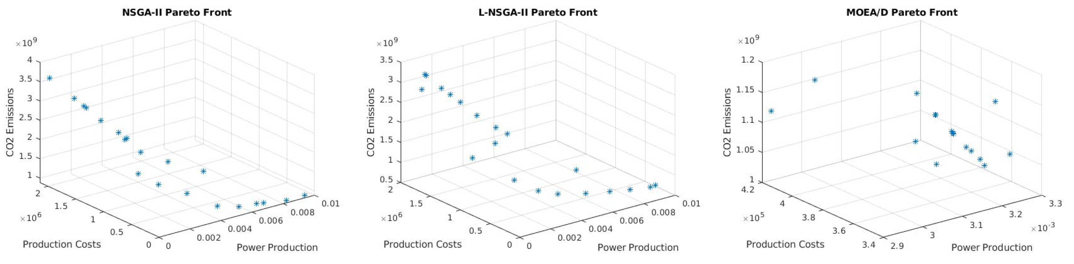
For this metric, NSGA-II and L-NSGA-II obtained larger average values than MOEA/D, leading to conclude that NSGA-II and its variant, L-NSGA-II, both outperformed MOEA/D concerning Hypervolume. Figure 3 displays a sample of the obtained Pareto fronts.
Based on the standard deviations values from both Hypervolume and Spacing (see Table 5), some stability information might be derived. With 14.16 of deviation, the MOEA/D algorithm is presumably the more stable with respect to Spacing measurements, as both NSGA-II and L-NSGA-II present a deviation of 22.68 and 47.67, respectively. In terms of Hypervolume, NSGA-II and L-NSGA-II showed a deviation of 1.95 and 1.99 each, against 2.29 with MOEA/D. Hence, NSGA-II and L-NSGA-II might produce more stable Hypervolume results.
Computational costs are often an issue of interest in the application of metaheuristics. For this matter, Table 6 displays the average execution time of each algorithm on the 25 runs.
The execution times were low in general, and in that context, there are not considerable differences between algorithms to be aware of. Thus, it is suggested to make a decision based solely on the proposed metrics.
The authors of L-NSGA-II suggest that their way to generate the initial population over the traditional method of the original NSGA-II produces more well-distributed solutions. The Spacing metric is then useful to measure such feature. However, for the energy problem stated and solved in this work, it has been shown that (1) NSGA-II and L-NSGA-II provided a similar performance regarding the Spacing metric, i.e., the improved initial population did not lead to better results, and (2) MOEA/D was more suitable to the multi-objetive problem of interest if a better distributed Pareto front is desired.
On the other hand, as this is an application work that might be deployed in a real-world scenario, a competitive solution could be preferred rather than a better distributed one. For this matter, Hypervolume is a more suitable metric. It has been found that (1) NSGA-II and L-NSGA-II presented the same behavior, after the corresponding statistical analysis, and (2) both, NSGA-II and L-NSGA-II, found better solutions than those of MOEA/D.
8. Conclusions and Future Work
Renewable energies play an important role in preserving the quality of the environment. Thus, a power production system was proposed, taking as a case study the state of Oklahoma, composed by solar, wind, and natural gas energies. This system was translated to a Multi-Objective Optimization problem, with three conflicting objective functions: monthly total produced power, monthly production costs, and monthly CO2 emissions. Solar and wind energies highly rely on weather, then a climate model was constructed using previous data from Oklahoma.
Three competitive MOEAs: NSGA-II, L-NSGA-II and MOEA/D were adopted to solve the above mentioned energy production multi-objective problem. The performance assessment was made by using the Spacing and the Hypervolume metrics. After a number of experiments, statistical analysis were carried out in order to validate the findings.
It was found that for this application problem, L-NSGA-II offered no improvement, neither in the distribution of the solutions (its main aim) nor in the quality of the Pareto front. Hence, for this domain problem, the initialization method proposed in L-NSGA-II did not offer an advantage. MOEA/D performed better with respect to the Spacing metric, meaning that it generated more diverse solution sets. Nonetheless, NSGA-II and L-NSGA-II generated more competitive solutions than MOEA/D, as the average Hypervolume value in the former two algorithms was higher than that provided by MOEA/D.
This work encourages new research directions. Concerning the climate model, a more complex data analysis might be convenient, which includes the application of other Machine Learning algorithms to predict solar radiation and wind speed. In order to enrich the power system model, future work also includes the addition of constraints such as generation-demand balance, and to consider the currently installed power capacity characteristics with more detail to increase the model accuracy. A larger metrics ensemble could also be utilized to achieve a more complete characterization of advantages and disadvantages of each algorithm. Finally, metric-based MOEAs will be used to solve the energy production problem.
Author Contributions
Conceptualization, G.-A.V.-H.; methodology, E.M.-M. and G.-A.V.-H.; software, G.-A.V.-H.; data curation, G.-A.V.-H.; investigation, G.-A.V.-H.; formal analysis, G.-A.V.-H. and E.M.-M.; validation, E.M.-M. and E.G.; writting—original draft preparation, G.-A.V.-H., E.M.-M. and E.G.; writing—review and editing, E.G., E.M.-M. and G.-A.V.-H. All authors have read and agreed to the published version of the manuscript.
Funding
The first author acknowledges support from the Mexican National Council of Science and Technology (CONACyT) through a scholarship to pursue graduate studies at University of Veracruz.
Conflicts of Interest
The authors declare no conflict of interest.
Abbreviations
The following abbreviations are used in this manuscript:
| MOEA | Multi-Objective Evolutionary Algorithm |
References
- The Guardian. Available online: https://www.theguardian.com/environment/2018/oct/08/global-warming-must-not-exceed-15c-warns-landmark-un-report (accessed on 15 June 2020).
- US Environmental Protection Agency. Available online: https://www.epa.gov/nutrientpollution/sources-and-solutions-fossil-fuels (accessed on 15 June 2020).
- US Energy Information Administration. Available online: https://www.eia.gov/energyexplained/?page=renewable_home (accessed on 15 June 2020).
- US Department of Energy. Available online: https://www.energy.gov/sites/prod/files/2016/09/f33/OK_Energy%20Sector%20Risk%20Profile.pdf (accessed on 15 June 2020).
- Rodl & Partner. Available online: https://www.roedl.com/insights/erneuerbare-energien/2017-05/renewable-energy-trump-administration (accessed on 15 June 2020).
- AWEA. Available online: http://awea.files.cms-plus.com/FileDownloads/pdfs/Oklahoma.pdf (accessed on 15 June 2020).
- Oklahoma State Government. Available online: https://stateofsuccess.com/industries/energy/solar/ (accessed on 15 June 2020).
- Ganguly, S.; Sahoo, N.C.; Das, D. A novel multi-objective PSO for electrical distribution system planning incorporating distributed generation. Energy Syst. 2010, 1, 291–337. [Google Scholar] [CrossRef]
- Reddy, M.J.; Kumar, D.N. Multiobjective Differential Evolution with Application to Reservoir System Optimization. J. Comput. Civ. Eng. 2007, 21, 136–146. [Google Scholar] [CrossRef]
- Adaryani, M.R.; Karami, A. Artificial bee colony algorithm for solving multi-objective optimal power flow problem. Int. J. Electr. Power Energy Syst. 2013, 53, 219–230. [Google Scholar] [CrossRef]
- Tian, A.Q.; Chu, S.C.; Pan, J.S.; Cui, H.; Zheng, W.M. A Compact Pigeon-Inspired Optimization for Maximum Short-Term Generation Mode in Cascade Hydroelectric Power Station. Sustainability 2020, 12, 767. [Google Scholar] [CrossRef] [Green Version]
- Pan, J.S.; Hu, P.; Chu, S.C. Novel Parallel Heterogeneuous Meta-Heuristic and Its Communication Strategies for the Prediction of Wind Power. Processes 2019, 7, 845. [Google Scholar] [CrossRef] [Green Version]
- Deb, K.; Pratap, A.; Agarwal, S.; Meyarivan, T. A Fast and Elitist Multiobjective Genetic Algorithm: NSGA-II. IEEE Trans. Evol. Comput. 2002, 6, 182–197. [Google Scholar] [CrossRef] [Green Version]
- Wahlroos, M.; Jaaskelainen, J.; Hirvonen, J. Optimisation of an energy system in Finland using NSGA-II evolutionary algorithm. In Proceedings of the 15th International Conference on the European Energy Market (EEM), Lodz, Poland, 27–29 June 2018. [Google Scholar]
- Wang, J.; Zhou, Y. Multi-objective dynamic unit commitment optimization for energy-saving and emission reduction with wind power. In Proceedings of the 5th International Conference on Electric Utility Deregulation and Restructuring and Power Technologies (DRP), Changsha, China, 26–29 November 2015. [Google Scholar]
- Liu, T.; Zhang, D. Multi-Objective Optimal Calculation for Integrated Local Area Energy System Based on NSGA-II Algorithm. In Proceedings of the IEEE International Conference on Energy Internet (ICEI), Nanjing, China, 27–31 May 2019. [Google Scholar]
- Zhou, T.; Sun, W. Optimization of wind-PV hybrid power system based on interactive multi-objective optimization algorithm. In Proceedings of the International Conference on Measurement, Information and Control, Harbin, China, 18–20 May 2012. [Google Scholar]
- Liu, T.; Gao, X.; Wang, L. Multi-objective optimization method using an improved NSGA-II algorithm for oil-gas production process. J. Taiwan Inst. Chem. Eng. 2015, 57, 45–53. [Google Scholar] [CrossRef]
- US OEERE. Available online: https://www.energy.gov/eere/solar/articles/solar-radiation-basics (accessed on 15 June 2020).
- AWEA. Available online: https://www.awea.org/wind-101/basics-of-wind-energy (accessed on 15 June 2020).
- US NRC. Available online: https://www.nrc.gov/reading-rm/basic-ref/glossary/capacity-factor-net.html (accessed on 15 June 2020).
- IRENA. Available online: https://www.irena.org/-/media/Files/IRENA/Agency/Publication/2018/Jan/IRENA_2017_Power_Costs_2018.pdf (accessed on 15 June 2020).
- NASA. Available online: https://climate.nasa.gov/vital-signs/carbon-dioxide/ (accessed on 15 June 2020).
- Moura, P.; de Almeida, A. Multi-Objective Optimization of a Mixed Renewable System with Demand Side Management. Renew. Sustain. Energy Rev. 2010, 14, 1461–1468. [Google Scholar] [CrossRef]
- US Energy Information Administration. Available online: https://www.eia.gov/state/?sid=OK#tabs-4 (accessed on 15 June 2020).
- MESONET. Available online: https://www.mesonet.org/index.php/weather/mesonet_averages_maps#y=average&m=12&p=wspd_mx&d=false (accessed on 15 June 2020).
- Oklahoma, Blue Canyon. Available online: https://bluecanyonwindfarm.com/ (accessed on 15 June 2020).
- Blue Canyon Wind Farm. Available online: https://web.archive.org/web/20061101142429/http://www.horizonwind.com/projects/whatwevedone/bluecanyon/default.aspx (accessed on 15 June 2020).
- Zhang, Q.; Li, H. MOEA/D: A multiobjective evolutionary algorithm based on decomposition. IEEE Trans. Evol. Comput. 2007, 11, 712–731. [Google Scholar] [CrossRef]
- Yen, G.; He, Z. Performance Metrics Ensemble for Multi-Objective Evolutionary Algorithms. IEEE Trans. Evol. Comput. 2013, 18, 131–144. [Google Scholar] [CrossRef]
- Hypervolume Computation. Available online: https://www.mathworks.com/matlabcentral/fileexchange/30785-hypervolume-computation (accessed on 15 June 2020).
- NSGA-II: A Multi-Objective Optimization Algorithm. Available online: https://www.mathworks.com/matlabcentral/fileexchange/10429-nsga-ii-a-multi-objective-optimization-algorithm (accessed on 15 June 2020).
Figure 1.
The proposed power production system for the State of Oklahoma. Each sub-system contributes in the generated power P, the production cost C and the CO2 emissions E.
Figure 1.
The proposed power production system for the State of Oklahoma. Each sub-system contributes in the generated power P, the production cost C and the CO2 emissions E.

Figure 2.
Basic configuration of a wind turbine. The circular surface covered by the three blades is called swept area.
Figure 2.
Basic configuration of a wind turbine. The circular surface covered by the three blades is called swept area.

Figure 3.
Resulting Pareto fronts from NSGA-II (left), L-NSGA-II (center) and MOEA/D (right).


Table 1.
Capacity factors of the three energy sources considered in this work.
| Power Source | Capacity Factor (%) |
|---|---|
| Solar Power | 33 |
| Wind Power | 43 |
| Natural Gas Power | 87 |
Table 2.
Production costs of solar, wind, and natural gas power systems.
| Power Source | Production Cost ($/MWh) |
|---|---|
| Solar Power | 48.2 |
| Wind Power | 33 |
| Natural Gas Power | 15.5 |
Table 3.
CO2 emissions rate of solar, wind and natural gas power systems.
| Power Source | CO2 Emissions Rate (gr/KWh) |
|---|---|
| Solar Power | 49.91 |
| Wind Power | 34.11 |
| Natural Gas Power | 572 |
Table 4.
Boundaries of the decision variables.
| Maximum | 672 h | 672 h | 672 h | 7.07 MW |
| Minimum | 240 h | 240 h | 240 h | 4.88 MW |
Table 5.
Spacing and Hypervolume statistical results, including Average, Standard Deviation and Deviation percentage with respect to the average.
Table 5.
Spacing and Hypervolume statistical results, including Average, Standard Deviation and Deviation percentage with respect to the average.
| Algorithm | Spacing | Hypervolume | ||||
|---|---|---|---|---|---|---|
| Average | Std. Dev. | Deviation % | Average | Std. Dev. | Deviation % | |
| NSGA-II | 22.68 | 1.95 | ||||
| L-NSGA-II | 47.67 | 1.99 | ||||
| MOEA/D | 14.16 | 2.29 | ||||
Table 6.
Average and standard deviation values of execution times of each MOEA measured in seconds.
| NSGA-II | L-NSGA-II | MOEA/D | |
|---|---|---|---|
| Time |
© 2020 by the authors. Licensee MDPI, Basel, Switzerland. This article is an open access article distributed under the terms and conditions of the Creative Commons Attribution (CC BY) license (http://creativecommons.org/licenses/by/4.0/).
Share and Cite
MDPI and ACS Style
Vargas-Hákim, G.-A.; Mezura-Montes, E.; Galván, E. Evolutionary Multi-Objective Energy Production Optimization: An Empirical Comparison. Math. Comput. Appl. 2020, 25, 32. https://doi.org/10.3390/mca25020032
AMA Style
Vargas-Hákim G-A, Mezura-Montes E, Galván E. Evolutionary Multi-Objective Energy Production Optimization: An Empirical Comparison. Mathematical and Computational Applications. 2020; 25(2):32. https://doi.org/10.3390/mca25020032
Chicago/Turabian StyleVargas-Hákim, Gustavo-Adolfo, Efrén Mezura-Montes, and Edgar Galván. 2020. "Evolutionary Multi-Objective Energy Production Optimization: An Empirical Comparison" Mathematical and Computational Applications 25, no. 2: 32. https://doi.org/10.3390/mca25020032