Generalized Confidence Intervals for Zero-Inflated Pareto Distribution

Abstract

This paper considers interval estimations for the mean of Pareto distribution with excess zeros. Three approaches for interval estimation are proposed based on fiducial generalized pivotal quantities (FGPQs), respectively. Simulation studies are performed to assess the performance of the proposed methods, along with three measurements to determine comparisons with competing approaches. The advantages and disadvantages of each method are provided. The methods are illustrated using a real phone call dataset.

1. Introduction

Pareto distribution was introduced by Pareto in 1897 [1]. Since then, it has been widely employed in many applied fields such as meteorology, economics, politics, etc. Confidence intervals (CIs) or approximate CIs for the parameters of a Pareto distribution have been discussed by many authors; Asrabadi derived the unique minimum variance unbiased estimate (UMVUE) for the $100p^{th}$ percentile of a Pareto distribution [2], Chen discussed the exact joint confidence region for the parameters of a Pareto distribution [3], and Wu discussed the interval estimation of a Pareto distribution based on a type II censored sample [4].

In practice, the situation becomes more complicated when the data contain a certain proportion of zeros, as zero values are often neglected by default to avoid complicated calculations. For example, an income in economics and network science data has an excess of zero counts [5]. In such cases, the data include zero values following a zero-inflated Pareto distribution. Previous work for zero-inflated models focused on the Poisson distribution, and the Lognormal distribution indicates that finding the confidence intervals of a zero-inflated Pareto distribution can be performed [6,7,8]. Hasan and Krishnamoorthy proposed confidence intervals for the mean and a percentile based on zero-inflated Lognormal data [9]. Waguespack et al. developed confidence intervals for the mean of a zero-inflated Poisson distribution [10]. However, the interval estimations for the parameters of a zero-inflated Pareto distribution have not been deeply investigated yet.

To the best of our knowledge, there is no published methods to obtain confidence intervals for the mean of a zero-inflated Pareto distribution. In this article, we derive three different approaches to estimate the Fiducial generalized confidence intervals (FGCIs). Since the generalized confidence interval was introduced by Weerahandi [11], it has been widely applied to practical situations where standard solutions do not exist. More details about the FGCIs can be seen in [12,13,14,15].

This article is organized as follows: In Section 2, we develop three different approaches to construct the FGCIs for the mean of the zero-inflated Pareto distribution. In Section 3, we conduct Monte Carlo simulation studies to evaluate coverage probabilities and other measurements of the proposed GCIs. In Section 4, we provide an example with actual data, followed by giving concluding remarks in Section 5.

2. Model and Methods

2.1. Model

Assume that the population of interest contains both zeros and positive observations, such that the probability of having a zero response is $\delta$, where $0<\delta <1$, and that the non-zero observations have a Pareto distribution. Let $X_1,X_2,\dots ,X_n$ be sample from the population, and $n_1$ and $n_0$ be the numbers of non-zero and zero observations, respectively. Without loss of generality, we further assumed that the non-zero observations came first: $X_i>0$ for $i=1,\cdots ,n_1$, and $X_i$ followed a Pareto distribution with shape parameter $\alpha$ and scale parameter c, and $X_i=0$ for $i=n_1+1,\cdots ,n$. Then, $n_0$ followed a binomial distribution with the probability $\delta$, and the probability density function of non-zero observations was:

$$f\left(x\right)=\alpha c^{\alpha }{x}^{-\alpha -1},\alpha >0,c>0,x>c,$$

(1)

and $X_i>0$ for $i=1,\cdots ,n_1$. Then, the mean of the ith population was:

$$\theta =(1-\delta )\frac{\alpha }{\alpha -1}c.$$

(2)

For convenience, let ${\theta }_1=1-\delta$, ${\theta }_2=\frac{\alpha }{\alpha -1}$, and ${\theta }_3=c$; then, $\theta$ could be denoted as $\theta ={\theta }_1\ast {\theta }_2\ast {\theta }_3$.

Based on the properties of exponential distribution, we obtain

$$2n_1\alpha (S-\ln c)\sim {\chi }_2^2,\mathrm{and}2n_1\alpha T\sim {\chi }_{2(n_1-1)}^2,$$

(3)

where $S=\ln X_{\left(1\right)}$ and $T=\left({\sum }_{i=1}^{n_1}\ln X_i-n_1\ln X_{\left(1\right)}\right)/n_1$, S and T are independent.

2.2. Methods

In this section, we proposed three difference methods of constructing confidence intervals for zero-inflated Pareto mean via fiducial inference; fiducial inference was first introduced by Fisher [16], more details can be found in [12,13,17].

Let X be a random vector with a distribution indexed by a parameter $\xi \in \mathrm{\Xi }$, and $\theta =\pi \left(\xi \right)$ be the parameter of interest. Assume that the data-generating mechanism for X could be expressed as:

$$X=G(\xi ,E),$$

(4)

where the distribution of E is known as being independent of any other parameters. Equation (4) can be understood as the equation that was used to generate the data, and it was termed the structural equation. The set-valued function was defined as:

$$Q(x,e)=\{\xi :x=G(\xi ,e\left)\right\},$$

(5)

the function $Q(X,E)$ could be understood as an inverse of the function G. To avoid measurability problems, assume $Q(x,e)$ was a measurable function of u. Notice that the equation $x=G(\xi ,e)$ was satisfied for $\xi$, and e used to generate the observed data x. Assume that the event {$Q(x,e)\ne \varnothing$} happened and the distribution of E had to be conditioned on this event. Then, generalized fiducial distribution of $\xi$ was defined as the conditional distribution:

$$V\left(Q(x,E^{\ast })\right)|\{Q(x,E^{\ast })\ne \varnothing \},$$

(6)

the random variable having the distribution described in (6) is called generalized fiducial quantity (GFQ), which was denoted as $R_{\theta }\left(x\right)$.

In the following, three methods of constructing Fiducial generalized confidence intervals for Pareto distributions were proposed.

2.2.1. Generalized Fiducial Quantities for Parameters of Pareto Distribution

Let $U\sim {\chi }_2^2$ and $V\sim {\chi }_{2(n_1-1)}^2$, and U and V be independent. From (3), we had:

$$U=2n_1\alpha (S-\ln c),V=2n_1\alpha T.$$

For the observed values of s and t, the equation of:

$$(u,v)=(2n_1\alpha (S-\ln c),2n_1\alpha t),$$

had the following unique solution:

$$\alpha =\frac{v}{2n_{1}t},c=exp(s-\frac{u}{v}t).$$

Hence, for given $(s,t)$, the generalized fiducial quantities (GPQs) for $\alpha$ and c were:

$$T_{\alpha }=\frac{V}{2n_{1}t},T_c=exp(s-\frac{U}{V}t),$$

respectively. Therefore, the GPQs of ${\theta }_2$ and ${\theta }_3$ were:

$$T_{{\theta }_2}=\frac{T_{\alpha }}{T_{\alpha }-1}=\frac{V}{V-2n_{1}t},T_{{\theta }_3}=exp(s-\frac{U}{V}t),$$

(7)

respectively.

2.2.2. Proposed $FGC{I}^1$

Because binomial distribution is discrete, it was difficult to obtain the GPQ for $\delta$. Tian derived the GPQs $T_{\delta }^1$ and $T_{\delta }^2$ for $\delta$ based on beta distribution by Tian [7], which was the conjugate prior to binomial distribution,

$$T_{{\delta }_1}\sim beta(n_0+1,n_1),T_{{\delta }_2}\sim beta(n_0,n_1+1),$$

(8)

where $n_0$ and $n_1$ were the numbers of zero and non-zero observations. Then, the two GPQs for population mean $\theta$ were:

$$T_1=(1-T_{\delta }^1)T_{{\theta }_2}{T}_{{\theta }_3},T_2=(1-T_{\delta }^2)T_{{\theta }_2}{T}_{{\theta }_3}.$$

Let $T_1(\gamma /2)$ and $T_2(1-\gamma /2)$ be the $100\gamma /2$th and $100(1-\gamma /2)$th percentiles of $T_1$ and $T_2$, respectively; a $1-\gamma /2$ Fiducial generalized confidence interval (FGCI) was given as:

$$FGC{I}^1:[T_1(\gamma /2),T_2(1-\gamma /2)].$$

In practice, we needed the following Algorithm 1 for $FGC{I}^1$.

Algorithm 1: For a given sample, determine $n_0$ and $n_1$, and calculate observation s and t.

Perform loop: $l=1,2,\cdots ,N$ – Generate $u\sim {\chi }_2^2$ and $v\sim {\chi }_{2n_1-2}^2$, calculate $t_{{\theta }_2}$ and $t_{{\theta }_3}$ by using (7). – Generate $t_{{\delta }_1}$ and $t_{{\delta }_2}$ by (8). – Calculate $t^1=(1-t_{\delta }^1)t_{{\theta }_2}{t}_{{\theta }_3}$, $t^2=(1-t_{\delta }^2)t_{{\theta }_2}{t}_{{\theta }_3}$. Let $T_{i;q}$ denote the $100q$ percentile of ordered $T_i$s ($i=1,2$). Then, $\left[T_{1;\gamma /2},T_{2;1-\gamma /2}\right]$ becomes the $1-\gamma$ GCI of $\theta$.

2.2.3. Proposed $FGC{I}^2$

Let $N_0\sim B(n,\delta )$; binomial distribution was asymptotically normally distributed as the sample size n became large; therefore:

$$Z_w=\frac{N_0-n\delta }{\sqrt{n\delta (1-\delta )}}\sim N(0,1).$$

An alternative approximate GPQ of for $\delta$ by Li [18] was defined as:

$$T_{\delta }^w=\frac{n_0+\frac{Z_w^2}{2}}{n+Z_w^2}-\frac{Z_w}{n+Z_w^2}{\{n_0(1-\frac{n_0}{n})+\frac{Z_w^2}{4}\}}^{\frac{1}{2}},$$

(9)

the distribution of $T_{\delta }^w$ was free of any unknown parameter.

Based on (9), the approximate GPQ for $\theta$ was:

$$T^w=(1-T_{\delta }^w)T_{{\theta }_2}{T}_{{\theta }_3},$$

the approximate $100(1-\gamma )\%$ FGCI for the zero-inflated Pareto mean was denoted as:

$$FGC{I}^2:[{\theta }^w(\gamma /2),{\theta }^w(1-\gamma /2)].$$

The procedure was implemented in the following Algorithm 2.

Algorithm 2: For a given sample, determine $n_0$ and $n_1$, and calculate observation s and t.

Perform loop: $l=1,2,\cdots ,N$ – Generate $u\sim {\chi }_2^2$ and $v\sim {\chi }_{2n_1-2}^2$, calculate $t_{{\theta }_2}$ and $t_{{\theta }_3}$ by using (7). – Generate $t_{\delta }^w$ by (9). – Calculate $t^w=(1-t_{\delta }^w)t_{{\theta }_2}{t}_{{\theta }_3}$. Let $T_q^w$ denote the $100q$ percentile of ordered $t^w$s. Then, $\left[T_{\gamma /2}^w,T_{1-\gamma /2}^w\right]$ becomes the $1-\gamma$ FGCI of $\theta$.

2.2.4. Proposed $FGC{I}^3$

Hannig [13] proposed five ways of finding FGPQ for $\delta$, and simulation studies showed the optimal choice was:

$$T_{\delta }^F\sim \frac{1}{2}beta(n_0,n_1+1)+\frac{1}{2}beta(n_0+1,n_1).$$

(10)

From (10), the approximate GPQ for $\theta$ was:

$$T^F=(1-T_{\delta }^F)T_{{\theta }_2}{T}_{{\theta }_3},$$

and the $100(1-\gamma )\%$ FGCI for the mean of zero-inflated Pareto distribution was denoted as:

$$FGC{I}^3:[{\theta }^F(\gamma /2),{\theta }^F(1-\gamma /2)].$$

Computational details for the FGCI are shown in the following Algorithm 3.

Algorithm 3: For a given sample, determine $n_0$ and $n_1$, and calculate observation s and t.

Perform loop: $l=1,2,\cdots ,N$ – Generate $u\sim {\chi }_2^2$ and $v\sim {\chi }_{2n_1-2}^2$, calculate $t_{{\theta }_2}$ and $t_{{\theta }_3}$ by using (7). – Generate $t_{\delta }^F$ by (10). – Calculate $t^f=(1-t_{\delta }^F)t_{{\theta }_2}{t}_{{\theta }_3}$. Let $T_q^F$ denote the $100q$ percentile of ordered $t^F$s. Then, $\left[T_{\gamma /2}^F,T_{1-\gamma /2}^F\right]$ becomes the $1-\gamma$ FGCI of $\theta$.

3. Simulation Studies

As the proposed methods in the preceding sections were approximate, we introduced three measurements to appraise their validity and accuracies by using the Monte Carlo simulation. The measurements were:

(i) Coverage probabilities (CP): the percentage of the true values that the parameter of interest fell into the confidence intervals we constructed.

(ii) Upper error rate (UER): the ratio of the true values for the parameter of interest that were above the upper limits.

(iii) Lower error rate (LER): the ratio of the true values for the parameter of interest that were below the lower limits.

Our simulation study was conducted with six different proportions of zeros ranging from low to high, combined with different setups of parameters and sample sizes. To estimate the coverage probabilities of the FGCIs for the mean, we generated 2500 samples, each with size n, where each sample contained observations that were zeros and non-zeros, from a $Pareto(\alpha ,c)$ distribution. For each generated sample, we used Algorithms 1–3 with 5000 runs to estimate the 95% CIs. The proportion of 2500 CIs that included the assumed mean was the Monte Carlo estimate of the coverage probability. The estimated coverage probabilities are reported in

Table 1. Coverage probabilities for the mean of a sample with small proportions of zeros.

			${\mathit{FGCI}}^1$			${\mathit{FGCI}}^2$			${\mathit{FGCI}}^3$
$\mathit{\delta }$	n	($\mathit{\alpha },\mathit{c}$)	$\mathit{LW}$	CP	$\mathit{UW}$	$\mathit{LW}$	CP	$\mathit{UW}$	$\mathit{LW}$	CP	$\mathit{UW}$
0.1	10	(2,2)	0.000	0.984	0.016	0.000	0.977	0.023	0.000	0.975	0.025
		(3,2)	0.000	0.980	0.020	0.000	0.971	0.029	0.000	0.964	0.036
		(3,4)	0.000	0.984	0.016	0.000	0.971	0.029	0.000	0.968	0.032
		(10,10)	0.000	0.984	0.016	0.000	0.972	0.028	0.005	0.939	0.056
	30	(2,2)	0.000	0.981	0.019	0.000	0.977	0.023	0.000	0.971	0.029
		(3,2)	0.011	0.979	0.010	0.016	0.970	0.014	0.030	0.947	0.023
		(3,4)	0.018	0.958	0.024	0.027	0.941	0.032	0.047	0.914	0.039
		(10,10)	0.008	0.971	0.021	0.010	0.950	0.040	0.066	0.857	0.077
	100	(2,2)	0.027	0.951	0.022	0.028	0.946	0.026	0.034	0.940	0.026
		(3,2)	0.015	0.956	0.029	0.018	0.949	0.033	0.027	0.933	0.040
		(3,4)	0.020	0.964	0.016	0.026	0.954	0.020	0.039	0.927	0.034
		(10,10)	0.019	0.963	0.018	0.019	0.953	0.028	0.090	0.823	0.087
	2500	(2,2)	0.025	0.948	0.027	0.028	0.946	0.026	0.031	0.939	0.030
		(3,2)	0.021	0.950	0.029	0.022	0.951	0.027	0.033	0.927	0.040
		(3,4)	0.027	0.954	0.019	0.026	0.951	0.023	0.036	0.930	0.034
		(10,10)	0.028	0.951	0.021	0.026	0.953	0.021	0.071	0.855	0.074
0.2	10	(2,2)	0.000	0.976	0.024	0.000	0.969	0.031	0.000	0.968	0.032
		(3,2)	0.000	0.990	0.010	0.000	0.980	0.020	0.008	0.966	0.026
		(3,4)	0.000	0.979	0.021	0.002	0.970	0.028	0.008	0.953	0.039
		(10,10)	0.000	0.991	0.009	0.003	0.974	0.023	0.099	0.842	0.059
	30	(2,2)	0.000	0.976	0.024	0.000	0.967	0.033	0.000	0.963	0.037
		(3,2)	0.000	0.988	0.012	0.000	0.978	0.022	0.007	0.965	0.028
		(3,4)	0.000	0.989	0.011	0.000	0.983	0.017	0.007	0.966	0.027
		(10,10)	0.010	0.978	0.012	0.015	0.959	0.026	0.067	0.860	0.073
	100	(2,2)	0.032	0.948	0.020	0.031	0.949	0.020	0.038	0.936	0.026
		(3,2)	0.023	0.961	0.016	0.028	0.950	0.022	0.048	0.914	0.038
		(3,4)	0.024	0.960	0.016	0.027	0.950	0.023	0.049	0.917	0.034
		(10,10)	0.019	0.964	0.017	0.023	0.955	0.022	0.078	0.855	0.067
	2500	(2,2)	0.026	0.950	0.024	0.027	0.953	0.020	0.031	0.939	0.030
		(3,2)	0.016	0.956	0.028	0.018	0.955	0.027	0.035	0.924	0.041
		(3,4)	0.025	0.955	0.020	0.028	0.952	0.020	0.041	0.926	0.033
		(10,10)	0.022	0.955	0.023	0.021	0.950	0.029	0.081	0.837	0.082

and

Table 2. Coverage probabilities for the mean of a sample with large proportions of zeros.

			${\mathit{FGCI}}^1$			${\mathit{FGCI}}^2$			${\mathit{FGCI}}^3$
$\mathit{\delta }$	n	($\mathit{\alpha },\mathit{c}$)	$\mathit{LW}$	CP	$\mathit{UW}$	$\mathit{LW}$	CP	$\mathit{UW}$	$\mathit{LW}$	CP	$\mathit{UW}$
0.5	10	(2,2)	0.000	0.986	0.014	0.000	0.975	0.025	0.001	0.971	0.028
		(3,2)	0.003	0.991	0.006	0.008	0.977	0.015	0.042	0.933	0.025
		(3,4)	0.006	0.983	0.011	0.008	0.975	0.017	0.038	0.932	0.030
		(10,10)	0.014	0.986	0.000	0.025	0.972	0.003	0.081	0.901	0.018
	30	(2,2)	0.003	0.980	0.017	0.003	0.976	0.021	0.008	0.964	0.028
		(3,2)	0.016	0.971	0.013	0.028	0.955	0.017	0.062	0.899	0.039
		(3,4)	0.014	0.975	0.011	0.025	0.958	0.017	0.065	0.898	0.037
		(10,10)	0.024	0.962	0.014	0.032	0.952	0.016	0.085	0.858	0.057
	100	(2,2)	0.024	0.956	0.020	0.029	0.949	0.022	0.038	0.936	0.026
		(3,2)	0.024	0.962	0.014	0.029	0.950	0.021	0.069	0.890	0.041
		(3,4)	0.022	0.955	0.023	0.025	0.950	0.025	0.070	0.884	0.046
		(10,10)	0.023	0.964	0.013	0.031	0.950	0.019	0.091	0.833	0.076
	2500	(2,2)	0.022	0.953	0.025	0.022	0.954	0.024	0.033	0.931	0.036
		(3,2)	0.028	0.947	0.025	0.026	0.949	0.025	0.058	0.881	0.061
		(3,4)	0.023	0.949	0.028	0.025	0.945	0.030	0.048	0.887	0.065
		(10,10)	0.034	0.945	0.021	0.033	0.949	0.018	0.072	0.852	0.076
0.6	10	(2,2)	0.000	0.989	0.011	0.001	0.979	0.02	0.005	0.96	0.035
		(3,2)	0.012	0.986	0.002	0.019	0.976	0.005	0.054	0.931	0.015
		(3,4)	0.008	0.990	0.002	0.012	0.984	0.004	0.036	0.943	0.021
		(10,10)	0.014	0.986	0.000	0.031	0.969	0.000	0.114	0.874	0.012
	30	(2,2)	0.005	0.976	0.019	0.007	0.973	0.020	0.009	0.967	0.024
		(3,2)	0.023	0.971	0.006	0.030	0.962	0.008	0.073	0.900	0.027
		(3,4)	0.025	0.964	0.011	0.042	0.944	0.014	0.088	0.891	0.021
		(10,10)	0.019	0.973	0.008	0.034	0.952	0.014	0.090	0.851	0.059
	100	(2,2)	0.019	0.959	0.022	0.021	0.955	0.024	0.039	0.925	0.036
		(3,2)	0.024	0.964	0.012	0.032	0.955	0.013	0.066	0.898	0.036
		(3,4)	0.023	0.955	0.022	0.029	0.946	0.025	0.069	0.876	0.055
		(10,10)	0.020	0.961	0.019	0.025	0.946	0.029	0.076	0.844	0.080
	2500	(2,2)	0.020	0.952	0.028	0.020	0.950	0.030	0.036	0.928	0.036
		(3,2)	0.026	0.950	0.024	0.025	0.949	0.026	0.059	0.877	0.064
		(3,4)	0.023	0.950	0.027	0.025	0.947	0.028	0.056	0.890	0.054
		(10,10)	0.023	0.957	0.020	0.029	0.954	0.017	0.075	0.847	0.078

.

We observed from the simulation results that the coverage probabilities were conservative for the proposed methods when the samples were too small in all scenarios. As the sample size became larger, the coverage probabilities for the $FGC{I}^1$ and $FGC{I}^2$ came close to a nominal level, and the coverage probabilities for the $FGC{I}^2$ converged to a nominal level much faster than $FGC{I}^1$. For $FGC{I}^3$, we could see that the coverage probabilities were very sensitive to large values of parameters, as the values of parameters became large, the coverage became very liberal. All three methods proposed a return of fairly balanced tail error rates when the sample sizes became larger. We could also see from the results that no matter how the proportion of zeros changed, it did not affect the coverage probabilities much.

It is noteworthy that, in our simulation studies, we simulated a case with a sample size of 37,000 to show that our proposed methods worked properly for the real-data example in Section 4. Furthermore, our simulation results showed that all three methods returned satisfactory outcomes as long as the parameters were small; when the values of parameters became larger, the coverage probabilities for $FGC{I}^3$ became liberal.

In conclusion, since the simulation results showed that our proposed method two returned satisfactory results according to the coverage probabilities for all different scenarios, we recommend the use of method two in real-world problems.

4. Real-Data Example

In this part, we applied our proposed methods in the network science application [5]. Recently, complex network science has become a significant tool in many fields, such as sociology, climate informatics, finance, as well as genetics, among others (see [5] and the references therein).

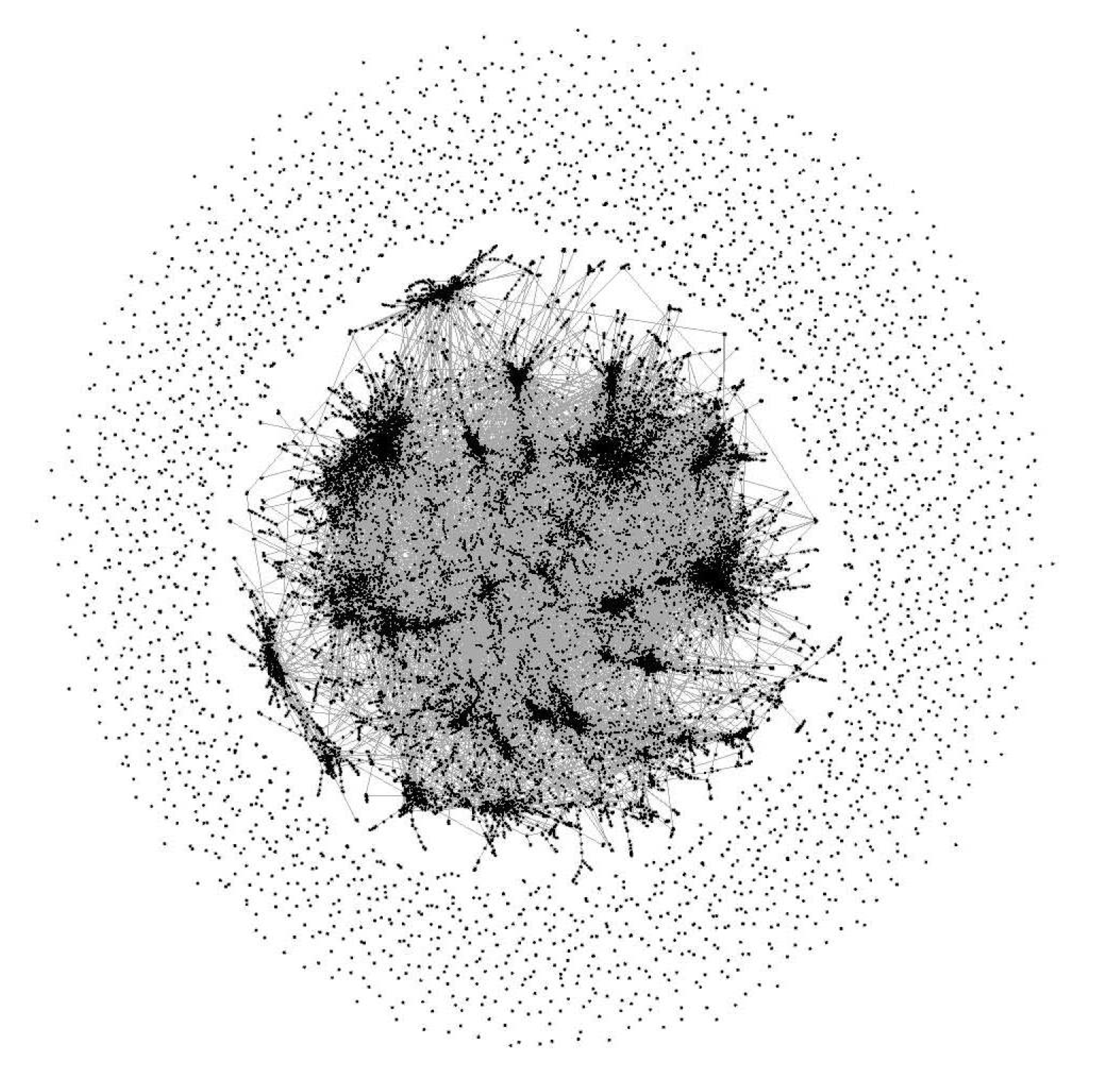
In this example, we considered the phone call network dataset [5], which was directed and contained 36,595 vertexes and 91,826 edges. Figure 1 is an overall visualization of this dataset.

Many of the prototypes in the network science models exhibited a power law phenomenon, namely, the degree (k) distributions of such networks were usually heavy-tailed with the power law distribution [19].

$$p\left(k\right)\propto k^{-\gamma }.$$

(11)

Thus, the Pareto distribution became a natural continuous approximation in such an application, and has been widely investigated in the analysis of the degree distribution of complex networks [20].

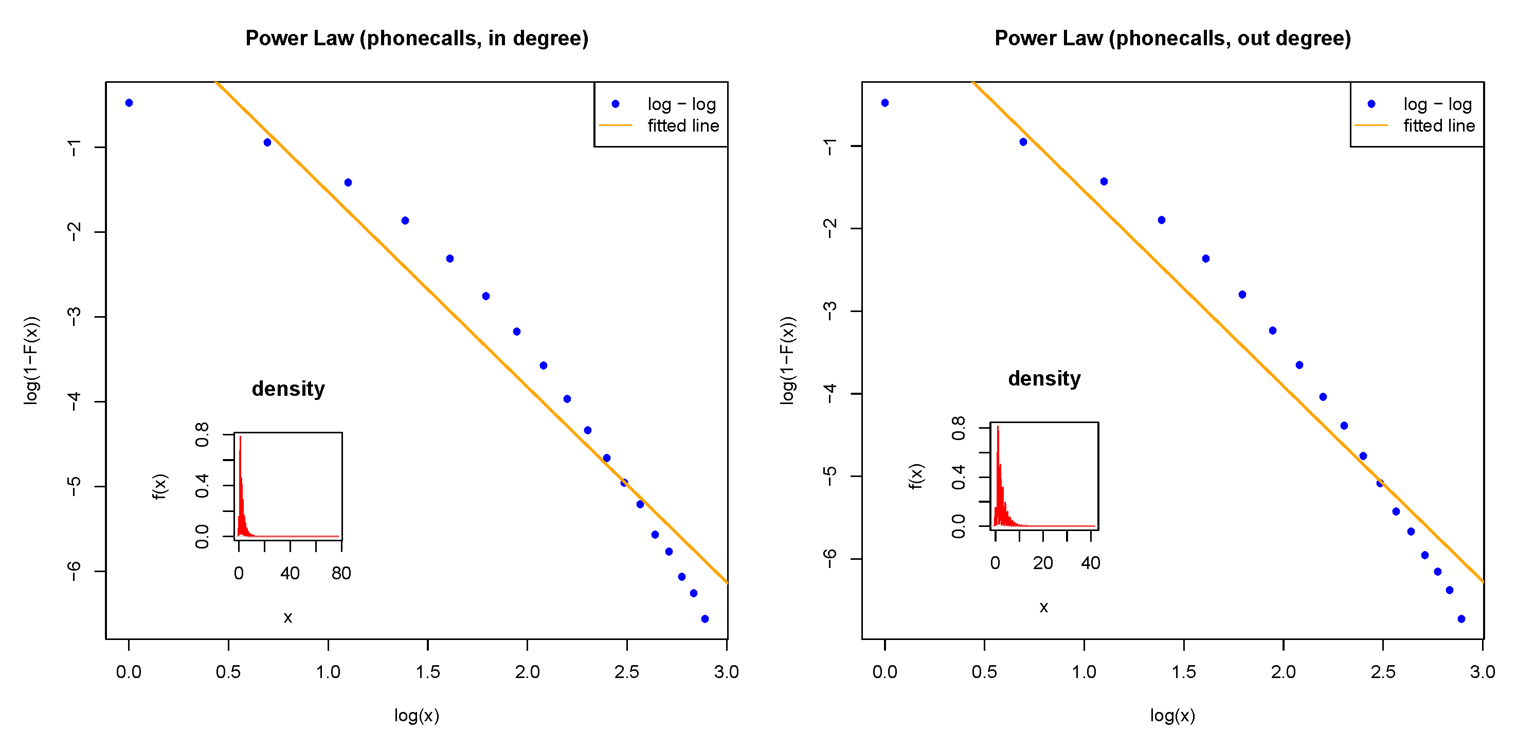
While most degree distributions were focused on the undirected networks, in our example, we focused on the distribution of directed networks. Figure 2 shows the degree distribution for the in-degree (left panel) and out-degree (right panel) in the log–log scale with the survival probability. The straight line results suggested the power law (Pareto) distribution of the data. We also computed the statistic values for both the in-degree and out-degree; the scale and shape parameters for the in-degree were (1.000, 0.109) and the scale and shape parameters for the out-degree were (1.000, 0.110). Both the Pareto probability plots and the statistics values computed showed that the data fit the Pareto distribution well.

For networks without isolated vertexes, all the undirected networks usually had positive degrees. However, on the other hand, not all the in-degrees or the out-degrees, for the directed networks, always had a strictly positive degree. Thus, the zero-inflated Pareto distribution is an ideal tool for modeling the behavior of the degree distribution of the directed networks that follow the power law.

Table 3. Confidence intervals with $2.5\%$ and $97.5\%$ limits for in-degree.

CIs	Lower Limit	Upper Limit
$FGC{I}^1$	3.390	3.603
$FGC{I}^2$	3.390	3.605
$FGC{I}^3$	3.391	3.604

and

Table 4. Confidence intervals with $2.5\%$ and $97.5\%$ limits for out-degree.

CIs	Lower Limit	Upper Limit
$FGC{I}^1$	3.372	3.578
$FGC{I}^2$	3.374	3.575
$FGC{I}^3$	3.376	3.577

present the fitted results for the mean degree distribution (in and out) with our proposed methods. We presented confidence intervals produced by each method in the two tables to show the applicability of our proposed methods. As can be seen from the tables, all of them had consistent results. However, as we mentioned in the simulation analysis, since method two had consistent coverage probabilities for all different scenarios, we recommend the use of the result produced by method two instead of the other results.

5. Conclusions

In this paper, we proposed three approaches to construct the Fiducial generalized confidence intervals for the mean of the zero-inflated Pareto distribution. Detailed computational algorithms were provided and we also conducted an extensive Monte Carlo simulation on various cases to compare the proposed methods. The results showed that the proposed methods were very satisfactory according to the coverage probabilities in simulation studies. Furthermore, we applied our approaches to a real dataset with the application in network science, and they also provided reasonable results for application in real-life situations. What might be needed in future work is to find the confidence intervals for the zero-inflated generalized Pareto distribution.

References

- Pareto, V. Cours d’éConomie Politique; Rouge: Lausanne, Switzerland, 1892. [Google Scholar]
- Asrabadi, B.R. Estimation in the pareto distribution. Metrika 1990, 37, 199–205. [Google Scholar] [CrossRef]
- Chen, Z. Joint confidence region for the parameters of pareto distribution. Metrika 1996, 44, 191–197. [Google Scholar] [CrossRef]
- Wu, S. Interval estimation for a Pareto distribution based on a doubly type II censored sample. Comput. Stat. Data Anal. 2008, 52, 3779–3788. [Google Scholar] [CrossRef]
- Barabasi, A.L.; Posfai, M. Network Science; Cambridge University Press: Cambridge, UK, 2016. [Google Scholar]
- Lambert, D. Zero-inflated poisson regression, with an application to defects in manufacturing. Technometrics 1992, 34, 1–14. [Google Scholar] [CrossRef]
- Tian, L. Inferences on the mean of zero-inflated lognormal data: The generalized variable approach. Stat. Med. 2010, 24, 3223–3232. [Google Scholar] [CrossRef] [PubMed]
- Zhang, Q.; Xu, J.; Zhao, J.; Liang, H.; Li, X. Simultaneous confidence intervals for ratios of means of zero-inflated log-normal populations. J. Stat. Comput. Simul. 2021, 1–20. [Google Scholar] [CrossRef]
- Hasan, M.S.; Krishnamoorthy, K. Confidence intervals for the mean and a percentile based on zero-inflated lognormal data. J. Stat. Simul. Comput. 2018, 88, 1499–1514. [Google Scholar] [CrossRef]
- Waguespack, D.; Krishnamoorthy, K.; Lee, M. Tests and confidence intervals for the mean of a zero-inflated poisson distribution. Am. J. Math. Manag. Sci. 2020, 39, 383–390. [Google Scholar] [CrossRef]
- Weerahandi, S. Generalized confidence intervals. Publ. Am. Stat. Assoc. 1993, 88, 899–905. [Google Scholar] [CrossRef]
- Hannig, J.; Iyer, H.; Patterson, P. Fiducial generalized confidence intervals. Publ. Am. Stat. Assoc. 2006, 101, 254–269. [Google Scholar] [CrossRef]
- Hannig, J. On generalized fiducial inference. Stat. Sin. 2009, 19, 491–544. [Google Scholar]
- Krishnamoorthy, K.; Mathew, T. Inferences on the means of lognormal distributions using generalized p-values and generalized confidence intervals. J. Stat. Plan. Inference 2003, 115, 103–121. [Google Scholar] [CrossRef]
- Tian, L.; Cappelleri, J.C. A new approach for interval estimation and hypothesis testing of a certain intraclass correlation coefficient: The generalized variable method. Stat. Med. 2004, 23, 2125–2135. [Google Scholar] [CrossRef] [PubMed]
- Fisher, R.A. Inverse probability. Math. Proc. Camb. Philos. Soc. 1930, 26, 528–535. [Google Scholar] [CrossRef]
- Li, X.; Su, H.; Liang, H. Fiducial generalized p-values for testing zero-variance components in linear mixed-effects models. Sci. China Math. 2018, 61, 1303–1318. [Google Scholar] [CrossRef]
- Li, X.; Zhou, X.; Tian, L. Interval estimation for the mean of lognormal data with excess zeros. Stat. Probab. Lett. 2013, 83, 2447–2453. [Google Scholar] [CrossRef]
- Clauset, A.; Shalizi, C.R.; Newman, M.E.J. Power-law distributions in empirical data. SIAM Rev. 2009, 51, 661–703. [Google Scholar] [CrossRef] [Green Version]
- Newman, M.E.J. Power laws, pareto distributions and zipf’s law. Contemp. Phys. 2004, 46, 323–351. [Google Scholar] [CrossRef] [Green Version]
Figure 1.
Phone call network dataset.
Figure 2.
Pareto distribution in the log–log scale with the survival probability.