How to Explain the Cross-Section of Equity Returns through Common Principal Components

Abstract

In this paper, we propose a procedure to obtain and test multifactor models based on statistical and financial factors. A major issue in the factor literature is to select the factors included in the model, as well as the construction of the portfolios. We deal with this matter using a dimensionality reduction technique designed to work with several groups of data called Common Principal Components. A block-bootstrap methodology is developed to assess the validity of the model and the significance of the parameters involved. Data come from Reuters, correspond to nearly 1250 EU companies, and span from October 2009 to October 2019. We also compare our bootstrap-based inferential results with those obtained via classical testing proposals. Methods under assessment are time-series regression and cross-sectional regression. The main findings indicate that the multifactor model proposed improves the Capital Asset Pricing Model with regard to the adjusted-$R^2$ in the time-series regressions. Cross-section regression results reveal that Market and a factor related to Momentum and mean of stocks’ returns have positive risk premia for the analyzed period. Finally, we also observe that tests based on block-bootstrap statistics are more conservative with the null than classical procedures.

1. Introduction

Traditionally, finance theory has relied upon the risk-return relationship, i.e., the higher the risk (usually measured through the standard deviation of returns), the higher the return. This concept is at the core of the Capital Asset Pricing Model (CAPM) (see Sharpe [1], Lintner [2], Mossin [3]), where the expected profitability of the i-th stock, $E\left(R_i\right)$, is represented as follows:

$$E\left(R_i\right)=r_f+{\beta }_i(E\left(r_m\right)-r_f),$$

where $r_f$ is the risk-free rate, $E\left(r_m\right)-r_f$ is the Market Risk Premium, and ${\beta }_i$ the sensitivity of expected excess asset’s return associated with the i-th asset.

However, several authors have reported some breaches in this theory. For example, less volatile stocks seem to have higher returns (see Frazzini and Pedersen [4]), while Lintner [2] and Miller and Scholes [5] obtained certain inconsistencies when testing the model with NYSE stocks. Academia has pointed to the existence of several other factors that, beyond volatility, affect the returns of assets (basically, investors obtain a reward for bearing risks different from volatility). Some of these factors, relying on financial measures, are already considered as classical and have been tested in different Markets; see Fama and French [6]. Other factors, that incorporate macro or industry-related measures, such as Interest Rates levels (Viale et al. [7]), or Oil price (Ramos et al. [8]), have been less studied or remain undiscovered. Some researchers, like Elyasiani et al. [9], Lemperiere et al. [10], have focused on higher order statistical moments of returns and, recently, more sophisticated models are built by combining such measures with others involving psychological factors, like Momentum; see Carhart [11]. Momentum, specifically, has won a place by itself among the main factors to be considered in the asset pricing literature and has been tested even in Emerging Markets (see, for example, Misra and Mohapatra [12]). What appears to be clear is that multifactor models should explain the behavior of assets’ returns better than CAPM. However, the number of proposed factors has increased dramatically in recent years. For example, Harvey et al. [13] catalogue 316 factors and note that there are additional ones that do not make it to their final list. Typically, these models take the form of the following equation:

$$E\left(R_i\right)={\alpha }_i+{\beta }_i^{\prime }\lambda .$$

The expected return for the i-th portfolio is linearly related to a set of factors $\lambda$. Usually this set includes CAPM’s Market factor and other additional factors as independent variables. New debates arise today regarding which factors should be included in asset pricing models (see Fama and French [14] and Barillas and Shanken [15] on the methodology to choose among different models and factors and Fama and French [16] regarding the redundancy of the value factor), whether certain factors are not working anymore and what are the main characteristics of extreme performers, equities that experienced extreme return levels during a specific period (for instance, see the work of Heerden and Rensburg [17], where they first choose among different factors and then apply a logistic regression to select shares and build portfolios).

When studying these multifactor models, two main difficulties may appear. First, the procedures to test the significance of the factors rely on the construction of portfolios. We use portfolios instead of stocks since the former have more stable characteristics and are less prone to missing data than the latter and because the errors of $\alpha$ and $\beta$ are higher for individual stocks as their volatility is higher. However, the question on which factors to select in order to build the portfolios remains unanswered. Firstly, there is an issue of dimensionality: on one hand, as we increase the number of portfolios to account for the various factors, the number of companies per portfolio decreases and this could be relevant for analysis of Markets not as developed as the U.S. or the Euro-Zone; on the other hand, there might also be a loss in efficiency in using too few portfolios as the model could fail to explain the cross-section of individual assets. Secondly, as Feng et al. [18] suggest, selecting a few portfolios based on some characteristics could bias the results in favor of these factors. In this paper, we propose to build the portfolios using Common Principal Components (CPC), a multivariate technique developed by Flury [19]. Unlike other dimensionality reduction techniques, specifically the classical principal components that it extends, CPC was designed to be applied when the available information is organized in more than one dataset. In our case, we have several factors measured along a time period for a large group of companies. The idea is to search for a common set of orthogonal axes that capture a high percentage of the variability of the factors observed in all the companies. Using CPC, we respect the individual behavior of each company, which constitutes a group on its own, while keeping a reasonably small number of factors that explain a large part of the variability of the stocks. At the same time, we have made an effort in interpreting each of the CPC factors in terms of the traditional ones.

Second, traditional inferential procedures about multifactor models, like Fama and French [20] and Fama and MacBeth [21], strongly rely on assumptions regarding the data: uncorrelated factors over time, i.i.d. normally distributed errors over time and independent of the factors, etc. When these hypothesis are not fulfilled, classical estimators may be biased. The Bootstrap methodology was developed by Efron [22] as a resampling technique to approximate the distribution of test statistics. In the Asset Pricing literature, Cueto et al. [23] proposed to test test the validity of the model and the significance of the parameters involved through a block-bootstrap procedure that accounts for time dependency. Specifically, we use bootstrap techniques to assess our time-series and cross-sectional regression models by testing, in first place, the hypothesis that the independent terms of the time-series models that explain each of the portfolios returns are jointly zero; thus, the models are able to explain the excess returns. In a second and third stage, significance of the factors for each portfolio are tested, as well as that of the risk premia in the cross-sectional model. The methodological developments in the manuscript end here, since the purpose of these multifactor models in finance is to explain past assets’ behaviors, rather than forecasting.

The resampling procedure described here grows, among others, on that of Chou and Zhou [24], who bootstrap a Wald test for the case where residuals and asset returns are jointly i.i.d and use a block-bootstrap for a Wald-type GMM test in the non-i.i.d case. The block bootstrap was explored by Grané and Veiga [25] in the computation of returns’ unconditional distribution, and huge differences in the estimates of minimum capital risk requirement were reported when using conditional approaches (such as GARCH-type models and stochastic volatility models), particularly for long positions and larger investment horizons.

The objectives of this paper are: (1) to propose a multifactor model based on statistical and financial factors using CPC to reduce its number of dimensions, (2) to develop non-parametric resampling procedures that account for time dependency in order to test model validity and involved parameter significance, and (3) to compare the results obtained via bootstrap-based inferential procedures with those of the classical proposals.

In particular, the financial and statistical factors considered are: Market Capitalization and Total Assets (measures of size), Price to Book ratio (measure of cheapness), Return on Assets and Return on Equity (measures of profitability), Momentum, and four statistical measures (mean, standard deviation, kurtosis, and skewness). The multifactor model with four CPC-factors is able to explain $90\%$ of the variability of the data. The first CPC-factor is a linear combination of mean and Momentum returns; the second and third CPC-factors are linear combinations of skewness and kurtosis returns and finally, the fourth CPC-factor is the standard deviation of the return. Interestingly, none of them include the financial ratios. A possible explanation is that these ratios do not add enough variability compared to statistical factors.

The main findings are that CAPM cannot explain by itself the return of the portfolios as $\beta$ for Market is higher for portfolios with high standard deviation (CPC4) and $\alpha$ is higher (and positive) for portfolios with high Momentum and mean (CPC1). For these time-series models, $R^2$ shows values not greater than 0.55, while despite the wide confirmation of the Market factor in the financial literature, it is not significant in our CAPM cross-section regression analysis, which leads us to conclude the need to control for other factors. When we incorporate additional factors, we notice that Momentum and mean (CPC1-factor), despite being correlated with the Market factor, and standard deviation (CPC4-factor) help explaining the cross-section of European stocks during the period considered. Now, Market $\beta$ stabilize around $0.35$, and CPC1 and CPC4 mainly capture the variability that the Market factor could not explain by itself in CAPM. For these models, we observed a substantial improvement in adjusted-$R^2$, with a median value of 0.671. Apart from the calculation of $\beta$s and $\alpha$s, which seem to be quite robust despite the relaxation of the assumptions of the model, GRS p-value is much higher for the bootstrap (which also occurs in CAPM). Finally, in the cross-section regression, two factors present risk premia different from zero, which are Market and the factor based on mean and Momentum (CPC1-factor). These findings lead us to conclude that the multifactor model based on CPC-factors is a good model with regard to the adjusted-$R^2$, able to explain excess returns, although in the analyzed time period only one of the CPC-factors presents positive risk premia.

The remainder of this paper is organized as follows. Section 2 contains a description of the data and methodology; specifically, in Section 2.1, we present and describe our data, while, in Section 2.2, we explain the methodology used to construct the portfolios and to test the validity the multifactor model, that is, time-series and cross-sectional classical methodologies and the block-bootstrap procedure. Section 3 contains the results of the analysis and the comparison of the application of classical and bootstrap inferential procedures to the data, while the final conclusions are discussed in Section 4.

2. Materials and Methods

2.1. Data and Factors

2.1.1. Data Description

We start with 2393 European companies that were selected from all EU countries. As is usual in the literature on factor models, we excluded Financials as they usually have high leverage ratios, affecting several financial ratios. The database comprises monthly data from Oct-2009 to Oct-2019 and includes prices and several financial ratios, such as Market capitalization, Price to Book and Price to Earnings ratios, number of shares outstanding, Return on Assets and Return on Equity, number of shares traded, and Total Assets. We apply several filters to the Data: first, we delete all companies with less than 30 months of complete data (which leads to 1305 remaining companies); second, we apply a transaction filter, and companies having no transactions for a whole semester were excluded; third, companies with no Market Cap info for more than 2 consecutive years were excluded; finally, companies with non-positive Equity at the end of any year were excluded. We end up with a final set of 1230 companies, after all these filters were passed. Next, monthly returns were computed for all the companies, the Risk Free Rate ($r_f$) and Market ($r_m$) were estimated, respectively, by means of the 2 year German Bond yield and the STOXX 60. Monthly returns were computed as the quotient between the natural logarithms of the market price and the market price in the previous month.

In

Table 1. Summary statistics of the data by year.

Year	Companies	Months	Mean	SD	Min	Median	Max
2009	1230	3	34.70	455.92	0.05	7.61	18,043.85
2010	1230	12	33.76	363.74	0.03	8.15	15,513.50
2011	1230	12	29.23	176.98	0.03	8.57	6515.83
2012	1230	12	26.55	132.78	0.02	7.82	4486.71
2013	1230	12	28.28	116.58	0.03	9.01	3430.00
2014	1230	12	31.64	127.10	0.01	10.95	3800.00
2015	1230	12	35.24	138.22	0.01	12.16	4000.00
2016	1230	12	37.46	166.02	0.01	12.29	5999.00
2017	1230	12	45.42	194.01	0.01	14.95	5999.99
2018	1230	12	47.43	211.38	0.01	14.70	6600.00
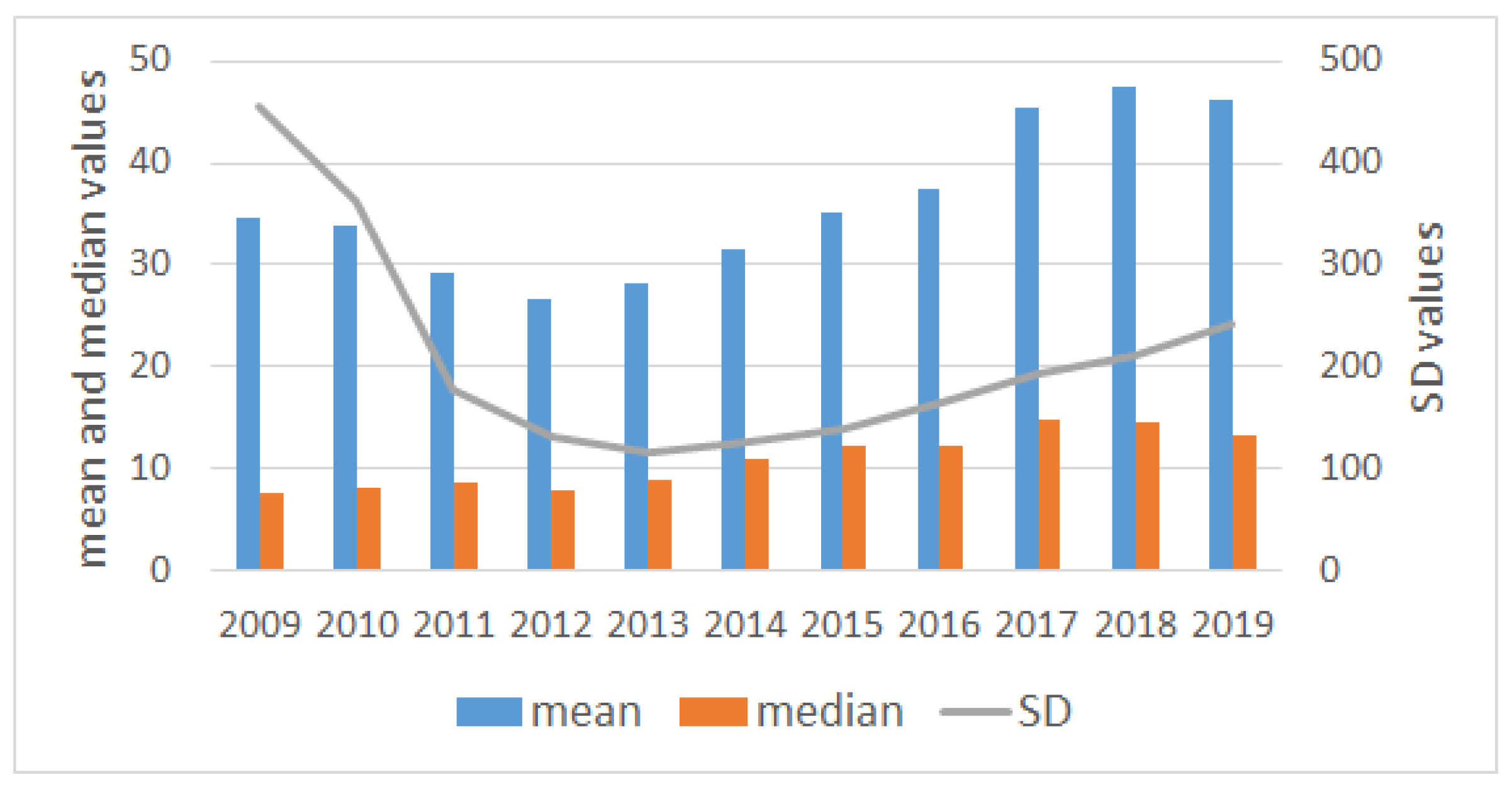
2019	1230	10	46.17	241.41	0.01	13.34	9200.00

, we show some summary statistics by year. In particular, we give information on the number of companies, the number of months, and summary statistics on prices by year. Figure 1 contains a graphical description of the data.

It can be observed that average price experiences a descend until 2012 (from $34.70$ in 2009 to $26.55$ in 2012) and then increases, reaching its maximum value of $47.43$ in 2018. This behavior is related to the 2008 Global Financial Crisis and can be seen more clearly in Figure 1. In terms of standard deviation, we can observe a similar pattern, although the slope in the decrease is more abrupt than for the mean values.

2.1.2. Factors under Study

Cueto et al. [23] introduce three new factors based on statistical measurements on stock prices. Here, we consider such factors calculated on stocks’ returns together with a Momentum variable, which is equal to the 12-month logarithmic return of prices, Market Capitalization and Total Assets (measures of size), Price to Book ratio (measure of cheapness), Return on Assets, and Return on Equity (measures of profitability). For all the financial ratios, we take the value appearing 6 months in advance except for Total Assets, which corresponds to the increment of this measure over the previous 12 months. This way, we incorporate all the factors included in the 5-factor model by Fama and French [16].

Regarding the statistical measures for all the stocks in the sample, we applied a rolling window taking into account the previous 12 observations. These measures are:

• Mean of returns for each year and company:

  $$\overline{x}=\frac{1}{n}\sum _{i=1}^n(x_i-\overline{x}).$$
• Standard Deviation (SD) of returns for each year and company:

  $$s=\sqrt{\frac{1}{n-1}\sum _{i=1}^n{(x_i-\overline{x})}^2}.$$
• Excess Kurtosis (Kurt) of returns for each year and company:

  $$Kurt=\frac{\frac{1}{n}{\sum }_{i=1}^n{(x_i-\overline{x})}^4}{s^4}-3,$$

  which compares the fatness of the distribution tails with respect to those of a normally distributed random variable. Positive values indicate heavier tails than those of the gaussian distribution, whereas negative values indicate thinner tails than the gaussian one.
• Skewness (Skew) of returns for each year and company:

  $$Skew=\frac{\frac{1}{n}{\sum }_{i=1}^n{(x_i-\overline{x})}^3}{s^3},$$

  which measures the asymmetry of the distribution. It takes positive values for positively skewed distributions, that is, when the right tail is longer than the left one, and it takes negative values when the contrary happens. It is roughly zero when both tails are similar (symmetrical distribution).

As can be seen in

Table 2. Correlations among the factors.

	Market	Momentum	Mean	SD	Kurt	Skew	Market Cap	P/B	ROA	ROE	Total Assets
Market	1.000	0.042	0.025	−0.002	−0.001	0.010	−0.006	−0.005	−0.016	−0.005	0.001
Momentum	0.042	1.000	0.959	−0.066	−0.062	0.231	0.008	0.049	0.049	0.199	0.022
Mean	0.025	0.959	1.000	−0.070	−0.062	0.243	0.009	0.054	0.059	0.207	0.023
SD	−0.002	−0.066	−0.070	1.000	0.200	0.036	−0.117	0.010	−0.020	−0.115	−0.009
Kurt	−0.001	−0.062	−0.062	0.200	1.000	0.068	−0.059	0.003	−0.011	−0.029	−0.009
Skew	0.010	0.231	0.243	0.036	0.068	1.000	−0.088	0.008	−0.014	0.012	−0.003
Market Cap	−0.006	0.008	0.009	−0.117	−0.059	−0.088	1.000	0.001	0.081	0.047	0.010
P/B	−0.005	0.049	0.054	0.010	0.003	0.008	0.001	1.000	0.015	0.065	0.008
ROA	−0.016	0.049	0.059	−0.020	−0.011	−0.014	0.081	0.015	1.000	0.187	0.197
ROE	−0.005	0.199	0.207	−0.115	−0.029	0.012	0.047	0.065	0.187	1.000	0.051
Total Assets	0.001	0.022	0.023	−0.009	−0.009	−0.003	0.010	0.008	0.197	0.051	1.000

, Market is positively correlated with Momentum, mean, skewness, and Total Assets, while it is negatively correlated with the remaining factors. This could be useful for investors willing to invest in uncorrelated portfolios (uncorrelated in terms of factors, not assets). Notice further that correlations are mainly low, except for Momentum and mean, which are highly correlated. Such an issue might lead to multicolineality in models considering both factors and, hence, to greater standard errors and larger confidence intervals for the model coefficients.

2.2. Methodology

2.2.1. Common Principal Components

Before analyzing whether certain factors manage to explain the expected return of a set of portfolios, we must first form the portfolios. In order to do so, we use the Common Principal Components technique, introduced by Flury [19], as a generalization of principal components to the case of several groups. The basic assumption in the CPC-model is that the principal component transformation is identical in all the considered groups, while the variances associated with the components may vary between groups. This transformation can be viewed as a rotation yielding variables that are “as uncorrelated as possible” simultaneously in several groups. This distribution-free property justifies the application of the CPC-model to non-normal data. The CPC-model can be also justified from the principle of parsimony, since the number of parameters to be estimated is less than in other usual multivariate methods, which leads to more stable estimations (in the sense of low standard errors). Thus, the underlying idea of CPC-model is to represent in the same common orthogonal axes several groups of individuals/objects (of possibly different sample sizes) for which the same number of variables/measurements have been observed. In our case, it seems reasonable to consider a model in which the same factors occur in different, but related companies. Thus, we can take as variables the ten factors under consideration and groups correspond to the 1230 companies. That is, each group is formed by a particular company and its dataset is composed by the observations of the factors for this particular company along the time period under consideration.

As in classical principal component analysis, the goal is to determine a number of uncorrelated linear combinations of the variables that maximize their variance for each company. In this case, however, despite the fact that the linear combinations will be the same for all companies, the associated variances to each component may change among them, which results in a reduction of the number of parameters to estimate when maximizing the variance explained by the model.

In the setup of the problem, we have f variables $x_1,\dots ,x_f$ (factors) observed on p companies along time periods of size $(n_1,\dots ,n_p)$. Given ${\mathbf{S}}_1,\dots ,{\mathbf{S}}_p$, the variance-covariance matrices of the f variables for each company, we would like to find an orthogonal matrix $\mathbf{U}$ and p diagonal matrices ${\Lambda }_1,\dots ,{\Lambda }_p$ such that:

$${\mathbf{S}}_{\ell }=\mathbf{U}{\Lambda }_{\ell }{\mathbf{U}}^{\prime },\ell =1,\dots ,p,$$

where matrix $\mathbf{U}$ if formed by the common eigenvectors of ${\mathbf{S}}_1,\dots ,{\mathbf{S}}_p$ and diagonal matrix ${\Lambda }_{\ell }$ contains the eigenvalues of each ${\mathbf{S}}_{\ell }$ in descending order.

Note that this model may not exist since, given two positive definite symmetric matrices, their eigenvectors are equal if and only if these matrices fulfill the commutative property. So, in general, matrices ${\mathbf{S}}_{\ell }$ will not have the same eigenvectors, unless they fulfill the commutative property.

Nevertheless, this problem is solved numerically, and the idea is to find a matrix $\mathbf{U}$ and p matrices ${\Lambda }_{\ell }$, such that each $\mathbf{U}{\Lambda }_{\ell }{\mathbf{U}}^{\prime }$ is as similar as possible to ${\mathbf{S}}_{\ell }$. Thus, the CPC-model can be viewed as a rotation yielding variables that are “as uncorrelated as possible” simultaneously in p groups.

To determine how similar they are, Flury and Gaustchi [26] propose a numerical algorithm that minimizes the following discrepancy measure of “simultaneous diagonalizability”:

$$F\left(\mathbf{U}\right)=\prod _{\ell =1}^p{\left[\frac{det\left(\mathrm{diag}\left({\mathbf{U}}^{\prime }{\mathbf{S}}_{\ell }\mathbf{U}\right)\right)}{det\left({\mathbf{U}}^{\prime }{\mathbf{S}}_{\ell }\mathbf{U}\right)}\right]}^{n_{\ell }},$$

(1)

which naturally arises in the context of maximum likelihood estimation in principal component analysis of several groups under the assumption of multivariate normality; see Flury [27].

Proposition 1.

Let ${\mathbf{S}}_1,\dots ,{\mathbf{S}}_p$ be positive definite symmetric matrices of dimension $f\times f$. Then, Expression (1) satisfies that $F\left(\mathbf{U}\right)\ge 1$ and $F\left(\mathbf{U}\right)=1$ if ${\mathbf{S}}_{\ell }=\mathbf{U}{\Lambda }_{\ell }{\mathbf{U}}^{\prime }$, for $\ell =1,\dots ,p$.

The second part of Proposition 1 is straightforward, while the upper bound for $F\left(\mathbf{U}\right)$ follows from Hadamard’s inequality, that we present in Lemma 3 after two preliminary results.

Lemma 1

(Inequality between geometric and arithmetic means). For any $x_1,\dots ,x_n>0$, we have

$${\left(\prod _{i=1}^n{x}_i\right)}^{1/n}\le \frac{1}{n}\sum _{i=1}^n{x}_i.$$

Proof. 

After the convexity of function $\varphi \left(x\right)=-log\left(x\right)$ in ${\mathbb{R}}^{+}$ and Jensen’s inequality,

$$\begin{array}{ccc}\hfill \varphi \left(\frac{1}{n}\sum _{i=1}^n{x}_i\right)& \le & \frac{1}{n}\sum _{i=1}^n\varphi \left(x_i\right)\hfill \\ \hfill -log\left(\frac{1}{n}\sum _{i=1}^n{x}_i\right)& \le & -\frac{1}{n}\sum _{i=1}^{n}log\left(x_i\right)=-log{\left(\prod _{i=1}^n{x}_i\right)}^{1/n}\hfill \\ \hfill {\left(\prod _{i=1}^n{x}_i\right)}^{1/n}& \le & \frac{1}{n}\sum _{i=1}^n{x}_i.\hfill \end{array}$$

   □

Lemma 2.

For any $f\times f$ matrix of correlations $\mathbf{R}$, we have $det\left(\mathbf{R}\right)\le 1$.

Proof. 

Let ${\lambda }_1,\dots ,{\lambda }_f$ be the eigenvalues of $\mathbf{R}$. Applying the inequality between the geometric and arithmetic means given in Lemma 1, we have that

$${(det\left(\mathbf{R}\right))}^{1/f}={\left(\prod _{i=1}^f{\lambda }_i\right)}^{1/f}\le \frac{1}{f}\sum _{i=1}^f{\lambda }_i=\frac{1}{f}\mathrm{tr}\left(\mathbf{R}\right)=1.$$

   □

Lemma 3

(Hadamard’s inequality). For any $f\times f$ positive definite symmetric matrix $\mathbf{S}$, we have $det\left(\mathbf{S}\right)\le {\prod }_{i=1}^f{s}_{ii}$, where $(s_{11},\dots ,s_{ff})=\mathrm{diag}\left(\mathbf{S}\right)$.

Proof. 

Let $\mathbf{S}$ be an $f\times f$ positive definite symmetric matrix and $\mathbf{D}=\mathrm{diag}\left(\mathbf{S}\right)$, then $\mathbf{R}={\mathbf{D}}^{-1/2}\mathbf{S}{\mathbf{D}}^{-1/2}$ is an $f\times f$ matrix of correlations, from where we can obtain $\mathbf{S}$ and compute its determinant as follows:

$$det\left(\mathbf{S}\right)=det\left(\mathbf{D}\right)det\left(\mathbf{R}\right)=\prod _{i=1}^f{s}_{ii}det\left(\mathbf{R}\right)\le \prod _{i=1}^f{s}_{ii},$$

since after Lemma 2, $det\left(\mathbf{R}\right)\le 1.$    □

Preliminary Setup of the Algorithm to Compute the CPC-Model

Flury and Gaustchi [26] propose an algorithm to solve a system of equations that leads to the minimizer of function $F(·)$ in (1) among $f\times f$ orthogonal matrices and for any given $f\times f$ positive definite symmetric matrices ${\mathbf{S}}_1,\dots ,{\mathbf{S}}_p$.

In first place, observe that the denominator in (1) is constant since

$$det\left({\mathbf{U}}^{\prime }{\mathbf{S}}_{\ell }\mathbf{U}\right)=det\left(\mathbf{U}\right)det\left({\mathbf{S}}_{\ell }\right)det\left(\mathbf{U}\right)=det\left({\mathbf{S}}_{\ell }\right).$$

As a consequence, any minimizer of $F\left(\mathbf{U}\right)$ would also be a minimizer of its numerator, which we will denote by $G\left(\mathbf{U}\right)$. Taking logarithms, we have that

$$logG\left(\mathbf{U}\right)=\sum _{\ell =1}^p{n}_{\ell }log(det\left(\mathrm{diag}\left({\mathbf{U}}^{\prime }{\mathbf{S}}_{\ell }\mathbf{U}\right)\right)).$$

The diagonal elements of ${\mathbf{U}}^{\prime }{\mathbf{S}}_{\ell }\mathbf{U}$ are ${\left({\mathbf{U}}^{\prime }{\mathbf{S}}_{\ell }\mathbf{U}\right)}_{ii}={\mathbf{u}}_i^{\prime }{\mathbf{S}}_{\ell }{\mathbf{u}}_i$, where ${\mathbf{u}}_i$ is the i-th column of $\mathbf{U}$. Using this notation, we have that

$$logG\left(\mathbf{U}\right)=\sum _{\ell =1}^p{n}_{\ell }\sum _{i=1}^{f}log\left({\mathbf{u}}_i^{\prime }{\mathbf{S}}_{\ell }{\mathbf{u}}_i\right).$$

Next, the extreme values of $logG\left(\mathbf{U}\right)$ are computed, with the restriction that $\mathbf{U}$ is an orthogonal matrix:

$$\mathsf{\Phi }=logG\left(\mathbf{U}\right)-\sum _{i=1}^f{\mu }_i({\mathbf{u}}_i^{\prime }{\mathbf{u}}_i-1)-\sum _{i=1}^f\sum _{j=1}^f{\mu }_{ij}{\mathbf{u}}_i^{\prime }{\mathbf{u}}_j,$$

(2)

where ${\mu }_i$, ${\mu }_{ij}$, $1\le i,j\le p$, $i\ne j$ are Lagrange multipliers. It can be assumed that ${\mu }_{ij}={\mu }_{ji}$ since ${\mathbf{u}}_i^{\prime }{\mathbf{u}}_j={\mathbf{u}}_j^{\prime }{\mathbf{u}}_i$. Differentiating (2) with respect to ${\mathbf{u}}_k$, we have that

$$\frac{\partial \mathsf{\Phi }}{\partial {\mathbf{u}}_k}=\sum _{\ell =1}^p{n}_{\ell }2{\mathbf{u}}_k^{\prime }{\mathbf{S}}_{\ell }/{\lambda }_{\ell k}-{\mu }_{k}2{\mathbf{u}}_k^{\prime }-\sum _{i=1,i\ne k}^f{\mu }_{ik}{\mathbf{u}}_i^{\prime }=0,$$

where ${\lambda }_{\ell k}$ is the k-th eigenvalue of ${\mathbf{S}}_{\ell }$. Post-multiplying the previous expression by ${\mathbf{u}}_j$, $j\ne k$, we have that:

$$\sum _{\ell =1}^p{n}_{\ell }{\mathbf{u}}_k^{\prime }{\mathbf{S}}_{\ell }{\mathbf{u}}_j/{\lambda }_{\ell k}={\mu }_{jk}.$$

Analogously, differentiating (2) with respect to ${\mathbf{u}}_j$ and post-multiplying the resulting expression by ${\mathbf{u}}_k$, $k\ne j$, one obtains that

$$\sum _{\ell =1}^p{n}_{\ell }{\mathbf{u}}_j^{\prime }{\mathbf{S}}_{\ell }{\mathbf{u}}_k/{\lambda }_{\ell j}={\mu }_{kj}.$$

Subtracting both expressions leads to the following system of equations:

$$\sum _{\ell =1}^p{n}_{\ell }\left(\frac{{\mathbf{u}}_k^{\prime }{\mathbf{S}}_{\ell }{\mathbf{u}}_j}{{\lambda }_{\ell k}}-\frac{{\mathbf{u}}_j^{\prime }{\mathbf{S}}_{\ell }{\mathbf{u}}_k}{{\lambda }_{\ell j}}\right)=0,$$

whose solutions are the columns of matrix $\mathbf{U}$, from which it is possible to obtain matrices ${\Lambda }_{\ell }$. Finally, the system of equations is efficiently solved by means of the aforementioned algorithm of Flury and Gaustchi [26], which is a generalization of the well-known Jacobi method for computing eigenvectors and eigenvalues of a single symmetric matrix.

The CPC algorithm is implemented in the R package multigroup, designed to study multigroup data, where the same set of variables are measured on different groups of individuals. Within this package, we specifically use the function FCPCA to perform the CPC calculation.

2.2.2. Portfolio Construction

In order to build the portfolios in the more rational manner, we first take the proposed financial and statistical measures and standardize them to zero mean and unit variance. We recall that these measures are: Market Capitalization and Total Assets (measures of size), Price to Book ratio (measure of cheapness), Return on Assets and Return on Equity (measures of profitability), Momentum, and the statistical measures already mentioned.

Then, we seek for a common pattern in all companies attending to all measures or factors. Thus, we compute the CPC-model with the aim of obtaining a few uncorrelated components that explain as much as possible the ten measures included in the analysis for all companies. We selected the first four principal components since the average percentage of variability explained by them was $90\%$. Additionally, to check the robustness of the CPC loadings, we estimated them by a bagging procedure [28]. Specifically, we selected groups of 100 companies (without replacement) for which we calculated the CPC-model. After repeating this procedure 5 times, we present the results and compare them with the CPC-model computed with all the data in

Table 3. Loadings computed with all the data vs. loadings computed by bagging.

	Dim 1	Dim 1 (Bagging)	Dim 2	Dim 2 (Bagging)	Dim 3	Dim 3 (Bagging)	Dim 4	Dim 4 (Bagging)
Momentum	70.92	70.77	−0.06	2.15	−4.92	−5.61	2.12	2.32
Mean	70.12	69.82	0.60	2.76	−4.08	−4.62	1.93	2.14
SD	−3.31	−3.78	4.66	4.60	−7.11	−6.04	99.58	99.52
Kurt	−4.40	−7.29	72.27	72.81	−68.46	−67.39	−8.42	−7.81
Skew	4.30	3.02	68.95	68.02	72.26	72.95	2.08	1.27
Market Cap	0.00	0.00	0.00	0.00	0.00	0.00	0.00	−0.01
P/B	0.00	0.01	0.00	0.00	0.00	0.00	0.00	0.00
ROA	0.25	0.32	−0.05	−0.11	−0.08	−0.04	−0.65	−0.85
ROE	2.23	2.33	−0.04	0.08	−0.27	−0.21	−0.69	−1.06
Total Assets	0.02	0.01	−0.03	0.00	−0.04	−0.06	−0.05	−0.10

.

Regarding the bagging results of Table 3, the CPC-loadings changed signs in some iterations and exchanged CPC2 for CPC3 in others (the percentage of variability explained by these two components is very similar–around 22%). Such exchange in some of the components is a well-known problem and is related to the Flury-Gautschi algorithm used to solve (1) [27]. We proceeded to change signs accordingly in order to present consistent results.

Observing the CPC-loadings, we see that the first CPC is a linear combination of mean and Momentum returns, the second and third CPCs are linear combinations of skewness and kurtosis returns and, finally, the fourth CPC is the standard deviation return. In what follows, we call these components CPC1 to CPC4. Interestingly, none of these CPCs include the financial ratios.

Portfolio Setup with the CPC Model

Next, we get the representation of each company in the CPC model (multiplying the loadings by the standardized variables), compute percentiles for each of them and assign to portfolios accordingly, as follows [6].

• Stocks with low CPC1 are included in portfolios 1-b-c-d, while stocks with high CPC1 are included in portfolios 2-b-c-d.
• Stocks with low CPC2 are included in portfolios a-1-c-d, while stocks with high CPC2 are included in portfolios a-2-c-d.
• Stocks with low CPC3 are included in portfolios a-b-1-d, while stocks with high CPC3 are included in portfolios a-b-2-d.
• Stocks with low CPC4 are included in portfolios a-b-c-1, while stocks with high CPC4 are included in portfolios a-b-c-2.

In

Table 4. Description of portfolios.

Portfolio Number	Portfolio Description	Portfolio Composition
		CPC1	CPC2	CPC3	CPC4
1	1-1-1-1	Low	Low	Low	Low
2	1-1-1-2	Low	Low	Low	High
3	1-1-2-1	Low	Low	High	Low
4	1-1-2-2	Low	Low	High	High
5	1-2-1-1	Low	High	Low	Low
6	1-2-1-2	Low	High	Low	High
7	1-2-2-1	Low	High	High	Low
8	1-2-2-2	Low	High	High	High
9	2-1-1-1	High	Low	Low	Low
10	2-1-1-2	High	Low	Low	High
11	2-1-2-1	High	Low	High	Low
12	2-1-2-2	High	Low	High	High
13	2-2-1-1	High	High	Low	Low
14	2-2-1-2	High	High	Low	High
15	2-2-2-1	High	High	High	Low
16	2-2-2-2	High	High	High	High

, we summarize the resulting portfolios, which are updated monthly based on the previous month measurements. For each portfolio, we calculate the average monthly returns. Additionally, each factor is computed as the excess return of the higher portfolio in each category minus the return of the lower portfolio. All returns are calculated for equally-weighted portfolios at $t+1$. Figure 2 contains the cumulative returns of the portfolios.

As we commented before, it is interesting that none of the CPCs include financial measures, which might occur because these ratios do not add enough variability compared to statistical factors. However, in a way, statistical measures could be also capturing some of the financial characteristics of the stocks as we see in

Table 5. Characteristics of portfolios.

Portfolio	Portfolio	Portfolio Composition (Mean Values)
Number	Description	Market Cap	Total Assets	PB	ROA	ROE	MOM	Mean	sd	Kurt	Skew
1	1-1-1-1	4922.44	8816.40	1.94	4.57	8.47	−0.086	−0.008	0.057	2.935	−0.555
2	1-1-1-2	2072.12	6275.54	1.64	1.80	−0.28	−0.233	−0.021	0.116	2.865	−0.580
3	1-1-2-1	4063.73	6734.97	1.88	4.48	7.93	−0.094	−0.009	0.055	2.161	0.025
4	1-1-2-2	1839.13	5504.61	1.56	1.84	−4.27	−0.233	−0.021	0.108	2.079	0.000
5	1-2-1-1	3263.27	6024.39	1.84	4.22	7.74	−0.075	−0.007	0.059	4.308	−0.189
6	1-2-1-2	1044.30	3209.33	1.46	1.37	−14.23	−0.241	−0.022	0.146	4.263	−0.227
7	1-2-2-1	2795.40	4915.16	1.75	4.05	5.53	−0.080	−0.007	0.055	2.961	0.575
8	1-2-2-2	1025.77	3036.45	1.62	1.41	−9.23	−0.208	−0.019	0.118	2.853	0.558
9	2-1-1-1	6655.51	8231.53	2.65	7.33	14.65	0.186	0.017	0.058	2.729	−0.494
10	2-1-1-2	2654.52	4986.17	2.50	5.76	11.55	0.306	0.028	0.106	2.614	−0.440
11	2-1-2-1	6033.27	7107.41	2.52	7.26	14.15	0.172	0.016	0.055	2.089	0.023
12	2-1-2-2	2570.95	4606.20	2.42	5.76	10.76	0.284	0.026	0.099	1.999	0.068
13	2-2-1-1	2946.72	3876.48	2.33	6.85	12.89	0.169	0.016	0.060	4.068	0.222
14	2-2-1-2	1218.32	2307.18	2.29	5.23	10.51	0.369	0.034	0.140	4.121	0.502
15	2-2-2-1	3016.33	3701.31	2.32	7.13	13.15	0.172	0.016	0.056	2.943	0.600
16	2-2-2-2	1031.39	2519.19	2.15	6.31	8.45	0.333	0.031	0.111	2.877	0.672

, which includes average factors for each of the portfolios considered and standard deviation, kurtosis, and skewness of the returns. We notice, for example, that portfolios with high CPC1 present in average higher PB ratio, higher ROA and ROE, lower kurtosis, and positive skew. Portfolios with high CPC4 show in average lower PB ratio, lower ROA and ROE, lower kurtosis, and higher skew.

The best portfolios are those with high mean and Momentum (CPC1), except for portfolio 2-2-1-2, while the three portfolios with the poorest performances are 1-1-2-2, 1-2-2-2, and 1-1-1-2. They share the feature of having low mean and Momentum (CPC1) and high standard deviation (CPC4).

2.2.3. Classical Methodologies

Once we have defined the N portfolios that we are about to analyze, we perform a time-series regression for each of them:

$$R_t^i-r_f={\alpha }_i+{\beta }_i^{\prime }{f}_t+{ϵ}_t^i,t=1,2,\dots ,T.$$

We use the GRS test by Gibbons et al. [29] to assess the ability of a model to explain excess returns. The null hypothesis of this test is $H_0:{\alpha }_1=\dots ={\alpha }_N=0$, and assuming that $ϵ$s are normally distributed, the test statistic is given by:

$$\frac{T-N-K}{N}{[1+{\overline{f}}^{\prime }{\Sigma }_f^{-1}\overline{f}]}^{-1}{\widehat{\alpha }}^{\prime }{\Sigma }^{-1}\widehat{\alpha }\sim F_{N,T-N-K},$$

(3)

where K is the number of factors, ${\Sigma }_f$ is the factors’ covariance matrix, and $\Sigma$ the residual covariance matrix. The purpose of the test, whose statistic takes also into account the sampling error of estimates in ${\beta }_i$, is to determine if the ${\alpha }_i$ are jointly zero assuming that the distribution of returns and factors is multivariate normal. As suggested by Fama [30], the GRS test is against an unspecified alternative, both for portfolios and factors. On the one hand, the model may pass the test for a set of portfolios, but fail for another. On the other hand, we do not specify additional factors that could produce a violation of the model (however, we get some intuition on which factors should be included or excluded from the model by observing the number of portfolios whose coefficients are significantly different from zero).

Then, we run a cross-sectional regression to estimate the vector of risk premia $\lambda$ with the model obtained taking expectations in the time-series regression equation:

$$E(R^i-r_f)={\widehat{\alpha }}_i+{\widehat{\beta }}_i^{\prime }\lambda ,\mathrm{for}i=1,\dots ,N,$$

where the estimates for ${\widehat{\beta }}_i$ are those obtained in the TS regression at the first step. In conclusion $\widehat{\lambda }$ represents the slope coefficients in the cross-sectional regression which is run without intercept, while $\widehat{\alpha }$ are the residuals in the cross-sectional regression. If the estimated $\beta$s are important determinants of average returns, then the risk premium, ${\lambda }_i$, should be statistically significant. We have used the covariance of the residuals of the TS regression to calculate the standard error of ${\lambda }_i$ to take into account the correlation across assets. Additionally, the error terms for ${\lambda }_i$ must include the error of estimating $\beta$[31] for the so-called Shanken correction, although the difference may be very small in practice. Finally, we use t-statistics to test the significance of each of the ${\lambda }_i$.

2.2.4. Resampling Techniques: Bootstrap

As in Reference [23], we follow a block-bootstrapping pairs scheme to preserve the time correlation of the data, and take B bootstrap samples of block size $b=2$ months. We describe briefly the procedure and refer to the original paper for further details.

• Step 1 Estimate benchmark regression models, one for each portfolio. For each portfolio, save $\alpha$, $\beta$, their corresponding t-statistics, residuals, risk factors’ estimates, and GRS statistic.
• Step 2 Produce a set of simulation runs equal for each portfolio in order to preserve returns’ cross-correlations.
• Step 3 Build a new series of $\alpha$-free portfolio returns by using the simulated time indices.
• Step 4 Run the time-series factor model regression on the artificially constructed returns. Calculate $\widehat{\alpha }$, $\widehat{\beta }$ and the corresponding confidence intervals. Next, generate samples of the GRS Statistic, compute different percentiles from the bootstrapped distribution and compare them to the original GRS statistic.
  In this paper, we improve the methodology proposed in our previous work. We have noticed that, given the construction of the GRS statistic, when we face portfolios with heteroskedasticity, the estimation of the variance through the residual covariance matrix may not be appropriate. Thus, we propose a new statistic, $Q\left(\alpha \right)={\widehat{\alpha }}^{\prime }{\Sigma }^{-1}\widehat{\alpha }$, for which we will calculate the covariance matrix of $\alpha$s, $\Sigma$, through a nested bootstrap. Then, a new step appears:
• Step 5 Run the time-series factor model regression on the artificially constructed returns. Calculate $\widehat{\alpha }$, $\widehat{\beta }$ and the corresponding confidence intervals. Finally, generate bootstrap samples of the $Q\left(\alpha \right)$ statistic that makes use of the covariance matrix of the $\alpha$s which is approximated by means of a nested bootstrap and compare the bootstrapped statistics with the original $Q\left(\alpha \right)$ statistic.
  Concerning cross-sectional regression, we use $\beta$s and average returns from each bootstrapped sample to determine the significance of the risk premia estimates ($\lambda$s). Given that $\beta$s are estimated, the estimates of the $\lambda$s might present substantial bias and we use a reverse bootstrap percentile interval to determine the significance of the factors. To be consistent, we also present this type of bootstrap interval for all the estimated parameters.

As this is a computer-intensive method, we implemented the previous procedure in R by using the R-packages doParallel and foreach, designed to do multi-core calculations. The main reason for using the foreach package is that it supports parallel execution, that is, repeated operations can be executed on multiple cores of the computer or on multiple nodes of a cluster, thus reducing the execution time.

3. Results

3.1. Time-Series Regressions

In this section, we present the results for the time-series regression of two models. The first one is the CAPM model and the second one is a multifactor model including Market and four factors determined by CPC1 to CPC4. The dependent variables are the returns of the 16 portfolios.

3.1.1. Model 1: CAPM

When we analyze a 1-factor model, only taking into consideration the Market factor, we notice that the p-value of the GRS statistic is $1.93\%$, thus rejecting that all $\alpha$s are jointly zero at $5\%$ significance level. This could be an indication that other factors are missing because the portfolios are sorted to have greater cross-section differences, but, given that this is a well studied factor, we would like to understand if this rejection may be due to an anomalous period of time and/or to a breach in certain assumptions of the model.

First, we split the 108 months in two periods: from 1 to 80 (first subperiod) and from 30 to 108 (second subperiod), both with approximately the same number of months. We find that the GRS p-value for the first subperiod is $3.43\%$, while the p-value for the second subperiod is $0.24\%$. This could indicate that the CAPM may have not behaved correctly during the second period, while global Central Banks have been injecting huge amounts of liquidity in the system.

Additionally, in order to confirm if the OLS hypotheses are fulfilled (normality, homoscedasticity and independence), we performed several analysis following Soumaré et al. [32]. The results are presented in

Table 6. Metrics for CAPM with different time periods.

	Statistics (p-Value)			Number of Portfolios
	GRS	GRS Boot.	$\mathit{Q}\left(\mathbf{\alpha }\right)$	Non-Normal	Heteros.	Autocorr.
Whole period	$2.024$ ($1.93\%$)	$2.024$ ($17.4\%$)	$42.57$ ($29.5\%$)	6	4	5
Months 1–80	$1.924$ ($3.43\%$)	$1.924$ ($8.2\%$)	$38.62$ ($27.5\%$)	3	5	4
Months 30–108	$2.736$ ($0.24\%$)	$2.736$ ($17.8\%$)	$61.35$ ($30.6\%$)	3	1	8

, where we show the different statistics analyzed with their p-values in parentheses and the number of portfolios for which we reject the null at a $5\%$ significance level for the different tests.

A Shapiro-Wilk test was run on each set of residuals, suggesting that, in general, if we consider both subperiods individually, the residuals of the time-series regression are normally distributed. This changes when we consider the whole period, where 6 portfolios have a p-value lower than $5\%$ in the test. Generally, these are portfolios with high mean and Momentum (CPC1) and low standard deviation (CPC4).

Additionally, we performed a Breusch-Pagan test on the residuals of the regressions, showing that the homoscedasticity assumption is violated for portfolios 9, 10, 11 and 13 (all of them share the characteristic of having a high mean and Momentum (CPC1) and, generally, present low levels of the remaining CPCs). Interestingly, during the second subperiod, we reject the homocedasticity only for portfolio 16.

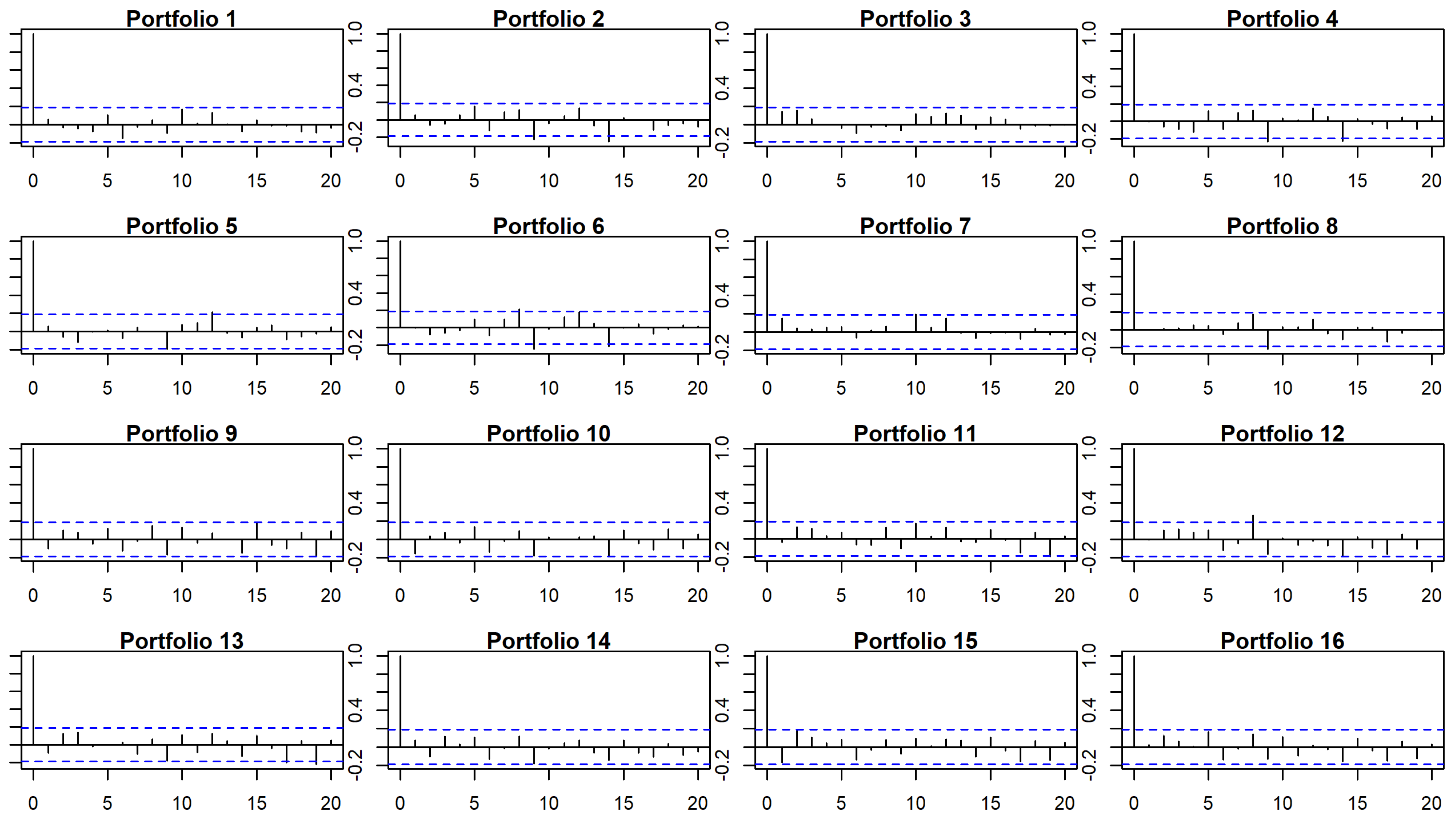
In Figure 3, we show the autocorrelation charts for errors in time-series regression for CAPM for the whole period. The charts indicate that residuals are especially correlated for lags equal to or higher than 9. The Durbin-Watson test also suggests that errors might be autocorrelated for 5 portfolios for lag equal 9 when considering the whole period (generally, those with low mean and Momentum (CPC1) and high standard deviation (CPC4)), 4 for the first subperiod and 8 for the second one (p-values lower than $5\%$).

These three facts suggest that the bootstrap procedure developed in Reference [23] might be useful to approximate the distribution of the GRS statistic. Applying this procedure (see Table 6), we obtained a bootstrap p-value of $17.4\%$ for the whole period, so we cannot reject that the $\alpha$s are jointly zero. Something similar happens when we consider the first subperiod (GRS p-value of $8.2\%$) and the second subperiod (GRS p-value of $17.8\%$). However, we do not feel comfortable with the results as the p-values of the Bootstrap are far away from the p-values of the traditional methodology; remember that the GRS test estimates $\Sigma$ through the residual covariance matrix. We suspect that the existence of heteroscedasticity in some of the portfolios could make this estimation inaccurate. Thus, we propose a new statistic, $Q\left(\alpha \right)={\widehat{\alpha }}^{\prime }{\Sigma }^{-1}\widehat{\alpha }$, for which we will calculate the covariance matrix of $\alpha$s, $\Sigma$, through a nested bootstrap. The results obtained with the $Q\left(\alpha \right)$ statistic reinforce the conclusions reached with the GRS bootstrap, since the p-values of this new statistic are even higher than those of the former (between 1.6 and 3.3 times). Thus, we do not reject that the $\alpha$s are jointly zero at a $5\%$ significance level.

In

Table 7. Results for Time-Series estimation of CAPM.

	Estimates		t-Statistics		Bootstrap CI $(2.5\%,97.5\%)$
Portfolio	$\mathbf{\alpha }$	Market	$\mathbf{\alpha }$	Market	$\mathbf{\alpha }$	Market	${\mathit{R}}^{\mathbf{2}}$
1	−0.001	0.685	−0.546	10.856	−0.007, 0.002	0.533, 0.845	0.526
2	−0.003	0.954	−0.695	9.109	−0.013, 0.002	0.746, 1.161	0.439
3	−0.004	0.543	−1.068	4.982	−0.016, −0.002	0.324, 0.736	0.190
4	−0.005	0.946	−1.235	8.853	−0.018, −0.002	0.722, 1.172	0.425
5	0.000	0.485	−0.041	7.141	−0.006, 0.004	0.317, 0.649	0.325
6	−0.003	0.823	−0.680	7.380	−0.014, 0.002	0.604, 1.024	0.339
7	−0.002	0.542	−0.905	7.948	−0.010, 0.001	0.389, 0.716	0.373
8	−0.004	0.831	−1.032	7.702	−0.016, −0.001	0.577, 1.078	0.359
9	0.004	0.632	1.655	9.304	0.003, 0.012	0.432, 0.840	0.450
10	0.005	0.865	1.398	8.898	0.003, 0.016	0.622, 1.097	0.428
11	0.004	0.619	1.647	8.967	0.003, 0.013	0.398, 0.827	0.431
12	0.003	0.852	0.960	8.613	0.000, 0.014	0.602, 1.112	0.412
13	0.004	0.532	1.936	8.128	0.004, 0.013	0.362, 0.725	0.384
14	0.000	0.657	0.128	6.932	−0.006, 0.008	0.472, 0.847	0.312
15	0.006	0.454	2.300	6.467	0.007, 0.015	0.264, 0.628	0.283
16	0.005	0.729	1.459	7.672	0.003, 0.016	0.500, 0.991	0.357

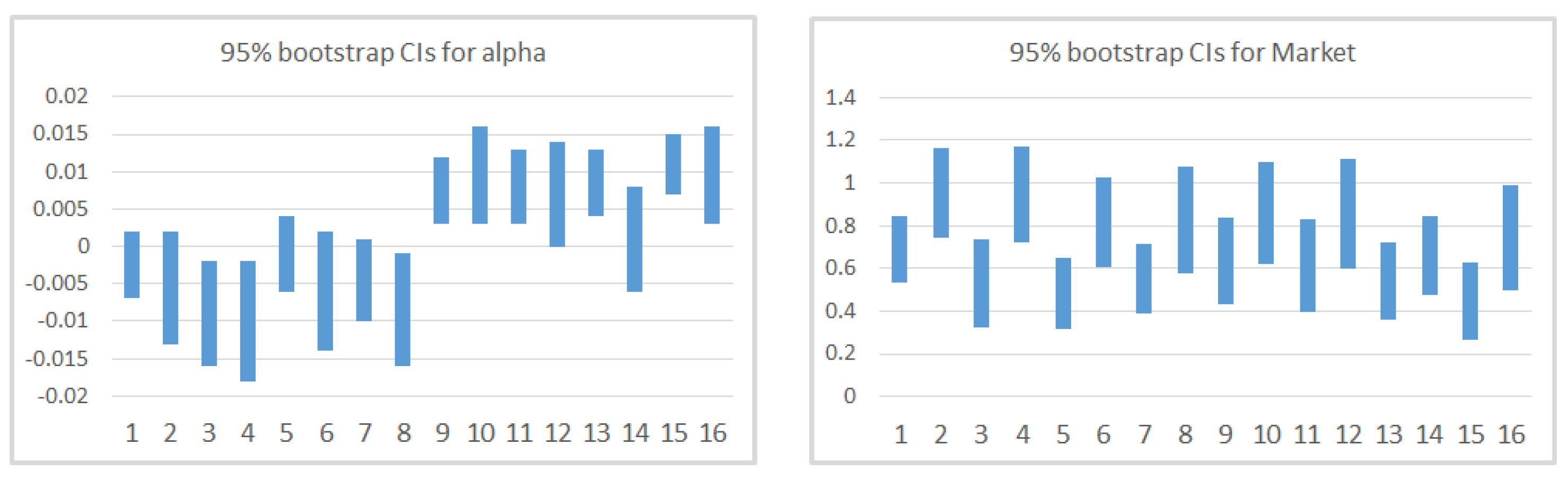
Notes. GRS: 2.024, p-value: 0.0193, p-value Boot.: 0.174, p-value Q($\alpha$): 0.295.

, we present the results for the classical and the bootstrap methodologies for Model 1. Columns “Estimates” contain the estimates for $\alpha$ and $\beta$ for Market. The classical t-statistics for these estimates are in columns 4 and 5. Columns 6 and 7 correspond to the basic bootstrap confidence intervals and $R^2$ is reported in the final column. A graphical comparison is given in Figure 4. Regarding the estimates of the model, we find that the coefficient for Market is always positive and statistically significant for classical methodology and for the resampling technique. The estimate varies between $0.95$ and $0.45$, but it is, in general, higher for portfolios with high standard deviation (CPC4). This confirms the traditional relationship between expected return and $\beta$ explained in the CAPM. However, as we will see later and as different studies have suggested, this relationship does not hold once we include new factors and review the cross-section regression. The coefficients of determination indicate that this model explains between $19.0\%$ and $52.6\%$ of the variability of portfolios’ returns. Moreover, under the classical inferential techniques, we find that $\alpha$ is not statistically significant (except for portfolio 15) which is positive for portfolios with high mean and Momentum (CPC1) and negative otherwise. The resampling technique finds more portfolios where $\alpha$ is statistically significant. As we have already discussed, the GRS test rejects, at a $5\%$ significance level, that all pricing errors are equal to zero which might indicate that other factors are missing.

3.1.2. Model 2: Market and Factors CPC1 to CPC4

When we analyze the 5-factor model, we notice that the p-value of the GRS statistic is $0.90\%$, lower than in the previous model and also rejecting, at a $5\%$ significance level, that all $\alpha$s are jointly zero. This could indicate that the model does not reflect correctly the variability of the returns of the portfolios.

As before, we split the 108 months in two periods: from 1 to 80 (first subperiod) and from 30 to 108 (second subperiod). We find that the GRS p-value for the first subperiod is $5.19\%$, while the p-value for the second subperiod is $0.38\%$. This could indicate that this model has not behaved correctly during the second subperiod, as we discussed for the previous model. Results for GRS p-values (both for classical and resampling methodology), $Q\left(\alpha \right)$ p-value and normality, heteroscedasticity and autocorrelation tests are presented in

Table 8. Metrics for 5-factors model with different time periods.

	Statistics (p-Value)			Number of Portfolios
	GRS	GRS Boot.	$\mathit{Q}\left(\mathbf{\alpha }\right)$	Non-Normal	Heteros.	Autocorr.
Whole period	$2.242$ ($0.90\%$)	$2.242$ ($17.1\%$)	$56.59$ ($22.6\%$)	10	1	12
Months 1–80	$1.806$ ($5.19\%$)	$1.806$ ($22\%$)	$44.92$ ($32.8\%$)	1	1	7
Months 30–108	$2.625$ ($0.38\%$)	$2.625$ ($13\%$)	$56.19$ ($27.8\%$)	8	1	7

.

For this second model, the Shapiro-Wilk test run on each set of residuals suggests that the number of non-normal portfolios is higher than in the previous model. In fact, when we consider the whole period, 10 portfolios have a p-value lower than $5\%$ in the test. If we consider both subperiods individually, we can only reject the null for one portfolio in subperiod 1 (portfolio 5), while there are 8 portfolios with this same characteristic in subperiod 2.

We also ran a Breusch-Pagan test on the residuals of the regressions, showing that the homoscedasticity assumption is violated for portfolio 11 during subperiod 1 and portfolio 14 during the second subperiod and the whole period. In this model, the heteroscedasticity problem seems to be (at least, partially) solved.

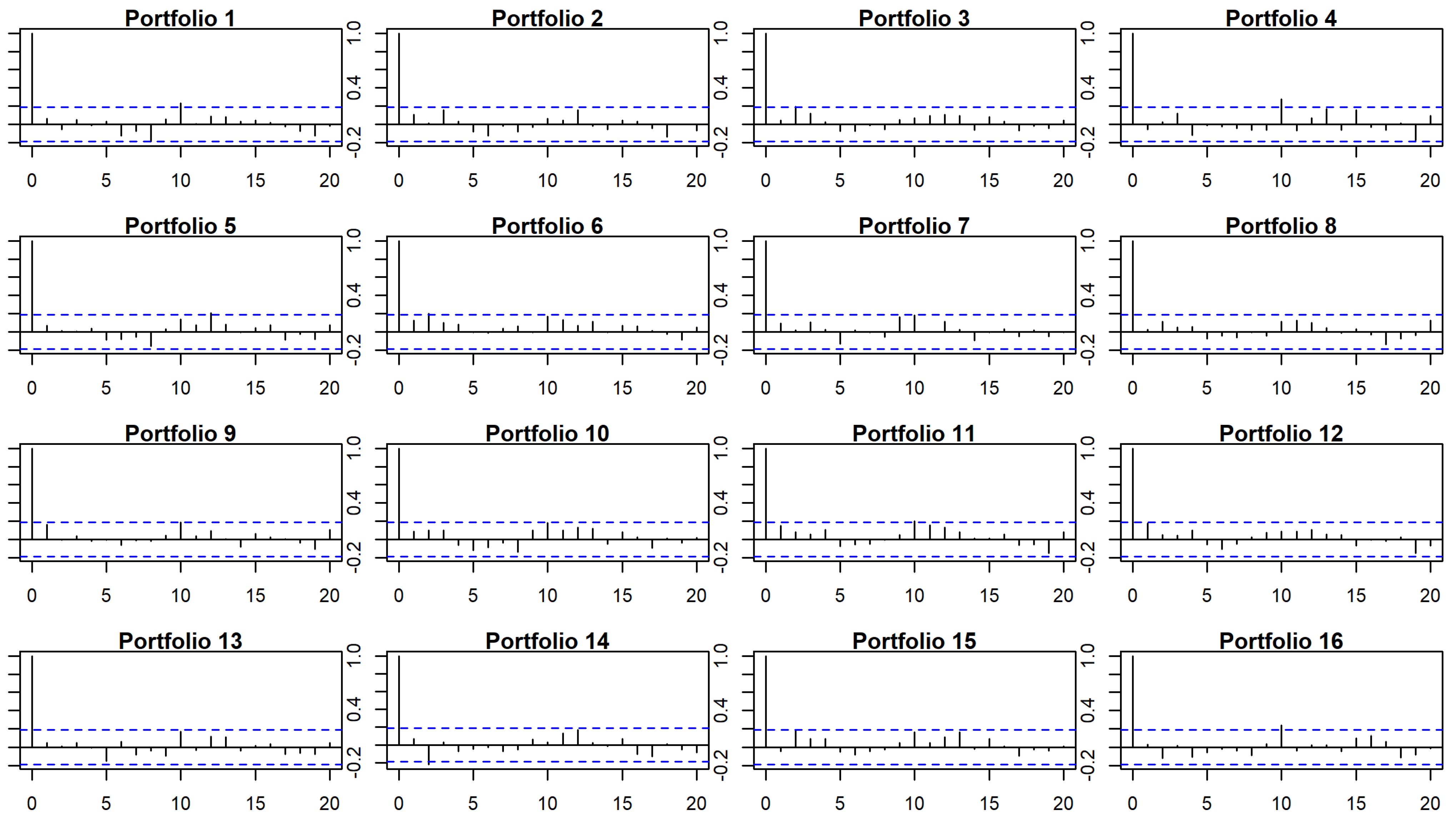
In Figure 5, we show the autocorrelation charts for errors in time-series regression for the 5-factor model for the whole period. According to the charts, residuals are correlated for lag equal to 10 and beyond. The Durbin-Watson test also suggests that errors may be autocorrelated for 12 portfolios for lag equal 10 when considering the whole period, 7 for the first subperiod and 7 for the second subperiod (p-values lower than $5\%$). In this case, incorporating the CPC-factors results in an increase in the number of portfolios that present autocorrelation.

Again, given that the three previous assumptions of the model are breached, resampling might be useful to approximate the distribution of the GRS statistic. When using the bootstrap, we cannot reject the hypothesis that all the $\alpha$s are jointly zero, since we find that $17.1\%$ of the values of the sample are higher than the GRS statistic. As in the previous case, the results obtained with the new statistic $Q\left(\alpha \right)$ reinforces our decision of not rejecting the hypothesis that all the $\alpha$s are jointly zero at a $5\%$ significance level.

In

Table 9. Results for Time-Series estimation of Model 2.

	Estimates						t-Statistics
Portfolio	$\mathbf{\alpha }$	Market	CPC1	CPC2	CPC3	CPC4	$\mathbf{\alpha }$	Market	CPC1	CPC2	CPC3	CPC4	Adj-${\mathit{R}}^{\mathbf{2}}$
1	0.001	0.436	−0.292	−0.381	0.626	0.687	0.731	6.674	−2.891	−1.503	3.029	6.199	0.688
2	0.002	0.286	−0.315	−1.601	0.497	1.607	0.693	3.819	−2.713	−5.497	2.092	12.621	0.825
3	0.000	0.290	−0.503	−1.257	0.719	0.288	−0.078	2.189	−2.453	−2.444	1.712	1.280	0.263
4	0.001	0.316	−0.547	−1.001	1.195	1.734	0.384	4.574	−5.127	−3.738	5.471	14.813	0.853
5	0.003	0.208	−0.311	−0.546	0.073	0.643	1.314	2.883	−2.791	−1.954	0.318	5.260	0.533
6	0.003	0.386	−0.592	0.358	−0.170	1.440	0.972	4.113	−4.072	0.981	−0.570	9.030	0.712
7	0.000	0.325	−0.303	−0.218	0.976	0.682	0.174	4.473	−2.690	−0.771	4.234	5.525	0.562
8	−0.001	0.306	−0.271	−0.598	1.428	1.654	−0.212	3.303	−1.896	−1.664	4.872	10.531	0.710
9	0.002	0.345	0.406	−0.879	0.625	0.832	1.129	5.021	3.821	−3.296	2.873	7.138	0.654
10	0.003	0.312	0.561	−1.874	0.442	1.368	1.225	3.784	4.404	−5.861	1.695	9.784	0.747
11	0.002	0.378	0.376	−1.018	1.040	0.659	1.084	5.254	3.376	−3.649	4.568	5.396	0.620
12	0.000	0.362	0.709	−0.871	0.948	1.670	0.195	4.622	5.854	−2.867	3.825	12.567	0.774
13	0.002	0.404	0.475	−0.025	0.478	0.640	0.885	5.457	4.150	−0.085	2.039	5.094	0.517
14	−0.001	0.259	0.370	−0.668	0.576	1.280	−0.220	2.679	2.469	−1.779	1.880	7.792	0.558
15	0.003	0.279	0.470	−0.302	0.414	0.679	1.416	3.489	3.802	−0.973	1.636	5.002	0.430
16	0.003	0.401	0.471	0.264	1.637	1.585	1.283	5.005	3.800	0.847	6.447	11.649	0.719

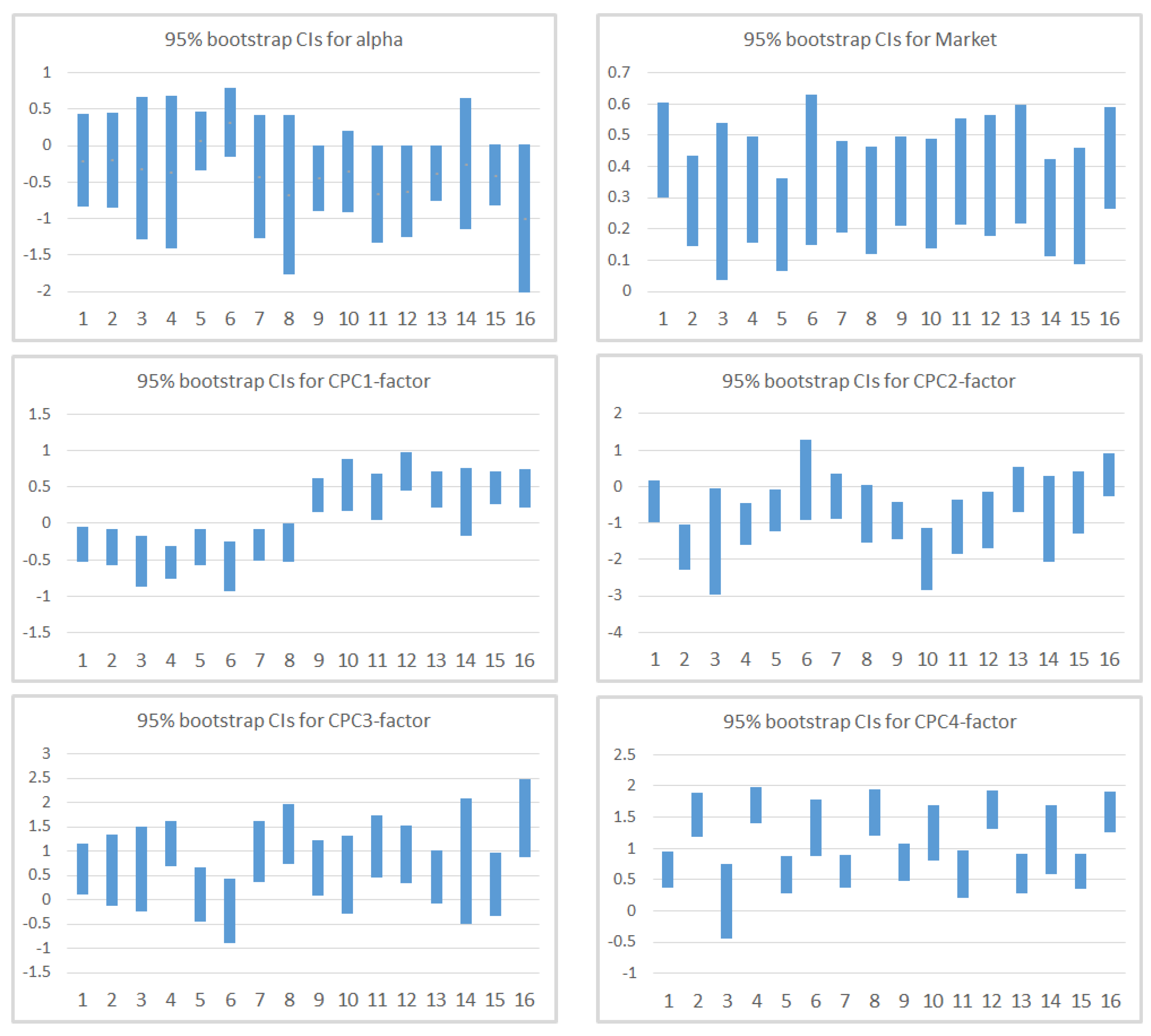
Notes. GRS: 2.242, p-value: 0.009, p-value Boot.: 0.171, p-value Q($\alpha$): 0.226.

, we present the results for the estimates and t-statistics for the classical methodology for Model 2. When we observe the coefficients ($\alpha$ and $\beta$) generated for the 16 portfolios, we notice that: (1) we cannot reject that each of the $\alpha$ are zero; (2) none of the Market $\beta$ can be considered statistically zero and the coefficients have stabilized around $0.35$ (as commented before, once we control for additional factors, and specifically for a factor linked to volatility, the Market $\beta$ effect that appeared in the previous model disappears); (3) $\beta$s for CPC1-factor and CPC4-factor seem to be significantly different from 0 as only 1 coefficient in each of them presents a t-statistic whose absolute value does not exceed $1.96$; and (4) the average adjusted-$R^2$ increases to $63.5\%$ (this model explains between $26.3\%$ and $85.3\%$ of the variation in the returns of the portfolios). CPC1-factor estimates are negative for portfolios with low mean and Momentum (CPC1), while the contrary happens in portfolios with high mean and Momentum (CPC1). Estimates for CPC2-factor are negative except for portfolios 6 and 16, and, in general, they are only significant for portfolios with low skewness and kurtosis (CPC2). Estimates for CPC3-factor are all positive except for portfolio 6. Finally, estimates for CPC4-factor are always positive and significant for all portfolios except for portfolio 3. Additionally, $\beta$s for CPC4-factor are higher for portfolios with high standard deviation (CPC4).

Table 10. Results for Bootstrap estimation of Model 2.

	Bootstrap CI (2.5%,97.5%)
Portfolio	$\mathbf{\alpha }$	Market	CPC1	CPC2	CPC3	CPC4
1	−0.840, 0.435	0.299, 0.605	−0.528, −0.044	−0.966, 0.179	0.105, 1.153	0.376, 0.945
2	−0.851, 0.452	0.145, 0.435	−0.582, −0.085	−2.288, −1.054	−0.129, 1.333	1.188, 1.888
3	−1.288, 0.666	0.038, 0.538	−0.869, −0.165	−2.966, −0.060	−0.236, 1.505	−0.453, 0.758
4	−1.410, 0.684	0.157, 0.496	−0.762, −0.315	−1.611, −0.462	0.680, 1.619	1.403, 1.978
5	−0.343, 0.473	0.065, 0.363	−0.567, −0.071	−1.242, −0.086	−0.461, 0.659	0.279, 0.876
6	−0.161, 0.797	0.147, 0.628	−0.930, −0.242	−0.916, 1.272	−0.900, 0.427	0.881, 1.785
7	−1.271, 0.413	0.190, 0.483	−0.518, −0.074	−0.894, 0.365	0.365, 1.622	0.363, 0.894
8	−1.770, 0.425	0.119, 0.465	−0.526, −0.006	−1.532, 0.035	0.732, 1.973	1.197, 1.938
9	−0.892, 0.008	0.209, 0.494	0.149, 0.623	−1.446, −0.413	0.091, 1.232	0.483, 1.067
10	−0.912, 0.201	0.137, 0.490	0.170, 0.879	−2.840, −1.137	−0.292, 1.313	0.809, 1.694
11	−1.329, 0.008	0.213, 0.554	0.052, 0.680	−1.854, −0.372	0.445, 1.737	0.212, 0.968
12	−1.255, 0.005	0.177, 0.566	0.453, 0.980	−1.680, −0.145	0.332, 1.513	1.316, 1.931
13	−0.759, 0.008	0.216, 0.596	0.221, 0.720	−0.708, 0.548	−0.082, 1.022	0.274, 0.907
14	−1.154, 0.646	0.114, 0.424	−0.166, 0.753	−2.052, 0.300	−0.491, 2.086	0.581, 1.698
15	−0.821, 0.010	0.087, 0.458	0.260, 0.706	−1.298, 0.412	−0.343, 0.966	0.351, 0.910
16	−2.012, 0.010	0.265, 0.589	0.210, 0.751	−0.252, 0.906	0.876, 2.468	1.254, 1.916

contains the results for the inference based on resampling techniques. A graphical comparison is shown in Figure 6. The results of the basic bootstrap confidence intervals are consistent with what we have already commented. Despite having a lower GRS p-value than Model 1, we can conclude that this model is better as (1) resampling techniques show that we cannot reject that $\alpha$s are jointly zero; (2) the average adjusted-$R^2$ increases; (3) Market $\beta$s change and stabilize around $0.35$; and (4) factors based on mean and Momentum (CPC1-factor) and standard deviation (CPC4-factor) only present 1 non-significant portfolio.

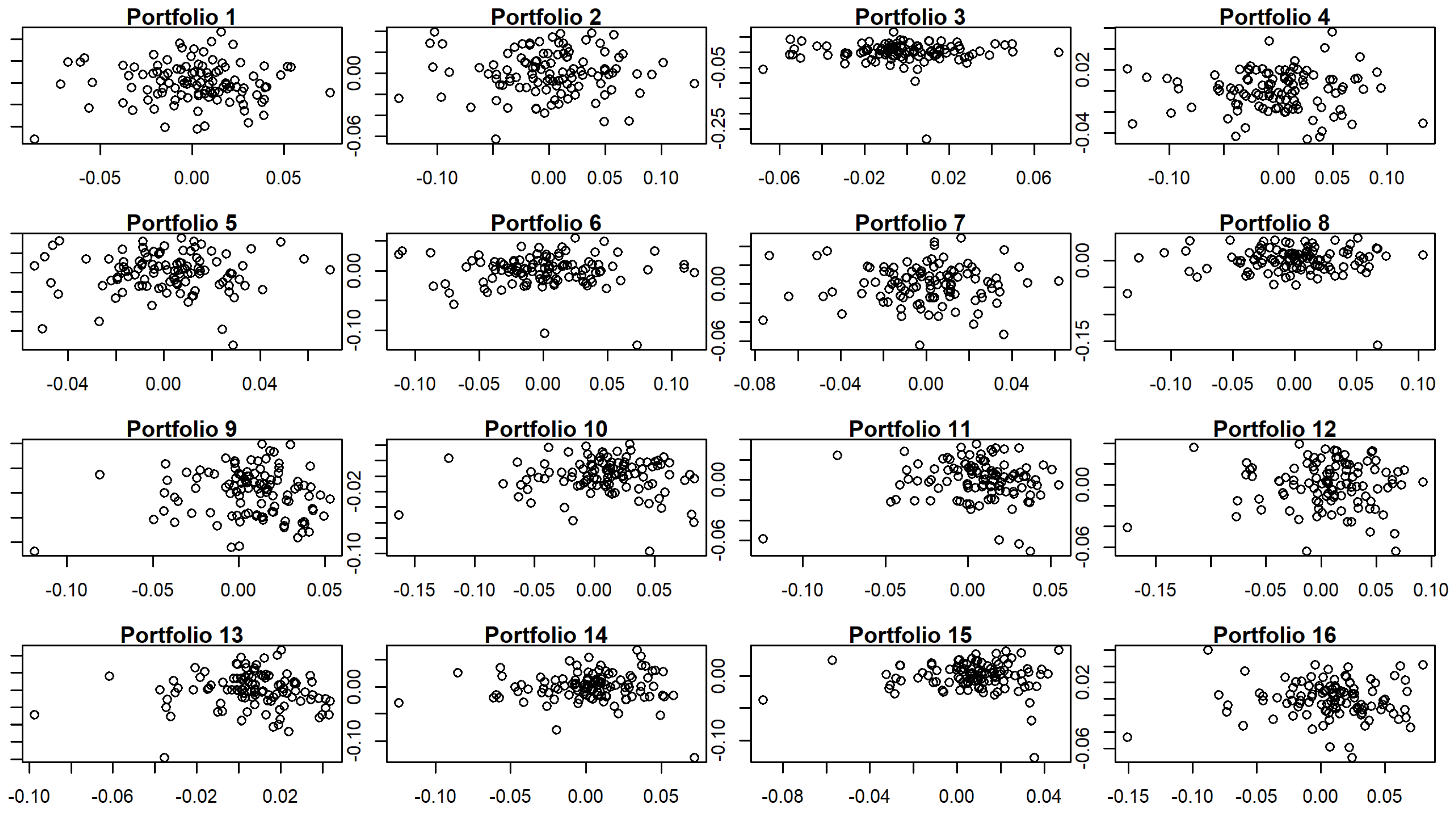
We noticed that some of the intervals seem to be quite wide. Specifically, intervals for portfolio 3 are all wider than their respective averages and the z-score of the width of 3 of them is higher than 2. Those of portfolio 14 are equally wider than their means, with the exception of the interval for Market $\beta$ (in this case, the z-score of the width is higher than 2 in only 2 of the intervals ). Additionally, in both cases, adjusted $R^2$ is lower than the average. The explanation for both portfolios may be, among others, the existence of outliers that impact the width of the bootstrap intervals in the simulations; see Figure 7.

Next, we will proceed to analyze the significance of the different risk premia for both models.

3.2. Cross-Sectional Regression

In this section, we present the results for the cross-section regression of the two models under study: CAPM (Model 1) and the five-factor model, including Market and factors CPC1 to CPC4 (Model 2).

3.2.1. Model 1: CAPM

The GRS bootstrap test for Model 1 suggests that we cannot reject that all $\alpha$s are jointly zero and further it registers an explained variability between $19\%$ and $52.6\%$. Market seems to be statistically significant in all the portfolios.

We use the $\beta$s estimated in Table 7 to examine if the factor is priced on the cross-section of returns. We must take into account that despite the fact that we are working with portfolios, risk premia will be estimated from the estimated coefficients, which can lead to an important bias, especially if the model is not well specified.

Market’s risk premium is $0.0043$ per month and, as a consequence, returns depend positively on the Market. The reported t-statistic of $0.874$, which in this case includes the Shanken correction [31], suggests that this factor is not statistically significant at a $5\%$ significance level. The correction seems to be minor in this case, as the t-statistic for the simple regression (Fama-Macbeth approach) is $0.8776$. The basic bootstrap confidence interval [−0.0078, 0.0015] confirms that this factor is not statistically significant during the considered period. The statistical non-significance of the Market factor despite its wide confirmation in the financial literature could be related to the fact that we are not controlling for other factors, as the results from Model 2 suggest.

3.2.2. Model 2: Market and Factors CPC1 to CPC4

Again, we use the estimated $\beta$s for Model 2 (see Table 9) to examine if the different factors are priced on the cross-section of returns and the results are reported in

Table 11. Results for Cross-Sectional estimation of Model 2.

		t-Statistic		Bootstrap
	Estimate	FM	CS	$\mathbf{95}\%$CI
Market	0.0108	2.054	1.5447	0.0091, 0.0254
CPC1	0.0071	9.625	3.5836	0.0017, 0.0181
CPC2	−0.0001	−0.085	−0.0502	−0.0126, 0.0038
CPC3	−0.0012	−2.241	−1.1303	−0.0150, 0.0014
CPC4	0.0002	0.445	0.1139	−0.0120, 0.0043

.

The highest risk premia are those of Market, which is $0.0108$, and the one associated with the factor based on mean and Momentum (CPC1-factor), which is $0.0071$. In both cases, returns depend positively on them. The rest of the risk premia are much lower and non-significant at $5\%$ significance levels both for traditional methods and resampling techniques. The reported t-statistics, which in the case of CS include the Shanken correction, suggest that the only statistically significant factor at conventional significance levels is that based on mean and Momentum (CPC1-factor). However, bootstrap intervals indicate that both Market and CPC1-factor $\lambda$s are significantly different from zero (at 5% level) contributing to the model. This is consistent with the 4-factor model by Carhart [11]. Additionally, once we control for a volatility factor (CPC4), we notice that expected returns, at least during the period considered, do not depend on standard deviation. See Reference [33] for potential explanations and a historical review of the volatility effect.

3.3. Comparison between Classical Methodologies and Bootstrap Methods

As we have seen, the assumptions’ violation of the residuals of the regressions, like non-normality, heteroskedasticity, and autocorrelation, as well as, the presence of multicollinearity (that is, high correlation among the different factors used in the analysis), may affect the estimates of $\alpha$, ${\beta }_i$ and GRS computed through classical methodologies.

Table 12. Comparison of classical methodologies and bootstrap methods.

		Number of Portfolios Where
Model	Factors	${\mathbf{\beta }}_{\mathit{m}}=\mathbf{0}$	${\mathbf{\beta }}_{\mathit{CPC}\mathbf{1}}=\mathbf{0}$	${\mathbf{\beta }}_{\mathit{CPC}\mathbf{2}}=\mathbf{0}$	${\mathbf{\beta }}_{\mathit{CPC}\mathbf{3}}=\mathbf{0}$	${\mathbf{\beta }}_{\mathit{CPC}\mathbf{4}}=\mathbf{0}$	GRS p-Value	Adj-${\mathit{R}}^{\mathbf{2}}$
Model 1	Market	0	-	-	-	-	0.019	0.190 to 0.526
Model 1b	Market	0	-	-	-	-	0.174
Model 2	Market & CPCs	0	1	9	6	1	0.009	0.263 to 0.853
Model 2b	Market & CPCs	0	1	8	8	1	0.171

contains a comparison between the inferential results obtained with both methodologies. In particular, we show the number of portfolios where ${\beta }_i=0$. Rows corresponding to Model 1 and Model 2 contain classical inferential results, whereas rows Model 1b and Model 2b contain bootstrap inferential results. Indeed, looking at those results, we notice that the p-values of the bootstrap GRS tests are always greater than those of classical procedures, showing that the former are more conservative (we fail to reject the null hypothesis that the $\alpha$ are jointly 0 more often). We also observe that the number of portfolios where ${\beta }_i=0$ varies depending on the methodology used.

4. Conclusions

We propose a procedure to obtain and test multifactor models based on statistical and financial factors and illustrate it on a large dataset corresponding to nearly 1250 EU companies and spanning from October 2009 to October 2019. However, the procedure is general enough to be extended to other factors, companies or time period.

The first methodological contribution relies on using Common Principal Components to build the portfolios and summarize factors’ information by capturing a high percentage of the variability of the datasets. In this paper, we considered factors like Market Capitalization and Total Assets (measures of size), Price to Book ratio (measure of cheapness), Return on Assets and Return on Equity (measures of profitability), Momentum, and four statistical measures, such as mean, standard deviation, kurtosis, and skewness. The second methodological contribution is the development of a block-bootstrap procedure to assess the validity of the model and the significance of the parameters involved.

The main findings indicate that the multifactor model proposed improves the Capital Asset Pricing Model with regard to the adjusted-$R^2$ in the time-series regressions. Cross-section regression results reveal that Market and a factor related to Momentum and mean of stocks’ returns have positive risk premia for the analyzed period. Finally, we also observe that tests based on block-bootstrap statistics are less prone to reject the validity of the model than classical procedures.

In this paper, we proposed Common Principal Components to obtain multifactor models for equity returns, mainly because it can deal with several datasets and can be applied to non-normal data. Direct extensions of this work are to explore the efficency of these multifactor models in other equity markets, as well as in other time periods. A further research line is to explore and adapt other multivariate dimensionality reduction techniques, like MANOVA, although this technique requires additional hypothesis that are hardly fulfilled in real datasets. To explore and adapt MANOVA to be used in large datasets is beyond the scope of this paper, and we leave it for further research.

References

- Sharpe, W.F. Capital asset prices: A theory of market equilibrium under conditions of risk. J. Financ. 1964, 19, 425–442. [Google Scholar]
- Lintner, J. The valuation of risk assets and the selection of risky investments in stock portfolios and capital budgets. Rev. Econ. Stat. 1965, 47, 13–37. [Google Scholar] [CrossRef]
- Mossin, J. Equilibrium in a Capital Asset Market. Econometrica 1966, 34, 758–783. [Google Scholar] [CrossRef]
- Frazzini, A.; Pedersen, L. Betting agains beta. J. Financ. Econ. 2014, 111, 1–25. [Google Scholar] [CrossRef] [Green Version]
- Miller, M.H.; Scholes, M. Rates of return in relation to risk: A reexamination of some recent findings. In Studies in the Theory of Capital Markets; Jensen, M.C., Ed.; Praeger: New York, NY, USA, 1972; pp. 47–78. [Google Scholar]
- Fama, E.F.; French, K.R. The cross-section of expected returns. J. Financ. 1992, 47, 427–465. [Google Scholar] [CrossRef]
- Viale, A.M.; Kolari, J.W.; Fraser, D.R. Common risk factors in bank stocks. J. Bank. Financ. 2009, 33, 464–472. [Google Scholar]
- Ramos, S.; Taamouti, A.; Veiga, H.; Wang, C.W. Do investors price industry risk? Evidence from the cross-section of the oil industry. J. Energy Mark. 2017, 10, 79–108. [Google Scholar] [CrossRef] [Green Version]
- Elyasiani, E.; Gambarelli, L.; Muzzioli, S. Moment risk premia and the cross-section of stock returns in the European stock market. J. Bank. Financ. 2020, 111, 105732. [Google Scholar] [CrossRef]
- Lemperiere, Y.; Deremble, C.; Nguyen, T.; Seager, P.; Potters, M.; Bouchaud, J. Risk Premia: Asymmetric Tail Risks and Excess Returns. Quant. Financ. 2017, 17, 1–14. [Google Scholar]
- Carhart, M.M. On Persistence in Mutual Fund Performance. J. Financ. 1997, 52, 57–82. [Google Scholar] [CrossRef]
- Misra, A.; Mohapatra, S. Evidence and Sources of Momentum Profits. A Study on Indian Stock Market. Econ. Manag. Financ. Mark. 2014, 9, 86–109. [Google Scholar]
- Harvey, C.; Liu, Y.; Zhu, H. ... and the cross-section of expected returns. Rev. Financ. Stud. 2015, 29, 5–68. [Google Scholar] [CrossRef] [Green Version]
- Fama, E.F.; French, K.R. Choosing factors. J. Financ. Econ. 2018, 128, 234–252. [Google Scholar] [CrossRef]
- Barillas, F.; Shanken, J. Which alpha? Rev. Financ. Stud. 2017, 30, 1316–1338. [Google Scholar] [CrossRef]
- Fama, E.F.; French, K.R. A five-factor asset pricing model. J. Financ. Econ. 2015, 116, 1–22. [Google Scholar] [CrossRef] [Green Version]
- Heerden, J.V.; Rensburg, P.V. Common Firm-Specific Characteristics of Extreme Performers on The Johannesburg Securities Exchange. Econ. Manag. Financ. Mark. 2017, 12, 25–50. [Google Scholar]
- Feng, G.; Giglio, S.; Xiu, D. Taming the Factor Zoo: A Test of New Factors. J. Financ. 2020, 75, 1327–1370. [Google Scholar] [CrossRef]
- Flury, B.N. Common principal components in k groups. J. Am. Stat. Assoc. 1984, 79, 892–898. [Google Scholar] [CrossRef]
- Fama, E.F.; French, K.R. Common risk factors in the returns on stocks and bonds. J. Financ. Econ. 1993, 33, 3–56. [Google Scholar] [CrossRef]
- Fama, E.F.; MacBeth, J.D. Risk, Return and Equilibrium: Empirical Tests. J. Political Econ. 1973, 81, 607–636. [Google Scholar] [CrossRef]
- Efron, B. Bootstrap Methods: Another Look at the Jackknife. Ann. Stat. 1972, 7, 1–26. [Google Scholar]
- Cueto, J.M.; Grané, A.; Cascos, I. Models for Expected Returns with Statistical Factors. J. Risk Financ. Manag. 2020, 13, 314. [Google Scholar] [CrossRef]
- Chou, P.; Zhou, G. Using Bootstrap to Test Portfolio Efficiency. Ann. Econ. Financ. 2006, 1, 217–249. [Google Scholar]
- Grané, A.; Veiga, H. Accurate minimum capital risk requirements: A comparison of several approaches. J. Bank. Financ. 2008, 32, 2482–2492. [Google Scholar] [CrossRef]
- Flury, B.N.; Gaustchi, W. An algorithm for simultaneous orthogonal transformation of several positive definite symmetric matrices to nearly diagonal form. SIAM J. Sci. Stat. Comput. 1986, 7, 169–184. [Google Scholar] [CrossRef]
- Flury, B. Common Principal Components and Related Multivariate Models; John Wiley & Sons: Hoboken, NJ, USA, 1988. [Google Scholar]
- Breiman, L. Bagging predictors. Mach. Learn. 1996, 24, 123–140. [Google Scholar] [CrossRef] [Green Version]
- Gibbons, M.R.; Ross, S.A.; Shanken, J. A test of the efficiency of a given portfolio. Econometrica 1989, 57, 1121–1152. [Google Scholar] [CrossRef] [Green Version]
- Fama, E.F. Cross-Section Versus Time-Series Tests of Asset Pricing Models. Fama-Mill. Work. Pap. 2015. [Google Scholar] [CrossRef]
- Shanken, J. On the estimation of beta-pricing models. Rev. Financ. Stud. 1992, 5, 1–33. [Google Scholar] [CrossRef]
- Soumaré, I.; Aménounvé, E.J.; Diop, O.; Méité, D.; N’Sougan, Y.D. Applying the CAPM and the Fama-French models to the BRVM stock maket. Appl. Financ. Econ. 2013, 23, 275–285. [Google Scholar] [CrossRef]
- Blitz, D.; Falkenstein, E.; van Vliet, P. Explanations for the Volatility Effect: An Overview Based on the CAPM Assumptions. J. Portf. Manag. 2014, 40, 61–76. [Google Scholar] [CrossRef]
Figure 1.
Summary statistics of the data by year.
Figure 2.
Portfolios’ cumulative returns.
Figure 3.
Autocorrelation charts for errors in TS regression for CAPM for the whole period.
Figure 4.
Graphical comparison of 95% Bootstrap CIs for Model 1.
Figure 5.
Autocorrelation charts for errors in TS regression for 5-factor model for the whole period.
Figure 6.
Graphical comparison of 95% Bootstrap CIs for Model 2.
Figure 7.
Residuals vs. fitted values in TS regression for 5-factor model for the whole period.