Analysis of Instantaneous Feedback Queue with Heterogeneous Servers


1
Institute of Control Systems, Department of Teletraffic Theory, National Academy of Science, Baku AZ 1148, Azerbaijan
2
Faculty of Applied Mathematics and Cybernetics, Baku State University, Baku AZ 1148, Azerbaijan
3
Department of Informatics and Networks, Faculty of Informatics, University of Debrecen, 4032 Debrecen, Hungary
*
Author to whom correspondence should be addressed.
Mathematics 2020, 8(12), 2186; https://doi.org/10.3390/math8122186
Submission received: 12 November 2020
/
Revised: 5 December 2020
/
Accepted: 7 December 2020
/
Published: 8 December 2020
(This article belongs to the Special Issue Stochastic Modeling and Applied Probability)
Abstract
:A system with heterogeneous servers, Markov Modulated Poisson flow and instantaneous feedback is studied. The primary call is serviced on a high-speed server, and after it is serviced, each call, according to the Bernoulli scheme, either leaves the system or requires re-servicing. After the completion of servicing of a call in a slow server, according to the Bernoulli scheme, it also either leaves the system or requires re-servicing. If upon arrival of a primary call the queue length of such calls exceeds a certain threshold value and the slow server is free, then the incoming primary call, according to the Bernoulli scheme, is either sent to the slow server or joins its own queue. A mathematical model of the studied system is constructed in the form of a three-dimensional Markov chain. Approximate algorithms for calculating the steady-state probabilities of the models with finite and infinite queues are proposed and their high accuracy is shown. The results of numerical experiments are presented.
1. Introduction
When building mathematical models of communication processes, as well as processes related to the processing of parts in production systems, inventory management processes, etc., it becomes necessary to take into account the repeated processing of some calls. For example, in many information transmission systems, erroneously transmitted data (packets, frames, etc.) are re-transmitted, since the performance of such systems is often evaluated by the reliability of data transmission. Similarly, in manufacturing systems, if the parts produced have certain defects, then in some situations they need to be re-processed.
Taking into account that the effect of repeated call servicing leads to the need to use models of systems with feedback (Feed Back Queue, FBQ), such models were first introduced in [1,2]. It is necessary to distinguish between Instantaneous Feed Back Queue (IFBQ) systems, where a retry occurs immediately after the service is complete, and Delayed Feed Back Queue (DFBQ) systems, in which a replay of a service request occurs after a certain positive time.
The current state of the problem of studying FBQ models is described in detail in [3], so here, we will not dwell on the presentation of the results known in this direction. In this work, it is noted that the overwhelming majority of works study FBQ models without a buffer for waiting for calls. At the same time, in many systems, buffers are organized for waiting of calls in queue. Therefore, to adequately describe the operation of such systems, it becomes necessary to study FBQ models with buffers.
Based on the above facts, in this paper we study the IFBQ model with buffers. Note that there are few works in the available literature devoted to the study of such models. Among them, we note the works [4,5,6,7,8,9,10,11,12,13]. Simple one-dimensional IFBQ models with one server and impatient calls using various mechanisms for keeping them in the queue at the moments of the end of the admissible waiting time are studied in [4,5,6,7,8,9,10]. A model with two heterogeneous servers and a bounded queue, in which incoming calls with known probabilities are assigned to the servers, was studied in [11]. Note that in [4,5,6,7,8,9,10,11] the primary calls and the calls that require repeated servicing are not distinguished. Therefore, using the approach proposed in them, it is impossible to find the distribution of the number of calls that require repeated servicing. A more complex IFBQ model with one server and bounded queue was studied in [12], where the incoming stream is a Markov Arrival Process (MAP) stream and the service time of calls has a phase-type distribution function. It is shown that the mathematical model of the system is a certain four-dimensional Markov Chain (MC) and the performance measures of the system are calculated. In the recent work [13], the IFBQ model with one server and two Poisson streams was studied. It is considered that for each type of call there are separate buffers of infinite size, while only high priority calls can repeat requests for servicing, according to the Bernoulli scheme. It is assumed that calls that require re-servicing are sent to the queue of low priority calls, while models with preemptive and non-preemptive priorities are studied. In [12,13], the matrix-geometric method [14] is used to study the proposed models.
An analysis of the available works showed that they are based on a number of assumptions. The main ones are the following: (1) initial and repeated applications are identical in all respects; (2) calls can only repeat a request once for service; (3) calls of both types (primary and secondary or feedback calls) are transmitted by a single server.
However, in many real systems, these assumptions are not met, and therefore, in order to improve the adequacy of the models, this work studies an IFBQ in which the above assumptions are not met. In this case, it is assumed that the servers are specialized in the type of requests, and they are heterogeneous, i.e., have different service rates (earlier systems with heterogeneous servers in the absence of feedback were studied in many works, see, for example, [15] and its bibliography). In addition, in contrast to the standard assumption that the incoming stream is Poisson, here we study a model with a Markov Modulated Poisson Process (MMPP) stream [16]. Note that the proposed model is studied using the method of hierarchical space merging of a multi-dimensional MC [17]. Application of this method makes it possible to develop effective numerical procedures for calculating the performance measures of the system under study.
The paper is structured as follows. Section 2 contains a description of the system under study and a statement of the problem. In Section 3, a mathematical model of the system in the form of a 3D MC is developed and its generating matrix is determined. Here, the ergodicity condition of the model is obtained and an approximate method for calculating the steady-state probabilities and performance measures of the system is developed. Section 4 presents the results of numerical experiments. Concluding remarks are given in Section 5.
2. Description of the System with Instantaneous Feedback and Formulation of the Problem
As in [17], it is assumed that input flow is MMPP with parameters . This means that the MC, which controls the intensities of the incoming flow, has a generating matrix (GM) of dimension , where determines the transition intensity from state to state , , and . It is assumed that when MC is in a state , the intensity of the incoming stream is equal to , and when the state of the MC changes, the intensity of the incoming flow also changes instantly. The vector of intensities of the incoming flow is denoted by .
The system contains two servers, a high-speed (F-server) and a low-speed (S-server) server, while primary calls (p-calls), as a rule, are served in the F-server; after the completion of servicing, the p-calls, according to the Bernoulli scheme or with probability , leave the system, or, with probability , are sent to be served in the S-server. Calls that require re-servicing (secondary calls, s-calls) can queue up in front of the S-server. It is assumed that s-calls can repeatedly require re-servicing, i.e., after the completion of service, each s-call is independent of other calls according to the Bernoulli scheme or with the probability leaves the system permanently or with a complementary probability instantly requires re-servicing in the S-server. The service times of calls in the F-server and in the S-server are random variables that have an exponential distribution with parameters and , respectively, where .
If at the moment of receipt of a p-call the number of calls in the queue in front of the F-server is higher than a certain threshold value, , and at the same time the S-server is not busy, then the received p-call either with probability is sent for service to the S-server or with a complementary probability it joins its queue.
Serving different types of calls and changing the states of the MC, which controls the intensity of the incoming flow, are random processes independent of each other.
The problem is to find the joint distribution of the states of the MMPP flow and the number of calls of each type in the system. The solution to this problem will allow us to find the performance measures of the system, i.e., the average number of p-calls and s-calls in the system and the intensity of p-calls served in the S-server .
3. Calculation of the Steady-State Probabilities and Performance Measures
The state of the system is determined by the 3D vector , where is the state of the MC that controls the intensity of the incoming flow, is the total number of calls in front of the F-server and calls in it, and is the total number of calls in front of the S-server and calls in it. Then, the state space of this 3D MC is defined as the Cartesian product of three sets:
The intensity of transition from state to state will be denoted by . These values are calculated as follows:
- transitions are carried out with intensity when the state of the MC that controls the intensity of the incoming MMPP flow changes;
- transitions and are carried out with intensity when a p-call arrives;
- transitions are carried out with intensity when a p-call arrives;
- transitions are carried out with intensity when a p-call arrives;
- transitions are carried out with intensity upon completion of servicing the p-call in the F-server and leaving the system;
- transitions are carried out with intensity upon completion of servicing the p-call in the F-server and returning to the S-server for re-servicing;
- transitions are carried out with intensity upon completion of servicing the p-call in the S-server.
Therefore, the positive elements of the GM of the given 3D MC are determined from the following relations:
Let us denote by the probability of state . The condition for the existence of a stationary regime is obtained below.
Finding the steady-state probabilities is sufficient to calculate the performance measures of the system under study. Thus, the average number of p-calls and s-calls in the system are defined as the mathematical expectation of the corresponding random variables:
The intensity of p-calls, which are served in the S-server , is defined as:
Using the method of multidimensional generating functions to find the steady-state probabilities faces a number of methodological and computational difficulties. On this basis, below is described an alternative method for solving this problem, based on the hierarchical space merging method of a multidimensional MC [17].
By taking into account that changing the states of the MC, which controls the intensity of the incoming flow, are independent on other parameters of the system, consider the following splitting of the state space (1):
where
All states from the class are combined into one merged state, , and on the basis of splitting (6) in the state space (1), the merge function is determined. Let us denote the set of merged states by
Then, the approximate values of the steady-state probabilities of the original model, denoted by are defined as (see [17])
where is the probability of the state inside a split model with state space , and is the probability of the merged state
As noted above, the transitions between the states of the MC that control the intensity of the incoming flow do not depend on the statuses of the F-server and S-server, and therefore, the probabilities of the states are defined by its GM . Consequently, to find the steady-state probabilities of the original model, we only need to determine the stationary distributions of a 2D MC with state spaces (see Formula (7)). To solve this problem, a merge procedure (second level of the hierarchy) is applied to this 2D MC. Since all split models with state spaces have identical GM, then we fix the value of the parameter .
Below we assume that and , i.e., and , and consider the following partition in the class :
where .
In accordance with the above accepted assumptions, transition intensities between states within each split class are essentially larger than transition intensities between states from different splitting classes. On the basis of splitting (8), all states from class are combined into one merged state , and in the state space the merge function is determined. Let us denote the set of merged states by
According to [17], we have:
where is the probability of the inside a split model with state space , and is the probability of the merged state
In class in the all state vectors, the second component is to . Therefore, when studying the split models with space , every state can only be specified by the first component, i.e., in further the states are denoted as . Then, from relations (2) we conclude that the intensities of transitions between the states of the split model with the state space depend on the parameter and are defined as follows:
Case
Cases
From (10) we obtain that under the fulfilling of the condition state probabilities of a split model with state space are defined as follows:
where is determined from the normalization condition, i.e., After standard transformations we get
Remark 1.
Since the conditionis satisfied for every, then we get that the following condition must be satisfied:
From (11) we obtain that under the fulfilling of the condition, state probabilities of split models with state spacesare not dependent on indexand are determined as follows:
Remark 2.
Since the conditionshould be satisfied for each, then we get that the following condition must be satisfied:
Then, combining conditions (14) and (16), we obtain the first ergodicity condition for the model, i.e., condition (16) must be satisfied.
Taking into account (2), (12), (13), and (15), we obtain that the intensities of transitions between statesare defined as
Taking into account (12) and (13), the valuein Formula (17) is defined as follows:
From (17) we obtain that under the conditionstate probabilities of a merged model with a state spaceare defined as follows:
whereandis determined from the normalization condition, i.e.,After standard transformations we get
Remark 3.
Since the conditionshould be satisfied for each, then we obtain the second ergodicity condition of the model:
Combining relations (16) and (20), we obtain the following condition for the ergodicity of the model:
Remark 4.
From (21) we conclude that the ergodic condition does not depend on the parameters of the GM of the MC that controls the intensity of the MMPP flow.
Thus, when the ergodicity condition of model (21) is satisfied, taking into account relations (7), (9), (12), (13), (18), and (19), the approximate values of the steady-state probabilities of the original 3D MC are found.
Further, using steady-state probabilities, approximate values of performance measures (3)–(5) can be calculated. Indeed, from (7) and (9) we conclude that these performance measures are calculated as follows:
Then, after certain mathematical calculations from (22)–(24) we get
where
It is important to note that the proposed approach can be used to analyze a similar model with limited buffers in front of servers of different types. Indeed, let the sizes of buffers in front of flow and slow servers be equal to and , respectively.
The state space of this model is finite-dimensional and is defined as Elements of the GM of the corresponding 3D MC are defined similarly to relation (2) by taking into account that .
Note that for any positive values of the initial parameters of the system, a stationary mode exists in this Markov chain, since it is irreducible and has a finite state space. In this model, along with performance measures (3)–(5), a new measure appears, i.e., the probability of losing p-calls, . It is defined as follows:
To find the steady-state probabilities of the appropriate 3D MC, an exact method based on the use of a system of equilibrium equations can be used here. This approach is effective only for models of moderate dimensions. For large-scale models, the approximate approach described above can be used.
Let’s briefly consider the applications of the approximate approach. Here, splitting (6) is also considered at the first level of the hierarchy, and splitting (8) is used at the second level of the hierarchy, but it is taken into account that the infinity sign is replaced by the parameter Probabilities of states inside split classes are calculated as follows:
Case
where ;
Cases
The probabilities of merged states in this model are determined similarly to (18). The normalizing constant, , in this model is determined from the normalization condition, i.e., Further, as above, using Formula (29)–(31), the steady-state probabilities are determined and the approximate values of the performance measures of the system (3)–(5) and (28) are calculated.
4. Numerical Results
For the sake of brevity, we consider here the results of numerical experiments only for the model with infinite buffers. Numerical experiments carried out here have two purposes: (1) to show the high accuracy of the developed algorithm for the approximate calculation of steady-state probabilities of the system under study; (2) to study the behavior of the performance measures of the system with respect to changes in the threshold parameter .
The accuracy of the approximate algorithm is estimated using simulation. In this case, the closeness of the results obtained using different approaches is estimated using the cosine similarity norm, i.e.,
where and are vectors of exact and approximate values of steady-state probabilities, respectively, denotes the dot product of vectors and ; and are the magnitudes of vectors and respectively.
Note that, as a rule, the cosine similarity norm is used to determine the orientation of two vectors, and not to compare their values. However, in our case, this measure adequately estimates the proximity of the end points of the vectors and , since according to the normalizing condition we have ; in other words, the endpoints of these vectors are in the same hyper plane.
First, consider the case when the values of the rates of the incoming flow are fixed, but the rates of service for different types of servers change. In this case, in the experiments carried out, the initial data of the hypothetical model are determined as follows. The GM of the MC with three states that controls the intensity of the incoming MMPP flow is defined as:
The values of incoming flow rates are . The parameters of Bernoulli schemes were chosen as follows:
Comparative analysis of the results of the approximate algorithm and the simulation method for this series of computational experiments are shown in Table 1. We also performed computational experiments for the cases when the values of the rates of the incoming flow and the rate of service of different types of servers change. In three series of experiments, the parameters of the Bernoulli scheme remained unchanged. In the first series of experiments, the GM of MC with three states that controls the intensity of the incoming MMPP flow was chosen in the same way as before (i.e., it is equal to ); in this case, the values of the intensities of the incoming flow were chosen as . In the second and third series of experiments, the GM of MC with three states that control the intensities of the incoming MMPP flow and the corresponding values of the intensities of the incoming flow were chosen as follows:
The results of these experiments are shown in Table 2. Table 1 and Table 2 show that the developed algorithm has high accuracy, since the value of the norm (31) is practically equal to one.
Remark 5.
Since the system is infinite-dimensional (with respect to the second and third components of the state vector), when calculating the norm (31), the maximum number of calls of each type in the system from above is limited by sufficiently large finite values. Such a replacement is justified, since when these values exceed certain (sufficiently large) values, the corresponding state probabilities become infinitely small values, i.e., practically equal to zero.
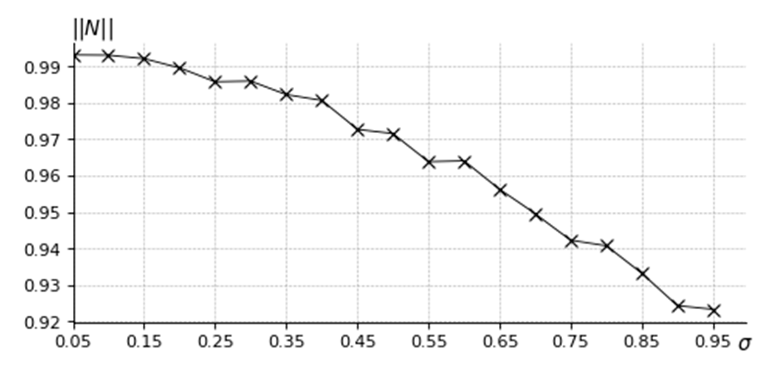
The developed approximate formulas also make it possible to study the behavior of the similarity norm (31) with respect to changes in any (structural and load) parameters of the system. Due to the limited scope of work and for the sake of concreteness, only the results are presented here that show the behavior of this quantity with respect to the change in the parameter . The corresponding results are shown in Figure 1. It can be seen from the graph that with an increase in the value of this parameter, the accuracy of the formulas for calculating the approximate values of the steady-state probabilities of the original 3D MC deteriorates. In other words, the smaller the value of the specified parameter, the higher the accuracy of the proposed formulas. However, even in the worst cases, when the values of this parameter are close to unity, the values of norm (31) turn out to be greater than 0.9, i.e., the developed approximate formulas have a sufficiently high accuracy.
This behavior of norm (31) with respect to a parameter has a completely logical explanation. Indeed, it is known from the theory of space merging of MCs [3] that the lower the intensity of transitions between split classes of states, the higher the accuracy of the space merge algorithms. For the model studied here, at small values of the parameter , the intensities of transitions between split classes (see Formula (8)) turn out to be small, and with its growth the intensity of transitions between split classes increases.
Note that a similar behavior of norm (31) is observed with respect to changes in the parameters and , i.e., with increasing of parameter the value of the norm is systematically increasing, while with increasing of parameter , on the contrary, it systematically decreases (note that, in contrast to parameter , ranges of change in parameters and and are determined from the ergodicity condition for the system, see (21)).
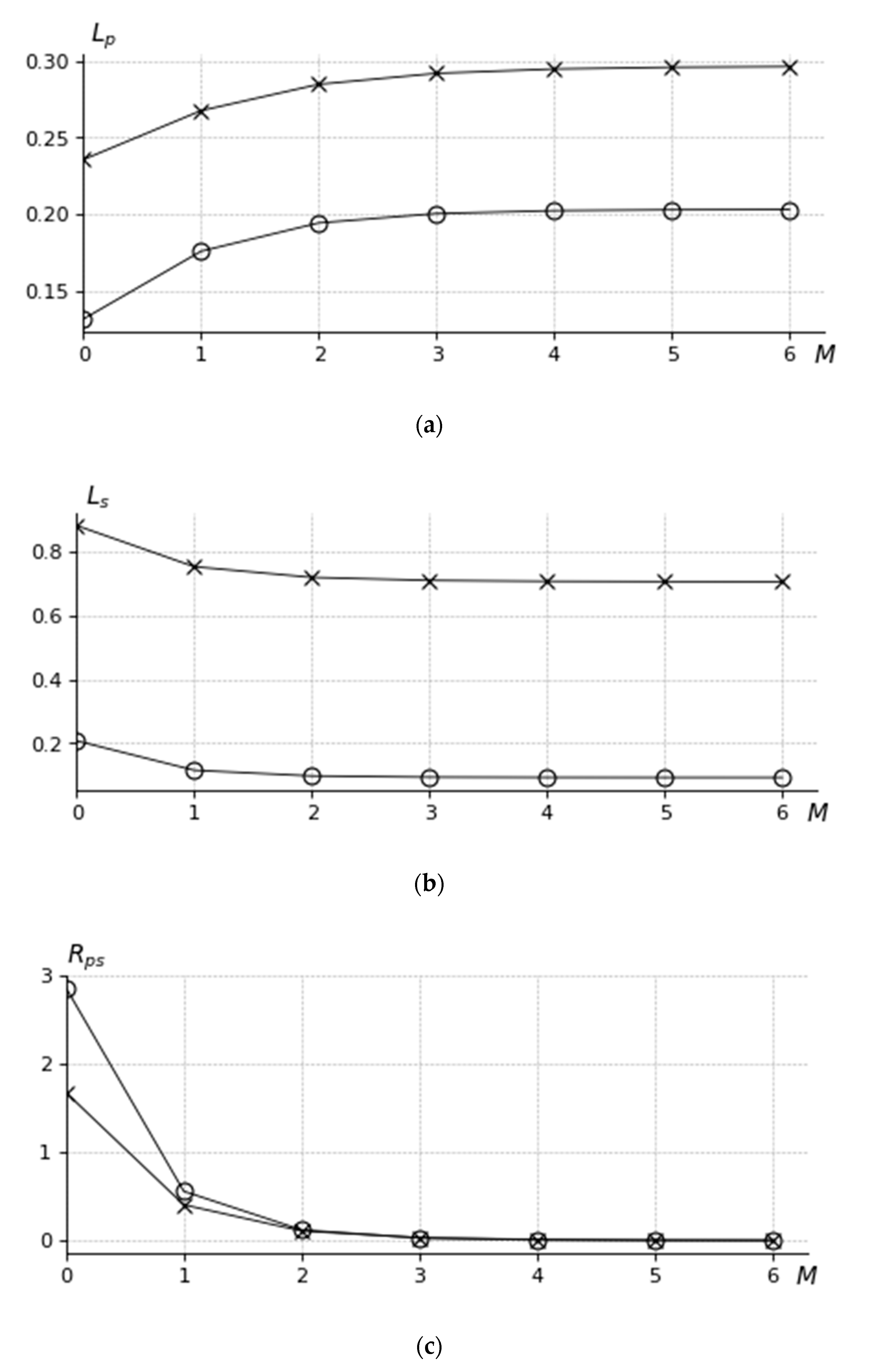
Behavior of performance measures relative to changes in the threshold parameter , with the above parameters of the MMPP flow and with , are shown in Figure 2. The function is non-decreasing (Figure 2a), which should be expected, since with an increase in the parameter the chances of initial calls joining their queue grows. For the same reason, the functions (Figure 2b) and (Figure 2c) are non-increasing.
Note that with increasing parameter the load of the S-server increases, and thus the chances of p-calls being served in this server decreases, and therefore, the number of such calls in front of the F-server increases (see Figure 2a); with increasing parameter the load of the S-server decreases, and thus, the number of such calls in the system decreases (see Figure 2b). The values of function Rps at different ratios of parameters and almost do not differ from each other (see Figure 2c).
In the numerical experiments discussed above, the autocorrelation of MMPP flow is close to zero. However, the great interest represents the estimation of accuracy of the developed approximate algorithm for the model with MMPP flow for which arrivals are strongly autocorrelated. For this reason, we consider a model where the infinitesimal matrix of a Markov chain with two states that control intensities of MMPP flow is defined as follows:
Let us say that the vector of intensities is equal to . Note that this MMPP flow has an autocorrelation of about 0.4 for the lag−1.
The parameters of the Bernoulli schemes were chosen as above, i.e., Results of numerical experiments for this case are given in Table 3. Comparative analysis of Table 3 with Table 1 and 2 shows that the accuracy of the developed approximate algorithm for such MMPP flow is slightly lower than for an MMPP flow with small autocorrelation coefficient. At the same time, it has a sufficiently high accuracy for practical applications.
5. Conclusions
The paper studies a model of a system with heterogeneous servers, MMPP flow, and instant feedback. After the completion of servicing in the high-speed server, primary calls according to the Bernoulli scheme either leave the system or immediately require re-servicing. Repeated (feedback) calls are served in a low-speed server, and after the service is completed, feedback calls can be repeated many times. If, at the time of the arrival of the primary call, the low-speed server is empty and the number of calls in the queue in front of the high-speed server exceeds a certain threshold value, then the incoming call, according to the Bernoulli scheme, is either sent for service to the low-speed server or joins its own queue. It is believed that primary and feedback calls can form queues of infinite or finite length.
For the case of infinite buffers, it is shown that the mathematical model of the system under study is a certain three-dimensional Markov chain with an infinite-dimensional state space. The ergodicity condition for the model is found and an approximate algorithm for calculating the steady-state probabilities of the corresponding Markov chain is developed. Using simulation experiments, the high accuracy of the developed algorithm has been shown.
A direction of further research might be indicated via investigation of similar model with MAP flow and PH(phase type) distribution of service time as well as the solving of the problem of finding the optimal value (in some sense) of the introduced threshold parameter.
Author Contributions
Conceptualization, A.M. and S.A.; methodology, A.M. and S.A.; software, S.A.; validation, S.A.; formal analysis, A.M., S.A. and J.S.; investigation, J.S., A.M.; writing—original draft preparation, A.M. and J.S.; writing—review and editing, A.M. and J.S.; supervision A.M.; project administration S.A. All authors have read and agreed to the published version of the manuscript.
Funding
The work of János Sztrik is supported by the EFOP-3.6.1-16-2016-00022 project. The project is co-financed by the European Union and the European Social Fund.
Acknowledgments
The authors are very grateful to the reviewers for their valuable comments and suggestions, which improved the quality and the presentation of the paper.
Conflicts of Interest
The authors declare no conflict of interest.
References
- Takacs, L. A single-server queue with feedback. Bell Syst. Tech. J. 1963, 42, 505–519. [Google Scholar] [CrossRef]
- Takacs, L. A queuing model with feedback. Oper. Res. 1977, 11, 345–354. [Google Scholar] [CrossRef]
- Melikov, A.Z.; Ponomarenko, L.A.; Rustamov, A.M. Methods for analysis of queuing models with instantaneous and delayed feedbacks. Commun. Comput. Inf. Sci. 2015, 564, 185–199. [Google Scholar]
- Sharma, S.K.; Kumar, R. A Markovian feedback queue with retention of reneged customers. Adv. Model. Optim. 2012, 14, 673–680. [Google Scholar]
- Sharma, S.K.; Kumar, R. A Markovian feedback queue with retention of reneged customers and balking. Adv. Model. Optim. 2012, 14, 681–688. [Google Scholar]
- Sharma, S.K.; Kumar, R. M/M/1 feedback queueing model with retention of reneged customers and balking. Am. J. Oper. Res. 2013, 3, 1–6. [Google Scholar]
- Sharma, S.K.; Kumar, R. A single-server Markovian feedback queuing system with discouraged arrivals and retention of reneged customers. Am. J. Oper. Res. 2013, 4, 35–39. [Google Scholar]
- Kumar, R.; Jain, N.K.; Som, B.K. Optimization of an M/M/1/N feedback queue with retention of reneged customers. Oper. Res. Decis. 2014, 24, 45–58. [Google Scholar]
- Santkumaran, A.; Thangaraj, V. A single server queue with impatient and feedback customers. Inf. Manag. Sci. 2000, 11, 71–79. [Google Scholar]
- Som, B.K.; Seth, S. M/M/c/N queuing system with encouraged arrivals, reneging, retention and feedback customers. Yugosl. J. Oper. Res. 2018, 28, 333–344. [Google Scholar] [CrossRef] [Green Version]
- Bouchentouf, A.A.; Kadi, M.; Rabhi, A. Analysis of two heterogeneous server queuing model with balking, reneging and feedback. Math. Sci. Appl. E Notes 2013, 2, 10–21. [Google Scholar]
- Dudin, A.N.; Kazimirsky, A.V.; Klimenok, V.I.; Breuer, L.; Krieger, U. The queuing model MAP/PH/1/N with feedback operating in a Markovian random environment. Austrian J. Stat. 2005, 34, 101–110. [Google Scholar]
- Krishnamoorthy, A.; Manjunath, A.S. On queues with priority determined by feedback. Calcutta Stat. Assoc. Bull. 2018, 70, 33–56. [Google Scholar] [CrossRef]
- Neuts, M.F. Matrix-Geometric Solutions in Stochastic Models: An Algorithmic Approach; John Hopkins University Press: Baltimore, MD, USA, 1981; p. 332. [Google Scholar]
- Melikov, A.Z.; Mehbaliyeva, E.V. Analysis and optimization of system with heterogeneous servers and jump priorities. J. Comput. Syst. Sci. Int. 2019, 58, 718–735. [Google Scholar] [CrossRef]
- Fisher, W.; Meier-Hellstern, K. The Markov-modulated Poisson process (MMPP) cookbook. Perform. Eval. 1992, 18, 149–171. [Google Scholar] [CrossRef]
- Melikov, A.Z.; Aliyeva, S.; Sztrik, J. Analysis of queuing system MMPP/M/K/K with delayed feedback. Mathematics 2019, 7, 1128. [Google Scholar] [CrossRef] [Green Version]
Figure 1.
Cosine similarity norm versus σ.

Figure 2.
Performance measures versus threshold parameter M; Lp vs M (a), Ls vs M (b), Rps vs M (c).
Figure 2.
Performance measures versus threshold parameter M; Lp vs M (a), Ls vs M (b), Rps vs M (c).


Table 1.
Accuracy of the developed algorithm for calculation of steady-state probabilities. Case of fixed values of intensities of Markov Modulated Poisson Process (MMPP) flow.
Table 1.
Accuracy of the developed algorithm for calculation of steady-state probabilities. Case of fixed values of intensities of Markov Modulated Poisson Process (MMPP) flow.
| Values of Norm (31) | ||
|---|---|---|
| (60, 45) | 1 | 0.9945 |
| 2 | 0.9940 | |
| 3 | 0.9914 | |
| (60, 50) | 1 | 0.9931 |
| 2 | 0.9948 | |
| 3 | 0.9927 | |
| (60, 55) | 1 | 0.9943 |
| 2 | 0.9951 | |
| 3 | 0.9954 | |
| (65, 45) | 1 | 0.9936 |
| 2 | 0.9944 | |
| 3 | 0.9936 | |
| (65, 50) | 1 | 0.9941 |
| 2 | 0.9958 | |
| 3 | 0.9953 | |
| (65, 55) | 1 | 0.9952 |
| 2 | 0.9949 | |
| 3 | 0.9958 | |
| (70, 45) | 1 | 0.9946 |
| 2 | 0.9955 | |
| 3 | 0.9950 | |
| (70, 50) | 1 | 0.9944 |
| 2 | 0.9968 | |
| 3 | 0.9960 | |
| (70, 55) | 1 | 0.9964 |
| 2 | 0.9970 | |
| 3 | 0.9960 |
Table 2.
Accuracy of the developed algorithm for calculation of steady-state probabilities. Case of varied values of intensities of MMPP flow.
Table 2.
Accuracy of the developed algorithm for calculation of steady-state probabilities. Case of varied values of intensities of MMPP flow.
| Values of Norm (31) | |||
|---|---|---|---|
| (10, 5, 3) | (60, 45) | 1 | 0.9979 |
| 2 | 0.9979 | ||
| 3 | 0.9973 | ||
| (65, 50) | 1 | 0.9983 | |
| 2 | 0.9984 | ||
| 3 | 0.9971 | ||
| (70, 55) | 1 | 0.9986 | |
| 2 | 0.9986 | ||
| 3 | 0.9986 | ||
| (15, 12, 17) | (60, 45) | 1 | 0.9924 |
| 2 | 0.9934 | ||
| 3 | 0.9914 | ||
| (65, 50) | 1 | 0.9953 | |
| 2 | 0.9949 | ||
| 3 | 0.9945 | ||
| (70, 55) | 1 | 0.9955 | |
| 2 | 0.9962 | ||
| 3 | 0.9964 | ||
| (20, 10, 5) | (60, 45) | 1 | 0.9892 |
| 2 | 0.9868 | ||
| 3 | 0.9867 | ||
| (65, 50) | 1 | 0.9903 | |
| 2 | 0.9904 | ||
| 3 | 0.9917 | ||
| (70, 55) | 1 | 0.9933 | |
| 2 | 0.9938 | ||
| 3 | 0.9936 |
Table 3.
Accuracy of the developed algorithm for calculation of steady-state probabilities. Case of autocorrelated arrivals of MMPP flow.
Table 3.
Accuracy of the developed algorithm for calculation of steady-state probabilities. Case of autocorrelated arrivals of MMPP flow.
| Values of the Norm (31) | |||
|---|---|---|---|
| 60 | 40 | 1 | 0.9908 |
| 40 | 3 | 0.7369 | |
| 45 | 2 | 0.9999 | |
| 50 | 1 | 0.9973 | |
| 55 | 2 | 0.9692 | |
| 55 | 3 | 0.7635 | |
| 65 | 40 | 3 | 0.8021 |
| 45 | 1 | 0.9749 | |
| 45 | 2 | 0.9917 | |
| 45 | 3 | 0.9839 | |
| 50 | 2 | 0.7357 | |
| 55 | 2 | 0.9699 | |
| 55 | 3 | 0.7803 | |
| 70 | 40 | 2 | 0.8742 |
| 45 | 2 | 0.9995 | |
| 45 | 3 | 0.9955 | |
| 50 | 1 | 0.8454 | |
| 50 | 2 | 0.9950 | |
| 50 | 3 | 0.9981 | |
| 55 | 2 | 0.9930 | |
| 75 | 40 | 2 | 0.9990 |
| 45 | 2 | 0.9543 | |
| 55 | 1 | 0.7905 | |
| 55 | 2 | 0.8041 | |
| 55 | 3 | 0.9967 |
Publisher’s Note: MDPI stays neutral with regard to jurisdictional claims in published maps and institutional affiliations. |
© 2020 by the authors. Licensee MDPI, Basel, Switzerland. This article is an open access article distributed under the terms and conditions of the Creative Commons Attribution (CC BY) license (http://creativecommons.org/licenses/by/4.0/).
Share and Cite
MDPI and ACS Style
Melikov, A.; Aliyeva, S.; Sztrik, J. Analysis of Instantaneous Feedback Queue with Heterogeneous Servers. Mathematics 2020, 8, 2186. https://doi.org/10.3390/math8122186
AMA Style
Melikov A, Aliyeva S, Sztrik J. Analysis of Instantaneous Feedback Queue with Heterogeneous Servers. Mathematics. 2020; 8(12):2186. https://doi.org/10.3390/math8122186
Chicago/Turabian StyleMelikov, Agassi, Sevinj Aliyeva, and János Sztrik. 2020. "Analysis of Instantaneous Feedback Queue with Heterogeneous Servers" Mathematics 8, no. 12: 2186. https://doi.org/10.3390/math8122186
Note that from the first issue of 2016, this journal uses article numbers instead of page numbers. See further details here.