Crossing Limit Cycles of Planar Piecewise Linear Hamiltonian Systems without Equilibrium Points

Abstract

In this paper, we study the existence of limit cycles of planar piecewise linear Hamiltonian systems without equilibrium points. Firstly, we prove that if these systems are separated by a parabola, they can have at most two crossing limit cycles, and if they are separated by a hyperbola or an ellipse, they can have at most three crossing limit cycles. Additionally, we prove that these upper bounds are reached. Secondly, we show that there is an example of two crossing limit cycles when these systems have four zones separated by three straight lines.

1. Introduction

The problem of the existence of limit cycles and mainly the problem of controlling their maximum number are two of the most difficult problems in the qualitative theory of differential systems in the plane. We solve these two problems for the class of discontinuous piecewise differential systems here considered.

We recall that a limit cycle is a periodic orbit of a differential system, which is isolated in the set of all periodic orbits of the system.

Limit cycles appear in a natural way in many applications. Thus, recently, the problem of the existence and the number of limit cycles has also been studied for discontinuous piecewise linear differential systems; this study goes back to Andronov et al. [1] and still has been given attention by researchers, mainly due to its simplicity and to its applications to a large number of phenomena, such as switches in electronic circuits, mechanical systems, etc.; see for instance [2,3,4], the books [5,6], and the hundreds of references quoted therein.

Lum and Chua [7] conjectured that a continuous planar piecewise linear system with two zones separated by a straight line can exhibit at most one limit cycle. Freire et al. [8] proved this conjecture in 1998. For the planar discontinuous piecewise linear systems, Han and Zhang [9] conjectured that these systems can have at most two crossing limit cycles when we separate them by a straight line, but Huan and Yang [10] gave a numerical example with three limit cycles; this result was proven analytically by Llibre and Ponce [11]. In 2015, Llibre et al. [12] proved that if we separate the planar discontinuous piecewise linear differential centers by a straight line, we cannot have any limit cycle. Recently, in the works [13,14,15,16], planar discontinuous linear differential centers separated by an algebraic curve, such as a conic, or a reducible and irreducible cubic, were studied, and it was proven that these differential systems can exhibit at most three crossing limit cycles having two intersection points with the conic of separation; the same result was proven if the curve of separation was a cubic.

In the literature, we find many papers studying piecewise smooth vector fields with two zones, and few papers for three and four zones.

In this paper, we consider planar piecewise linear Hamiltonian systems without equilibrium points.

Our first objective is to provide the exact maximum number of crossing limit cycles of planar discontinuous piecewise linear Hamiltonian systems without equilibrium points (PHS) and separated by a conic $\Sigma$. We follow the Filippov rules for defining the flow of the piecewise differential systems on a line of discontinuity; see [17].

We know that any conic takes nine canonical forms, but the four following forms: $x^2+1=0$, $x^2+y^2=0$, and $x^2+y^2+1=0$ do not separate the plane in connected regions, then we omit them. We do not study the crossing limit cycles separated by the conic $x^2-1=0$, because in [18], it was proven that PHS with three zones separated by two parallel straight lines have at most one crossing limit cycle.

The second objective of this paper is to study the crossing limit cycles of piecewise smooth differential systems such that in each piece, the differential system is linear, Hamiltonian, and without equilibrium points. Then, easy computations show that such differential system in each piece must have a vector field of the form:

$$X_i(x,y)=(-{\lambda }_i{b}_{i}x+b_{i}y+{\gamma }_i,-{\lambda }_i^2{b}_{i}x+{\lambda }_i{b}_{i}y+{\delta }_i),$$

${\delta }_i\ne {\lambda }_i{\gamma }_i$ and $b_i\ne 0$, with $i=1\dots 4$. Their corresponding Hamiltonian function is:

$$H_i(x,y)=(-{\lambda }_i^2{b}_i/2)x^2+{\lambda }_i{b}_{i}xy-(b_i/2)y^2+{\delta }_{i}x-{\gamma }_{i}y.$$

For more details, see [18].

1.1. Crossing Limit Cycles for Planar Piecewise Linear Hamiltonian Systems without Equilibrium Points Separated by a Conic

In this subsection, we give the upper bound of crossing limit cycles of PHS separated by a parabola, P: $y-x^2=0$, by a hyperbola H: $x^2-y^2-1=0$, or by an ellipse E: $x^2+y^2-1=0$.

We consider only the crossing limit cycles that intersect the conics in exactly two points, and for this reason, we will not study the crossing limit cycles separated by two intersecting straight lines $xy=0$.

Our first main result is the following.

Theorem 1.

The following statements hold.

(a) 

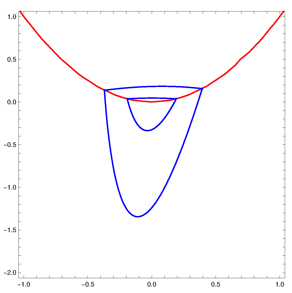
The maximum number of crossing limit cycles of PHS intersecting the parabolaPat two points is at most two, and this maximum is reached; see Figure 1.

(b) 

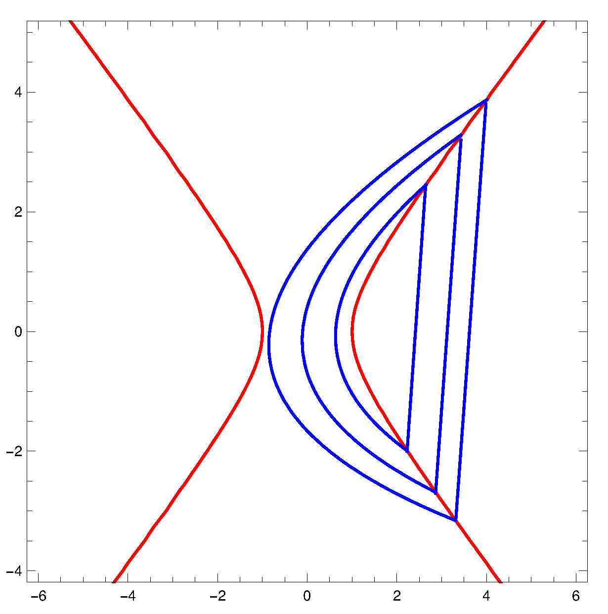
The maximum number of crossing limit cycles of PHS intersecting the hyperbolaHat two points is at most three, and this maximum is reached; see Figure 2.

(c) 

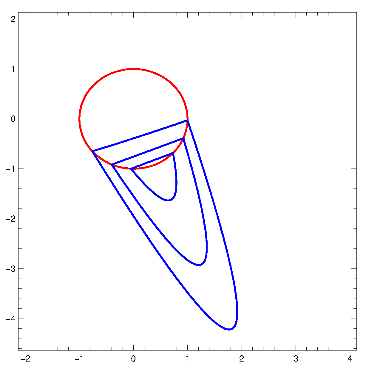
The maximum number of crossing limit cycles of PHS intersecting the ellipseEat two points is at most three, and this maximum is reached; see Figure 3.

The proof of Theorem 1 is given in Section 2.

1.2. Crossing Limit Cycles for Planar Piecewise Linear Hamiltonian Systems without Equilibrium Points with Four Zones

In this subsection, we study the existence of crossing limit cycles of the planar piecewise linear Hamiltonian systems without equilibrium points with four zones:

$$X(x,y)=\{\begin{array}{cc}{X}_1(x,y),\hfill & x\le -1,\hfill \\ X_2(x,y),\hfill & -1\le x\le 0,\hfill \\ X_3(x,y),\hfill & 0\le x\le 1,\hfill \\ X_4(x,y),\hfill & x\ge 1.\hfill \end{array}$$

(1)

satisfying the condition:

C. The vector fields $X_1$, $X_2$, $X_3$, and $X_4$ are linear and Hamiltonian without equilibrium points.

Our second results are the following.

Theorem 2.

Continuous planar piecewise Hamiltonian systems without equilibrium points with four zones satisfyingChave no crossing limit cycles.

Theorem 3.

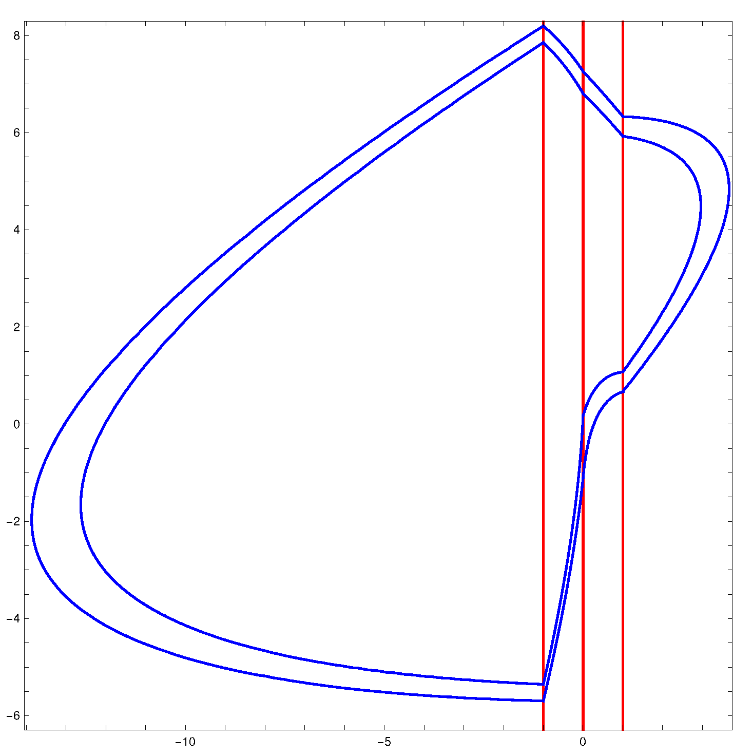
There are discontinuous planar piecewise Hamiltonian systems without equilibrium points with four zones satisfyingC, exhibiting exactly two crossing limit cycles; see Figure 4.

The proofs of Theorems 2 and 3 are given in Section 3.

2. Proof of Theorem 1

Proof of Statement (a) of Theorem 1.

In the region $R_1=\{(x,y):y-x^2\ge 0\}$, we consider the planar discontinuous piecewise linear Hamiltonian systems without equilibrium points:

$$\dot{x}=-{\lambda }_1{b}_{1}x+b_{1}y+{\gamma }_1,\dot{y}=-{\lambda }_1^2{b}_{1}x+{\lambda }_1{b}_{1}y+{\delta }_1,$$

(2)

with $b_1\ne 0$ and ${\delta }_1\ne {\lambda }_1{\gamma }_1$. The corresponding Hamiltonian function is:

$$H_1(x,y)=-({\lambda }_1^2{b}_1/2)x^2+{\lambda }_1{b}_{1}xy-(b_1/2)y^2+{\delta }_{1}x-{\gamma }_{1}y.$$

(3)

In the region $R_2=\{(x,y):y-x^2\le 0\}$, we consider:

$$\dot{x}=-{\lambda }_2{b}_{2}x+b_{2}y+{\gamma }_2,\dot{y}=-{\lambda }_2^2{b}_{2}x+{\lambda }_2{b}_{2}y+{\delta }_2,$$

(4)

with $b_2\ne 0$ and ${\delta }_2\ne {\lambda }_2{\gamma }_2$. The corresponding Hamiltonian function is:

$$H_2(x,y)=-({\lambda }_2^2{b}_2/2)x^2+{\lambda }_2{b}_{2}xy-(b_2/2)y^2+{\delta }_{2}x-{\gamma }_{2}y.$$

(5)

In order to have a crossing limit cycle that intersects the parabola $y-x^2=0$ at the points $(x_i,y_i)$ and $(x_k,y_k)$, these points must satisfy the following system:

$$\begin{array}{c}{H}_1(x_i,y_i)-H_1(x_k,y_k)=0,\hfill \\ H_2(x_i,y_i)-H_2(x_k,y_k)=0,\hfill \\ y_i-x_i^2=0,\hfill \\ y_k-x_k^2=0.\hfill \end{array}$$

(6)

We suppose that the two systems (2) and (4) have three crossing limit cycles. Then, System (6) must have three pairs of points as solutions, namely $p_i=(r_i,r_i^2)$ and $q_i=(s_i,s_i^2)$, with $i=1,2,3$. Due to the fact that these points satisfy System (6) and if we consider the points $p_1=(r_1,r_1^2)$ and $q_1=(s_1,s_1^2)$, solving the first two equations of (6) with respect to the parameters ${\gamma }_1$ and ${\gamma }_2$, we get:

$$\begin{array}{cc}{\gamma }_1=\hfill & {\displaystyle \frac{1}{2(r_1+s_1)}}(-r_1{r}_1^3-b_1{r}_1^2{s}_1-b_1{r}_1{s}_1^2-b_1{s}_1^3+2{\delta }_1+2b_1{r}_1^2{\lambda }_1+2b_1{r}_1{s}_1{\lambda }_1\hfill \\ & +2b_1{s}_1^2{\lambda }_1-b_1{r}_1{\lambda }_1^2-b_1{s}_1{\lambda }_1^2),\hfill \end{array}$$

and ${\gamma }_2$ has the same expression that ${\gamma }_1$ changes $(b_1,{\lambda }_1,{\delta }_1)$ by $(b_2,{\lambda }_2,{\delta }_2)$.

If the second points $p_2=(r_2,r_2^2)$ and $q_2=(s_2,s_2^2)$ satisfy System (6), then solving the first two equations of (6) with respect to the parameters ${\delta }_1$ and ${\delta }_2$, we get:

$$\begin{array}{cc}{\delta }_1=\hfill & {\displaystyle \frac{b_1}{2(r_1-r_2+s_1-s_2)}}(-r_1^3{r}_2-r_1{r}_2^3+r_1^2{r}_2{s}_1-r_2^3{s}_1+r_1{r}_2{s}_1^2+r_2{s}_1^3+r_1^3{s}_2\hfill \\ & -r_1{r}_2^2{s}_2+r_1^2{s}_1{s}_2-r_2^2{s}_1{s}_2+r_1{s}_1^2{s}_2+s_1^3{s}_2-r_1{r}_2{s}_2^2-r_2{s}_1{s}_2^2-r_1{s}_2^3-s_1{s}_2^3\hfill \\ & -2r_1^2{r}_2{\lambda }_1+2r_1{r}_2^2{\lambda }_1-2r_1{r}_2{s}_1{\lambda }_1+2r_2^2{s}_1{\lambda }_1-2r_2{s}_1^2{\lambda }_1-2r_1^2{s}_2{\lambda }_1+2r_1{r}_2{s}_2{\lambda }_1\hfill \\ & -2r_1{s}_1{s}_2{\lambda }_1+2r_2{s}_1{s}_2{\lambda }_1-2s_1^2{s}_2{\lambda }_1+2r_1{s}_2^2{\lambda }_1+2s_1{s}_2^2{\lambda }_1),\hfill \end{array}$$

and ${\delta }_2$ has the same expression that ${\delta }_1$ changes $(b_1,{\lambda }_1)$ by $(b_2,{\lambda }_2)$.

Finally, we suppose that the points $p_3=(r_3,r_3^2)$ and $q_3=(s_3,s_3^2)$ satisfy System (6), then the parameters ${\lambda }_1$ and ${\lambda }_2$ must be ${\lambda }_1=A/B$ where:

$$\begin{gathered} \begin{array}{cc}A=\hfill & r_1^3(r_2-r_3+s_2-s_3)+r_1^2{s}_1(r_2-r_3+s_2-s_3)+r_2^3(r_3-s_1+s_3)+r_2^2{s}_2(r_3-s_1\hfill \\ & +s_3)+r_1(-r_2^3+r_3^3-r_3{s}_1^2-r_2^2{s}_2+s_1^2{s}_2-s_2^3+r_2(s_1^2-s_2^2)+r_3^2{s}_3-s_1^2{s}_3+r_3{s}_3^2\hfill \\ & +s_3^3)+(s_1-s_2)(r_3^3+r_3^2{s}_3+(s_1-s_3)(s_2-s_3)(s_1+s_2+s_3)-r_3(s_1^2+s_1{s}_2+s_2^2\hfill \\ & -s_3^2\left)\right)-r_2(r_3^3-s_1^3+s_1{s}_2^2+r_3^2{s}_3-s_2^2{s}_3+s_3^3+r_3(-s_2^2+s_3^2)),\hfill \end{array} \\ \begin{array}{cc}B=\hfill & 2((s_1-s_2)(r_3^2+(s_1-s_3)(s_2-s_3)-r_3(s_1+s_2-s_3))+r_1^2(r_2-r_3+s_2-s_3)\hfill \\ & +r_2^2(r_3-s_1+s_3)+r_1(-r_2^2+r_3^2-r_3{s}_1+r_2(s_1-s_2)+s_1{s}_2-s_2^2+r_3{s}_3-s_1{s}_3\hfill \\ & +s_3^2)-r_2(r_3^2+r_3(-s_2+s_3)-(s_1-s_3)(s_1-s_2+s_3)).\hfill \end{array} \end{gathered}$$

${\lambda }_2$ has the same expression that ${\lambda }_1$ changes $b_1$ by $b_2$.

We replace ${\gamma }_1$, ${\lambda }_1$, and ${\delta }_1$ in the expression of $H_1(x,y)$ and ${\gamma }_2$, ${\lambda }_2$, and ${\delta }_2$ in the expression of $H_2(x,y)$, and we obtain $H_1(x,y)=H_2(x,y)$. Therefore, the piecewise linear differential system becomes a linear differential system, which does not have limit cycles. Therefore, the maximum number of crossing limit cycles in this case is two.

Example with two limit cycles. Consider the planar discontinuous piecewise linear Hamiltonian system without equilibrium points separated by the parabola P:

$$\dot{x}=5.5x-0.5y+3,\dot{y}=60.5x-5.5y+0.2;$$

in the region $R_1$, its corresponding Hamiltonian function is:

$$H_1(x,y)=30.25x^2-5.5xy+0.2x+0.25y^2-3y.$$

The second system is:

$$\dot{x}=0.2x-0.1y-0.778814,\dot{y}=0.4x-0.2y+0.00727332;$$

in the region $R_2$, its corresponding Hamiltonian function is:

$$H_2(x,y)=0.2x^2-0.2xy+0.00727332x+0.05y^2+0.778814y.$$

Now system (6) has the two solutions $({\alpha }_1,{\beta }_1,{\gamma }_1,{\delta }_1)=(0.191567..,0.0366978..,-0.191502..,0.036673..)$ and $({\alpha }_2,{\beta }_2,{\gamma }_2,{\delta }_2)=(0.395114..,0.156115..,-0.372692..,0.138899..)$. Which provide the two limit cycles shown in Figure 1. This completes the proof of Statement (a) of Theorem 1. □

Proof of Statement (b) of Theorem 1.

In the region $R_1=\{(x,y):x^2-y^2-1\ge 0\}$, we consider the PHS given in (2). Its corresponding Hamiltonian function is given by Equation (3).

In the region $R_2=\{(x,y):x^2-y^2-1\le 0\}$, we consider the PHS given in (2). Its corresponding Hamiltonian function is given by Equation (5).

In order to have a crossing limit cycle that intersects the hyperbola $x^2-y^2-1=0$ at the points $(x_i,y_i)$ and $(x_k,y_k)$, these points must satisfy the system:

$$\begin{array}{c}{H}_1(x_i,y_i)-H_1(x_k,y_k)=0,\hfill \\ H_2(x_i,y_i)-H_2(x_k,y_k)=0,\hfill \\ x_i^2-y_i^2=1,\hfill \\ x_k^2-y_k^2=1.\hfill \end{array}$$

(7)

We assume that the two systems (2) and (4) have four crossing limit cycles. Therefore, System (7) must have four pairs of points $p_i=(cosh{r}_i,sinh{r}_i)$ and $q_i=(cosh{s}_i,sinh{s}_i)$ for $i=1,2,3,4$ as solutions. Since these points satisfy System (7), we consider the points $p_1=(cosh{r}_1,sinh{r}_1)$ and $q_1=(cosh{s}_1,sinh{s}_1)$, and from (7), we obtain that the parameters ${\gamma }_1$ and ${\gamma }_2$ must be:

$$\begin{array}{cc}{\gamma }_1=\hfill & {\displaystyle \frac{1}{2(sinh{r}_1-sinh{s}_1)}}(2{\delta }_{1}cosh{r}_1-b_1{\lambda }_1^2{cosh}^2{r}_1+b_1{\lambda }_1^2{cosh}^2{s}_1-2cosh{s}_1({\delta }_1\hfill \\ & +b_1{\lambda }_{1}sinh{s}_1)+b_1(-{sinh}^2{r}_1+{\lambda }_{1}sinh\left(2r_1\right)+{sinh}^2{s}_1).\hfill \end{array}$$

If we change $(b_1,{\lambda }_1,{\delta }_1)$ by $(b_2,{\lambda }_2,{\delta }_2)$ in the expression of ${\gamma }_1$, we get the expression of ${\gamma }_2$.

We suppose that the second points $p_2=(cosh{r}_2,sinh{r}_2)$ and $q_2=(cosh{s}_2,sinh{s}_2)$ satisfy System (7), then the parameters ${\delta }_1$ and ${\delta }_2$ must be:

$$\begin{array}{cc}{\delta }_1=\hfill & {\displaystyle \frac{1}{4\left(cosh\left({\displaystyle \frac{r_1-2r_2+s_1}{2}}\right)-cosh\left({\displaystyle \frac{r_1+s_1-2s_2}{2}}\right)\right)}}(b_1\csc \mathrm{h}({\displaystyle \frac{r_1-s_1}{2}})(-{\lambda }_1^2{cosh}^2{r}_1\hfill \\ & sinh{r}_2+{\lambda }_1^2{cosh}^2{s}_{1}sinh{r}_2-{sinh}^2{r}_{1}sinh{r}_2+{\lambda }_{1}sinh\left(2r_1\right)sinh{r}_2+sinh{r}_1{sinh}^2{r}_2\hfill \\ & -{\lambda }_{1}sinh{r}_{1}sinh\left(2r_2\right)+{\lambda }_1^2{cosh}^2{r}_2(sinh{r}_1-sinh{s}_1)-{sinh}^2{r}_{2}sinh{s}_1+{\lambda }_{1}sinh\left(2r_2\right)\hfill \\ & sinh{s}_1+sinh{r}_2{sinh}^2{s}_1+{\lambda }_1^2{cosh}^2{s}_2(-sinh{r}_1+sinh{s}_1)-{\lambda }_{1}sinh{r}_{2}sinh\left(2s_1\right)\hfill \\ & +{\lambda }_1^2{cosh}^2{r}_{1}sinh{s}_2-{\lambda }_1^2{cosh}^2{s}_{1}sinh{s}_2+{sinh}^2{r}_{1}sinh{s}_2-{\lambda }_{1}sinh\left(2r_1\right)sinh{s}_2\hfill \\ & -{sinh}^2{s}_{1}sinh{s}_2+{\lambda }_{1}sinh\left(2s_1\right)sinh{s}_2-sinh{r}_1{sinh}^2{s}_2+sinh{s}_1{sinh}^2{s}_2\hfill \\ & +{\lambda }_1(sinh{r}_1-sinh{s}_1)sinh\left(2s_2\right)\left)\right).\hfill \end{array}$$

If we change $(b_1,{\lambda }_1)$ by $(b_2,{\lambda }_2)$ in the expression of ${\delta }_1$, we obtain ${\delta }_2$.

Now, we suppose that points $p_3=(cosh{r}_3,sinh{r}_3)$ and $q_3=(cosh{s}_3,sinh{s}_3)$ satisfy System (7), then we obtain two values of ${\lambda }_1$ (we name them ${\lambda }_1^{\left(1\right)}$ and ${\lambda }_1^{\left(2\right)}$) and two values of ${\lambda }_2$ (we name them ${\lambda }_2^{\left(1\right)}$ and ${\lambda }_2^{\left(2\right)}$). The first value of ${\lambda }_1$ is given by ${\lambda }_1^{\left(1\right)}=(A-(1/2)\sqrt{B})/C$ and ${\lambda }_1^{\left(2\right)}=(A+(1/2)\sqrt{B})/C$, where:

$$\begin{array}{cc}A=\hfill & -sinh\left({\displaystyle \frac{r_1-r_2-r_3+s_1-s_2-3s_3}{2}}\right)+sinh\left({\displaystyle \frac{r_1-r_2-r_3+s_1-3s_2-s_3}{2}}\right)\hfill \\ & -sinh\left({\displaystyle \frac{r_1-r_2-3r_3+s_1-s_2-s_3}{2}}\right)+sinh\left({\displaystyle \frac{r_1-3r_2-r_3+s_1-s_2-s_3}{2}}\right)\hfill \\ & -sinh\left({\displaystyle \frac{3r_1+r_2-r_3+s_1+s_2-s_3}{2}}\right)+sinh\left({\displaystyle \frac{r_1+3r_2-r_3+s_1+s_2-s_3}{2}}\right)\hfill \\ & -sinh\left({\displaystyle \frac{r_1+r_2-r_3+3s_1+s_2-s_3}{2}}\right)+sinh\left({\displaystyle \frac{r_1+r_2-r_3+s_1+3s_2-s_3}{2}}\right)\hfill \\ & +sinh\left({\displaystyle \frac{3r_1-r_2+r_3+s_1-s_2+s_3}{2}}\right)-sinh\left({\displaystyle \frac{r_1-r_2+3r_3+s_1-s_2+s_3}{2}}\right)\hfill \\ & +sinh\left({\displaystyle \frac{r_1-r_2+r_3+3s_1-s_2+s_3}{2}}\right)-sinh\left({\displaystyle \frac{r_1-r_2+r_3+s_1-s_2+3s_3}{2}}\right),\hfill \end{array}$$

$$\begin{array}{cc}B=\hfill & -4(cosh\left({\displaystyle \frac{r_1-r_2-r_3+s_1-s_2-3s_3}{2}}\right)-cosh\left({\displaystyle \frac{r_1-r_2-r_3+s_1-3s_2-s_3}{2}}\right)\hfill \\ & +cosh\left({\displaystyle \frac{r_1-r_2-3r_3+s_1-s_2-s_3}{2}}\right)-cosh\left({\displaystyle \frac{r_1-3r_2-r_3+s_1-s_2-s_3}{2}}\right)\hfill \\ & -cosh\left({\displaystyle \frac{3r_1+r_2-r_3+s_1+s_2-s_3}{2}}\right)+cosh\left({\displaystyle \frac{r_1+3r_2-r_3+s_1+s_2-s_3}{2}}\right)\hfill \\ & -cosh\left({\displaystyle \frac{r_1+r_2-r_3+3s_1+s_2-s_3}{2}}\right)+cosh\left({\displaystyle \frac{r_1+r_2-r_3+s_1+3s_2-s_3}{2}}\right)\hfill \\ & +cosh\left({\displaystyle \frac{3r_1-r_2+r_3+s_1-s_2+s_3}{2}}\right)-cosh\left({\displaystyle \frac{r_1-r_2+3r_3+s_1-s_2+s_3}{2}}\right)\hfill \\ & +cosh\left({\displaystyle \frac{r_1-r_2+r_3+3s_1-s_2+s_3}{2}}\right)-{cosh}^2\left({\displaystyle \frac{r_1-r_2+r_3+s_1-s_2+3s_3}{2}}\right))\hfill \\ & +4(sinh\left({\displaystyle \frac{r_1-r_2-r_3+s_1-s_2-3s_3}{2}}\right)-sinh\left({\displaystyle \frac{r_1-r_2-r_3+s_1-3s_2-s_3}{2}}\right)\hfill \\ & +sinh\left({\displaystyle \frac{r_1-r_2-3r_3+s_1-s_2-s_3}{2}}\right)-sinh\left({\displaystyle \frac{r_1-3r_2-r_3+s_1-s_2-s_3}{2}}\right)\hfill \\ & +sinh\left({\displaystyle \frac{3r_1+r_2-r_3+s_1+s_2-s_3}{2}}\right)-sinh\left({\displaystyle \frac{r_1+3r_2-r_3+s_1+s_2-s_3}{2}}\right)\hfill \\ & +sinh\left({\displaystyle \frac{r_1+r_2-r_3+3s_1+s_2-s_3}{2}}\right)-sinh\left({\displaystyle \frac{r_1+r_2-r_3+s_1+3s_2-s_3}{2}}\right)\hfill \\ & -sinh\left({\displaystyle \frac{3r_1-r_2+r_3+s_1-s_2+s_3}{2}}\right)+sinh\left({\displaystyle \frac{r_1-r_2+3r_3+s_1-s_2+s_3}{2}}\right)\hfill \\ & -sinh\left({\displaystyle \frac{r_1-r_2+r_3+3s_1-s_2+s_3}{2}}\right)+{sinh}^2\left({\displaystyle \frac{r_1-r_2+r_3+s_1-s_2+3s_3}{2}}\right)),\hfill \end{array}$$

and the expression of C is:

$$\begin{array}{cc}C=\hfill & cosh\left({\displaystyle \frac{r_1-r_2-r_3+s_1-s_2-3s_3}{2}}\right)-cosh\left({\displaystyle \frac{r_1-r_2-r_3+s_1-3s_2-s_3}{2}}\right)\hfill \\ & +cosh\left({\displaystyle \frac{r_1-r_2-3r_3+s_1-s_2-s_3}{2}}\right)-cosh\left({\displaystyle \frac{r_1-3r_2-r_3+s_1-s_2-s_3}{2}}\right)\hfill \\ & -cosh\left({\displaystyle \frac{3r_1+r_2-r_3+s_1+s_2-s_3}{2}}\right)+cosh\left({\displaystyle \frac{r_1+3r_2-r_3+s_1+s_2-s_3}{2}}\right)\hfill \\ & -cosh\left({\displaystyle \frac{r_1+r_2-r_3+3s_1+s_2-s_3}{2}}\right)+cosh\left({\displaystyle \frac{r_1+r_2-r_3+s_1+3s_2-s_3}{2}}\right)\hfill \\ & +cosh\left({\displaystyle \frac{3r_1-r_2+r_3+s_1-s_2+s_3}{2}}\right)-cosh\left({\displaystyle \frac{r_1-r_2+3r_3+s_1-s_2+s_3}{2}}\right)\hfill \\ & +cosh\left({\displaystyle \frac{r_1-r_2+r_3+3s_1-s_2+s_3}{2}}\right)-cosh\left({\displaystyle \frac{r_1-r_2+r_3+s_1-s_2+3s_3}{2}}\right).\hfill \end{array}$$

We get the expression of ${\lambda }_2^{\left(1\right)}$ and ${\lambda }_2^{\left(2\right)}$ by changing $b_1$ by $b_2$ in the expression of ${\lambda }_1^{\left(1\right)}$ and ${\lambda }_1^{\left(2\right)}$, respectively.

We replace ${\gamma }_1$, ${\delta }_1$, and ${\lambda }_1^{\left(i\right)}$ in the expression of $H_1(x,y)$ and ${\gamma }_2$, ${\delta }_2$, and ${\lambda }_2^{\left(i\right)}$ in the expression of $H_2(x,y)$, and we obtain $H_1(x,y)=H_2(x,y)$, for $i=1,2$. Hence, in these cases, the piecewise linear differential system becomes a linear differential system, which does not have limit cycles. Therefore, the maximum number of crossing limit cycles in this case is two.

Now, we consider either ${\lambda }_1^{\left(2\right)}$ and ${\lambda }_2^{\left(1\right)}$ or ${\lambda }_1^{\left(1\right)}$ and ${\lambda }_2^{\left(2\right)}$, by replacing the expressions of ${\gamma }_1$, ${\delta }_1$, and ${\lambda }_1^{\left(2\right)}$ (resp. ${\lambda }_1^{\left(1\right)}$) in the expression of $H_1(x,y)$ and ${\gamma }_2$, ${\delta }_2$, and ${\lambda }_2^{\left(1\right)}$ (resp. ${\lambda }_2^{\left(2\right)}$) in the expression of $H_2(x,y)$; we have $H_1(x,y)\ne H_2(x,y)$.

Then, we assume that points $p_4=(cosh{r}_4,sinh{r}_4)$ and $q_4=(cosh{s}_4,sinh{s}_4)$ satisfy System (7), then we obtain $b_1=0$ and $b_2=0$. This is a contradiction because by the assumptions, they are not zero. Then, we proved that the maximum number of crossing limit cycles for PHS separated by a hyperbola is at most three.

Example with three limit cycles. We consider a PHS separated by the hyperbola H:

$$\dot{x}=-0.14..x+1.4y+\frac{1}{5},\dot{y}=-0.014..x+0.14y+1.9,$$

(8)

in the region $R_1=\{(x,y):x^2-y^2-1\le 0\}$. It has the Hamiltonian function:

$$H_1(x,y)=-0.007..x^2+0.14xy+1.9x-0.7y^2-\frac{y}{5}.$$

Now, we consider the second PHS:

$$\dot{x}=5x-\frac{y}{2}-7.14286..,\dot{y}=50x-5y-67.8571..,$$

(9)

in the region $R_2=\{(x,y):x^2-y^2-1\ge 0,x>1\}$. This differential system has the Hamiltonian function:

$$H_2(x,y)=25x^2-5xy-67.8571..x+\frac{y^2}{4}+7.14286..y.$$

The PHS (8)–(9) has exactly three crossing limit cycles, because the system of equations:

$$\begin{array}{c}{H}_1(\alpha ,\beta )-H_1(\gamma ,\delta )=0,\hfill \\ H_2(\alpha ,\beta )-H_2(\gamma ,\delta )=0,\hfill \\ {\alpha }^2-{\beta }^2-1=0,\hfill \\ {\gamma }^2-{\delta }^2-1=0,\hfill \end{array}$$

(10)

has three real solutions $({\alpha }_1,{\beta }_1,{\gamma }_1,{\delta }_1)=(3.99376\dots ,3.86653\dots ,3.31341\dots ,-3.1589..)$, $({\alpha }_2,{\beta }_2,{\gamma }_2,{\delta }_2)=(3.43842\dots ,3.28979\dots ,2.86513\dots ,-2.68496..)$, and $({\alpha }_3,{\beta }_3,{\gamma }_3,{\delta }_3)=(2.64219\dots ,2.44565\dots ,2.2285\dots ,-1.99154\dots )$; see Figure 2. □

Proof of Statement (c) of Theorem 1.

We consider the PHS given in (2) in the region $R_1=\{(x,y):x^2+y^2-1\ge 0\}$, with its corresponding Hamiltonian function (3).

We consider the PHS given in (2) in the region $R_2=\{(x,y):x^2+y^2-1\le 0\}$, with its corresponding Hamiltonian function (5).

In order that Systems (2) and (4) have crossing limit cycles intersecting the ellipse $x^2+x^2-1=0$ at the points $(x_i,y_i)$ and $(x_k,y_k)$, they must satisfy the system:

$$\begin{array}{c}{H}_1(x_i,y_i)-H_1(x_k,y_k)=0,\hfill \\ H_2(x_i,y_i)-H_2(x_k,y_k)=0,\hfill \\ x_i^2+y_i^2=1,\hfill \\ x_k^2+y_k^2=1.\hfill \end{array}$$

(11)

We suppose that Systems (2) and (4) have four crossing limit cycles. Therefore, System (11) must have four pairs of points $p_i=(cos{r}_i,sin{r}_i)$ and $q_i=(cos{s}_i,sin{s}_i)$ for $i=1,2,3,4$ as solutions. Therefore, if we consider the points $p_1=(cos{r}_1,sin{r}_1)$ and $q_1=(cos{s}_1,sin{s}_1)$, from (11), we obtain that the parameters ${\gamma }_1$ and ${\gamma }_2$ must be:

$$\begin{array}{cc}{\gamma }_1=\hfill & {\displaystyle \frac{1}{4(sin{r}_1-sin{s}_1)}}(4{\delta }_{1}cos{r}_1+b_{1}cos\left(2r_1\right)-b_1{\lambda }_1^{2}cos\left(2r_1\right)-4{\delta }_{1}cos{s}_1-b_{1}cos\left(2s_1\right)\hfill \\ & +b_1{\lambda }_1^{2}cos\left(2s_1\right)+2b_1{\lambda }_{1}sin\left(2r_1\right)-2b_1{\lambda }_{1}sin\left(2s_1\right)).\hfill \end{array}$$

If we change $(b_1,{\lambda }_1,{\delta }_1)$ by $(b_2,{\lambda }_2,{\delta }_2)$ in the expression of ${\gamma }_1$, we get the expression of ${\gamma }_2$.

Now, if the second points $p_2=(cos{r}_2,sin{r}_2)$ and $q_2=(cos{s}_2,sin{s}_2)$ satisfy System (11), then the parameters ${\delta }_1$ and ${\delta }_2$ take the values:

$$\begin{array}{cc}{\delta }_1=\hfill & {\displaystyle \frac{r_{1}cos((r_1+s_1)/2)csc((r_2-s_2)/2)csc((r_1-r_2+s_1-s_2)/2)}{4\left(sin{r}_1-sin{s}_1\right)}}({\lambda }_1^2{cos}^2{r}_{2}sin{r}_1\hfill \\ & -{\lambda }_1^2{cos}^2{s}_{2}sin{r}_1-2{\lambda }_{1}cos{r}_{2}sin{r}_{1}sin{r}_2+sin{r}_1{sin}^2{r}_2+2{\lambda }_{1}cos(r_1+s_1)\hfill \\ & sin{r}_{2}sin(r_1-s_1)-{\lambda }_1^2{cos}^2{r}_{2}sin{s}_1+{\lambda }_1^2{cos}^2{s}_{2}sin{s}_1+2{\lambda }_{1}cos{r}_{2}sin{r}_{2}sin{s}_1\hfill \\ & -{sin}^2{r}_{2}sin{s}_1-sin{r}_{2}sin(r_1-s_1)sin(r_1+s_1)+{\lambda }_1^{2}sin{r}_{2}sin(r_1-s_1)sin(r_1+s_1)\hfill \\ & -2{\lambda }_{1}cos(r_1+s_1)sin(r_1-s_1)sin{s}_2+sin(r_1-s_1)sin(r_1+s_1)sin{s}_2-{\lambda }_1^2\hfill \\ & sin(r_1-s_1)sin(r_1+s_1)sin{s}_2-sin{r}_1{sin}^2{s}_2+sin{s}_1{sin}^2{s}_2+{\lambda }_{1}sin{r}_{1}sin\left(2s_2\right)\hfill \\ & -{\lambda }_{1}sin{s}_{1}sin\left(2s_2\right)).\hfill \end{array}$$

If we change $(b_1,{\lambda }_1)$ by $(b_2,{\lambda }_2)$ in the expression of ${\delta }_1$, we obtain ${\delta }_2$.

If we assume that the points $p_3=(cos{r}_3,sin{r}_3)$ and $q_3=(cos{s}_3,sin{s}_3)$ satisfy System (11), then we obtain two values of ${\lambda }_1$, namely ${\lambda }_1^{\left(1\right)}$ and ${\lambda }_1^{\left(2\right)}$, and two values of ${\lambda }_2$, namely ${\lambda }_2^{\left(1\right)}$ and ${\lambda }_2^{\left(2\right)}$, such that ${\lambda }_1^{\left(1\right)}=(A+\sqrt{B})/C$ and ${\lambda }_1^{\left(2\right)}=(A-\sqrt{B})/C$, where:

$$\begin{array}{cc}A=\hfill & -sin\left({\displaystyle \frac{r_1-r_2-r_3+s_1-s_2-3s_3}{2}}\right)+sin\left({\displaystyle \frac{r_1-r_2-r_3+s_1-3s_2-s_3}{2}}\right)\hfill \\ & -sin\left({\displaystyle \frac{r_1-r_2-3r_3+s_1-s_2-s_3}{2}}\right)+sin\left({\displaystyle \frac{r_1-3r_2-r_3+s_1-s_2-s_3}{2}}\right)\hfill \\ & -sin\left({\displaystyle \frac{3r_1+r_2-r_3+s_1+s_2-s_3}{2}}\right)+sin\left({\displaystyle \frac{r_1+3r_2-r_3+s_1+s_2-s_3}{2}}\right)\hfill \\ & -sin\left({\displaystyle \frac{r_1+r_2-r_3+3s_1+s_2-s_3}{2}}\right)+sin\left({\displaystyle \frac{r_1+r_2-r_3+s_1+3s_2-s_3}{2}}\right)\hfill \\ & +sin\left({\displaystyle \frac{3r_1-r_2+r_3+s_1-s_2+s_3}{2}}\right)-sin\left({\displaystyle \frac{r_1-r_2+3r_3+s_1-s_2+s_3}{2}}\right)\hfill \\ & +sin\left({\displaystyle \frac{r_1-r_2+r_3+3s_1-s_2+s_3}{2}}\right)-sin\left({\displaystyle \frac{r_1-r_2+r_3+s_1-s_2+3s_3}{2}}\right),\hfill \end{array}$$

$$\begin{array}{cc}B=\hfill & cos\left({\displaystyle \frac{r_1-r_2-r_3+s_1-s_2-3s_3}{2}}\right)-cos\left({\displaystyle \frac{r_1-r_2-r_3+s_1-3s_2-s_3}{2}}\right)\hfill \\ & +cos\left({\displaystyle \frac{r_1-r_2-3r_3+s_1-s_2-s_3}{2}}\right)-cos\left({\displaystyle \frac{r_1-3r_2-r_3+s_1-s_2-s_3}{2}}\right)\hfill \\ & -cos\left({\displaystyle \frac{3r_1+r_2-r_3+s_1+s_2-s_3}{2}}\right)+cos\left({\displaystyle \frac{r_1+3r_2-r_3+s_1+s_2-s_3}{2}}\right)\hfill \\ & -cos\left({\displaystyle \frac{r_1+r_2-r_3+3s_1+s_2-s_3}{2}}\right)+cos\left({\displaystyle \frac{r_1+r_2-r_3+s_1+3s_2-s_3}{2}}\right)\hfill \\ & +cos\left({\displaystyle \frac{3r_1-r_2+r_3+s_1-s_2+s_3}{2}}\right)-cos\left({\displaystyle \frac{r_1-r_2+3r_3+s_1-s_2+s_3}{2}}\right)\hfill \\ & +cos\left({\displaystyle \frac{r_1-r_2+r_3+3s_1-s_2+s_3}{2}}\right)-{cos}^2\left({\displaystyle \frac{r_1-r_2+r_3+s_1-s_2+3s_3}{2}}\right)\hfill \\ & +(sin\left({\displaystyle \frac{r_1-r_2-r_3+s_1-s_2-3s_3}{2}}\right)-sin\left({\displaystyle \frac{r_1-r_2-r_3+s_1-3s_2-s_3}{2}}\right)\hfill \\ & +sin\left({\displaystyle \frac{r_1-r_2-3r_3+s_1-s_2-s_3}{2}}\right)-sin\left({\displaystyle \frac{r_1-3r_2-r_3+s_1-s_2-s_3}{2}}\right)\hfill \\ & +sin\left({\displaystyle \frac{3r_1+r_2-r_3+s_1+s_2-s_3}{2}}\right)-sin\left({\displaystyle \frac{r_1+3r_2-r_3+s_1+s_2-s_3}{2}}\right)\hfill \\ & +sin\left({\displaystyle \frac{r_1+r_2-r_3+3s_1+s_2-s_3}{2}}\right)-sin\left({\displaystyle \frac{r_1+r_2-r_3+s_1+3s_2-s_3}{2}}\right)\hfill \\ & -sin\left({\displaystyle \frac{3r_1-r_2+r_3+s_1-s_2+s_3}{2}}\right)+sin\left({\displaystyle \frac{r_1-r_2+3r_3+s_1-s_2+s_3}{2}}\right)\hfill \\ & -sin\left({\displaystyle \frac{r_1-r_2+r_3+3s_1-s_2+s_3}{2}}\right)+{sin}^2\left({\displaystyle \frac{r_1-r_2+r_3+s_1-s_2+3s_3}{2}}\right),\hfill \end{array}$$

and the expression of C is:

$$\begin{array}{cc}C=\hfill & cos\left({\displaystyle \frac{r_1-r_2-r_3+s_1-s_2-3s_3}{2}}\right)-cos\left({\displaystyle \frac{r_1-r_2-r_3+s_1-3s_2-s_3}{2}}\right)\hfill \\ & +cos\left({\displaystyle \frac{r_1-r_2-3r_3+s_1-s_2-s_3}{2}}\right)-cos\left({\displaystyle \frac{r_1-3r_2-r_3+s_1-s_2-s_3}{2}}\right)\hfill \\ & -cos\left({\displaystyle \frac{3r_1+r_2-r_3+s_1+s_2-s_3}{2}}\right)+cos\left({\displaystyle \frac{r_1+3r_2-r_3+s_1+s_2-s_3}{2}}\right)\hfill \\ & -cos\left({\displaystyle \frac{r_1+r_2-r_3+3s_1+s_2-s_3}{2}}\right)+cos\left({\displaystyle \frac{r_1+r_2-r_3+s_1+3s_2-s_3}{2}}\right)\hfill \\ & +cos\left({\displaystyle \frac{3r_1-r_2+r_3+s_1-s_2+s_3}{2}}\right)-cos\left({\displaystyle \frac{r_1-r_2+3r_3+s_1-s_2+s_3}{2}}\right)\hfill \\ & +cos\left({\displaystyle \frac{r_1-r_2+r_3+3s_1-s_2+s_3}{2}}\right)-cos\left({\displaystyle \frac{r_1-r_2+r_3+s_1-s_2+3s_3}{2}}\right).\hfill \end{array}$$

The expressions of ${\lambda }_2^{\left(1\right)}$ and ${\lambda }_2^{\left(2\right)}$ are the same as the expressions of ${\lambda }_1^{\left(1\right)}$ and ${\lambda }_1^{\left(2\right)}$, respectively, if we change $b_1$ by $b_2$.

We replace ${\gamma }_1$, ${\delta }_1$, and ${\lambda }_1^{\left(i\right)}$ in the expression of $H_1(x,y)$ and ${\gamma }_2$, ${\delta }_2$ and ${\lambda }_2^{\left(i\right)}$ in the expression of $H_2(x,y)$, and we obtain $H_1(x,y)=H_2(x,y)$ for $i=1,2$. Therefore, the maximum number of crossing limit cycles in these cases is two.

Now, we consider either ${\lambda }_1^{\left(2\right)}$ and ${\lambda }_2^{\left(1\right)}$ or ${\lambda }_1^{\left(1\right)}$ and ${\lambda }_2^{\left(2\right)}$, by replacing the expressions of ${\gamma }_1$, ${\delta }_1$, and ${\lambda }_1^{\left(2\right)}$ (resp. ${\lambda }_1^{\left(1\right)}$) in the expression of $H_1(x,y)$ and ${\gamma }_2$, ${\delta }_2$ and ${\lambda }_2^{\left(1\right)}$ (resp. ${\lambda }_2^{\left(2\right)}$) in the expression of $H_2(x,y)$, and we get two different expressions of the Hamiltonian functions $H_1(x,y)$ and $H_2(x,y)$.

Then, we assume that points $p_4=(cos{r}_4,sin{r}_4)$ and $q_4=(cos{s}_4,sin{s}_4)$ satisfy System (11), and by solving this system, we obtain $b_1=0$ and $b_2=0$, which is a contradiction. Then, we proved that the maximum number of crossing limit cycles for PHS separated by an ellipse is at most three.

Example with three limit cycles. In the region $R_1=\{(x,y):x^2+y^2-1\ge 0\}$, we consider the linear PHS:

$$\dot{x}=2.53..x+1.1..y-0.6..,\dot{y}=-5.819..x-2.53..y-0.4..;$$

(12)

its Hamiltonian function is:

$$H_1(x,y)=-2.9095..x^2-2.53..xy-0.4..x-0.55..y^2+0...6y.$$

In the region $R_2=\{(x,y):x^2+y^2-1\le 0\}$, we consider the linear PHS:

$$\dot{x}=-0.308696..x+0.71..y+0.0732085..,\dot{y}=-0.134216..x+0.308696..y+0.0488056..$$

(13)

Its Hamiltonian function is:

$$H_2(x,y)=-0.0671078..x^2+0.308696..xy+0.0488056..x-0.355..y^2-0.0732085..y.$$

The linear PHS (12)–(13) has exactly three crossing limit cycles, because the system of equations:

$$\begin{array}{c}{H}_1(\alpha ,\beta )-H_1(\gamma ,\delta )=0,\hfill \\ H_2(\alpha ,\beta )-H_2(\gamma ,\delta )=0,\hfill \\ {\alpha }^2+{\beta }^2-1=0,\hfill \\ {\gamma }^2+{\delta }^2-1=0,\hfill \end{array}$$

(14)

has three real solutions $({\alpha }_1,{\beta }_1,{\gamma }_1,{\delta }_1)=(-0.0450412\dots ,-0.998985\dots ,0.730814\dots ,-0.682576\dots )$, $({\alpha }_2,{\beta }_2,{\gamma }_2,{\delta }_2)=(-0.40163\dots ,-0.915802\dots ,0.92153\dots ,-0.388307\dots )$, and $({\alpha }_3,{\beta }_3,{\gamma }_3,{\delta }_3)=(-0.760814..,-0.64897..,0.99956..,-0.0296781..)$ □

We mention that the proof of Theorem 1 can be also analyzed using the results of [19].

3. Proof of Theorems 2 and 3

Proof of Theorem 2.

Consider a continuous linear Hamiltonian differential system separated by the straight lines $x=-1$, $x=0$, and $x=1$. According to the continuity of the vector field X, we obtain:

$$X_1(-1,y)=X_2(-1,y),X_2(0,y)=X_3(0,y)and{X}_3(1,y)=X_4(0,y),\forall y\in \mathbb{R},$$

which imply that:

$$\begin{array}{c}{b}_1=b_2=b_3=b_4=b,\hfill \\ {\delta }_1={\delta }_2={\delta }_3={\delta }_4=\delta ,\hfill \\ {\gamma }_1={\gamma }_2={\gamma }_3={\gamma }_4=\gamma ,\hfill \\ {\lambda }_1={\lambda }_2={\lambda }_3={\lambda }_4=\lambda .\hfill \end{array}$$

Therefore, from System (1), the piecewise vector field becomes the vector field:

$$X(x,y)=(-\lambda bx+by+\gamma ,-{\lambda }^{2}bx+\lambda by+\delta ),\delta \ne \lambda \gamma ,b\ne 0.$$

Since this linear differential system has no equilibrium point, it has no periodic orbits, then no limit cycles. This completes the proof of Theorem 2. □

Proof of Theorem 3.

If the PHS with four zones have crossing limit cycles, then there are crossing points $(-1,y_0)$, $(-1,y_5)$, $(0,y_1)$, $(0,y_4)$, and $(1,y_2)$, $(1,y_3)$ satisfying:

$$\begin{array}{c}{H}_1(-1,y_0)=H_1(-1,y_5),\hfill \\ H_2(-1,y_0)=H_2(0,y_1),\hfill \\ H_2(-1,y_5)=H_2(0,y_4),\hfill \\ H_3((0,y_1)=H_3(1,y_2),\hfill \\ H_3((0,y_4)=H_3(1,y_3),\hfill \\ H_4((1,y_2)=H_4(1,y_3),\hfill \end{array}$$

(15)

or equivalently:

$$\begin{array}{ccc}\hfill (y_0-y_5)(2b_1{\lambda }_1+b_1{y}_0+b_1{y}_5+2{\gamma }_1)& =& \hfill 0,\end{array}$$

(16)

$$\begin{array}{ccc}\hfill -b_2{\lambda }_2^2-b_2{y}_0^2-2b_2{\lambda }_2{y}_0+b_2{y}_1^2-2{\delta }_2-2{\gamma }_2{y}_0+2{\gamma }_2{y}_1& =& \hfill 0,\end{array}$$

(17)

$$\begin{array}{ccc}\hfill -b_2{\lambda }_2^2+b_2{y}_4^2-b_2{y}_5^2-2b_2{\lambda }_2{y}_5-2{\delta }_2+2{\gamma }_2{y}_4-2{\gamma }_2{y}_5& =& \hfill 0,\end{array}$$

(18)

$$\begin{array}{ccc}\hfill b_3{\lambda }_3^2-b_3{y}_1^2+b_3{y}_2^2-2b_3{\lambda }_3{y}_2-2{\delta }_3-2{\gamma }_3{y}_1+2{\gamma }_3{y}_2& =& \hfill 0,\end{array}$$

(19)

$$\begin{array}{ccc}\hfill b_3{\lambda }_3^2+b_3{y}_3^2-2b_3{\lambda }_3{y}_3-b_3{y}_4^2-2{\delta }_3+2{\gamma }_3{y}_3-2{\gamma }_3{y}_4& =& \hfill 0,\end{array}$$

(20)

$$\begin{array}{ccc}\hfill (y_2-y_3)(-2b_4{\lambda }_4+b_4{y}_2+b_4{y}_3+2{\gamma }_4)& =& \hfill 0.\end{array}$$

(21)

As $y_0\ne y_5$ and $y_2\ne y_3$, we can solve Equation (16) for $y_5$, as well as we can solve Equation (21) for $y_3$. Substituting the obtained values of $y_5$ and $y_3$ into Equations (18) and (20), respectively, we obtain the following two equations:

$$\begin{array}{c}{\gamma }_2({\displaystyle \frac{2{\gamma }_1}{b_1}}+2{\lambda }_1+y_0+y_4)-{\delta }_2-{\displaystyle \frac{1}{2b_1^2}}(b_2(b_1(2{\lambda }_1-{\lambda }_2+y_0-y_4)+2{\gamma }_1)\hfill \\ (b_1(2{\lambda }_1-{\lambda }_2+y_0+y_4)+2{\gamma }_1))=0,\hfill \end{array}$$

(22)

and:

$$\begin{array}{c}{b}_3(b_4({\lambda }_3-2{\lambda }_4+y_2-y_4)+2{\gamma }_4)(b_4({\lambda }_3-2{\lambda }_4+y_2+y_4)+2{\gamma }_4)\hfill \\ -2b_4(b_4({\delta }_3+{\gamma }_3(-2{\lambda }_4+y_2+y_4))+2{\gamma }_3{\gamma }_4)=0.\hfill \end{array}$$

(23)

First, we solve Equation (17) for $y_0$, and we get:

$$\begin{array}{c}{y}_0=(1/b_2)(-b_2{\lambda }_2-{\gamma }_2\pm \sqrt{b_2^2{y}_1^2+2b_2{\gamma }_2{\lambda }_2-2b_2{\delta }_2+2b_2{\gamma }_2{y}_1+{\gamma }_2^2});\hfill \end{array}$$

(24)

then, we solve Equation (19) for $y_2$, and we get:

$$\begin{array}{c}{y}_2=(1/b_3)(+b_3{\lambda }_3-{\gamma }_3\pm \sqrt{b_3^2{y}_1^2-2b_3{\gamma }_3{\lambda }_3+2b_3{\delta }_3+2b_3{\gamma }_3{y}_1+{\gamma }_3^2}).\hfill \end{array}$$

(25)

Substituting (24) into (22), we obtain two equations $f_{1,2}(y_1,y_4)=0$ depending on $y_1$ and $y_4$. Then, substituting (25) into (23), we obtain two equations $g_{1,2}(y_1,y_4)=0$ depending on $y_1$ and $y_4$.

Therefore, we compute the product $F(y_1,y_2)=f_1(y_1,y_2)f_2(y_1,y_2)=0$ and $G(y_1,y_2)=g_1(y_1,y_2)g_2(y_1,y_2)=0$, and we obtain two quartic polynomial equations with the variables $y_1$ and $y_4$.

By using Bézout’s theorem, we obtain that the number of solutions of the system:

$$\begin{array}{c}F(y_1,y_4)=0,G(y_1,y_4)=0.\hfill \end{array}$$

(26)

is bounded by the product of the degrees of the polynomials $F(y_1,y_4)$ and $G(y_1,y_4)$. If $(y_1,y_4)$ is a solution of these equations, $(y_4,y_1)$ is also a solution. Therefore, we obtain that the number of different solutions of System (26) is at most eight, which is an upper bound for the maximum number of limit cycles that can have the PHS (15). Due to the higher degree of this system and the number of its parameters, we only can give an example with two limit cycles.

Example with two limit cycles. Consider the vector fields $X=(X_1,X_2,X_3,X_4)$ such that:

$$\begin{array}{c}{X}_1(x,y)=(-{\displaystyle \frac{x}{2}}+2y-3,-{\displaystyle \frac{x}{8}}+{\displaystyle \frac{y}{2}}+3),\hfill \\ X_2(x,y)=(2+2x-2y,2x-2y+30),\hfill \\ X_3(x,y)=(4+4x+2y,13-8x-4y),\hfill \\ X_4(x,y)=(-{\displaystyle \frac{x}{2}}+y-3,-{\displaystyle \frac{x}{4}}+{\displaystyle \frac{y}{2}}-3).\hfill \end{array}$$

Their corresponding Hamiltonian functions are given, respectively, by:

$$\begin{array}{c}{H}_1(x,y)=-{\displaystyle \frac{x^2}{16}}+{\displaystyle \frac{xy}{2}}+3x-y^2+3y,\hfill \\ H_2(x,y)=x^2-2xy+30x+y^2-2y,\hfill \\ H_3(x,y)={-4x}^2-4xy+13x-y^2-4y,\hfill \\ H_4(x,y)=-{\displaystyle \frac{x^2}{8}}+{\displaystyle \frac{xy}{2}}-3x-\frac{y^2}{2}+3y,\hfill \end{array}$$

The first crossing limit cycle intersects the straight lines of discontinuity in the following points: $(-1,-5.69679\dots )$ and $(-1,8.19679\dots )$; $(0,-1.11032\dots )$ and $(0,7.25999\dots )$; and $(1,0.66814\dots )$ and $(1,6.33186\dots )$. The second crossing limit cycle intersects the straight lines of discontinuity in the points: $(-1,-5.35506\dots )$ and $(-1,7.85506\dots )$; $(0,0.177417\dots )$ and $(0,0.177417\dots )$; and $(1,1.07357\dots )$ and $(1,5.92643\dots )$. The crossing limit cycles of X are shown in Figure 4. □

4. Conclusions

We considered four classes of discontinuous piecewise differential systems formed by linear Hamiltonian systems without equilibrium points in the plane separated either by a parabola, a hyperbola, an ellipse, or three parallel lines. For each class, we provided the maximum number of crossing limit cycles that the differential systems of the class can exhibit. Furthermore, we provided examples exhibiting the maximum number of limit cycles for each class.

We characterized the maximum number of crossing limit cycles for classes of discontinuous piecewise differential systems formed by linear Hamiltonian systems without equilibrium points separated by conics, but it remains to study these maximum numbers when the separation is done by cubics, or more general algebraic curves.

References

- Andronov, A.; Vitt, A.; Khaikin, S. Theory of Oscillations; Pergamon Press: Oxford, UK, 1966. [Google Scholar]
- Banerjee, S.; Verghese, G. Nonlinear Phenomena in Power Electronics; Attractors, bifurcations chaos and nonlinear control; Wiley-IEEE Press: New York, NY, USA, 2001. [Google Scholar]
- Leine, R.I.; Nijmeijer, H. Dynamics and Bifurcations of Non-Smooth Mechanical Systems; Lecture Notes in Applied and Computational Mechanics, 18; Springer: Berlin, Germany, 2004. [Google Scholar]
- Liberzon, D. Switching in Systems and Control: Foundations and Applications; Birkhäuser: Boston, MA, USA, 2003. [Google Scholar]
- Di Bernardo, M.; Budd, C.J.; Champneys, A.R.; Kowalczyk, P. Piecewise-Smooth Dynamical Systems: Theory and Applications; Appl. Math. Sci. Series 163; Springer: London, UK, 2008. [Google Scholar]
- Simpson, D.J.W. Bifurcations in Piecewise–Smooth Continuous Systems; World Scientific Series on Nonlinear Science A; World Scientific: Singapore, 2010; Volume 69. [Google Scholar]
- Lum, R.; Chua, L.O. Global propierties of continuous piecewise-linear vector fields. Part I: Simplest case in . Int. J. Circuit Theory Appl. 1991, 19, 251–307. [Google Scholar]
- Freire, E.; Ponce, E.; Rodrigo, F.; Torres, F. Bifurcation sets of continuous piecewise linear systems with two zones. Int. J. Bifurc. Chaos 1998, 8, 2073–2097. [Google Scholar] [CrossRef]
- Han, M.; Zhang, W. On Hopf bifurcation in non-smooth planar systems. J. Differ. Equ. 2010, 248, 2399–2416. [Google Scholar] [CrossRef] [Green Version]
- Huan, S.M.; Yang, X.S. On the number of limit cycles in general planar piecewise linear systems. Disc. Cont. Dyn. Syst. 2012, 32, 2147–2164. [Google Scholar] [CrossRef]
- Llibre, J.; Ponce, E. Three nested limit cycles in discontinuous piecewise linear differential systems with two zones. Dyn. Cont. Disc. Impul. Syst. Ser. B 2012, 19, 325–335. [Google Scholar]
- Llibre, J.; Novaes, D.D.; Teixeira, M.A. Maximum number of limit cycles for certain piecewise linear dynamical systems. Nonlinear Dyn. 2015, 82, 1159–1175. [Google Scholar] [CrossRef] [Green Version]
- Benterki, R.; Llibre, J. The limit cycles of discontinuous piecewise linear differential systems formed by centers and separated by irreducible cubic curves I. 2019. submitted. [Google Scholar]
- Chen, H.; Li, D.; Xie, J.; Yue, Y. Limit cycles in planar continuous piecewise linear systems. Commun. Nonlinear Sci. Numer. Simul. 2017, 47, 438–454. [Google Scholar] [CrossRef]
- Jimenez, J.J.; Llibre, J.; Medrado, J.C. Crossing limit cycles for a class of piecewise linear differential centers separated by a conic. Elect. J. Differ. Equ. 2020, accepted. [Google Scholar]
- Llibre, J.; Zhang, X. Limit cycles for discontinuous planar piecewise linear differential systems separated by an algebraic curve. Int. J. Bifurc. Chaos 2019, 29, 1950017. [Google Scholar] [CrossRef] [Green Version]
- Filippov, A.F. Differential Equations With Discontinuous Righthand Sides; Kluwer Academic Publishers Group: Dordrecht, The Netherlands, 1998. [Google Scholar]
- Fonseca, A.F.; Llibre, J.; Mello, L.F. Limit cycles in planar piecewise linear Hamiltonian systems with three zones without equilibrium points. Int. J. Bifurc. Chaos 2019, accepted. [Google Scholar]
- Shang, Y. Lie algebraic discussion for affinity based information diffusion in social networks. Open Phys. 2017, 15, 705–711. [Google Scholar] [CrossRef]
Figure 1.
Two crossing limit cycles of planar discontinuous piecewise linear Hamiltonian systems (PHS) intersecting the parabola at two points.
Figure 2.
Three crossing limit cycles of PHS intersecting the hyperbola at two points.
Figure 3.
Three crossing limit cycles of PHS intersecting the ellipse at two points.
Figure 4.
Two crossing limit cycles of PHS with four zones.
© 2020 by the authors. Licensee MDPI, Basel, Switzerland. This article is an open access article distributed under the terms and conditions of the Creative Commons Attribution (CC BY) license (http://creativecommons.org/licenses/by/4.0/).
Share and Cite
MDPI and ACS Style
Benterki, R.; LLibre, J. Crossing Limit Cycles of Planar Piecewise Linear Hamiltonian Systems without Equilibrium Points. Mathematics 2020, 8, 755. https://doi.org/10.3390/math8050755
AMA Style
Benterki R, LLibre J. Crossing Limit Cycles of Planar Piecewise Linear Hamiltonian Systems without Equilibrium Points. Mathematics. 2020; 8(5):755. https://doi.org/10.3390/math8050755
Chicago/Turabian StyleBenterki, Rebiha, and Jaume LLibre. 2020. "Crossing Limit Cycles of Planar Piecewise Linear Hamiltonian Systems without Equilibrium Points" Mathematics 8, no. 5: 755. https://doi.org/10.3390/math8050755
Note that from the first issue of 2016, this journal uses article numbers instead of page numbers. See further details here.