Dynamics Analysis and Chaotic Control of a Fractional-Order Three-Species Food-Chain System

Abstract

Based on Hastings and Powell’s research, this paper extends a three-species food-chain system to fractional-order form, whose dynamics are analyzed and explored. The necessary conditions for generating chaos are confirmed by the stability theory of fractional-order systems, chaos is characterized by its phase diagrams, and bifurcation diagrams prove that the dynamic behaviors of the fractional-order food-chain system are affected by the order. Next, the chaotic control of the fractional-order system is realized by the feedback control method with a good effect in a relative short period. The stability margin of the controlled system is revealed by the theory and numerical analysis. Finally, the results of theory analysis are verified by numerical simulations.

1. Introduction

Chaos is the common phenomenon in non-linear science, and it is a special motion of non-linear systems. The best-known example of chaos is the Butterfly Effect. A butterfly in the rainforest of the Amazon River in South America occasionally flapping its wings may trigger a tornado in Texas two weeks later, i.e., it will have a huge impact on the future after constant evolution, even there is a tiny change to the initial condition. This phenomenon is not only very interesting, but also has many applications in non-linear science. Some chaotic systems, such as the Lorenz system [1], Chen system [2], Rossler system [3] and so on, were studied synthetically, and excellent performances were shown in meteorology [4], circuits [5], communication [6], physiology [7], medicine [8,9], and finance [10], etc.

Some chaotic phenomena were found in the ecosystem, such as predation, competition, parasitism, mutual benefit, and symbiosis [11]. The food chain refers to the food-linked chain relationship in which various species in the ecosystem can maintain their own living activities and take other species as food. The predator–prey relationship between species constitutes the food chain, further forming the food-chain system. However, chaos in the system can bring adverse effects on the healthy development of the system. Therefore, the in-depth study of the dynamics of systems is a valuable and significance topic, which can provide theoretical support for the regulation of the food chain and of ecological balance.

In 1991, a teacup-type chaotic attractor was reported in a three-species food-chain system presented by Hastings and Powell [12]. Furthermore, two kinds of three-species ecological systems with hybrid functional responses were presented, showing complex dynamics behaviors [13]. Thereafter, a modified Leslie–Gower-type three-species food-chain impulsive system with harvesting was reported, and the stronger impact of harvesting effort on the chaotic behaviors was analyzed [14]. Recently, the three-species system controlled by the Allee and Refugia parameters was presented, and the effects of the two parameters on the dynamics of the system were systematically discussed [15]. The food-chain predator–prey systems have become a topic worthy of further investigation [16,17,18,19,20,21,22]. These studies are based on the integer-order form and focus on theoretical analysis, but less on practical applications of fractional-order systems.

Due to the complexity and existence of non-linear effects from natural or unnatural factors, a fractional model of species systems provides a new feasibility to precisely describe dynamic behaviors of the multi-species food-chain ecosystems. The advantages of the fractional-order form are emerging in many ways, such as the meticulous depiction and accurate interpretation of operation rules. Based on this, traditional integer differential equations of ecosystems with predation, competition, and parasitism are replaced by fractional differential equations, which are used to further explore the dynamics of the systems. A fractional-order SIR model was studied to simulate the spatial spread of a hypothetical epidemic, which explored the dynamic evolution of the system [23]. The spatial spread of species following the Lévy motion was analyzed and simulated by a fractional-order diffusion–reaction model, which confirmed that fractional-order diffusion could lead to exponentially accelerating fronts of the system [24]. The dynamic behaviors of the fractional-order two-species cooperative systems with harvesting were studied, which provided several sufficient conditions to stabilize the system [25]. The fractional-order model of the system is introduced to more and more ecosystems to explore the corresponding dynamic behaviors [26,27,28,29,30,31,32]. Recently, the study of the fractional-order system has become a hotspot. However, there is less research on the effect of order on the dynamics of fractional-order ecosystems. To further explore the dynamics of the three-species food chain, the corresponding fractional-order system is presented in this paper.

Chaos is not conducive to the stability of biological species and easily leads to serious imbalances and even collapse of ecosystems. The stability control of the three-species food-chain system with the Holling I-type functional response was realized, which suppressed chaos of the system successfully [33]. Three different feedback control strategies were presented to stabilize a discrete-time prey–predator system at different P-periodic orbits [34]. Many results in recent years have been obtained in the control of the traditional integer-order ecosystems, which eliminates the influence of chaos on the stability of the systems [35,36,37,38,39]. Similar techniques were used in [40]. This indicates that manual intervention is necessary for realizing the balance and long-term development of ecosystems. Now, there is little work done in the stability control of the fractional-order food-chain ecosystem. To balance and develop the ecosystem better, the chaos control of the fractional-order three-species food-chain system is explored and realized in this paper.

To be specific, this paper extends an integer-order three-species food-chain system to fractional-order form, and determines the range of order with chaos in the fractional-order ecosystem. The dynamics of the derived fractional-order ecosystem is studied with the variation of the parameter value. Moreover, the chaos control is achieved by classical feedback control method. Finally, the stability margin of the fractional-order system is measured.

The paper is organized as follows. The food-chain model studied by Hastings and Powell is transformed in Section 2. The dynamic behaviors of the integer-order food-chain model are analyzed in Section 3. The dynamic behaviors of the corresponding fractional-order system are explored in Section 4. The chaos control of the fractional-order system is realized, and the stability margin of the controlled system is confirmed in Section 5. Conclusions are given in the last section.

2. The Food-Chain System

The dynamics of the food-chain system [12] are described by:

$$\{\begin{array}{l}\frac{dX}{dT}=R_{0}X\left(1-\frac{X}{K_0}\right)-C_1{F}_1\left(X\right)Y,\\ \frac{dY}{dT}=F_1\left(X\right)Y-F_2\left(Y\right)Z-D_{1}Y,\\ \frac{dZ}{dT}=C_2{F}_2\left(Y\right)Z-D_{2}Z,\end{array}$$

(1)

where the variables $X$, $Y$ and $Z$ represent the species of the prey, the intermediate predator and the top predator respectively. Parameters $R_0$ and $K_0$ are the intrinsic growth rate and the carrying capacity of species $X$ respectively, parameters $C_1^{-1}$ and $C_2$ represent the conversion rate of species $X$ to species $Y$ and $Z$ respectively, parameters $D_1$ and $D_2$ are the death rates of the species $Y$ and $Z$ respectively. The $A_i$ and $B_i$ are the parameters of the functional response

$$F_i(U)=\frac{A_{i}U}{B_i+U}(i=1,2),$$

(2)

where the functions F₁(X)Y and F₂(X)Y represent the interactions between species, respectively.

The modified variables are chosen as follows:

$$x=\frac{X}{K_0},y=\frac{C_{1}Y}{K_0},z=\frac{C_{1}Z}{C_2{K}_0},t=R_{0}T.$$

(3)

The system (1) is transformed to be:

$$\{\begin{array}{l}\frac{\mathrm{d}x(t)}{\mathrm{d}t}=x(t)\left(1-x(t)\right)-\frac{a_{1}x(t)y(t)}{1+b_{1}x(t)},\\ \frac{\mathrm{d}y(t)}{\mathrm{d}t}=\frac{a_{1}x(t)y(t)}{1+b_{1}x(t)}-\frac{a_{2}y(t)z(t)}{1+b_{2}y(t)}-d_{1}y(t),\\ \frac{\mathrm{d}z(t)}{\mathrm{d}t}=\frac{a_{2}y(t)z(t)}{1+b_{2}y(t)}-d_{2}z(t),\\ x(0)=x_0>0,\\ y(0)=y_0>0,\\ z(0)=z_0>0,\end{array}$$

(4)

where

$$a_1=\frac{K_0{A}_1}{R_0{B}_1},a_2=\frac{C_2{A}_2{K}_0}{C_1{R}_0{B}_2},b_1=\frac{K_0}{B_1},b_2=\frac{K_0}{C_1{B}_2},d_1=\frac{D_1}{R_0},d_2=\frac{D_2}{R_0}.$$

(5)

Based on the three-species food-chain system, the initial conditions $x_0$, $y_0$ and $z_0$ are all positive. For the system (4), since species $Z$ is more level predator than species $Y$, the natural death rate of species $Z$ is lower than species $Y$ in the competition for survival, i.e., $d_2<d_1$, and parameters $d_1$ and $d_2$ are all positive.

3. Dynamics of the Integer-Order Ecosystem

3.1. Basic Characteristic Analysis

The dynamic behaviors of the system (4) are analyzed in this subsection, because the Lyapunov exponents are an important quantitative measure for describing the complexity of non-linear systems. It indicates the average exponential rate of convergence or divergence between adjacent orbits of non-linear systems in the phase space. The positive largest Lyapunov exponent means the existence of chaos.

Let the values of the parameters $a_1,a_2,b_1,b_2,d_1$ and $d_2$ be fixed as in

Table 1. The values of the parameters $a_1,a_2,b_1,b_2,d_1,d_2.$

Parameters	Values
$a_1$	$5$
$a_2$	$0.1$
$b_1$	$2.9$
$b_2$	$2.15$
$d_1$	$0.4$
$d_2$	$0.01$

, with the initial conditions $(x_0,y_0,z_0)=(0.75,0.3,9)$.

The Lyapunov exponents of the system (4) are calculated as:

$$L{E}_1=0.0169,L{E}_2=0,L{E}_3=-0.4646.$$

(6)

Based on the definition of the Lyapunov dimension:

$$D_L=j+\frac{1}{\left|L{E}_{(j+1)}\right|}{\displaystyle \sum _{i=1}^{j}L{E}_j},$$

(7)

where $j$ is a positive integer which satisfies

$$\{\begin{array}{l}L{E}_1+L{E}_2+\dots +L{E}_j>0,\hfill \\ L{E}_1+L{E}_2+\dots +L{E}_j+L{E}_{j+1}<0.\hfill \end{array}$$

(8)

Substitute (6) into (7), the corresponding Lyapunov dimension is calculated below:

$$D_{L_0}=2+\frac{L{E}_1+L{E}_2}{\left|L{E}_3\right|}=2+\frac{0.0169+0}{\left|-0.4646\right|}=2.0364.$$

(9)

Since the largest Lyapunov exponent is $L{E}_1>0$, and the Lyapunov dimension of the system is not an integer, the system (4) is chaotic. The corresponding chaotic attractor is obtained, as shown in Figure 1. It can be seen from Figure 1d that the system has a cup attractor.

The phase diagrams in different subspaces are given in Figure 1a–c, respectively. The trajectory of the system performs a complex motion similar to random in the specific parameter set, which corresponds to the variations of number of each species in the three-species ecosystems. The time-domain waves of the system further confirm that the trajectory of three-species ecosystem is chaotic, as shown in Figure 2. It can be seen from Figure 1 and Figure 2 that the teacup attractor and the time-domain waves of the system are similar to the counterparts in [12], though the values of the parameters $b_1$ and $b_2$ are different from the original ones.

To explore the effect of environmental factors on the ecosystems, the dynamics of system (4) with the varying parameters are analyzed by Lyapunov exponents and bifurcation diagrams.

3.2. Dynamics of the Ecosystem with the Varying Parameter $b_1$

The dynamics of the ecosystem with the varying parameter $b_1$ are explored in this subsection. Let the parameters $a_1,a_2,b_2,d_1,d_2$ be fixed as Table 1 and the parameter $b_1$ varies in the interval [2,3], the bifurcation diagram of the system is calculated, as shown in Figure 3. It can be seen from this figure, the system goes through state transitions from period-1 to period-2, then to period-4, and enters the chaotic state as the value of parameter $b_1$ increases, i.e., the system can generate chaos by the period-doubling bifurcation, which can lead to the destruction of the whole ecosystem.

Based on the relationship

$$b_1=\frac{K_0}{B_1}$$

(10)

in Section 2, parameter $b_1$ is positively correlated with the carrying capacity $K_0$ of species $X$ when parameter $B_1$ is fixed. Since the parameter $b_1$ reflects the effect of $K_0$ on the stability of the three-species food-chain system, the ecosystem generating chaos with the increase of $b_1$ means that the increase of $K_0$ can cause the ecosystem to lose balance. To keep the species of the ecosystem in balance, the carrying capacity $K_0$ of the species is limited. Once it is beyond the tolerance of nature, the ecosystem will be destroyed or even collapsed. Thus, the parameter $b_1$ can be used as a control parameter to adjust the ecosystem dynamics to bring it to a new equilibrium.

3.3. Dynamics of the Ecosystem with the Varying Parameter $d_1$

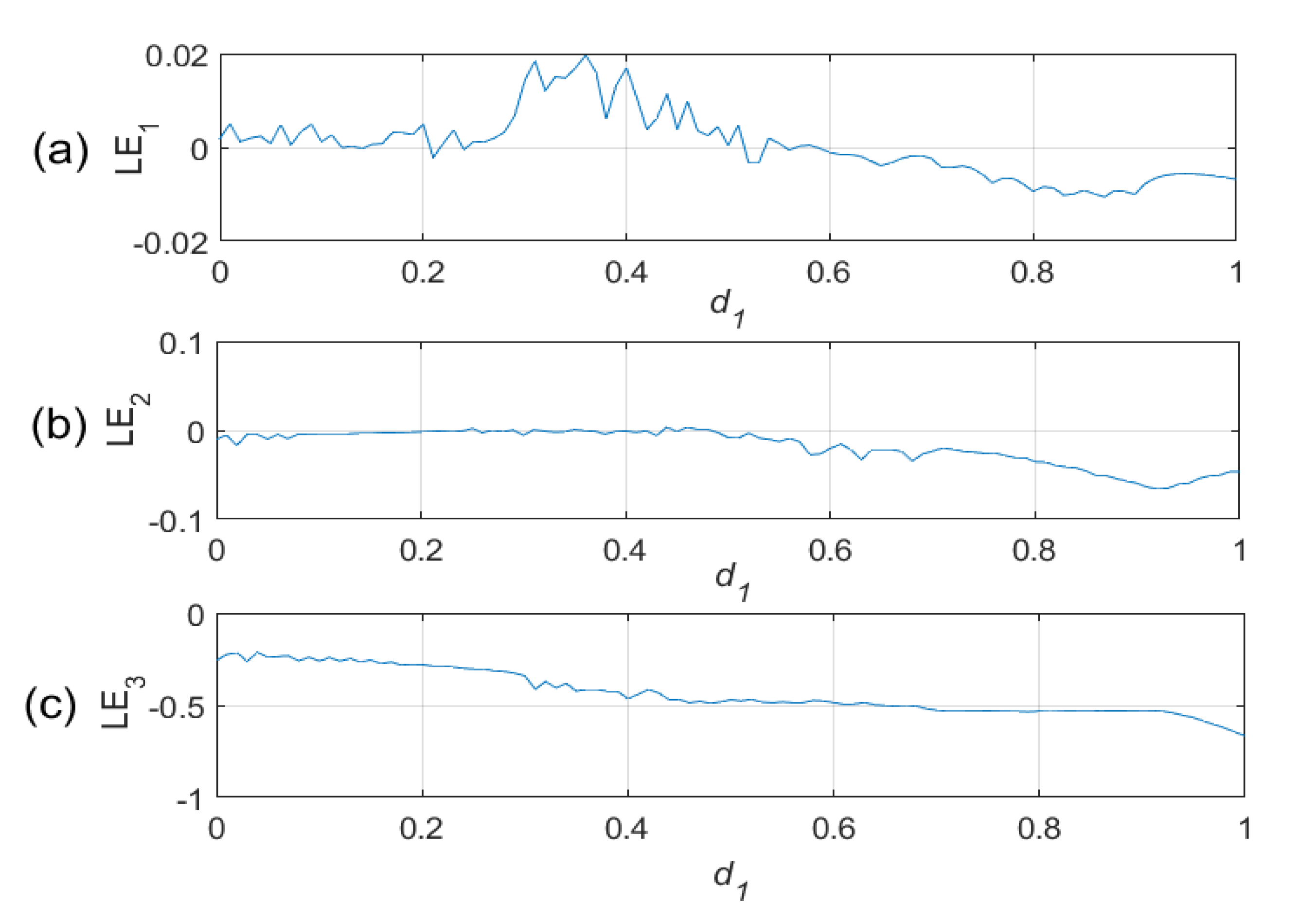
Since the impact of mortality of species $Y$ has a key effect on the ecosystem, the dynamics of system (4) with the varying parameter $d_1$ (positive correlation with mortality) is analyzed in this subsection. Letting parameter $d_1$ be varying from 0 to 1, and parameters $a_1,a_2,b_1,d_1,d_2$ be fixed as in Table 1, the Lyapunov exponents of system (4) are calculated, as shown in Figure 4. $L{E}_1$ is the largest Lyapunov exponent, as shown in Figure 4a, the others are less than zero, as shown in Figure 4b,c, respectively. It can be seen from Figure 4a that $L{E}_1$ is positive in the interval (0.24, 0.51), and negative in the interval (0.52, 1). These indicate that the three-species food-chain ecosystem has chaotic and periodic behaviors with the different parameters $d_1$, which predicts that the balance of the ecosystem can be realized by adjusting the parameter $d_1$.

When the parameters $d_1$, $D_1$ and $R_0$ satisfy (in Section 2)

$$d_1=\frac{D_1}{R_0}$$

(11)

and the intrinsic growth rate $R_0$ is a constant, the parameter $d_1$ is positively correlated with the natural death rate $D_1$ of the species $Y$. The parameter $d_1$ represents the natural death rate of species $Y$, and $d_1=0$ represents the species $Y$ does not die due to its own factors and $d_1=1$ represents the species $Y$ becomes extinct. It can be seen that the changes of the natural death rate of the species have a great effect on the dynamics of the three-species food-chain ecosystem.

4. The Dynamics of the Fractional-Order Ecosystem

4.1. A Necessary Condition for Generating Chaos

System (4) is next extended to fractional-order form, which is described by:

$$\{\begin{array}{l}{D}^{q_1}x(t)=x(t)(1-x(t))-\frac{5x(t)y(t)}{1+2.9x(t)},\\ D^{q_2}y(t)=\frac{5x(t)y(t)}{1+2.9x(t)}-\frac{0.1y(t)z(t)}{1+2.15y(t)}-0.4y(t),\\ D^{q_3}z(t)=\frac{0.1y(t)z(t)}{1+2.15y(t)}-0.01z(t),\\ x(0)=x_0>0,\\ y(0)=y_0>0,\\ z(0)=z_0>0.\end{array}$$

(12)

Based on the Caputo definition of the fractional derivative:

$${}_0^C{\mathrm{D}}_t^q\mathrm{f}\left(\mathrm{t}\right)=\frac{1}{\Gamma (n-q)}{\displaystyle {\int }_0^t\frac{f^{(n)}(s)}{{(t-s)}^{q+1-n}}}ds,$$

(13)

where $q>0$, $n-1<q<n$, $n\in N^{*}.$ Such $D^{q_i}=\frac{d^{q_i}}{d{t}^{q_i}}$, and $0<q_i<1\left(i=1,2,3\right)$. The dynamics of system (12) and the effect of the order of the fractional-order on the system will be are analyzed and explored in this section. Next, the equilibria and their stability of the system are discussed first.

Letting the right-hand side of the first three equations of system (12) be zero yields the six equilibria of the system as follows:$E_1=(0.8098,0.1274,10.3085),$$E_2=(0.1042,0.2333,0),$$E_3=(1,0,0),$ $E_4=(0,0,0),$$E_5=(0,0.1274,-5.0955),$$E_6=(-0.1546,0.1274,-22.9458)$.

The Jacobian matrix of the system is calculated at the equilibrium $(x^{\ast },y^{\ast },z^{\ast })$ as follows:

$$J=\left[\begin{array}{ccc}1-2x^{\ast }-\frac{5y^{\ast }}{{(1+2.9x^{\ast })}^2}& -\frac{5x^{\ast }}{1+2.9x^{\ast }}& 0\\ \frac{5y^{\ast }}{{(1+2.9x^{\ast })}^2}& \frac{5x^{\ast }}{1+2.9x^{\ast }}-\frac{0.1z^{\ast }}{{(1+2.15y^{\ast })}^2}-0.4& -\frac{0.1y^{\ast }}{1+2.15y^{\ast }}\\ 0& \frac{0.1z^{\ast }}{{(1+2.15y^{\ast })}^2}& \frac{0.1y^{\ast }}{1+2.15y^{\ast }}-0.01\end{array}\right].$$

The number of species is positive because zero means extinction. Only the equilibrium $E_1$ satisfies that all components are greater than zero, the stability of the system is to discuss here. The values of the equilibrium $E_1$ are substituted into J, the Jacobian matrix $J_1$ is

$$J_1=\left[\begin{array}{ccc}-0.6764& -1.2092& 0\\ 0.0568& 0.1740& -0.01\\ 0& 0.6352& 0\end{array}\right].$$

Its eigenvalues are ${\lambda }_1=-0.5875,$ ${\lambda }_{2,3}=0.0425\pm 0.0742i.$ The system has a negative real eigenvalue, and two conjugate complex eigenvalues with positive real parts, so $E_1$ is an unstable saddle-focus with index 2.

Based on the stability theory of fractional-order systems, a necessary condition for generating chaos is instability of the equilibria (See [41] for details). For the fractional-order ecosystem $D^{\alpha }F(X)=f(X)$, the parameter $\alpha$ satisfies:

$$\tan (\alpha \frac{\pi }{2})>\frac{\left|\mathrm{Im}(\lambda )\right|}{\mathrm{Re}(\lambda )}\Rightarrow \frac{\alpha \pi }{2}>\arctan (\frac{\left|\mathrm{Im}(\lambda )\right|}{\mathrm{Re}(\lambda )}),$$

(14)

where the order $\alpha =q_1=q_2=q_3$. According to the conjugate complex roots obtained above, one has:

$$\frac{\alpha \pi }{2}>\left|\arg \left({\lambda }_2\right)\right|=\left|\arg \left({\lambda }_3\right)\right|=\left|\arctan \left(\frac{0.0742}{0.0425}\right)\right|=\frac{0.6689\pi }{2}.$$

(15)

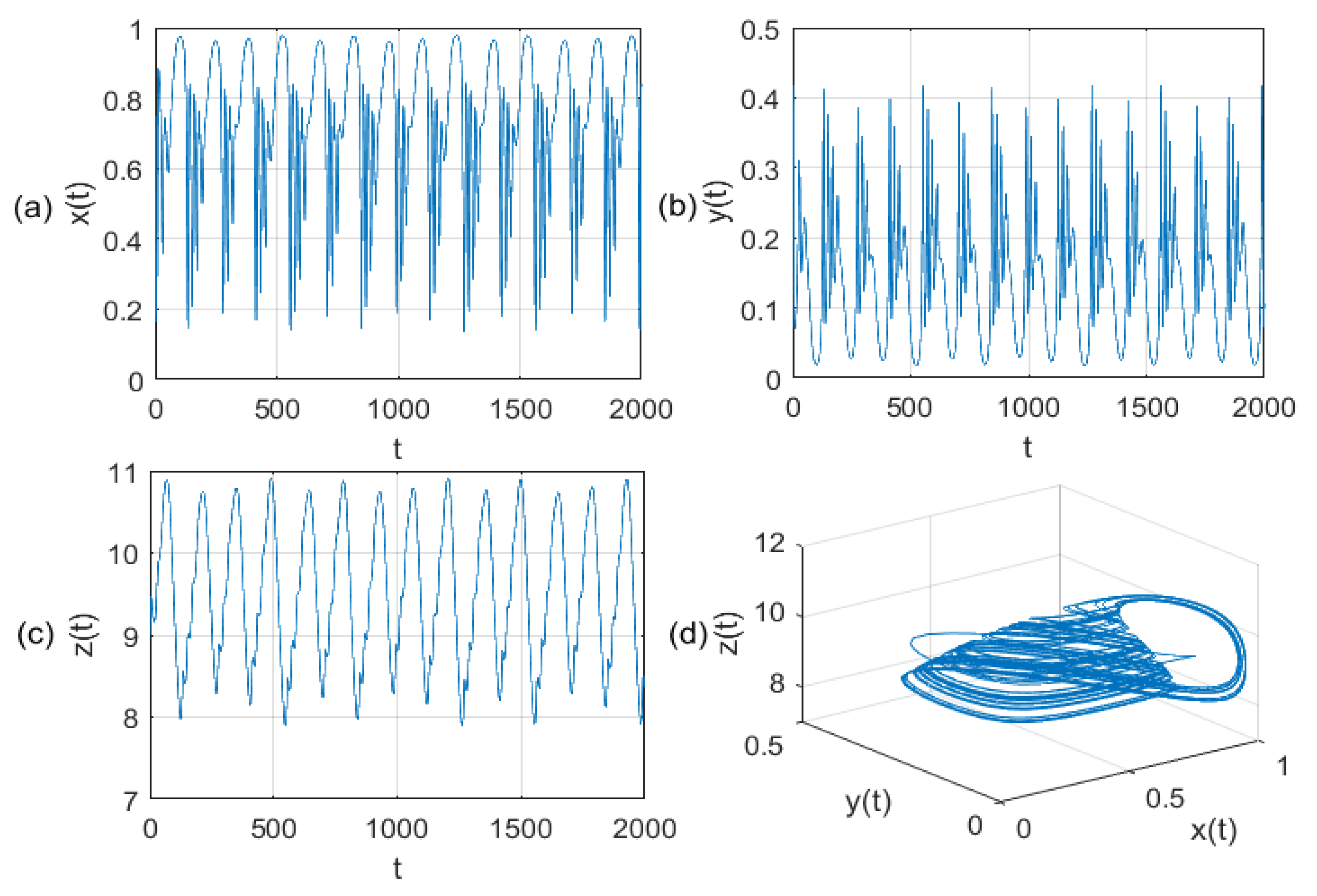
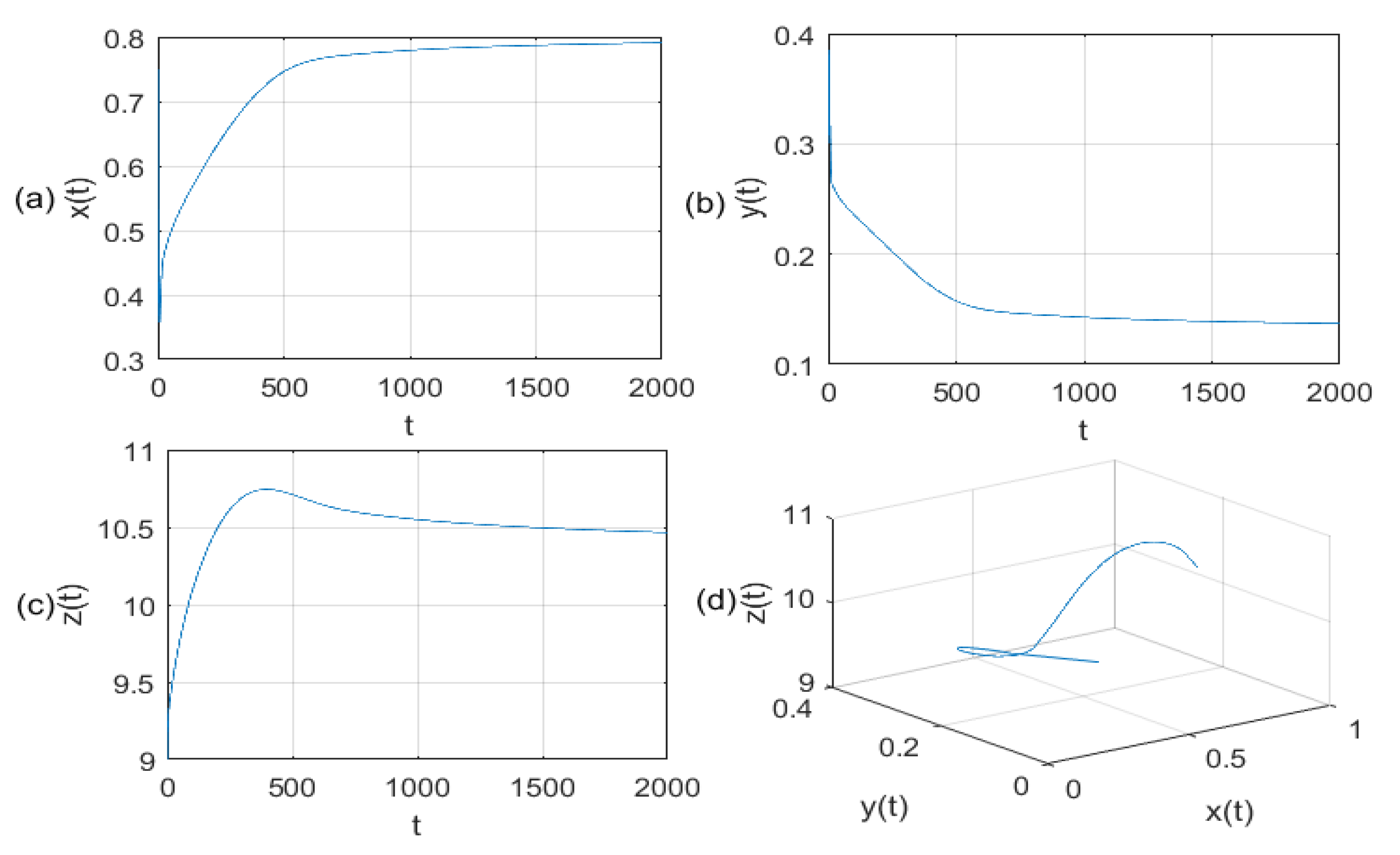
According the chaos theory [41], the necessary condition for chaos is the order $\alpha >0.6689$, which is the minimum order for generating chaos. Letting $\alpha =0.985$ yields a teacup chaotic attractor, as shown in Figure 5. The corresponding time-domain waves of the system are given in Figure 5a–c, respectively, and the orbit is shown in Figure 5d. This verifies the existence of chaos. When $\alpha <0.6689$, the system is non-chaotic, as shown in Figure 6, with the order $\alpha =0.6$. It can be seen from Figure 6a–c that the orbits of $x(t)$, $y(t)$ and $z(t)$ are asymptotically stable, and from Figure 6d the system tends to a fixed point. This indicates that the ecosystem of these three species can gradually reach a stable balance.

4.2. Dynamics of the Ecosystem with the Varying Parameter $b_1$

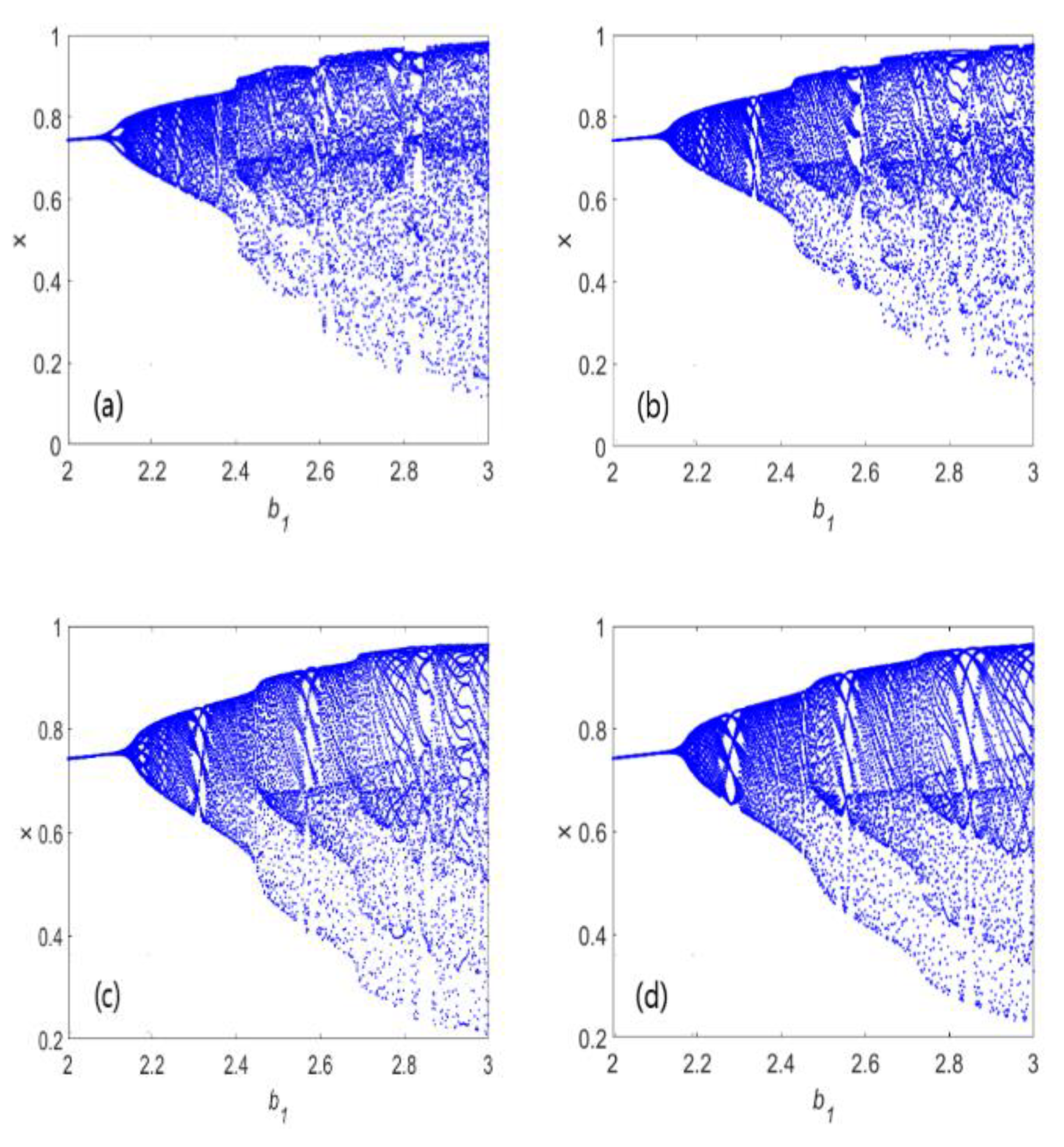
To analyze complex dynamics with different orders, the bifurcation diagrams are used in this subsection. Let the parameters $a_1,a_2,b_2,d_1,d_2$ be fixed as Table 1 and the parameter $b_1$ varies in the interval [2,3], the bifurcation diagrams with different orders are obtained, as shown in Figure 7.

Comparing the corresponding bifurcation diagrams of different orders shows that the order has different effects on the dynamic characterization of the ecosystem. In the specific range of order (0.95, 0.985), the first period-doubling bifurcation point defers with the decrease of order, which causes the value of corresponding parameter $b_1$ to increase. The values of the bifurcation point are inversely proportional to the values of the order, and the carrying capacity $K_0$ of the species $X$ increases with the decrease of the system order. Thus, the choice of order is a key to accurately describe the dynamics of the ecosystem.

4.3. Dynamics of the Ecosystem with the Varying Parameter $d_1$

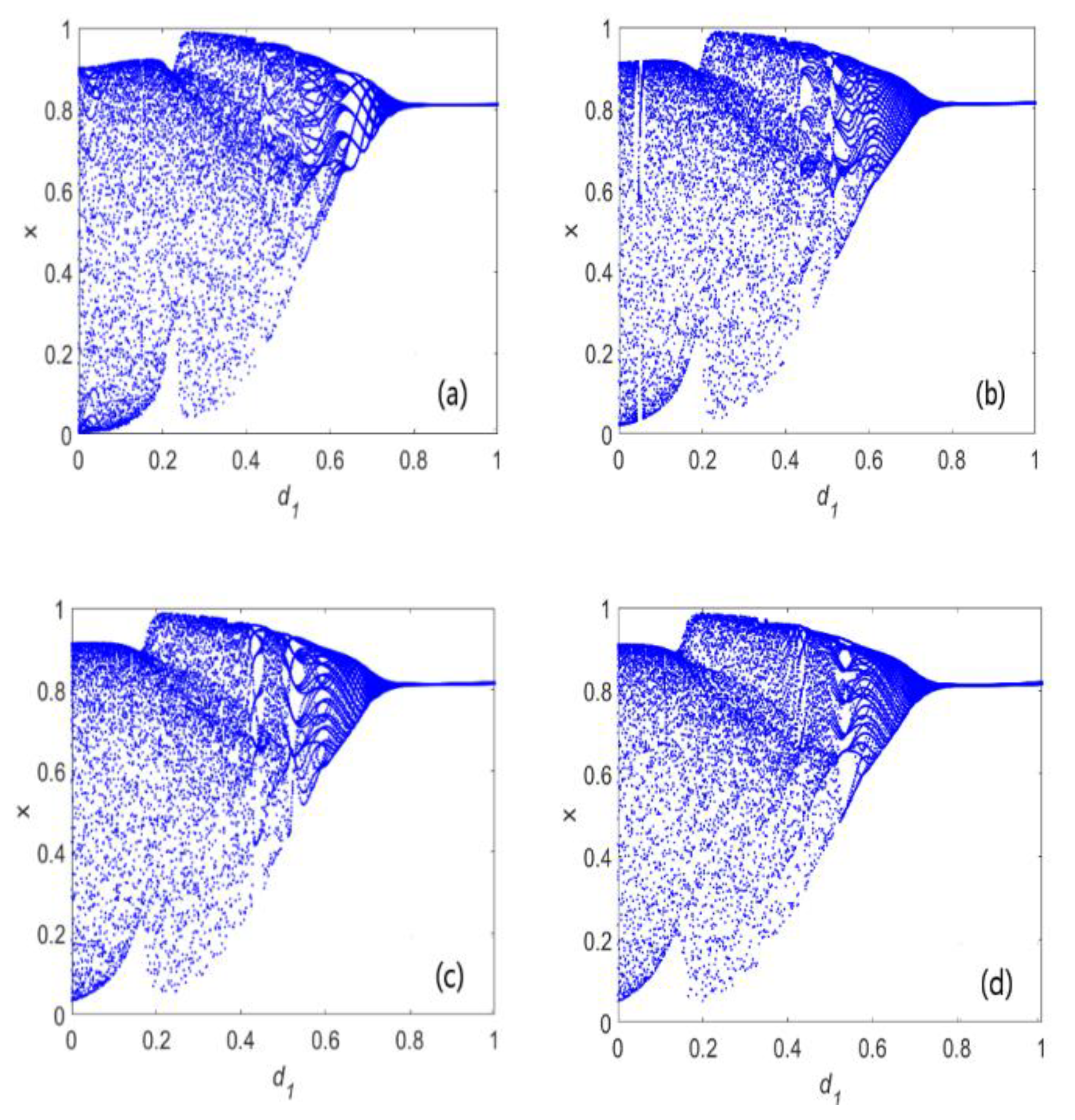
Next, $d_1$ is used as the control parameter to explore the dynamic behaviors of the system. Let parameters $a_1,a_2,b_1,b_2,d_2$ be fixed as Table 1, the bifurcation diagrams are obtained, as shown in Figure 8, with the parameter $d_1$ being in the interval (0, 1). It can be seen from Figure 8 that the system enter chaos by the reverse period-doubling bifurcation and the first bifurcation point decreases with the decrease of the order in the specific range (0.95, 0.985), which causes the value of the corresponding parameter $d_1$ to decrease.

The value of the bifurcation point is proportional to the value of the order, and the natural death rate of the species $Y$ decreases with the decrease of the system order. The choice of system order has effects on the natural death rate of the species $Y$.

It is concluded that the choice of order is a key to accurately describe the dynamics of the ecosystem, and has a significant effect on the dynamic of the fractional-order three-species food-chain system.

5. Chaos Control of the Fractional-Order Ecosystem

To eliminate the negative impacts of chaos on the dynamic balance of species number, the control of the three-species food chain is implemented to realize the stability of the system by feedback control method in this section. The Routh–Hurwitz criterion is an algebraic criterion that determines the stability of the system, which is adopted to determine the position of the eigenvalues in the S-plane. Then the stability margin of the controlled system is measured by the Routh–Hurwitz criterion.

The controlled system is first given by

$$\{\begin{array}{l}{D}^{q_1}x(t)=x(t)(1-x(t))-\frac{5x(t)y(t)}{1+2.9x(t)}-u_1,\\ D^{q_2}y(t)=\frac{5x(t)y(t)}{1+2.9x(t)}-\frac{0.1y(t)z(t)}{1+2.15y(t)}-0.4y(t)-u_2,\\ D^{q_3}z(t)=\frac{0.1y(t)z(t)}{1+2.15y(t)}-0.01z(t)-u_3,\\ x(0)=x_0>0,\\ y(0)=y_0>0,\\ z(0)=z_0>0,\end{array}$$

(16)

where $u_i\left(i=1,2,3\right)$ are the external control inputs, the control law has the following form:

$$\{\begin{array}{c}{u}_1=k_1\left(x(t)-x^{\ast }(t)\right),\\ u_2=k_2\left(y(t)-y^{\ast }(t)\right),\\ u_3=k_3\left(z(t)-z^{\ast }(t)\right),\end{array}$$

(17)

where $\left(x^{\ast }(t),y^{\ast }(t),z^{\ast }(t)\right)$ is the unstable equilibrium of system (4), and $k_i\left(i=1,2,3\right)$ are the feedback gains.

The controlled differential equations have the following form

$$\{\begin{array}{l}{D}^{q_1}x(t)=x(t)(1-x(t))-\frac{5x(t)y(t)}{1+2.9x(t)}-k_1\left(x\left(t\right)-0.8098\right),\\ D^{q_2}y(t)=\frac{5x(t)y(t)}{1+2.9x(t)}-\frac{0.1y(t)z(t)}{1+2.15y(t)}-0.4y(t)-k_2\left(y\left(t\right)-0.1274\right),\\ D^{q_3}z(t)=\frac{0.1y(t)z(t)}{1+2.15y(t)}-0.01z(t)-k_3\left(z\left(t\right)-10.3085\right),\\ x(0)=x_0>0,\\ y(0)=y_0>0,\\ z(0)=z_0>0.\end{array}$$

(18)

To apply the Routh–Hurwitz criterion, system (18) is linearized first. The Jacobian matrix of the system is

$$J_2=\left[\begin{array}{ccc}-2x-\frac{5y}{{\left(-1+2.9x\right)}^2}+\left(1-k_1\right)& -\frac{5x}{1+2.9x}& 0\\ \frac{5y}{{\left(1+2.9x\right)}^2}& \frac{5x}{1+2.9x}-\frac{0.1z}{{\left(1+2.15y\right)}^2}+\left(-0.4-k_2\right)& -\frac{0.1y}{1+2.15y}\\ 0& \frac{0.1z}{{\left(1+2.15y\right)}^2}& \frac{0.1y}{1+2.15y}+\left(-0.01-k_3\right)\end{array}\right].$$

The characteristic equation of the system is

$$\begin{array}{l}f\left(\lambda \right)={\lambda }^3+\left(k_1+k_2+k_3+\frac{314}{625}\right){\lambda }^2\\ +\left(k_1{k}_2+k_1{k}_3+k_2{k}_3+\frac{-87}{500}{k}_1+\frac{1691}{2500}{k}_2+\frac{314}{625}{k}_3+\frac{-266619}{6250000}\right)\lambda \\ +k_1{k}_2{k}_3+\frac{-87}{500}{k}_1{k}_3+\frac{1691}{2500}{k}_2{k}_3+\frac{397}{62500}{k}_1+\frac{-306319}{6250000}{k}_3+\frac{4953518943508485}{1152921504606846976}.\end{array}$$

(19)

The corresponding coefficients are

$$\{\begin{array}{l}{a}_3=1,\\ a_2=k_1+k_2+k_3+\frac{314}{625},\\ a_1=k_1{k}_2+k_1{k}_3+k_2{k}_3+\frac{-87}{500}{k}_1+\frac{1691}{2500}{k}_2+\frac{314}{625}{k}_3+\frac{-266619}{6250000},\\ a_0=k_1{k}_2{k}_3+\frac{-87}{500}{k}_1{k}_3+\frac{1691}{2500}{k}_2{k}_3+\frac{397}{62500}{k}_1+\frac{-306319}{6250000}{k}_3+\frac{4953518943508485}{1152921504606846976}.\end{array}$$

(20)

Letting the feedback gains $k_1=1,k_2=5,k_3=10$ of the system yields $a_3=1>0,$ $a_2=16.5024>0,$ $a_1=73.1893>0$, $a_0=81.6005>0$. Thus, ones have $f\left(\lambda \right)={\lambda }^3+16.5024{\lambda }^2+73.1893\lambda +81.6005$. All coefficients are positive real values, which meets the necessary conditions of stability of the system. The corresponding Routh array is obtained, as shown in

Table 2. The Routh array with $k_1=1,k_2=5,k_3=10$.

Terms	Coefficients
${\lambda }^3$	1	73.1893
${\lambda }^2$	16.5024	81.6005
${\lambda }^1$	68.2446	0
${\lambda }^0$	81.6005

.

The values of the first column of the Routh array are all positive, which confirms that the system is asymptotically stable based on the Routh–Hurwitz criterion. In fact, the roots of the characteristic equation are ${\lambda }_1=-9.9988$, ${\lambda }_2=-0.4053$, and ${\lambda }_3=-1.6984$, three roots are all negative real values. Further, the evolution of the controlled system (18) is obtained, as shown in Figure 9. It can be seen from Figure 9a–c that the orbits of states $x(t)$, $y(t)$ and $z(t)$ are asymptotically stable, and from Figure 9d the system tends to a stable point. These indicate that the system is asymptotically stable.

The values of feedback gains $k_1$, $k_2$ and $k_3$ are all positive, it indicates the three species of the system needs artificial fishing to adjust it. The numbers of fishing species $X$, $Y$ and $Z$ are 1, 5, and 10 times of the number of existing species exceeding their equilibrium, respectively. The chaos control of the system is realized by selecting specific feedback gains, which confirms that the feedback control method is effective. That being said, manual intervention, such as artificial deliberate protection or control, system can realize the chaos of the food chain to the stable state and achieve the long-term development of the ecosystem.

The detection of the stability margin of the controlled system is explored in the subsection. Substituting $\lambda =s-m$ into $f\left(\lambda \right)$ yields the characteristic equation as follows:

$$\begin{array}{ll}f\left(s\right)& ={\left(s-m\right)}^3+16.5024{\left(s-m\right)}^2+73.1893\left(s-m\right)+81.6005\\ & =s^3+\left(-3m+16.5024\right)s^2+\left(3m^2-33.0048m+73.1893\right)s\\ & +\left(-m^3+16.5024m^2-73.1893m+81.6005\right),\end{array}$$

(21)

where the stability margin $m_i(i=1,2,3,4)$ are positive. To explore the stability of the system, the Routh array of Equation (21) is given, as shown in

Table 3. The Routh array with $\lambda =s-m$.

Terms	Coefficients
$s^3$	1	3m2 − 33.0048m + 73.1893
$s^2$	−3m + 16.5024	−m3 + 16.5024m2 − 73.1893m + 81.6005
$s^1$	n	0
$s^0$	−m3 + 16.5024m2 − 73.1893m + 81.6005

.

In Table 3, the symbol $n$ is given below:

$$n=\frac{n_1{m}^3-n_2{m}^2+n_{3}m-n_4}{n_{5}m-n_6},$$

(22)

and

$$\begin{array}{c}{n}_1=219902325552\times {10}^8,n_2=362891613724213248\times {10}^4,\\ n_3=18995080734745441759488,n_4=30956711515873565050625,\\ n_5=824633720832\times {10}^8,n_6=4536145175526656\times {10}^4.\end{array}$$

(23)

When the coefficients of term $s$ and all values of the first column of the Routh array are positive, the system is stable. Therefore, the stability range of the system is calculated as $0<m<1.6984$, which indicates that the stability margin of the controlled system is 1.6984.

6. Conclusions

In this paper, a fractional-order three-species food-chain ecosystem is presented, which shows some unique dynamic behaviors. The chaotic state and the range of order with chaos of the system are confirmed. The bifurcation analysis with different orders verifies that the choice of order is extremely important for accurately characterizing the dynamics of the system. The result shows that the carrying capacity and mortality rate of each species have a great influence on the stability and development of the ecosystem under the certain conditions, which has the potential significance in practical applications. The stability of the fractional-order chaotic ecosystem is adjusted by the feedback control method, which generate a good effect. Moreover, the stability margin of the controlled fractional-order ecosystem is obtained by theory analysis and numerical simulations.

These subjects about the discretization of the fractional-order system, control methods of fractional-order system, and the dynamic analysis of corresponding time delay fractional system and others deserve further study in the near future.

References

- Grigorenko, I.; Grigorenko, E. Chaotic dynamics of the fractional Lorenz system. Phys. Rev. Lett. 2003, 91, 034101. [Google Scholar] [CrossRef]
- Chen, G.; Ueta, T. Yet another chaotic attractor. Int. J. Bifurc. Chaos 1999, 9, 1465–1466. [Google Scholar] [CrossRef]
- Zhou, P.; Ding, R.; Cao, Y. Multi drive-one response synchronization for fractional-order chaotic systems. Nonlinear Dyn. 2012, 70, 1263–1271. [Google Scholar] [CrossRef]
- Mihailović, D.T.; Mimić, G.; Arsenić, I. Climate predictions: The chaos and complexity in climate models. Adv. Meteorol. 2014, 2014, 1–14. [Google Scholar] [CrossRef]
- Chang, H.; Li, Y.; Yuan, F.; Chen, G. Extreme multistability with hidden attractors in a simplest memristor-based circuit. Int. J. Bifur. Chaos 2019, 29, 1950086. [Google Scholar] [CrossRef]
- Yuan, F.; Li, Y. A chaotic circuit constructed by a memristor, a memcapacitor and a meminductor. Chaos 2019, 29, 101101. [Google Scholar] [CrossRef] [PubMed]
- Rossler, O.E.; Rossler, R. Chaos in physiology. Integr. Physiol. Behav. Sci. 1994, 29, 328–333. [Google Scholar] [CrossRef] [PubMed]
- Bob, P. Chaos, cognition and disordered brain. Act. Nerv. Super. 2008, 50, 114–117. [Google Scholar] [CrossRef] [Green Version]
- Ahmed, E. Fractals and chaos in cancer models. Int. J. Theor. Phys. 1993, 32, 353–355. [Google Scholar] [CrossRef]
- Adrangi, B.; Allender, M.; Chatrath, A.; Raffiee, K. Nonlinearities and chaos: Evidence from exchange rates. Atl. Econ. J. 2010, 38, 247–248. [Google Scholar] [CrossRef]
- Park, J. Biodiversity in the cyclic competition system of three species according to the emergence of mutant species. Chaos 2018, 28, 053111. [Google Scholar] [CrossRef] [PubMed]
- Hastings, A.; Powell, T. Chaos in a three-species food chain. Ecology 1991, 72, 896–903. [Google Scholar] [CrossRef]
- Baek, H.; Lim, Y.; Lim, D. A three-species food chain system with two types of functional responses. Abstr. Appl. Anal. 2011, 2011, 155–159. [Google Scholar]
- Chakraborty, K.; Das, K.; Yu, H.G. Modeling and analysis of a modified Leslie-Gower type three species food chain model with an impulsive control strategy. Nonlinear Anal. Hybrid Syst. 2015, 15, 171–184. [Google Scholar] [CrossRef]
- Nath, B.; Kumari, N.; Kumar, V.; Das, K.P. Refugia and Allee effect in prey species stabilize chaos in a tri-trophic food chain model. Differ. Equ. Dyn. Syst. 2019, 1–27. [Google Scholar] [CrossRef]
- Samanta, S.; Chowdhury, T.; Chattopadhyay, J. Mathematical modeling of cascading migration in a tri-trophic food-chain system. J. Biol. Phys. 2013, 39, 469–487. [Google Scholar] [CrossRef] [Green Version]
- Das, K.P.; Roy, P.; Ghosh, S.; Maiti, S. External source of infection and nutritional efficiency control chaos in a predator-prey model with disease in the predator. Biophys. Rev. Lett. 2017, 12, 87–115. [Google Scholar]
- Panday, P.; Pal, N.; Samanta, S.; Chattopadhyay, J. Stability and bifurcation analysis of a three-species food chain model with fear. Int. J. Bifurc. Chaos 2018, 28, 1850009. [Google Scholar] [CrossRef]
- Sadhu, S.; Kuehn, C. Stochastic mixed-mode oscillations in a three-species predator-prey model. Chaos 2018, 28, 033606. [Google Scholar] [CrossRef]
- Meng, X.; Qin, N. Bifurcation analysis of a food chain system incorporating time delay and the disease spreading among prey species. In Proceedings of the Chinese Control and Decision Conference (CCDC), Shenyang, China, 9–11 June 2018; pp. 68–73. [Google Scholar]
- Hsu, T.H. Number and stability of relaxation oscillations for predator-prey systems with small death rates. SIAM J. Appl. Dyn. Syst. 2019, 18, 33–67. [Google Scholar] [CrossRef]
- Ishaque, W.; Din, Q.; Taj, M.; Iqbal, M.A. Bifurcation and chaos control in a discrete-time predator-prey model with nonlinear saturated incidence rate and parasite interaction. Adv. Differ. Equ. 2019, 2019, 1–16. [Google Scholar] [CrossRef] [Green Version]
- Hanert, E.; Schumacher, E.; Deleersnijder, E. Front dynamics in fractional-order epidemic models. J. Theor. Biol. 2011, 279, 9–16. [Google Scholar] [CrossRef] [PubMed] [Green Version]
- Hanert, E. Front dynamics in a two-species competition model driven by Lévy flights. J. Theor. Biol. 2012, 300, 134–142. [Google Scholar] [CrossRef] [PubMed]
- Ji, G.; Ge, Q.; Xu, J. Dynamic behaviors of a fractional order two-species cooperative systems with harvesting. Chaos Solitons Fractals 2016, 92, 51–55. [Google Scholar] [CrossRef]
- Matouk, A.E.; Elsadany, A.A.; Ahmed, E.; Agiza, H.N. Dynamical behavior of fractional-order Hastings-Powell food chain model and its discretization. Commun. Nonlinear Sci. Numer. Simul. 2015, 27, 153–167. [Google Scholar] [CrossRef]
- Gao, Y.; Zhao, W. Stability analysis for the fractional-order single-species model with the dispersal. In Proceedings of the 29th Chinese Control and Decision Conference (CCDC), Chongqing, China, 28–30 May 2017; pp. 7822–7826. [Google Scholar]
- Zhou, X.; Wu, Z.; Wang, Z.; Zhou, T. Stability and Hopf bifurcation analysis in a fractional-order delayed paddy ecosystem. Adv. Differ. Equ. 2018, 2018, 1–14. [Google Scholar] [CrossRef]
- Chinnathambi, R.; Rihan, F.A. Stability of fractional-order prey-predator system with time-delay and monod-haldane functional response. Nonlinear Dyn. 2018, 92, 1–12. [Google Scholar] [CrossRef]
- Li, W.; Huang, L.; Ji, J. Periodic solution and its stability of a delayed Beddington-DeAngelis type predator-prey system with discontinuous control strategy. Math. Methods Appl. Sci. 2019, 42, 4498–4515. [Google Scholar] [CrossRef]
- Alidousti, J.; Ghahfarokhi, M.M. Dynamical behavior of a fractional three-species food chain model. Nonlinear Dyn. 2018, 95, 1841–1858. [Google Scholar] [CrossRef]
- Zheng, K.; Zhou, X.; Wu, Z.; Wang, Z.; Zhou, T. Hopf bifurcation controlling for a fractional order delayed paddy ecosystem in the fallow season. Adv. Differ. Equ. 2019, 201, 307. [Google Scholar] [CrossRef] [Green Version]
- Wu, X.J.; Li, J.; Upadhyay, R.K. Chaos control and synchronization of a three-species food chain model via Holling functional response. Int. J. Comput. Math. 2010, 87, 199–214. [Google Scholar] [CrossRef]
- Din, Q. Complexity and chaos control in a discrete-time prey-predator model. Commun. Nonlinear Sci. Numer. Simul. 2017, 49, 113–134. [Google Scholar] [CrossRef]
- Zhao, H.; Lin, Y.; Dai, Y. Bifurcation analysis and control of chaos for a hybrid ratio-dependent three species food chain. Appl. Math. Comput. 2011, 218, 1533–1546. [Google Scholar] [CrossRef]
- Chattopadhyay, J.; Pal, N.; Samanta, S.; Venturino, E.; Khan, Q.J.A. Chaos control via feeding switching in an omnivory system. Biosystems 2015, 138, 18–24. [Google Scholar] [CrossRef] [PubMed]
- Danca, M.F.; Chattopadhyay, J. Chaos control of Hastings-Powell model by combining chaotic motions. Chaos 2016, 26, 043106. [Google Scholar] [CrossRef] [PubMed] [Green Version]
- Singh, A.; Gakkhar, S. Controlling chaos in a food chain model. Math. Comput. Simul. 2015, 46, 913–915. [Google Scholar] [CrossRef]
- Parshad, R.D.; Quansah, E.; Black, K.; Beauregard, M. Biological control via “ecological” damping: An approach that attenuates non-target effects. Math. Biosci. 2016, 273, 23–44. [Google Scholar] [CrossRef] [Green Version]
- Marin, M.; Ellahi, R.; Chirilă, A. On solutions of Saint-Venant’s problems for elastic dipolar bodies with voids. Carpathian J. Math. 2017, 33, 219–232. [Google Scholar]
- Tavazoei, M.S.; Haeri, M. Chaotic attractors in incommensurate fractional order systems. Phys. D 2008, 237, 2628–2637. [Google Scholar] [CrossRef]
Figure 1.
The chaotic attractor of system (4). (a) x(t)-y(t); (b) x(t)-z(t); (c) y(t)-z(t); (d) x(t)-y(t)-z(t).
Figure 2.
Time-domain waves of system (4). (a) x(t)-t; (b) y(t)-t; (c) z(t)-t.
Figure 3.
The bifurcation diagram with the varying parameter .
Figure 4.
The Lyapunov exponents with the varying parameter . (a) ; (b) ; (c) .
Figure 5.
The teacup chaotic attractor and the time-domain waves of system (12) with . (a) x(t)-t; (b) y(t)-t; (c) z(t)-t; (d) x(t)-y(t)-z(t).
Figure 6.
Evolution of the system states with . (a) x(t)-t; (b) y(t)-t; (c) z(t)-t; (d) x(t)-y(t)-z(t).
Figure 7.
Bifurcation diagrams with the varying parameter (a) ; (b) ; (c) ; (d) .
Figure 8.
Bifurcation diagrams with the varying parameter . (a) , (b) , (c) , (d) .
Figure 9.
Evolution of the controlled system (18) with . (a) x(t)-t; (b) y(t)-t; (c) z(t)-t; (d) x(t)-y(t)-z(t).