Stochastic Brennan–Schwartz Diffusion Process: Statistical Computation and Application

Abstract

In this paper, we study the one-dimensional homogeneous stochastic Brennan–Schwartz diffusion process. This model is a generalization of the homogeneous lognormal diffusion process. What is more, it is used in various contexts of financial mathematics, for example in deriving a numerical model for convertible bond prices. In this work, we obtain the probabilistic characteristics of the process such as the analytical expression, the trend functions (conditional and non-conditional), and the stationary distribution of the model. We also establish a methodology for the estimation of the parameters in the process: First, we estimate the drift parameters by the maximum likelihood approach, with continuous sampling. Then, we estimate the diffusion coefficient by a numerical approximation. Finally, to evaluate the capability of this process for modeling real data, we applied the stochastic Brennan–Schwartz diffusion process to study the evolution of electricity net consumption in Morocco.

1. Introduction

Stochastic diffusion models, such as continuous-time Markovian processes, are used to describe the evolution of phenomena in diverse fields. They have extensive domains of application in many areas of science, including biology, mathematical finance, growth phenomena, and energy consumption, especially electricity. For example, in mathematical finance, Vasicek presented a global form of the term structure of interest rates [1]; Brennan and Schwartz established an arbitration model concerning the term structure of interest rates [2]; thus, Albano and Giorno advised a stochastic diffusion process suitable for modeling the interest rate progress regarding time [3]. Furthermore, Nafidi et al. applied the square of the Brennan–Schwartz model to population growth; see [4]. Indeed, in growth phenomena, various authors have introduced stochastic versions of classical deterministic growth models especially in animal or cell populations, birth-death, energy, survival populations, life-testing experiments, and environmental studies. See, for example: Saha and Chakrabarti [5], Nafidi et al. [6], Di Crescenzo and Paraggio [7], Gutiérrez et al. [8], and Skiadas and Giovanis [9]. Diffusion processes are also examined in the field of electricity; in fact, many studies have been focused on the consumption of electrical energy; diverse works suggested a means of using stochastic diffusion processes to model the total consumption of electrical power and to forecast the consumption of electrical energy in relation to particular economic or climatologic variables, using statistical techniques. In this respect, see the works of Gutiérrez et al., who proposed a means of using stochastic diffusion processes to model the total consumption of electrical power in Morocco [10], and Nafidi et al., who modeled electric power consumption throughout a period of economic crisis [11].

In most cases, the methodology used in statistical inference is obtained from the likelihood function, which is a product of transition densities, and these are only known in special cases. Therefore, various authors studied and developed several methods to deal with this problem: Bibby and Sorensen [12], Kloeden and Platen [13], and Singer [14], without overlooking the wide-ranging review of the results given by Prakasa-Rao [15], who procured an extended list of references with respect to the subject.

The process examined in this paper is the stochastic Brennan–Schwartz Diffusion Process (BSDP), which is in financial mathematics used for example, by [16] in developing a model of discount bond option prices. In this work, we study the capability of applying the stochastic BSDP in another field, to describe the evolution of the electricity net consumption in Morocco and to predict future trends, by using the statistical inference in fitting and forecasting, from observed data.

In this study, we obtain the probabilistic characteristics of the stochastic BSDP like the solution, the trend functions, and the stationary distribution of the process, after which the drift coefficient is estimated by applying the likelihood approach, with continuous sampling. Then, the diffusion coefficient is estimated by a numerical approximation. Finally, in order to evaluate the capability of this process for modeling real data in the field of electricity, we apply the stochastic BSDP to study the evolution of electricity net consumption in Morocco.

2. The Model and Its Basic Probabilistic Characteristics

2.1. The Proposed Model

Let $\left\{x\left(t\right);t\in [t_0,T];t_0\ge 0\right\}$ be the one-dimensional homogeneous diffusion process, which is defined as the unique solution to the following Stochastic Differential Equation (SDE) (see [17]):

$$dx\left(t\right)=\left(\alpha x\left(t\right)+\beta \right)dt+\sigma x\left(t\right)dw\left(t\right),x\left(t_0\right)=x_{t_0},$$

(1)

where $\sigma >0$, $\alpha$, and $\beta$ are real parameters, $w\left(t\right)$ is a one-dimensional standard Wiener process, and $x_{t_0}>0$ is a fixed real value.

Note that when $\beta =0$, the homogeneous lognormal diffusion process is acquired as a specific case. This process has been studied in depth by [18,19].

2.2. The Analytical Expression of the Process

The analytical expression of the process can be obtained by referring to [13]. Remember that if:

$$dy\left(t\right)=\left(a_{1}y\left(t\right)+a_2\right)dt+\left(b_{1}y\left(t\right)+b_2\right)dw\left(t\right),y\left(t_0\right)=y_{t_0},$$

thus the solution of the previous equation has the following form:

$$y\left(t\right)=\mathsf{\Phi }\left(t\right)\left\{y_{t_0}+(a_2-b_1{b}_2){\int }_{t_0}^t\mathsf{\Phi }{\left(\tau \right)}^{-1}d\tau +b_2{\int }_{t_0}^t\mathsf{\Phi }{\left(\tau \right)}^{-1}dw\left(\tau \right)\right\},$$

where:

$$\mathsf{\Phi }\left(t\right)=\exp \left\{a_1(t-t_0)-\frac{1}{2}{b}_1^2(t-t_0)+b_1(w\left(t\right)-w\left(t_0\right))\right\}.$$

Therefore, in our case, by applying the previous result, the SDE Equation (1) has a unique solution $x\left(t\right)$, which is known in the field of stochastic finance (see for example [13]). Consequently, this solution has the following expression:

$$\begin{array}{ccc}\hfill x\left(t\right)& =& \left(x_{t_0}+\beta {\int }_{t_0}^t\exp \left[-\left(\alpha -\frac{{\sigma }^2}{2}\right)\left(\tau -t_0\right)-\sigma \left(w\left(\tau \right)-w\left(t_0\right)\right)\right]d\tau \right)\hfill \\ & & \left(\exp \left[\left(\alpha -\frac{{\sigma }^2}{2}\right)\left(t-t_0\right)+\sigma \left(w\left(t\right)-w\left(t_0\right)\right)\right]\right).\hfill \end{array}$$

2.3. The Trend Functions of the Process

Since the probability transition density function (ptdf) of the model is not known, we will use the following method described in [13] for obtaining the conditional and non-conditional trend functions of the process. The SDE in Equation (1) can be written in integral form as:

$$x\left(t\right)=x\left(s\right)+{\int }_s^t\left(\alpha x\left(\theta \right)+\beta \right)d\theta +\sigma {\int }_s^{t}x\left(\theta \right)dw\left(\theta \right),$$

from which we obtain:

$$\mathbb{E}\left(x\left(t\right)\mid x\left(s\right)=x_s\right)=x_s+\beta (t-s)+\alpha {\int }_s^t\mathbb{E}\left(x\left(\theta \right)\mid x\left(s\right)=x_s\right)d\theta .$$

Denoting this by $g\left(t\right)=\mathbb{E}\left(x\left(t\right)\mid x\left(s\right)=x_s\right)$, we then have:

$$g\left(t\right)=x_s+\beta (t-s)+\alpha {\int }_s^{t}g\left(\theta \right)d\theta ,$$

and deriving with respect to t, we conclude that the conditional trend function of the BSDP solves the following Ordinary Differential Equation (ODE):

$$g^{{}^{\prime }}\left(t\right)=\alpha g\left(t\right)+\beta ,g\left(s\right)=x_s,$$

the solution of the latter ODE without a second member has the following form:

$$g\left(t\right)=k\left(t\right)e^{\alpha t},$$

and by using the variation of the constant, we can deduce that:

$$k\left(t\right)=\frac{-\beta }{\alpha }{e}^{-\alpha t}+cte.$$

To determine the constant denoted as $cte$ in the previous equation, we use the initial condition $g\left(s\right)=x_s$, then we conclude that the unique solution of our ODE is given by:

$$g\left(t\right)=x_s{e}^{\alpha (t-s)}+\frac{\beta }{\alpha }\left(e^{\alpha (t-s)}-1\right).$$

Eventually, the conditional trend function of the model is given by:

$$\mathbb{E}(x\left(t\right)\mid x\left(s\right)=x_s)=x_s{e}^{\alpha (t-s)}+\frac{\beta }{\alpha }\left(e^{\alpha (t-s)}-1\right),$$

(2)

and by assuming the initial condition $\mathrm{P}\left(x\left(t_0\right)=x_{t_0}\right)=1$, the trend function of the process is:

$$\mathbb{E}\left(x\left(t\right)\right)=x_{t_0}{e}^{\alpha (t-t_0)}+\frac{\beta }{\alpha }\left(e^{\alpha (t-t_0)}-1\right).$$

(3)

2.4. Ergodicity and Stationary Distribution

We shall now determine the stationary distribution of the process, the density function, and the asymptotic moments.

In general (see [20,21]), a stochastic diffusion process $\left\{x\left(t\right),t\ge 0\right\}$, with state space $I=(l,r)$, is led by the ensuing SDE:

$$\begin{array}{c}\hfill dx\left(t\right)=a\left(x\left(t\right)\right)dt+b\left(x\left(t\right)\right)dw\left(t\right),x_0=x,\end{array}$$

where $w\left(t\right)$ is a standard Wiener process and the constant value x is independent of $w\left(t\right)$. We suppose that $a\left(x\right)$ and $b\left(x\right)$ are continuously differentiable.

Let ${\displaystyle s\left(z\right)=\exp \left\{-{\int }_{z_0}^z\frac{2a\left(u\right)}{b^2\left(u\right)}du\right\}}$ be the scale density function ($z_0$ is an arbitrary point inside I).

The speed density function is given by ${\displaystyle m\left(u\right)={\left(b^2\left(u\right)s\left(u\right)\right)}^{-1}.}$ We denote by:

$$S[x,y]={\int }_x^{y}s\left(u\right)du,S(l,y]=\underset{x\to l}{\lim }{\int }_x^{y}s\left(u\right)du\mathrm{and}S[x,r)=\underset{y\to r}{\lim }{\int }_x^{y}s\left(u\right)du,$$

where $l<x<y<r$. Then, if:

$$\begin{array}{c}\hfill S(l,y]=S[x,r)=\infty \mathrm{and}{\int }_l^{r}m\left(u\right)du<\infty ,\end{array}$$

the process $\left\{x\left(t\right),t\ge 0\right\}$ is ergodic, and its stationary density function is found to be:

$$f\left(x\right)=m\left(x\right)/{\int }_l^{r}m\left(u\right)du.$$

In our case, the drift and diffusion coefficient have the following form:

$$a\left(x\right)=\alpha x+\beta \mathrm{and}{b}^2\left(x\right)={\sigma }^2{x}^2,$$

and $I=(0,\infty )$. It follows that:

$$s\left(z\right)=k{z}^{-\frac{2\alpha }{{\sigma }^2}}{e}^{\frac{2\beta }{{\sigma }^{2}z}},\mathrm{with}k=z_0^{\frac{2\alpha }{{\sigma }^2}}{e}^{-\frac{2\beta }{{\sigma }^2{z}_0}},$$

and we have, for $0<x<y<\infty$:

$$\begin{array}{c}\hfill S[x,y]={\int }_x^{y}s\left(u\right)du=k{\int }_x^y{u}^{-\frac{2\alpha }{{\sigma }^2}}{e}^{\frac{2\beta }{{\sigma }^{2}u}}du.\end{array}$$

With the variable change $v=u^{-1}$, the previous expression is given by:

$$\begin{array}{c}\hfill S[x,y]=2k{\int }_{1/y}^{1/x}{v}^{\frac{2\alpha }{{\sigma }^2}-2}{e}^{\frac{-2\beta }{{\sigma }^2}v}dv.\end{array}$$

(4)

Then, taking the limit as x tends to zero in Equation (4), we conclude that, for $\beta >0$, $S(0,y]=\infty .$

Taking the limit when y tends to ∞ in Equation (4), we have, for ${\displaystyle \alpha \le \frac{{\sigma }^2}{2}}$, $S[x,\infty )=\infty$.

Consequently, we have for ${\displaystyle \alpha \le \frac{{\sigma }^2}{2}}$ and $\beta >0$,

$$S[x,\infty )=S(0,y]=\infty .$$

The speed density is given by:

$${\displaystyle m\left(x\right)=\frac{1}{k{\sigma }^2}{x}^{\frac{2\alpha }{{\sigma }^2}-2}{e}^{\frac{-2\beta }{{\sigma }^{2}x}},}$$

then we obtain:

$$\begin{array}{ccc}\hfill {\int }_0^{\infty }m\left(x\right)dx& =& \frac{1}{k{\sigma }^2}{\int }_0^{\infty }{x}^{\frac{2\alpha }{{\sigma }^2}-2}{e}^{\frac{-2\beta }{{\sigma }^{2}x}}dx\hfill \\ & =& \frac{1}{k{\sigma }^2}{\int }_0^{\infty }{v}^{\frac{-2\alpha }{{\sigma }^2}}{e}^{-\frac{2\beta }{{\sigma }^2}v}dv,\hfill \end{array}$$

and according to Gradstien et al. [22], for $\nu >0$ and $\mu >0$,

$${\int }_0^{\infty }{x}^{\nu -1}{e}^{-\mu x}dx={\mu }^{-\nu }\mathsf{\Gamma }\left(\nu \right);$$

for ${\displaystyle \alpha <\frac{{\sigma }^2}{2}}$ and $\beta >0$, we have:

$$\begin{array}{c}\hfill {\displaystyle {\int }_0^{\infty }m\left(x\right)dx=\frac{1}{k{\sigma }^2}{\left(\frac{2\beta }{{\sigma }^2}\right)}^{\left(\frac{2\alpha }{{\sigma }^2}-1\right)}\mathsf{\Gamma }\left(1-\frac{2\alpha }{{\sigma }^2}\right)<\infty .}\end{array}$$

Thus, by joining the two previous conditions, we conclude that for ${\displaystyle \alpha <\frac{{\sigma }^2}{2}}$ and $\beta >0$, the process is ergodic. Finally, for $\alpha <\frac{{\sigma }^2}{2}$ and $\beta >0$, the density function of the stationary distribution of the proposed model exists and is given by:

$$\begin{array}{c}\hfill {\displaystyle f\left(x\right)=\frac{{\left(\frac{2\beta }{{\sigma }^2}\right)}^{1-\frac{2\alpha }{{\sigma }^2}}{x}^{\frac{2\alpha }{{\sigma }^2}-2}\exp (-\frac{2\beta }{{\sigma }^{2}x})}{\mathsf{\Gamma }\left(1-\frac{2\alpha }{{\sigma }^2}\right)}.}\end{array}$$

(5)

where $\mathsf{\Gamma }(.)$ is the Gamma function. It can be easily demonstrated that the function f is the density of the inverse of the Gamma distribution with the parameters ${\displaystyle 1-\frac{2\alpha }{{\sigma }^2}}$ and ${\displaystyle \frac{{\sigma }^2}{2\beta }}$.

The expression (5) can be used to calculate the asymptotic moment of order k, then we have for ${\displaystyle 1-\frac{2\alpha }{{\sigma }^2}>k}$ and $\beta >0$:

$$\begin{array}{c}\hfill \mathbb{E}\left[X_{\infty }^k\right]={\int }_0^{\infty }{x}^{k}f\left(x\right)dx={\left(\frac{2\beta }{{\sigma }^2}\right)}^k\frac{\mathsf{\Gamma }(1-\frac{2\alpha }{{\sigma }^2}-k)}{\mathsf{\Gamma }(1-\frac{2\alpha }{{\sigma }^2})}.\end{array}$$

The asymptotic trend function of the process is obtained by using the properties of the Euler function, ($k=1$), for $\beta >0$ and $\alpha <0$:

$$\mathbb{E}\left[X_{\infty }\right]=-\frac{\beta }{\alpha }.$$

By taking the limit when t tends to ∞ in Equation (3), we get for $\beta >0$ and $\alpha <0$:

$$\begin{array}{c}\hfill \underset{t\to \infty }{\lim }\mathbb{E}\left(x\left(t\right)\right)=\mathbb{E}\left(X_{\infty }\right).\end{array}$$

This implies that the limit of the trend function in Equation (3) (when t tends to ∞) corresponds to the asymptotic trend function.

3. Statistical Inference in the Model

We will now estimate the parameters of the proposed model. The drift parameters ($\alpha$ and $\beta$) are estimated by the maximum likelihood method, with continuous sampling. Then, for the parameter of the diffusion coefficient, we shall apply the approximation method considered by Chesney and Elliot [23].

3.1. Likelihood Estimation of Drift Parameters

Consider the one-dimensional diffusion process defined by the following vectorial form:

$$dx\left(t\right)=A_t\left(x\left(t\right)\right)\theta +B_t\left(x\left(t\right)\right)dw\left(t\right),t_0\le t\le T,$$

where $\theta \in {\mathbb{R}}^k$, $A_t$ is a k-dimensional vector, and $B_t$ is $\mathbb{R}$-valued depending only on the sample path up to a given instant. Suppose that the latter equation has a unique solution for every $\theta$. The maximum likelihood estimator of the vector $\theta$ is (see [9,24,25,26,27]):

$$\begin{array}{c}\hfill \widehat{\theta }=S_T^{-1}{H}_T,\end{array}$$

where $H_T$ is the following k-dimensional vector:

$$\begin{array}{c}\hfill H_T={\int }_{t_0}^T{A}_t^{\ast }\left(x\left(t\right)\right){\left(B_t\left(x\left(t\right)\right)B_t\left(x\left(t\right)\right)\right)}^{-1}dx\left(t\right),\end{array}$$

$S_T$ is the k × k matrix:

$$\begin{array}{c}\hfill S_T={\int }_{t_0}^T{A}_t^{\ast }\left(x\left(t\right)\right){\left(B_t\left(x\left(t\right)\right)B_t\left(x\left(t\right)\right)\right)}^{-1}{A}_t\left(x\left(t\right)\right)dt,\end{array}$$

and * denotes the transposition.

The SDE of our process can be expressed in the vectorial form as follows:

$$\begin{array}{c}\hfill A_t\left(x\left(t\right)\right)=(x\left(t\right),1),{\theta }^{\ast }=(\alpha ,\beta ),B_t\left(x\left(t\right)\right)=\sigma x\left(t\right);\end{array}$$

the corresponding vector $H_T$ in this case is two-dimensional and is given by:

$$\begin{array}{c}\hfill {\displaystyle H_T^{\ast }=\frac{1}{{\sigma }^2}\left({\int }_{t_0}^T\frac{dx\left(t\right)}{x\left(t\right)},{\int }_{t_0}^T\frac{dx\left(t\right)}{x^2\left(t\right)}\right),}\end{array}$$

and $S_T$ is the following square matrix:

$$\begin{array}{c}\hfill S_T=\frac{1}{{\sigma }^2}\left(\begin{array}{cc}T-t_0& {\displaystyle {\int }_{t_0}^T\frac{dt}{x\left(t\right)}}\\ {\displaystyle {\int }_{t_0}^T\frac{dt}{x\left(t\right)}}& {\displaystyle {\int }_{t_0}^T\frac{dt}{x^2\left(t\right)}}\end{array}\right).\end{array}$$

After some calculation (not shown), the expressions of the estimators are:

$$\begin{array}{c}\hfill {\displaystyle \widehat{\alpha }=\frac{{\int }_{t_0}^T\frac{dt}{x^2\left(t\right)}{\int }_{t_0}^T\frac{dx\left(t\right)}{x\left(t\right)}-{\int }_{t_0}^T\frac{dt}{x\left(t\right)}{\int }_{t_0}^T\frac{dx\left(t\right)}{x^2\left(t\right)}}{\left(T-t_0\right){\int }_{t_0}^T\frac{dt}{x^2\left(t\right)}-{\left({\int }_{t_0}^T\frac{dt}{x\left(t\right)}\right)}^2},}\end{array}$$

$$\begin{array}{c}\hfill \widehat{\beta }=\frac{(T-t_0){\int }_{t_0}^T\frac{dx\left(t\right)}{x^2\left(t\right)}-{\int }_{t_0}^T\frac{dt}{x\left(t\right)}{\int }_{t_0}^T\frac{dx\left(t\right)}{x\left(t\right)}}{\left(T-t_0\right){\int }_{t_0}^T\frac{dt}{x^2\left(t\right)}-{\left({\int }_{t_0}^T\frac{dt}{x\left(t\right)}\right)}^2}.\end{array}$$

To transform the stochastic integrals in the previous expressions into Riemann integrals, we use Itô’s formula, and thus, we have:

$$\begin{array}{ccc}\hfill {\int }_{t_0}^T\frac{dx\left(t\right)}{x\left(t\right)}& =& \log \left(x_T\right)-\log \left(x_{t_0}\right)+\frac{{\sigma }^2}{2}\left(T-t_0\right),\hfill \\ \hfill {\int }_{t_0}^T\frac{dx\left(t\right)}{x^2\left(t\right)}& =& \frac{1}{x_{t_0}}-\frac{1}{x_T}+{\sigma }^2{\int }_{t_0}^T\frac{dt}{x\left(t\right)}.\hfill \end{array}$$

Finally, the expressions of the maximum likelihood estimators are found to be:

$${\displaystyle \widehat{\alpha }=\frac{{\int }_{t_0}^T\frac{dt}{x^2\left(t\right)}\left(\log (x_T/x_{t_0})+\frac{{\sigma }^2}{2}\left(T-t_0\right)\right)-\left(\frac{1}{x_{t_0}}-\frac{1}{x_T}+{\sigma }^2{\int }_{t_0}^T\frac{dt}{x\left(t\right)}\right){\int }_{t_0}^T\frac{dt}{x\left(t\right)}}{\left(T-t_0\right){\int }_{t_0}^T\frac{dt}{x^2\left(t\right)}-{\left({\int }_{t_0}^T\frac{dt}{x\left(t\right)}\right)}^2},}$$

(6)

$$\widehat{\beta }=\frac{\left(T-t_0\right)\left(\frac{1}{x_{t_0}}-\frac{1}{x_T}+{\sigma }^2{\int }_{t_0}^T\frac{dt}{x\left(t\right)}\right)-\left(\log (x_T/x_{t_0})+\frac{{\sigma }^2}{2}\left(T-t_0\right)\right){\int }_{t_0}^T\frac{dt}{x\left(t\right)}}{\left(T-t_0\right){\int }_{t_0}^T\frac{dt}{x^2\left(t\right)}-{\left({\int }_{t_0}^T\frac{dt}{x\left(t\right)}\right)}^2}.$$

(7)

3.2. Approximation of the Diffusion Coefficient $\sigma$

Various methods have been proposed to estimate the diffusion process in SDE. Then, in order to approximate the parameter in the diffusion coefficient, we used a method close to that described in [23,27,28]. We can summarize this method as follows:

From the Itô formula, we obtain:

$$\begin{array}{c}\hfill {\displaystyle d\left(\frac{1}{x\left(t\right)}\right)=-\frac{dx\left(t\right)}{x^2\left(t\right)}+\frac{{\sigma }^2}{x\left(t\right)}dt.}\end{array}$$

(8)

By utilizing the following approximations between $t-1$ and t, the differentials shown in the latter equation can be approximated by:

$$d\left(\frac{1}{x\left(t\right)}\right)\simeq \frac{1}{x\left(t\right)}-\frac{1}{x(t-1)}\mathrm{and}d\left(x\left(t\right)\right)\simeq x\left(t\right)-x(t-1).$$

By inserting these approximations into Equation (8), we obtain an estimator of the $\sigma$ parameter between the latter observations as follows:

$${\displaystyle {\widehat{\sigma }}_{(t-1,t)}=\frac{\mid x\left(t\right)-x(t-1)\mid }{\sqrt{x\left(t\right)x(t-1)}}.}$$

For n observations of a sample path of the process, an estimator of $\sigma$ is provided by the following expression:

$$\begin{array}{c}\hfill \widehat{\sigma }=\frac{1}{n-1}\sum _{t=1}^n\frac{\mid x\left(t\right)-x(t-1)\mid }{\sqrt{x\left(t\right)x(t-1)}}.\end{array}$$

(9)

3.3. Asymptotic Normality of Likelihood Estimators

As shown above, for ${\displaystyle \alpha <\frac{{\sigma }^2}{2}}$ and $\beta >0$, we can confirm the conditions of ergodicity (see for example [29,30]), and the proposed model has ergodic proprieties. Therefore, we have, for a known $\sigma$ and for $\theta =\left(\alpha ,\beta \right)\in ({\alpha }_1,{\alpha }_2)\times ({\beta }_1,{\beta }_2)$, with ${\displaystyle {\alpha }_2<\frac{{\sigma }^2}{2}}$ and ${\beta }_1>0$,

$$\begin{array}{c}\hfill {\mathcal{L}}_{\theta }\left(\sqrt{T}(\widehat{\theta }-\theta )\right)\to {\mathcal{N}}_2\left(0,{\mathbb{I}}^{-1}\left(\theta \right)\right),\mathrm{when}T\to \infty ,\end{array}$$

(10)

where ${\displaystyle \mathbb{I}\left(\theta \right)={\mathbb{E}}_{\theta }\left(\frac{\dot{a}\left(X\right){\dot{a}}^{\ast }\left(X\right)}{b^2\left(X\right)}\right)}$ and ${\displaystyle \dot{a}\left(x\right)={\left(\frac{\partial a(x,\theta )}{\partial \alpha },\frac{\partial a(x,\theta )}{\partial \beta }\right)}^{\ast }.}$

Thus, after calculation, we obtain:

$${\displaystyle \mathbb{I}\left(\theta \right)=\frac{1}{{\sigma }^2}{\mathbb{E}}_{\theta }\left(\begin{array}{cc}1& \frac{1}{X}\\ \frac{1}{X}& \frac{1}{X^2}\end{array}\right),}$$

Moreover, it can be demonstrated that the random variable ${\displaystyle \frac{1}{X}}$ has a Gamma distribution $\mathsf{\Gamma }(\lambda ,\mu )$ with parameters $\lambda$ and $\mu$ where ${\displaystyle \lambda =1-\frac{2\alpha }{{\sigma }^2}}$ and ${\displaystyle \mu =\frac{2\beta }{{\sigma }^2}}$. Thus, we obtain:

$${\displaystyle \mathbb{E}\left(\frac{1}{X}\right)=\frac{\lambda }{\mu }.}$$

Additionally, we have

$$\mathbb{E}\left(\frac{1}{X^2}\right)=\frac{\lambda (1+\lambda )}{{\mu }^2},$$

from which we conclude that the information matrix $\mathbb{I}\left(\theta \right)$ has the following form:

$${\displaystyle \mathbb{I}\left(\theta \right)=\frac{1}{{\sigma }^2}\left(\begin{array}{cc}1& \frac{\lambda }{\mu }\\ \frac{\lambda }{\mu }& \frac{\lambda (1+\lambda )}{{\mu }^2}\end{array}\right),}$$

and the inverse is:

$$\begin{array}{c}\hfill {\displaystyle {\mathbb{I}}^{-1}\left(\theta \right)={\sigma }^2\left(\begin{array}{cc}\lambda +1& -\mu \\ -\mu & \frac{{\mu }^2}{\lambda }\end{array}\right).}\end{array}$$

(11)

The substitution of Equations (10) and (11) provides an approximated and asymptotic confidence region of $\theta$ and approximated and asymptotic marginal confidence intervals of $\widehat{\alpha }$ and $\widehat{\beta }$. The above-mentioned region is given, for a large T, by:

$$\begin{array}{c}\hfill P\left[T{\left(\theta -\widehat{\theta }\right)}^{\ast }\widehat{\mathbb{I}}\left(\theta \right)\left(\theta -\widehat{\theta }\right)\le {\chi }_{2,\gamma }^2\right]=1-\gamma ,\end{array}$$

(12)

where $\widehat{\mathbb{I}}\left(\theta \right)$ is obtained by replacing the parameters by their estimators in the expression (11) and ${\chi }_{2,\gamma }^2$ is the upper $100\gamma$ percent points of the chi squared distribution with two degrees of freedom.

The $\gamma \%$ confidence (marginal) intervals for the parameters $\alpha$ and $\beta$ are given, for a large T, by:

$$\begin{array}{c}\hfill P\left(\alpha \in \left[\widehat{\alpha }\pm {\xi }_{\gamma }\sigma \sqrt{\left(\widehat{\lambda }+1\right)/T}\right]\right)=1-\gamma ,\end{array}$$

(13)

$$\begin{array}{c}\hfill P\left(\beta \in \left[\widehat{\beta }\pm {\xi }_{\gamma }\sigma \widehat{\mu }\sqrt{1/\widehat{\lambda }T}\right]\right)=1-\gamma .\end{array}$$

(14)

where ${\xi }_{\gamma }$ is the $100\gamma$ percent points of the normal standard distribution.

In expression Equations (12)–(14), it is assumed that $\sigma$ is known with a value $\sigma =\widehat{\sigma }$.

4. Computational Aspects

4.1. Approximate Likelihood Estimators

• In order to estimate the parameters by the use of the expressions obtained in Equations (6) and (7), we need continuous observations. However, in practice, it remains difficult to estimate continuous time processes because of the unavailability of a continuous sample of observations. To resort to this problem, the model is discretized, after which estimation methods can be applied.
  The state of the diffusion process is observed at a finite number of time instances ($0=t_0<t_1<\cdots <t_n=T$), then the alternative estimation procedure that is frequently utilized (see for example [27,28]) for such data is to use the continuous time maximum likelihood estimators with suitable approximations of the integrals that appear in the expression Equations (6) and (7); specifically, the Riemann–Stieltjes integrals are approximated by means of the trapezoidal formula.
• An approximation of the standard error of the estimator of $\widehat{\sigma }$ is given by:

  $$\begin{array}{c}\hfill es\left(\widehat{\sigma }\right)=\frac{1}{n-1}\sum _{t=1}^n{\left({\widehat{\sigma }}_{(t-1,t)}-\widehat{\sigma }\right)}^2.\end{array}$$

4.2. Estimated Trend Functions

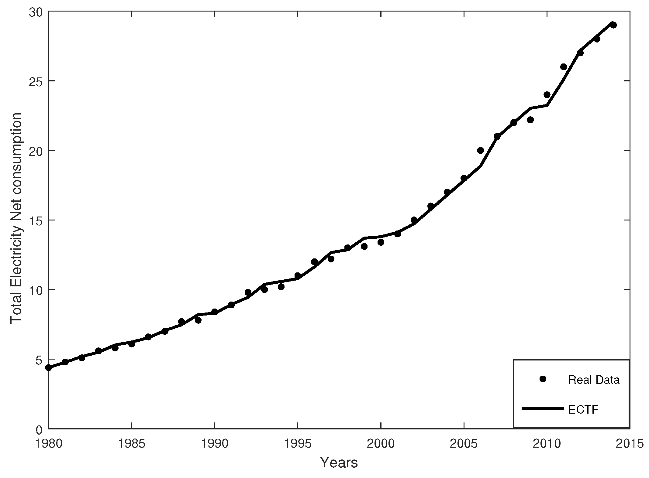
According to Zehna’s theorem [31], the Estimated Trend Function (ETF) and Estimated Conditional Trend Function (ECTF) of the proposed model are obtained by replacing the parameters in Equations (2) and (3) by their estimators given in Equations (6), (7) and (9). Then, the ECTF and ETF have the following expressions:

$$\widehat{\mathbb{E}}(x\left(t\right)\mid x\left(s\right)=x_s)=x_s{e}^{\widehat{\alpha }(t-s)}+\frac{\widehat{\beta }}{\widehat{\alpha }}\left(e^{\widehat{\alpha }(t-s)}-1\right).$$

(15)

Under the initial condition $\mathrm{P}\left(x\left(t_0\right)=x_{t_0}\right)=1$, the trend function of the process is:

$$\widehat{\mathbb{E}}\left(x\left(t\right)\right)=x_{t_0}{e}^{\widehat{\alpha }(t-t_0)}+\frac{\widehat{\beta }}{\widehat{\alpha }}\left(e^{\widehat{\alpha }(t-t_0)}-1\right).$$

(16)

4.3. Approximate Asymptotic Confidence Interval of the Trend Functions

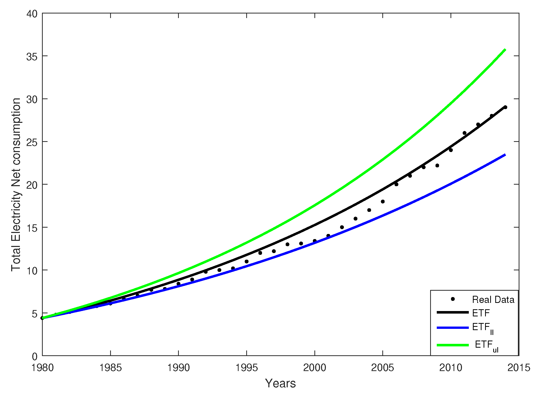
Asymptotic and approximate confidence intervals of the ETF of the model can be obtained by replacing in Equations (2) and (3) the parameters $\alpha$ and $\beta$ by the extreme values of those confidence intervals: the lower limit of $\alpha$ and $\beta$ (${\alpha }_{ll}$ and ${\beta }_{ll}$, respectively) and the upper limit of $\alpha$ and $\beta$ (${\alpha }_{ul}$ and ${\beta }_{ul}$, respectively), which are given in expression Equations (13) and (14). Then, the lower limit of the ETF (${\mathrm{ETF}}_{ll}$) is given by:

$${\widehat{\mathbb{E}}}_{ll}\left(x\left(t\right)\right)=x_{t_0}{e}^{{\widehat{\alpha }}_{ll}(t-t_0)}+\frac{{\widehat{\beta }}_{ll}}{{\widehat{\alpha }}_{ll}}\left(e^{{\widehat{\alpha }}_{ll}(t-t_0)}-1\right),$$

(17)

and the upper limit of the ETF (${\mathrm{ETF}}_{ul}$) is:

$${\widehat{\mathbb{E}}}_{ul}\left(x\left(t\right)\right)=x_{t_0}{e}^{{\widehat{\alpha }}_{ul}(t-t_0)}+\frac{{\widehat{\beta }}_{ul}}{{\widehat{\alpha }}_{ul}}\left(e^{{\widehat{\alpha }}_{ul}(t-t_0)}-1\right).$$

(18)

These functions are utilized in the last section to fit and predict the future evolution of the stochastic diffusion process under consideration.

5. Application and Results

In this application, we examined the variable $x\left(t\right)$ defined by total electricity net consumption expressed in ${10}^9$ kWh in Morocco, such that the total electricity net consumption = total net electricity generation + electricity imports − electricity exports − electricity transmission and distribution losses. Note that the net consumption excludes the energy consumed by the generating units.

Indeed, the analysis of the consumption of electrical energy, as well as other energy products (gas, petroleum products, etc.), represents a complicated problem. This is due to the fact that the consumption intended for the domestic, industrial, agricultural, or other possible sector depends on a large number of variables of different natures (economic, demographic, sociological, geographical, or climatological variables), in other words, depending on the type of consumption of the energy considered.

In this situation, it is difficult, for example, to reach functional models associating energy consumption, in particular electricity, with such a large number of variables. This is because, in many cases, these variables are also dependent on each other by multiple linear and nonlinear regression models or by special econometric models. However, even if this modeling is carried out, its practical utility and its degree of adjustment to the observed data do not guarantee a sufficient level of efficiency of such a model, for example to predict the future evolution of the consumption considered.

One possible way to solve this basic problem of modeling that we want to obtain is to accumulate this large number of variables that influence electricity consumption in a “random effect”. This can be done, on the one hand, by considering a stochastic model to describe the electric consumption in question; on the other hand, by describing this consumption by means of an appropriate stochastic process that “globalizes” or “accumulates” the electric consumption to eliminate the random effect produced by the influence of a large number of variables that affect the evolution of consumption and whose influence cannot be described analytically in the final model.

The methodology used in this work, for the modeling of electricity consumption in the geographical region considered, the “consumption of electricity accumulated in annual periods”, according to a duration of one year, was modeled by a stochastic diffusion process, of the Brennan–Schwartz type, the variable $x(t,\omega )$ defined as the random value of the “total electricity consumption accumulated during the one-year period ending at time t”, where $t\in [0,T]$.

All the data, shown in

Table 1. Fit from 1980–2012.

Years	Data in ${10}^9$ kWh	ETF	ECTF
Observed Values
1980	4.4000	4.4000	4.4000
1981	4.8000	4.7717	4.7717
1982	5.1000	5.1573	5.1867
1983	5.6000	5.5574	5.4979
1984	5.8000	5.9724	6.0167
1985	5.9000	6.4031	6.2242
1986	6.6000	6.4898	6.3279
1987	7.0000	7.1343	7.0542
1988	7.7000	7.7943	7.4662
1989	7.7000	8.2932	8.1954
1990	8.4000	8.8108	8.1954
1991	8.9000	8.3479	8.9216
1992	9.8000	9.9050	9.4404
1993	10.0000	10.4831	10.3741
1994	10.0000	11.0828	10.5816
1995	11.0000	11.7050	10.5816
1996	12.0000	12.3505	11.6191
1997	12.0000	13.0203	12.6566
1998	13.0000	13.7551	12.6566
1999	13.0000	14.4360	13.6941
2000	13.0000	15.1839	13.6941
2001	14.0000	15.9599	13.6941
2002	15.0000	16.7649	14.7316
2003	16.0000	17.6001	15.7691
2004	17.0000	18.4666	16.8065
2005	18.0000	19.3657	17.8815
2006	20.0000	20.2984	18.8440
2007	21.0000	21.2661	20.9565
2008	22.0000	22.2700	21.9940
2009	22.0000	23.3116	23.0315
2010	24.0000	24.3922	23.0315
2011	26.0000	25.5134	25.1064
2012	27.0000	26.6766	27.1814

, are annual and were extracted from the U.S. Energy Information Administration that provides data for Morocco from 1980–2014. The data, available by year and country accessed at: https://www.theglobaleconomy.com/.

Table 1 summarizes the observed values and those estimated for the trend functions, i.e., the ETF and the ECTF, respectively for the corresponding years.

The estimators calculated together with the upper and lower limits of the $95\%$ confidence intervals for the parameters of the drift and the diffusion coefficient of the proposed model are given in

Table 2. Parameters’ estimation and the limits of the $95\%$ confidence intervals.

Parameters’ Estimation	Lower Limit	Upper Limit
$\widehat{\alpha }=0.036802278990569$	$0.031722514789153$	$0.041882043191985$
$\widehat{\beta }=0.202955446503311$	$0.172968793593128$	$0.232942099413494$
$\widehat{{\sigma }^2}=0.056710443868538$	0.054267898965168	0.059152988771908

.

The data corresponding to 2013 and 2014, which were not applied for fitting data, were applied to forecast the future values of the model, with the trend functions and the confidence interval of $95\%$, and are given in

Table 3. Predictions from the trend functions of the proposed model.

Years	Data	${\mathit{ETF}}_{\mathit{ll}}$	ETF	${\mathit{ETF}}_{\mathit{ul}}$	ECTF
2013	28.1167	22.6139	27.8833	34.1191	28.2189
2014	29.1350	23.5185	29.1354	35.8163	29.2564

.

Figure 1 and Figure 2 illustrate the fits and the predictions obtained from the ETF and the ECTF.

5.1. Goodness of Fit of the Model

MAPE and Symmetrical MAPE (SMAPE) were used to compare the prediction accuracy. SMAPE is an average measure of the forecast accuracy across a given forecast horizon, and it provides a global measurement of the goodness of fit. In general, as long as the values of MAPE and SMAPE were small (<10), we concluded that the model was accurate and efficient; see [32]. In addition, some authors have proposed SMAPE as the best performance measure to select among models (see [33]).

We denote by $y_i$ the actual value, by $\widehat{y_i}$ the forecast value, and by n the total number of predictions. These two measures of error are defined as:

MAPE is a measure of prediction accuracy that provides reliability, ease of interpretation, and independence of the units. It is expressed as a percentage and can be defined by the following expression:

$$\mathrm{MAPE}=\frac{1}{n}\sum _{t=1}^n\frac{|\widehat{y_i}-y_i|}{y_i}\times 100.$$

According to Lewis [32], the typical MAPE values and their interpretation are shown in

Table 4. Interpretation of typical MAPE values.

MAPE	Interpretation
<10	Highly-accurate forecasting
20–30	Good forecasting
30–50	Reasonable forecasting
>50	Inaccurate forecasting

:

SMAPE is an accuracy measure based on relative errors. It is used to show that the geometric-mean combination of different forecasts produces a better forecast. It is usually defined by:

$$\mathrm{SMAPE}=\frac{100}{n}\sum _{t=1}^n\frac{|\widehat{y_i}-y_i|}{\left(\right|\widehat{y_i}|+|y_i\left|\right)/2}.$$

After calculating the two measures of error (as shown in

Table 5. Goodness of fit of the model. SMAPE, Symmetrical MAPE.

Measures of Forecasting Accuracy Error	Values
MAPE	0.44115148
SMAPE	0.441732605

), we can conclude that the stochastic BSDP is reliable and efficient.

5.2. The Comparison between the Goodness of Fit of the Stochastic BSDP and the Lognormal Model

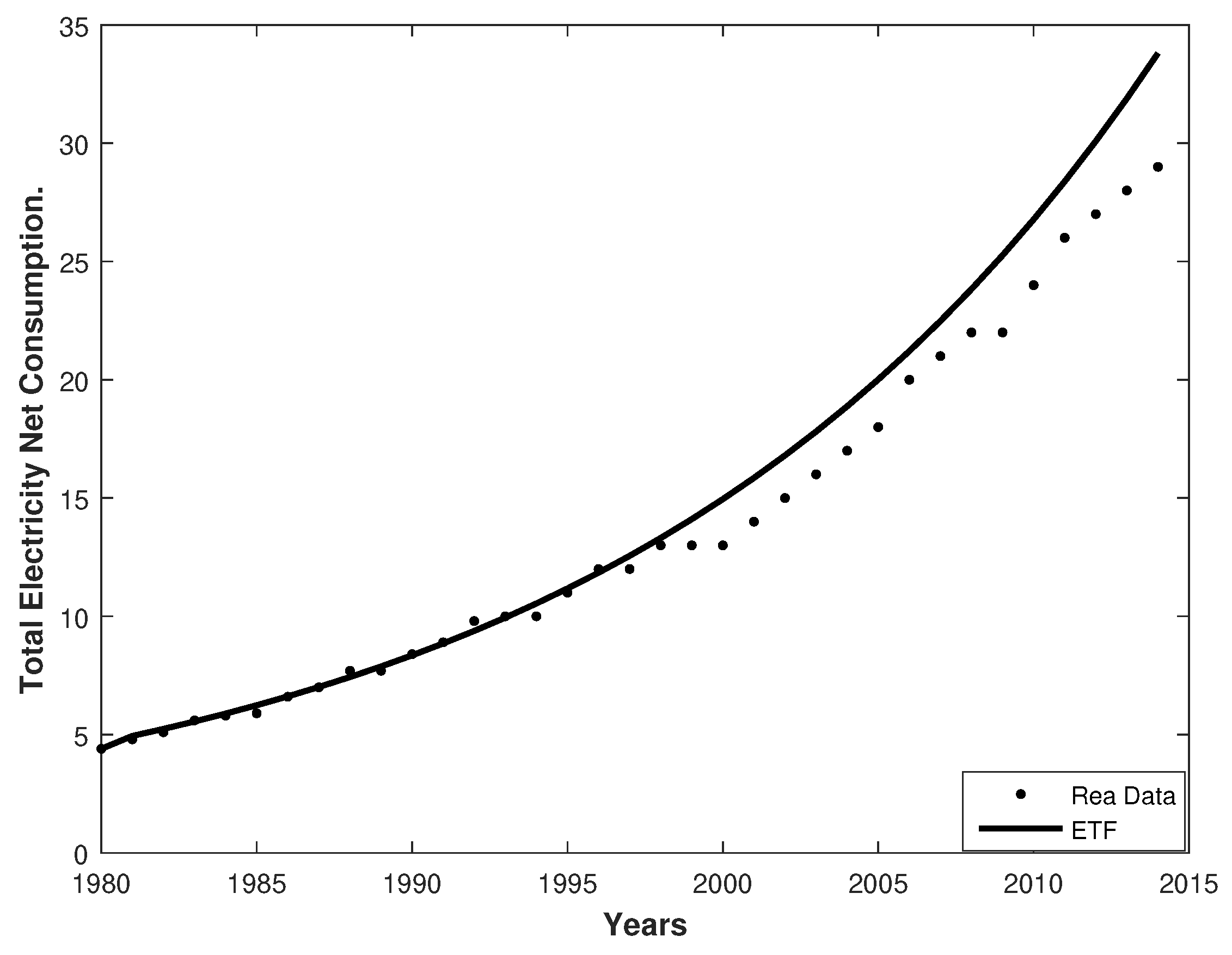
Since the stochastic BSDP is an extension of the stochastic Lognormal Diffusion Process (LDP), we compare, in this section, the MAPE and SMAPE of these two models in order to evaluate the results obtained using the stochastic BSDP in studying our data series (see Appendix C in [4]).

The results obtained using the stochastic BSDP in the data series were compared with those obtained by the stochastic LDP, as shown in the following Figure 3 and Figure 4.

These figures show that the stochastic BSDP was more suitable than the stochastic LDP.

As shown with respect to the stochastic BSDP, the data for the period 2012–2014, which were not used for the statistical fit, were used to forecast the future values of the process.

Table 6. Predictions from trend functions of the stochastic BSDP and LDP processes.

Years	Stochastic BSDP		Stochastic LDP
	Data	ETF	Data	ETF
2013	28.1167	27.8833	31.7717	31.8884
2014	29.1350	29.1354	33.6662	33.8012

shows that the forecasts obtained by the stochastic BSDP for 2012–2014 were better than those obtained by the stochastic LDP.

In our study, the results obtained by the MAPE and the SMAPE as defined in Section 5.1 were compared with those obtained by the stochastic LDP.

We calculated these two measures of error (as shown in

Table 7. Goodness of fit of the two models.

Measures of Forecasting Accuracy Error	Values of BSDP	Values of LDP
MAPE	0.44115148	14.78035099
SMAPE	0.441732605	13.75629617

) and then compared the results with those obtained by the stochastic BSDP.

6. Conclusions

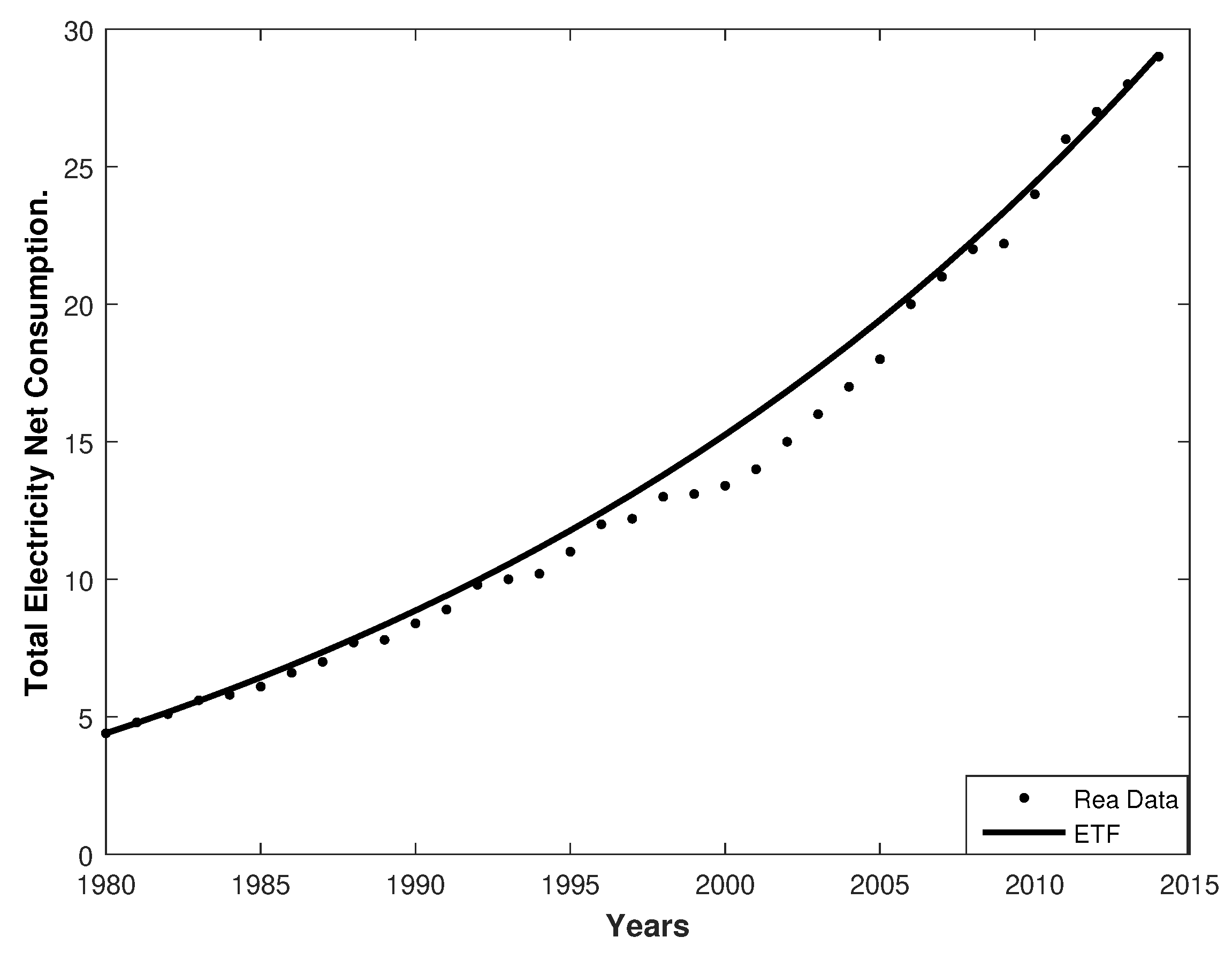
• In this paper, the Brennan–Schwartz diffusion process showed its capability for modeling real data in the field of energy. The proposed methodology was applied to the real case of the evolution of the net consumption of electricity in Morocco and provided a good fit.
• The forecasts and the real data for the period 2013 and 2014 were situated within the confidence interval of the ETF. However, the conditioned trend provided a better accurate fit and forecast than those obtained by the trend alone.
• Finally, by the inclusion of exogenous factors in the process, the fit using ETF could be ameliorated; see for example [11].
• In order to compare the forecasting accuracy of the two models, we calculated two measures of error, MAPE and SMAPE. The values obtained for these two measures of error showed that the stochastic BSDP was more reliable than the stochastic LDP.

References

- Vasicek, O. An equilibrium characterization of the term structure. J. Financ. Econ. 1977, 5, 177–188. [Google Scholar] [CrossRef]
- Brennan, M.J.; Schwartz, E.S. A continuous time approach to the pricing of bonds. J. Bank. Financ. 1979, 3, 133–155. [Google Scholar] [CrossRef]
- Albano, G.; Giorno, V. On Short-Term Loan Interest Rate Models: A First Passage Time Approach. Mathematics 2018, 6, 70. [Google Scholar] [CrossRef]
- Nafidi, A.; Moutabir, G.; Gutiérrez-Sánchez, R.; Ramos-Ábalos, E. Stochastic Square of the Brennan–Schwartz Diffusion Process: Statistical Computation and Application. Methodol. Comput. Appl. Probab. 2019. [Google Scholar] [CrossRef]
- Saha, T.; Chakrabarti, C. Stochastic analysis of prey-predator model with stage structure for prey. J. Appl. Math. Comput. 2011, 35, 195–209. [Google Scholar] [CrossRef]
- Nafidi, A.; Bahij, M.; Achchab, B.; Gutiérrez-Sánchez, R. The stochastic Weibull diffusion process: Computational aspects and simulation. Appl. Math. Comput. 2019, 348, 575–587. [Google Scholar] [CrossRef]
- Di Crescenzo, A.; Paraggio, P. Logistic growth described by birth-death and diffusion processes. Mathematics 2019, 7, 489. [Google Scholar] [CrossRef]
- Gutiérrez, R.; Nafidi, A.; Sánchez, R.G. Forecasting total natural-gas consumption in Spain by using the stochastic Gompertz innovation diffusion model. Appl. Energy 2005, 80, 115–124. [Google Scholar] [CrossRef]
- Skiadas, C.H.; Giovanis, A.N. A stochastic bass innovation diffusion model for studying the growth of electricity consumption in Greece. Appl. Stoch. Models Data Anal. 1997, 13, 85–101. [Google Scholar] [CrossRef]
- Gutiérrez, R.; Gutiérrez-Sánchez, R.; Nafidi, A. Electricity consumption in morocco: Stochastic Gompertz diffusion analysis with exogenous factors. Appl. Energy 2006, 83, 1139–1151. [Google Scholar] [CrossRef]
- Nafidi, A.; Gutiérrez, R.; Gutiérrez-Sánchez, R.; Ramos-Ábalos, E.; El Hachimi, S. Modelling and predicting electricity consumption in spain using the stochastic gamma diffusion process with exogenous factors. Energy 2016, 113, 309–318. [Google Scholar] [CrossRef]
- Bibby, B.M.; Sorensen, M. Martingale estimation functions for discretely observed diffusion processes. Bernoulli 1995, 1, 17–39. [Google Scholar] [CrossRef]
- Kloeden, P.E.; Platen, E. The Numerical Solution of Stochastic Differential Equations; Springer: Berlin, Germany, 1992. [Google Scholar]
- Singer, H. Parameter estimation of nonlinear stochastic differential equations: Simulated maximum likelihood versus extended kalman filter and Itô-taylor expansion. J. Comput. Graph. Stat. 2002, 11, 972–995. [Google Scholar] [CrossRef]
- Prakasa Rao, B. Statistical Inference for Diffusion Type Processes; Arnold: London, UK, 1999. [Google Scholar]
- Courtadon, G. The pricing of options on default-free bonds. J. Financ. Quant. Anal. 1982, 17, 75–100. [Google Scholar] [CrossRef]
- Chan, K.C.; Karolyi, G.A.; Longstaff, F.A.; Sanders, A.B. An empirical comparison of alternative models of the short-term interest rate. J. Financ. 1992, 47, 1209–1227. [Google Scholar] [CrossRef]
- Gutiérrez, R.; Angulo, J.; González, A.; Pérez, R. Inference in lognormal multidimensional diffusion processes with exogenous factors: Application to modeling in economics. Appl. Stoch. Models Data Anal. 1991, 7, 295–316. [Google Scholar] [CrossRef]
- Gutiérrez, R.; Román, P.; Romero, D.; Torres, F. Forecasting for the univariate lognormal diffusion process with exogenous factors. Cybern. Syst. 2003, 34, 709–724. [Google Scholar] [CrossRef]
- Nobile, A.; Ricciardi, L. Growth with regulation in fluctuating environments. Biol. Cybern. 1984, 50, 285–299. [Google Scholar] [CrossRef] [Green Version]
- Nicolau, J. Processes with volatility-induced stationarity: An application for interest rates. Stat. Neerl. 2005, 59, 376–396. [Google Scholar] [CrossRef]
- Gradshteyn, I.S.; Ryzhik, I.M. Table of Integrals, Series, and Products; Academic Press: Cambridge, MA, USA, 1979. [Google Scholar]
- Chesney, M.; Elliott, R.J. Estimating the instantaneous volatility and covariance of risky assets. Appl. Stoch. Models Data Anal. 1995, 11, 51–58. [Google Scholar] [CrossRef]
- Florens-Zmirou, D. Approximate discrete-time schemes for statistics of diffusion processes. Stat. J. Theor. Appl. Stat. 1989, 20, 547–557. [Google Scholar] [CrossRef]
- Yoshida, N. Estimation for diffusion processes from discrete observation. J. Multivar. Anal. 1992, 41, 220–242. [Google Scholar] [CrossRef] [Green Version]
- Kloeden, P.E.; Platen, E.; Schurz, H.; Sorensen, M. On effects of discretization on estimators of drift parameters for diffusion processes. J. Appl. Probab. 1996, 33, 1061–1076. [Google Scholar] [CrossRef]
- Giovanis, A.; Skiadas, C. A stochastic logistic innovation diffusion model studying the electricity consumption in Greece and the United States. Technol. Forecast. Soc. Chang. 1999, 61, 235–246. [Google Scholar] [CrossRef]
- Gutiérrez, R.; Gutiérrez-Sánchez, R.; Nafidi, A. Emissions of greenhouse gases attributable to the activities of the land transport: Modelling and analysis using I–CIR stochastic diffusion the case of Spain. Environmetrics 2008, 19, 137–161. [Google Scholar] [CrossRef]
- Kutoyants, Y.A. Statistical Inference for Ergodic Diffusion Processes; Springer Science and Business Media: Berlin/Heidelberg, Germany, 2004. [Google Scholar]
- Gutiérrez, R.; Gutiérrez-Sánchez, R.; Nafidi, A. Modelling and forecasting vehicle stocks using the trends of stochastic Gompertz diffusion models: The case of Spain. Appl. Stoch. Models Bus. Ind. 2009, 25, 385–405. [Google Scholar] [CrossRef]
- Zehna, P.W. Invariance of maximum likelihood estimators. Ann. Math. Stat. 1966, 37, 744. [Google Scholar] [CrossRef]
- Lewis, C.D. Industrial and Business Forecasting Methods: A Practical Guide to Exponential Smoothing and Curve Fitting; Butterworth-Heinemann: Oxford, UK, 1982. [Google Scholar]
- Makridakis, S.; Hibon, M. The M3-Competition: Results, conclusions and implications. Int. J. Forecast. 2000, 16, 451–476. [Google Scholar] [CrossRef]
Figure 1.
The real data versus those fitted by the Estimated Trend Function (ETF), the , and the .
Figure 2.
The data observed versus those fitted by the Estimated Conditional Trend Function (ECTF).
Figure 3.
The data observed versus those fitted by the stochastic Brennan–Schwartz Diffusion Process (BSDP).
Figure 4.
The real data versus those fitted by the stochastic Lognormal Diffusion Process (LDP).