Efficacy of the Post-Exposure Prophylaxis and of the HIV Latent Reservoir in HIV Infection
by
 , and
, and
Carla M. A. Pinto
1,2,*,† ,
,
Ana R. M. Carvalho
3,†, 
Dumitru Baleanu
4,† and
Hari M. Srivastava
5,6,† 1
School of Engineering, Polytechnic of Porto, Rua Dr António Bernardino de Almeida, 431, 4200-072 Porto, Portugal
2
Centre for Mathematics, University of Porto, Rua do Campo Alegre s/n, 4440-452 Porto, Portugal
3
Faculty of Sciences, University of Porto, Rua do Campo Alegre s/n, 4440-452 Porto, Portugal
4
Department of Mathematics and Computer Sciences, Cankaya University, Balgat, Ankara 0630, Turkey
5
Department of Mathematics and Statistics, University of Victoria, Victoria, BC V8W 3R4, Canada
6
Department of Medical Research, China Medical University Hospital, China Medical University, Taichung 40402, Taiwan
*
Author to whom correspondence should be addressed.
†
The authors contributed equally to this work.
Mathematics 2019, 7(6), 515; https://doi.org/10.3390/math7060515
Submission received: 17 April 2019
/
Revised: 1 June 2019
/
Accepted: 4 June 2019
/
Published: 5 June 2019
(This article belongs to the Special Issue Fractional-Order Integral and Derivative Operators and Their Applications)
Abstract
:We propose a fractional order model to study the efficacy of the Post-Exposure Prophylaxis (PEP) in human immunodeficiency virus (HIV) within-host dynamics, in the presence of the HIV latent reservoir. Latent reservoirs harbor infected cells that contain a transcriptionally silent but reactivatable provirus. The latter constitutes a major difficulty to the eradication of HIV in infected patients. PEP is used as a way to prevent HIV infection after a recent possible exposure to HIV. It consists of the in-take of antiretroviral drugs for, usually, 28 days. In this study, we focus on the dosage and dosage intervals of antiretroviral therapy (ART) during PEP and in the role of the latent reservoir in HIV infected patients. We thus simulate the model for immunologically important parameters concerning the drugs and the fraction of latently infected cells. The results may add important information to clinical practice of HIV infected patients.
1. Introduction
The human immunodeficiency virus (HIV) is a retrovirus, which impairs the host immune system, by destroying preferably the CD4+ T cells. These cells are essential to guarantee immune protection. They do so by helping B cells produce antibodies, inducing macrophages to develop enhanced microbicidal activity, recruiting neutrophils, eosinophils, and basophils to inflammation and infection sites, and, by producing cytokines and chemokines. A number of CD4+ T cells below a given threshold is a synonym of immunodeficiency. The organism is thus vulnerable to a broad set of infections, cancers and other diseases.
HIV occurs in two types: HIV-1 and HIV-2, and is transmitted by the exchange of HIV-infected body fluids, such as blood, semen, and genital secretions. It may also be transmitted from an HIV-infected pregnant woman to her child, during pregnancy, birth, or breastfeeding [1].
HIV is a defying global health threat, responsible for more than 36.7 million infected people worldwide, and more than 35 million deaths, so far. In 2016, the number of deceased from HIV-related causes was estimated at one million. Figures are even more striking since, globally, 1.8 million people become newly infected each year. Access to antiretroviral therapy is crucial to control the virus and to reduce the risk of transmission, providing HIV infected individuals and those at risk, more healthy, long and productive lives. In 2016, nearly half of the adults and children living with HIV had access to treatment. Effective treatment reduces the risk of HIV transmission to non-infected sexual partners by 96% [2]. Other forms of HIV prevention are the Pre-Exposure Prophylaxis (PrEP) and the Post-Exposure Prophylaxis (PEP).
PrEP is the daily in-take of ART to prevent HIV infection in uninfected people. The usual combination of the two HIV drugs, tenofovir and emtricitabine, sold under the name of Truvada, is approved for daily use as PrEP. PrEP is shown to be highly effective for HIV prevention, when taken consistently. WHO recommends PrEP as one of the prevention options, for people at substantial risk of HIV infection (namely injecting drug users, men who have sex with men, and high-risk heterosexual couples), and for HIV-negative women who are pregnant or breastfeeding [2].
PEP consists of the intake of ART, after possible exposure to HIV. It includes counseling, first aid care, HIV testing, and administration of a 28-day course of ART with follow-up care. It is intended to prevent HIV spread in the human body, protecting against being re-exposed to HIV and reducing the chances of HIV transmission [3]. PEP was initially intended for healthcare workers, who had been accidentally exposed to HIV-infected body fluids, through injury with a contaminated syringe, etc. Nowadays, WHO recommends PEP for both health-worker and non-health-workers, for adults and children [2]. PEP should be started immediately after exposure and at most 72 hours after, to enhance the rate of success, since it is not 100% effective [3].
Latent reservoirs consist of a small proportion of resting CD4+ T cells, containing integrated proviral DNA [4,5,6]. Latent reservoirs are established during the acute phase of HIV infection. These reservoirs may hide out for years in many tissues in the body, namely lymph nodes, seminal fluid, and cerebral spinal fluid. Latent reservoirs can, however, wake up, and release old viral variants in the blood. The mechanism behind this activation is summarized as follows. Proviral genomes are integrated in resting memory CD4+ T cells. Due to the quiescent state of these latent cells, these genomes are not transcribed into mRNA (messenger ribonucleic acid) and translated in protein to become active virus. Nevertheless, when cell activation occurs, then transcription and translation may recommence [7]. This affects the viral dynamics of untreated patients, promoting viral load rebounds. ART can suppress HIV load levels to undetectable values, however, it cannot eliminate the latent reservoir. This is the main challenge to HIV cure.
Considerable research has been found in the literature to describe the effects of HIV prevention strategies. In 2009, Lou et al. [8] study drug dynamics, drug dosages, and therapy strategies in an impulsive model for the dynamics of HIV in the presence of PEP. Authors conclude that the best choice for an infected individual is a safe dose of medication during PEP. Moreover, the side effects of ART should also be taken into consideration in choosing the appropriate therapy. Conway et al. [9] present a stochastic model for the dynamics of HIV, immediately after exposure, and apply drug prophylaxis to understand how it reduces the risk of infection. The authors predict that a two-week PEP regimen may be as effective as the recommended four-week treatment protocol. In 2014, Kim et al. [10] study a model for HIV infection in men who have sex with men (MSM) in South Korea. They simulate the effects of early ART, early diagnosis, PrEP, and combination interventions, on the incidence and prevalence of HIV infection. The authors conclude that PrEP and early diagnosis would be effective ways in reducing HIV incidence in MSM. In 2017, Pinto et al. [11], evaluate the impact of PrEP and screening in the dynamics of HIV in infected patients. The proposed model incorporates condom use, the number of sexual partners, and treatment for HIV. The basic reproduction number is extremely impacted by the efficacy of the screening, pointing to explicit campaigns highlighting screening. The results from the model are fitted to data on the cumulative HIV and AIDS (acquired immunodeficiency syndrome) cases in Portugal.
Fractional Calculus—Short Recap
Fractional Calculus has been a hot research topic in the last few decades. Researchers from distinct scientific areas, theoretical and applied, have studied fractional order models to obtain a deeper understanding of real world phenomena [4,12,13,14,15,16,17]. Fractional order models are characterized by a ‘memory’ property, which brings additional information to analyze the systems’ dynamical behaviors.
The classical definitions for a derivative of fractional (non-integer) order are the Caputo (C), the Riemann-Liouville (RL) and the Grünwald-Letnikov (GL). Let be the interval, instead of , for simplification. The function is smooth in every interval , The RL definition reads:
where is the Euler Gamma function. The Caputo definition is given by:
The GL definition is based on finite differences and is equivalent to the RL formula:
The memory effect in biology/epidemiology/immunology is extremely important, thus the appearance of fractional order models in the study of patterns arising in these models comes as a natural generalization of the integer order models [18,19,20,21]. In [20], the authors generalize an integer order model for HIV dynamics to include a fractional order derivative. In Arafa et al. [18] the authors generalize an integer order model for HIV dynamics to include a fractional order derivative. They conclude that the fractional order model provides a better fit to real data from 10 patients than the integer order model. Pinto [4] studies the role of the latent reservoir in the persistence of the latent reservoir and of the plasma viremia in a fractional-order (FO) model for HIV infection. The model assumes that (i) the latently infected cells may undergo bystander proliferation, without active viral production, (ii) the latent cell activation rate decreases with time on ART, and (iii) the productively infected cells’ death rate is a function of the infected cell density. The model clarifies the role of the latent reservoir in the persistence of the latent reservoir and of the plasma virus. The non-integer order derivative is associated with distinct velocities in the dynamics of the latent reservoir and of plasma virus. In [12], the authors study the effect of the HIV viral load in a coinfection fractional order model for HIV and HCV (hepatitis C virus) coinfection. HIV has a significant impact on the burden of the coinfection. Moreover, the order of the fractional derivative may pave the way to a better understanding of the individuals’ compliance to treatment, the distinct responses of the immune system. The non-integer order derivative adds another degree of freedom to the model. In what concerns drug diffusion in tissues, there are some interesting results in the literature. In [22], the authors propose non-integer order (fractional order) models to represent anomalous diffusion, memory effects and power-law clearance rates, typical of drug uptake and diffusion in a case-study of a drug used for cancer therapy. They conclude that fractional models avoid unbounded accumulation of drugs, seen in the integer order approach, and help to prevent life-threatening side-effects on patients. In 2017 [23], the authors provide a review on pharmacokinetic models and propose their generalizations to fractional orders. The new models account for tissue trapping as well as short- and long-time recirculating effects. The benefits from such approach are twofold: (i) a better understanding of secondary effects on patients under treatment; and (ii) avoidance of unbounded drug accumulation.
With the aforementioned ideas in mind, we outline the paper as follows. In Section 2, we describe the proposed model. We follow with the computation of the reproductive number and the stability of the disease free equilibrium in Section 3. Then, in Section 4, we prove the global stability of the disease free equilibrium. The model is simulated and the corresponding results are discussed in Section 5. Finally, in Section 6, we conclude this work.
2. The Model
The model consists of seven classes: the healthy and susceptible CD4+ T cells, T, the healthy and non-susceptible CD4+ T cells, , the latently infected CD4+ T cells, L, the infected and infectious CD4+ T cells, I, the infected and non-infectious CD4+ T cells, , the HIV virus, V, and the drug concentration in the plasma, R.
CD4+ T cells are produced with rate and die with rate . These cells are infected by HIV and by infected CD4+ T cells at rates and , respectively. The healthy T cells are inhibited by drug at rate q. A fraction, , of infected CD4+ T cells becomes latently infected. The latently infected CD4+ T cells become productively infected at a rate and die with a rate . The infected CD4+ T cells die with rate a and are inhibited by drug at rate p. The virus are produced by infected CD4+ T cells at rate k and cleared at rate c. The dynamics of the drugs is as follows. For simplicity, we postulate that after taking the drug, the cell, , inhibits infection until it dies. We further assume that drugs are taken at times , and their effect is instantaneous. The latter results in a system of impulsive differential equations, with condition , where is the dosage. For , the solutions are continuous and obey system (1). The drug, R, is cleared at rate g.
The nonlinear system of fractional differential equations describing the model is given by:
where the parameter is the order of the fractional derivative. The fractional derivative of the proposed model is used in the Caputo sense.
3. Reproduction Number
In this section, we compute the reproduction number of model (1) in the cases of no drug, , and of drug therapy, , and the local stability of its disease-free equilibrium. The basic reproduction number is defined as the number of secondary CD4+ T cells infections due to a single infected cell in a completely susceptible population. We start with . We use the next generation method [24].
The disease-free equilibrium of model (1) is given by:
Using the notation in [24] on system (1), matrices for the new infection terms, , and the other terms, , are given as follows. The chosen variables of the model are L, I and V and the procedure is identical to [24].
The associative basic reproduction number is written as:
where indicates the spectral radius of . The local stability of can be determined using Lemmas 1 and 2.
Lemma 1.
Lemma 2.
The disease-free equilibrium of the system (1) is unstable if .
Proof.
Let be given by:
Expanding, , where is the identity matrix, we have the following equation in terms of :
Now, the arguments of the roots of the equation, , are given by:
where .
Using Descartes’ rule of signs, we find that there is exactly one sign change of the equation:
for . Thus, there is exactly one positive real root of the aforesaid equation for which the argument is less than . As such, we conclude that if the disease-free equilibrium of the system (1) is unstable. □
Now, we discuss the dynamics of system (1) with drugs. The disease-free equilibrium of model (1) with drugs is given by:
Using the notation in [24] on system (1), matrices for the new infection terms, , and the other terms, , are given by:
In this case, the basic reproduction number is computed to be:
where indicates the spectral radius of . The stability of disease-free equilibrium in the case of the drug therapy, , can be determined using the following lemmas:
Lemma 3.
Lemma 4.
The disease-free equilibrium of the system (1) is unstable if .
Proof.
Let be given by:
Expanding, , where is the identity matrix, we have the following equation in terms of :
Now, the arguments of the roots of the equation, , , , and , are given by:
where .
Using Descartes’ rule of signs, we find that there is exactly one sign change of the equation:
for . Thus, there is exactly one positive real root of the aforesaid equation for which the argument is less than . As such, we conclude that, if , the disease-free equilibrium of the system (1) is unstable. □
4. Global Stability of the Disease-Free Equilibrium
In this section, we compute the global stability of the disease-free equilibrium of the model (1). Following Castillo & Chavéz [26], we rewrite model (1) as:
where and , with being the number of uninfected and non-susceptible CD4+ T cells and drugs, and denoting the number of latent and infected CD4+ T cells, virus, and non-infectious CD4+ T cells.
The disease-free equilibrium is written as , where .
The conditions and must be met to guarantee the global asymptotic stability of the disease-free equilibrium of the model (1):
where can be written in the form , where () and is a diagonal matrix. is the region where the model makes biological sense. If the system (10) satisfies the conditions in (11) the following theorem holds [26].
Theorem 1.
Proof.
Let
and
and
All conditions are satisfied, thus is globally asymptotically stable. □
5. Numerical Results
We simulate the model (1) for different values of the order of the fractional derivative, and for clinically relevant parameters. We have applied the Predictor–Evaluator–Corrector–Evaluator PECE method of Adams–Bashford–Moulton type [27]. The parameters used in the simulations, based on [8,28], are: L day, day, day, day, day, day, day, M day, M day, day, , day, day, , day, and the initial conditions are: , , and .
In Figure 1 and Figure 2, we consider model (1) without PEP, for different values of the order of the fractional derivative, . The concentration of CD4+ T cells decreases over time and with . This suggests that the infection is more severe as is lowered. This pattern is supported by the graphs in Figure 2, where it is observed a ratio of healthy T cells to total T cells starting with for , and decreasing for and . Moreover, this ratio points to chronic infection, as the disease evolves, for all .
In Figure 3 and Figure 4, we plot the dynamics of the drug R and of the basic reproduction number , for different values of the order of the fractional derivative, . These figures show that the dosage of the drug is important for controlling HIV infection, since varies with R. As R increases, smaller values of are observed, which indicate less infection. Moreover, the value of the fractional derivative, , may also contribute to controlling the severity of the infection, since smaller values of are observed with decreasing .
Figure 5 depicts the HIV viral load for a dosage and dosing interval day, for different values of the order of the fractional derivative, . As it is shown, the dosage of the drug and the dosing interval are sufficient to control the infection, with the viral load going asymptotically to zero. Similar patterns are seen for all values of , with higher initial viral load for smaller , but faster velocity of convergence.
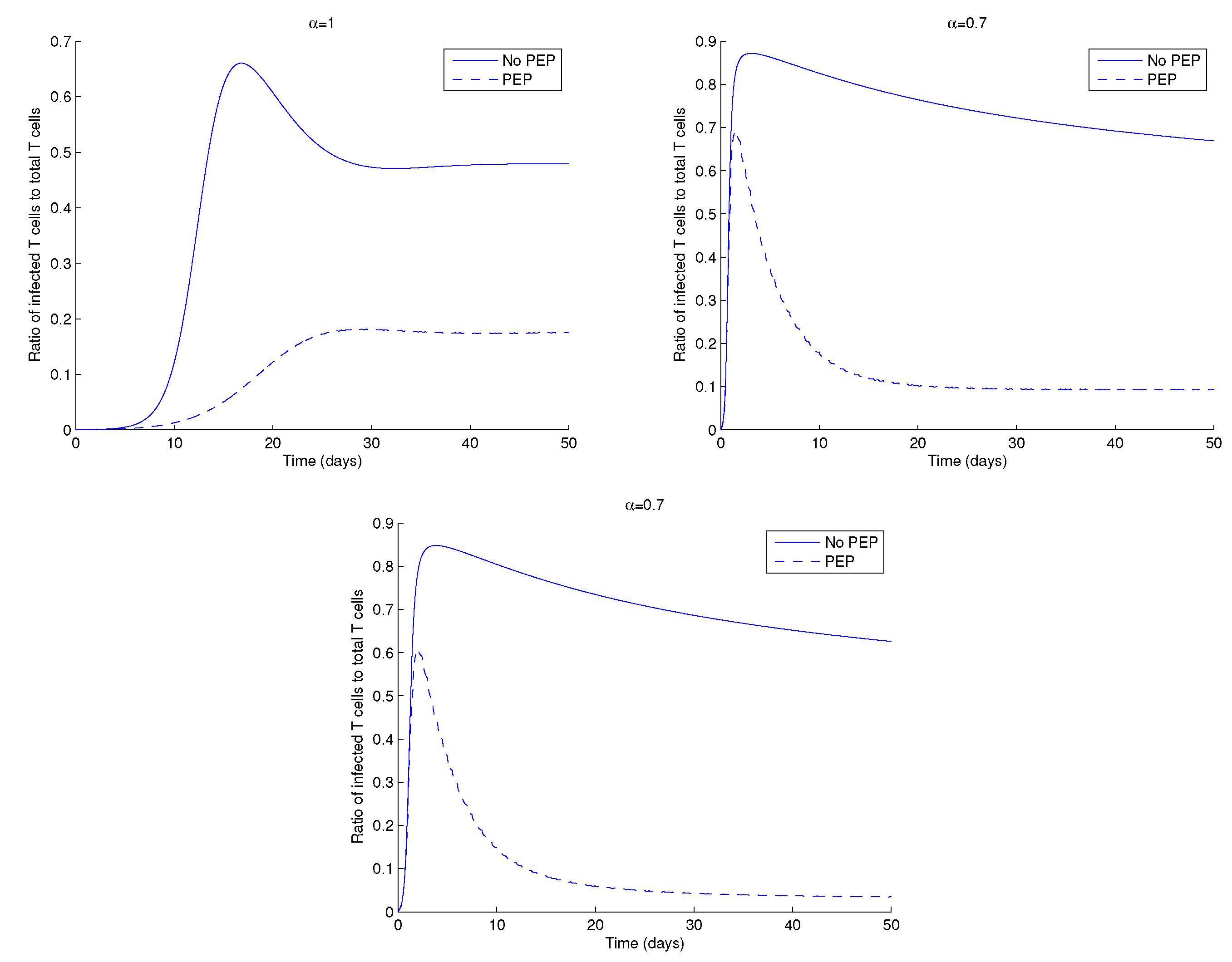
Figure 6 shows the ratio of the infected CD4+ T cells to total CD4+ T cells in the presence and absence of PEP, with low drug dosage, for different values of the order of the fractional derivative, . The ratio of infected to total CD4+ T cells is always smaller when patients are under PEP, when compared to the case without treatment.
In the next figures, we study the effect of different treatment strategies in the dynamics of HIV. We start in Figure 7 with two different treatment strategies: drug perfect adherence and drug therapy breaks. The last strategy consists of intervals (days) in which the therapy is stopped () followed by intervals where there is perfect drug adherence. Perfect adherence therapy consists of taking a dosage for all . In Figure 7, the drug therapy breaks consist of stopping drug application for two days, followed by drug perfect adherence strategy for five days. It is observed that the elimination of HIV from the body takes longer for drug therapy breaks. This is seen for all . Moreover, despite a higher initial peak, the asymptotic HIV viral load is reached faster for smaller .
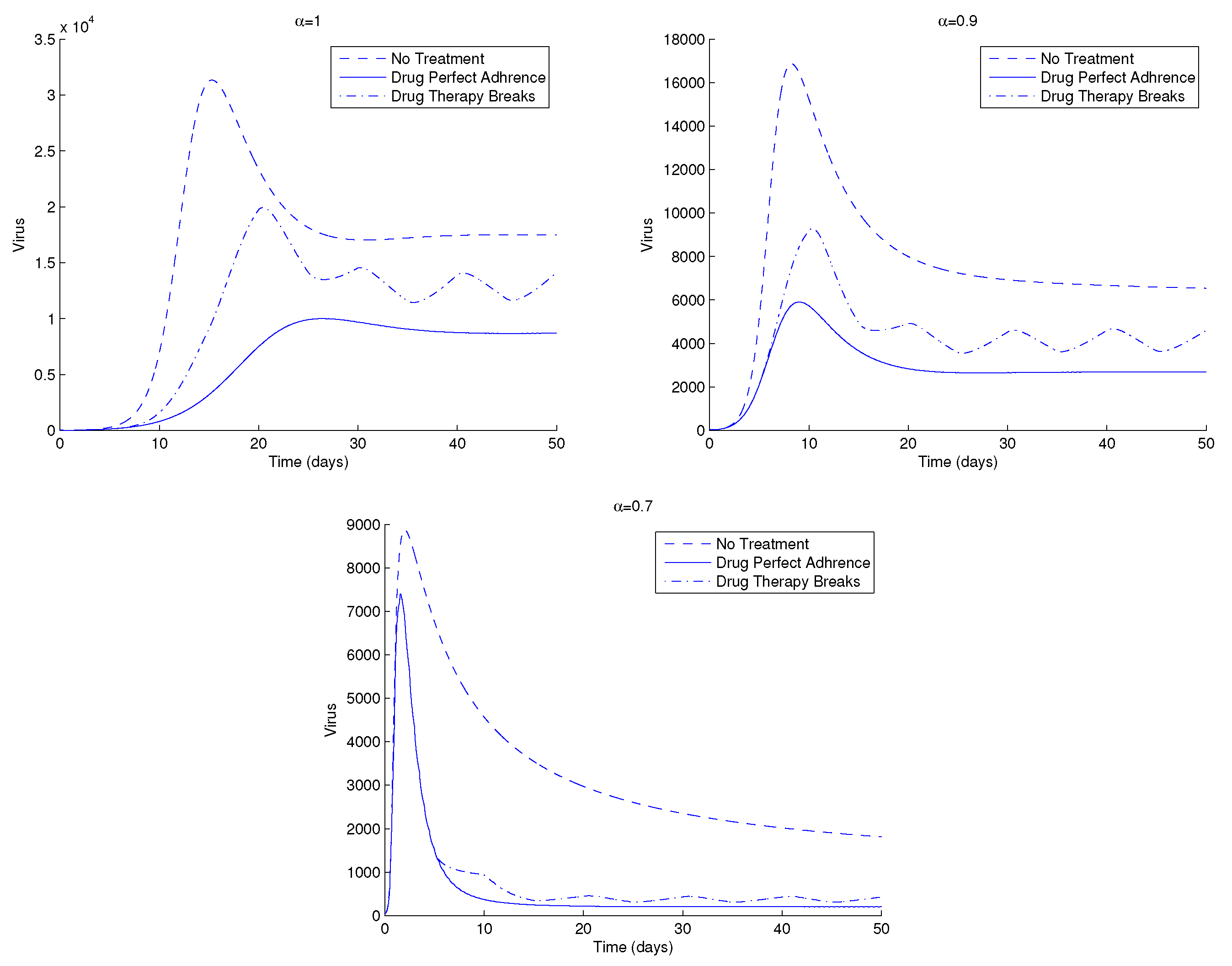
Figure 8 shows another example of the dynamics of the HIV, this time for three distinct treatment strategies: without treatment, drug perfect adherence, and drug therapy breaks. The intervals for the drug therapy breaks are in this case as follows. Five days of no drug administration, which are followed by five more days of perfect drug adherence strategy. The model provides oscillating solutions for the case of drug therapy breaks, as is seen in the figure.
In Figure 9 we show the dynamics of HIV for increasing values of the cell to cell transmission rate, , for three treatment strategies: no treatment, drug perfect adherence and drug therapy breaks, and for varying . The drug therapy breaks strategy stops drug application for 15 days, followed by another 15 days of perfect drug adherence strategy. We observe higher peaks of the viral load and the corresponding curve, in the case of drug therapy breaks, is between the curves of no treatment and drug perfect adherence. This behaviour is repeated for all .
The simulations of the model reveal that a combination of sufficient drug dosage and drug frequency may induce better efficacy of PEP. Drug perfect adherence strategy is always better than the other two. Nevertheless, one must think about the side effects of ART, though their toxicity has been reduced as medicine evolves and new treatment options appear.
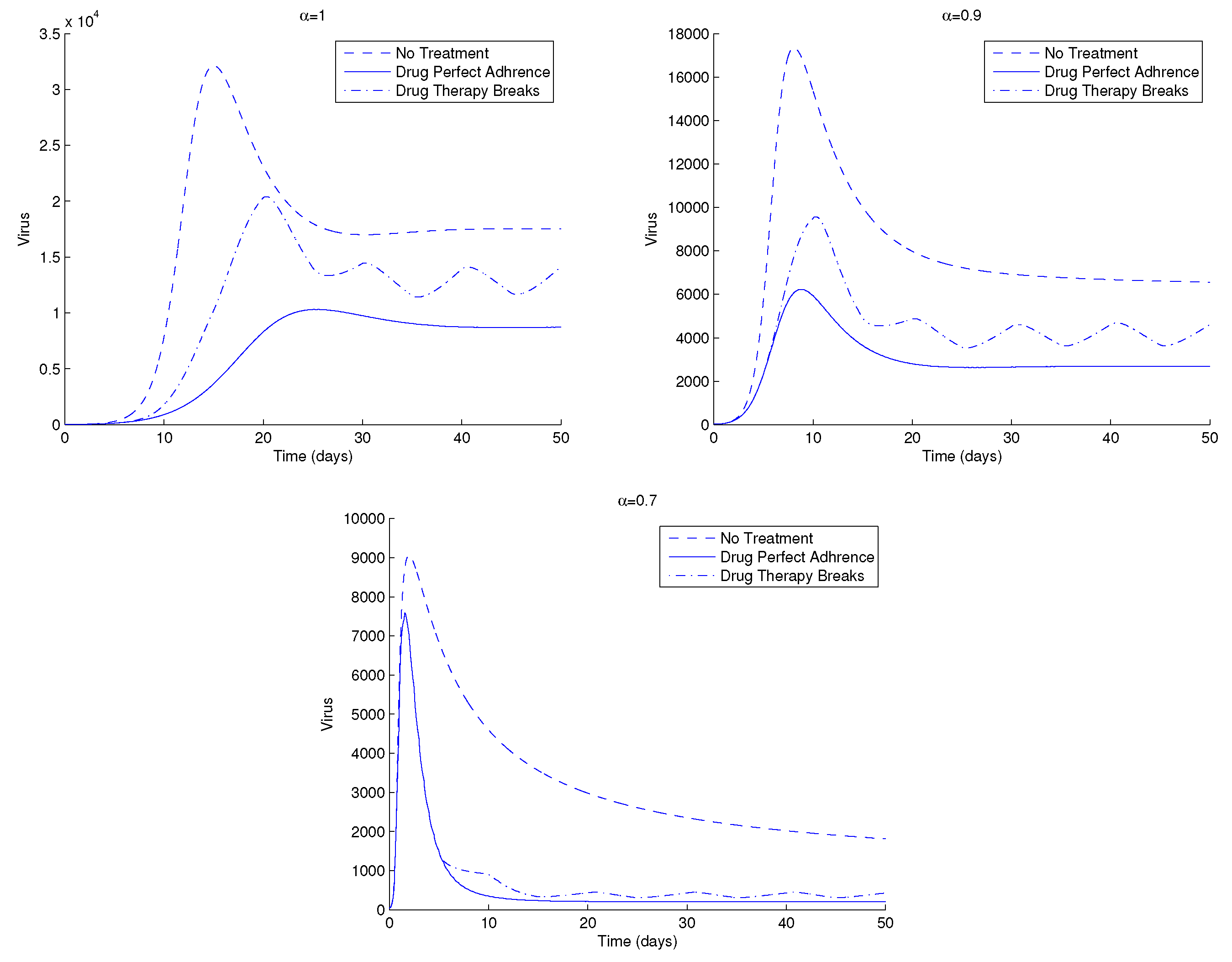
We now proceed with the simulation of the effect of the latent reservoir in the dynamics of HIV infection, under the conditions of Figure 8. We consider three treatment strategies: without treatment, drug perfect adherence, and drug therapy breaks. The intervals for the drug therapy breaks consist of 10 days. In the first five days, the drug is halted, whereas for the last five days, the perfect drug adherence strategy is applied. The difference from Figure 8 is in the value of , which represents the proportion of latently infected CD4+ T cells. The value of is reduced from to . Figure 10 shows slight higher peaks of HIV for , in particular, for smaller values of .
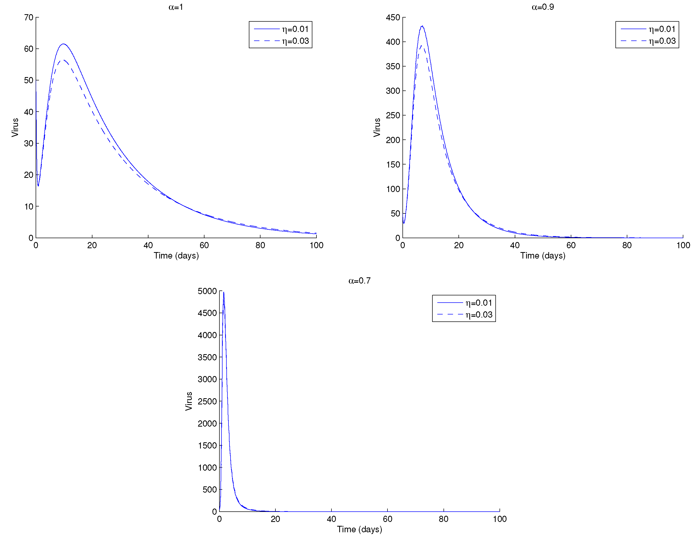
In Figure 11, we plot the viral load for two values of , the fraction of latent infected cells. We note that the asymptotic value of the virus is the same for all . Nevertheless, there are subtle changes in the dynamics of the virus. In the transient are observed smaller values of HIV viral load for , whereas in the asymptotic value there is a switch in this behaviour, and higher values of HIV are seen for . This may be explained as follows. When , there are more latently infected cells in the body. If these cells encounter an antigen or are exposed to specific cytokines or chemokines, they become actively infected by proviral transcription. The latter causes viral rebound if a patient stops ART. This happens earlier for smaller values of .
6. Conclusions
We propose a model to study the effect of PEP and of the latent reservoir in the dynamics of HIV infection. We find that specific dosages and intervals are extremely important to control the infection. Moreover, we find that the latent reservoir may influence the dynamics of HIV, though slightly. This is understandable from a clinical point of view since the effect of the latent reservoir takes time to be felt and PEP is considered only in the first 28 days after exposure. After that, the person must be evaluated clinically to assess the adequacy of the treatment. The order of the fractional derivative, , seems to help control the infection in the presence of PEP and increases the severity of infection when there is no PEP. We observe a somewhat ‘synergistic’ relation between PEP and . The FO derivative may also help to distinguish other traits (age, immune system response, genetic profile), and this may help to devise better therapeutic regimens, that could improve patients’ quality of life, either by diminishing the burden of the therapy or increasing the life span. Moreover, since HIV anti-retroviral therapy (ART) is extremely expensive, an ‘optimal’ (in the sense of more adjusted to each patient) therapy could also imply a reduction in the economic burden of HIV, especially in poor countries, such as the ones included in sub-Saharan Africa. Future work will focus on deepening these and other issues arising from the model.
Author Contributions
All authors contributed equally to the work reported.
Acknowledgments
The authors were partially funded by the European Regional Development Fund through the program COMPETE and by the Portuguese Government through the FCT - Fundação para a Ciência e a Tecnologia under the project PEst-C/MAT/UI0144/2013. The research of AC was partially supported by an FCT grant with reference SFRH/BD/96816/2013.
Conflicts of Interest
The authors declare no conflict of interest.
References
- CDC HIV among Pregnant Women, Infants, and Children. Available online: https://www.cdc.gov/hiv/group/gender/pregnantwomen/index.html (accessed on 2 April 2019).
- WHO. Available online: http://www.who.int/mediacentre/factsheets/fs360/en/ (accessed on 2 April 2019).
- CDCP. Available online: https://www.cdc.gov/hiv/basics/pep.html (accessed on 2 April 2019).
- Pinto, C.M.A. Persistence of low levels of plasma viremia and of the latent reservoir in patients under ART: A fractional-order approach. Commun. Nonlinear Sci. Numer. Simul. 2017, 43, 251–260. [Google Scholar] [CrossRef]
- Rong, L.; Perelson, A.S. Modeling HIV persistence, the latent reservoir, and viral blips. J. Theor. Biol. 2009, 260, 308–331. [Google Scholar] [CrossRef] [PubMed] [Green Version]
- Rong, L.; Perelson, A.S. Modeling latently infected cell activation: Viral and latent reservoir persistence, and viral blips in HIV-infected patients on potent therapy. PLoS Comput. Biol. 2009, 5, e1000533. [Google Scholar] [CrossRef] [PubMed]
- Hill, A.L.; Rosenbloom, D.I.S.; Nowak, M.A.; Siliciano, R.F. Insight into treatment of HIV infection from viral dynamics models. Immunol. Rev. 2018, 285, 9–25. [Google Scholar] [CrossRef] [PubMed]
- Lou, J.; Chen, L.; Ruggeri, T. An impulsive differential model on post exposure prophylaxis to HIV-1 exposed individual. J. Biol. Syst. 2009, 17, 659–683. [Google Scholar] [CrossRef]
- Conway, J.M.; Konrad, B.P.; Coombs, D. Stochastic analysis of Pre- and Postexposure prophylaxis against HIV infection. SIAM J. Appl. Math. 2013, 73, 904–928. [Google Scholar] [CrossRef]
- Kim, S.B.; Yoon, M.; Ku, N.S.; Kim, M.H.; Song, J.E.; Ahn, J.Y.; Jeong, S.J.; Kim, C.; Kwon, H.D.; Lee, J.; et al. Mathematical Modeling of HIV Prevention Measures Including Pre-Exposure Prophylaxis on HIV Incidence in South Korea. PLoS ONE 2014, 9, e90080. [Google Scholar] [CrossRef] [PubMed]
- Pinto, C.M.A.; Carvalho, A.R.M. The impact of pre-exposure prophylaxis (PrEP) and screening on the dynamics of HIV. J. Comput. Appl. Math. 2018, 339, 231–244. [Google Scholar] [CrossRef]
- Carvalho, A.R.M.; Pinto, C.M.A.; Baleanu, D. HIV/HCV coinfection model: A fractional-order perspective for the effect of the HIV viral load. Adv. Differ. Equat. 2018, 2018, 1–22. [Google Scholar]
- Kilbas, A.A.; Srivastava, H.M.; Trujillo, J.J. Theory and Applications of Fractional Differential Equations, North-Holland Mathematical Studies; Elsevier (North-Holland) Science Publishers: Amsterdam, The Netherlands, 2006; Volume 204. [Google Scholar]
- Pinto, C.M.A.; Carvalho, A.R.M. Fractional complex-order model for HIV infection with drug resistance during therapy. J. Vib. Control 2016, 22, 2222–2239. [Google Scholar] [CrossRef]
- Samko, S.; Kilbas, A.; Marichev, O. Fractional Integrals and Derivatives: Theory and Applications; Gordon and Breach Science Publishers: London, UK, 1993. [Google Scholar]
- Sweilam, N.H.; Abou Hasan, M.M.; Baleanu, D. New studies for general fractional financial models of awareness and trial advertising decisions. Chaos Solitons Fractals 2017, 104, 772–784. [Google Scholar] [CrossRef]
- Téjado, I.; Valério, D.; Pérez, E.; Valério, N. Fractional calculus in economic growth modelling: The Spanish and Portuguese cases. Int. J. Dyn. Control 2017, 5, 208–222. [Google Scholar] [CrossRef]
- Arafa, A.A.M.; Rida, S.Z.; Khalil, M. A fractional-order model of HIV infection: Numerical solution and comparisons with data of patients. Int. J. Biomath. 2014, 7, 1450036. [Google Scholar] [CrossRef]
- Arafa, A.A.M.; Rida, S.Z.; Khalil, M. Fractional modeling dynamics of HIV and CD4+ T-cells during primary infection. Nonlinear Biomed. Phys. 2012, 6, 1. [Google Scholar] [CrossRef] [PubMed]
- Ding, Y.; Ye, H. A fractional-order differential equation model of HIV infection of CD4+ T-cells. Math. Comput. Model. 2009, 50, 386–392. [Google Scholar] [CrossRef]
- Yan, Y.; Kou, C. Stability analysis for a fractional differential model of HIV infection of CD4+ T-cells with time delay. Math. Comput. Simul. 2012, 82, 1572–1585. [Google Scholar] [CrossRef]
- Ionescu, C.; Copot, D.; De Keyser, R. Modelling Doxorubicin effect in various cancer therapies by means of fractional calculus. In Proceedings of the 2016 American Control Conference (ACC), Boston, MA, USA, 6–8 July 2016; pp. 1283–1288. [Google Scholar]
- Copot, D.; Magin, R.L.; De Keyser, R.; Ionescu, C. Data-driven modelling of drug tissue trapping using anomalous kinetics. Chaos Solitons Fractals 2017, 102, 441–446. [Google Scholar] [CrossRef]
- Driessche, P.; Watmough, P. Reproduction numbers and sub-threshold endemic equilibria for compartmental models of disease transmission. Math. Biosci. 2002, 180, 29–48. [Google Scholar] [CrossRef]
- Matignon, D. Stability results for fractional differential equations with applications to control processing. Comput. Eng. Syst. Appl. 1996, 2, 963–968. [Google Scholar]
- Castillo-Chavez, C.; Feng, Z.; Huang, W. On the computation of Ro and its role on global stability. In Mathematical Approaches for Emerging and Reemerging Infectious Diseases: An Introduction; Kassem, T., Roudenko, S., Castillo-Chavez, C., Eds.; Springer: New York, NY, USA, 2002. [Google Scholar]
- Diethelm, K.; Freed, A.D. The Frac PECE subroutine for the numerical solution of differential equations of fractional order. In Forschung und Wissenschaftliches Rechnen 1998; Heinzel, S., Plesser, T., Eds.; Gessellschaft fur Wissenschaftliche Datenverarbeitung: Gottingen, Germany, 1999; pp. 57–71. [Google Scholar]
- Hadjiandreou, M.M.; Conejeros, R.; Wilson, D.I. Long-term HIV dynamics subject to continuous therapy and structured treatment interruptions. Chem. Eng. Sci. 2009, 64, 1600–1617. [Google Scholar] [CrossRef]
Figure 1.
Dynamics of the CD T cells, T, of system (1) without PEP for (top left), (top right) and (bottom). Parameter values and initial conditions in the text.
Figure 1.
Dynamics of the CD T cells, T, of system (1) without PEP for (top left), (top right) and (bottom). Parameter values and initial conditions in the text.

Figure 2.
Ratio of healthy CD T cells, T, to total CD T cells, , of system (1) without PEP for (top left), (top right) and (bottom). Parameter values and initial conditions in the text.
Figure 2.
Ratio of healthy CD T cells, T, to total CD T cells, , of system (1) without PEP for (top left), (top right) and (bottom). Parameter values and initial conditions in the text.

Figure 3.
Drug concentration in the plasma, R, given by system (1) for (top left), (top right) and (bottom). Parameter values and initial conditions in the text.
Figure 3.
Drug concentration in the plasma, R, given by system (1) for (top left), (top right) and (bottom). Parameter values and initial conditions in the text.

Figure 4.
Basic reproduction number of system (1) for (top left), (top right) and (bottom). Parameter values and initial conditions in the text.
Figure 4.
Basic reproduction number of system (1) for (top left), (top right) and (bottom). Parameter values and initial conditions in the text.

Figure 5.
HIV viral-load, V, of the system (1) for (top left), (top right) and (bottom). Parameter values and initial conditions in the text, except .
Figure 5.
HIV viral-load, V, of the system (1) for (top left), (top right) and (bottom). Parameter values and initial conditions in the text, except .

Figure 6.
Ratio of infected CD T cells, , to total CD T cells, of system (1) for (top left), (top right) and (bottom). Parameter values and initial conditions in the text, except .
Figure 6.
Ratio of infected CD T cells, , to total CD T cells, of system (1) for (top left), (top right) and (bottom). Parameter values and initial conditions in the text, except .

Figure 7.
HIV viral load of system (1) for two different therapy strategies and (top left), (top right) and (bottom). Parameter values and initial conditions are in the text, except . For more information, see text.
Figure 7.
HIV viral load of system (1) for two different therapy strategies and (top left), (top right) and (bottom). Parameter values and initial conditions are in the text, except . For more information, see text.

Figure 8.
HIV, viral load, V, of system (1) for three different therapy strategies and for (top left), (top right) and (bottom). Parameter values and initial conditions in the text, except . For more information, see text.
Figure 8.
HIV, viral load, V, of system (1) for three different therapy strategies and for (top left), (top right) and (bottom). Parameter values and initial conditions in the text, except . For more information, see text.

Figure 9.
HIV, viral load, V, of system (1) for three different therapy strategies and for (top left), (top right) and (bottom). Parameter values and initial conditions in the text, except and .
Figure 9.
HIV, viral load, V, of system (1) for three different therapy strategies and for (top left), (top right) and (bottom). Parameter values and initial conditions in the text, except and .

Figure 10.
HIV, viral load, V, of system (1) for different therapy strategies and for (top left), (top right) and (bottom). Parameter values and initial conditions in the text, except and . For more information, see text.
Figure 10.
HIV, viral load, V, of system (1) for different therapy strategies and for (top left), (top right) and (bottom). Parameter values and initial conditions in the text, except and . For more information, see text.

Figure 11.
HIV, viral load, V, of system (1) for two values of , the proportion of latently infected cells, and for (top left), (top right) and (bottom). Parameter values and initial conditions in the text, except for . For more information, see text.
Figure 11.
HIV, viral load, V, of system (1) for two values of , the proportion of latently infected cells, and for (top left), (top right) and (bottom). Parameter values and initial conditions in the text, except for . For more information, see text.

© 2019 by the authors. Licensee MDPI, Basel, Switzerland. This article is an open access article distributed under the terms and conditions of the Creative Commons Attribution (CC BY) license (http://creativecommons.org/licenses/by/4.0/).
Share and Cite
MDPI and ACS Style
Pinto, C.M.A.; Carvalho, A.R.M.; Baleanu, D.; Srivastava, H.M. Efficacy of the Post-Exposure Prophylaxis and of the HIV Latent Reservoir in HIV Infection. Mathematics 2019, 7, 515. https://doi.org/10.3390/math7060515
AMA Style
Pinto CMA, Carvalho ARM, Baleanu D, Srivastava HM. Efficacy of the Post-Exposure Prophylaxis and of the HIV Latent Reservoir in HIV Infection. Mathematics. 2019; 7(6):515. https://doi.org/10.3390/math7060515
Chicago/Turabian StylePinto, Carla M. A., Ana R. M. Carvalho, Dumitru Baleanu, and Hari M. Srivastava. 2019. "Efficacy of the Post-Exposure Prophylaxis and of the HIV Latent Reservoir in HIV Infection" Mathematics 7, no. 6: 515. https://doi.org/10.3390/math7060515
Note that from the first issue of 2016, this journal uses article numbers instead of page numbers. See further details here.