Mechanical Model and FEM Simulations for Efforts on Biceps and Triceps Muscles under Vertical Load: Mathematical Formulation of Results

Abstract

Although isometric contractions in human muscles have been analyzed several times, there are no FEA models that allow us to use the same modeled joint (the elbow under our case) in different conditions. Most elbow joints use 3D elements for meshing. Representing the muscles in the joint is quite useful when the study is focused on the muscle itself, knowing stress distribution on muscle, and checking damage in muscle in a detailed manner (tendon–muscle insertion, for example). However, this technique is not useful for studying muscle behavior at different positions of the joint. This study, based on the mechanical model of the elbow joint, proposes a methodology for modelling muscles that will be studied in different positions by meshing them with 1D elements. Furthermore, the methodology allows us to calculate biceps and triceps efforts under load for different angles of elbow joint aperture. The simulation results have been mathematically modelled to obtain general formulations for these efforts, depending on the load and the aperture angle.

1. Introduction

Over the years, the finite element method (FEM or FEA model) has become the preferred tool [1,2] by researchers for the study of analyzes of practically any type. The main reason for this preference is the accuracy [3,4] in the solution and the flexibility to simulate almost any physical event that may be explained by mathematical equations.

One of the fields in which the finite element method has been used on numerous occasions has been biomechanics [5,6,7,8,9,10,11], with applications to specific studies such as joint analysis, prosthesis design and muscle behavior analysis.

Li et al. [5] used the FEM method to run a simulation of fluid structure interactions coupling the lattice Boltzmann method and the FEM, and this new study can be used on blood flow and the heart, or urine interaction with bladder. Della Rosa et al. used the FEM method to validate the new fixator with application in fractures [6]. Zhang et al. developed a FEM analysis of a lumbar spine implanted with a lordotic cage [7] at L3-L4, and the results were validated by in vitro testing. The stress distribution on the cage and the range of motion (ROM) of L3-L4 were used to assess the stability of the implant. Denozière and Ku, in their study, proposed a three-dimensional model of a two-level ligamentous lumbar segment [8], simulated by static analyses with the FEM software to predict that mobility after arthrodesis at the upper level was reduced in all rotational degrees of freedom by an average of approximately 44%, relative to healthy normal discs. Samani et al., proposed a breast biomechanical model using a FEM formulation [9], specially focused on the modeling of breast tissue deformation which takes place in breast imaging procedures.

The study proposed by Martinez [12] is focused on the characterization of the muscle and its response under different conditions. Muscle length changes and the internal stress distribution for different electrical stimulations were studied. Weiss et al. [13] described strategies for addressing technical aspects of the 3D computational modelling of ligaments with FEM analysis. Islan et al. [14], studied the behavior of the glenohumeral joint under different postures that represent the routine of a violinist from an ergonomic point of view (RULA method) and using a 3D FEM model to study this movement for a high number of cycles. Sachenkov et al. [15] studied the movement of the femur in the hip, using 1D models for the muscles. Martins et al. [16] presented a study with FEM techniques applied to the pelvic floor, using the Hill model for muscles as a 1D element, extrapolating it to 2D and 3D models, working with isometric and isotonic contractions. Tang et al. [17] studied muscle fatigue with a 3D muscle model in different activation situations. Syomin et al. [18] performed a numerical simulation of contraction of the left ventricle approximated by the axisymmetric body.

Perreault and Heckman evaluated the ability of the Hill model for muscles to describe muscle force responses for naturally and electrically stimulated muscles [19]. Alonso et al. [20] proposed a static physiological optimization model instead of the dynamic optimization model. For this purpose, they used a modeling of muscles by means of 1D elements along with the line of action of the same. Holzbaur et al. proposed a different biomechanical model representing the upper extremity, including shoulder, forearm and arm [21]. The muscles are replaced by a 1D element with a force generation parameter based on experimental data. Park et al. [22] proposed a torque estimation method at the joint of an index finger in the human hand while pinching, the study is supported by electromyography and Hill muscle model. Soechting and Flander used a simplified muscle model [23] to predict torques during arm movement, comparing their prediction with the EMG results measured in 20 subjects. The muscle model is also based on the Hill muscle model. Zajac developed a mathematical model to analyze the muscle tendon, ‘musculotendon’ actuator [24] based only on the ration between tendon length and muscle fiber length, both at rest.

In the study and FEM analysis of human joints, bones are considered rigid elements, their geometry does not vary when the joint moves, the same happens with cartilages, and they can be approximated to rigid, nondeformable parts [25]. On the other hand, when meshing a muscle in 3D elements into a joint, this mesh is only valid for a certain position, and if there is need to study a different position in the joint, the muscles should be remeshed once again. This problem disappears by using a 1D element, rod-type, to mesh the muscles in the joint. Ligaments can be modeled as springs, 1D elements with two nodes. According to this, a model meshed with 3D elements for rigid bodies and 1D element for muscles elements, can adopt different positions just by moving the elements of the rigid bodies to the new positions.

In the case of 1D elements with just two nodes, if those nodes move in the space, the element will move as well. As ligaments are defined from two different nodes of two different bones, if the bones move to another position, the ligament will adopt the new position. This allows us to reuse the same meshed model in several configurations. For this reason, the final objective of this study is discovering the equation that would allow one to create a new finite element type that could be used in biomechanics analysis where muscles forces are involved in “isometric contractions”. This study focuses on the analysis of human muscle behavior in order to define a new equation that could predict the muscle force that would appear in a certain muscle under known conditions. The human joint under study will be the elbow. The proposed FEM analysis is focused only on the biceps and triceps muscles and the muscle elbow joint considered in this study are (Figure 1):

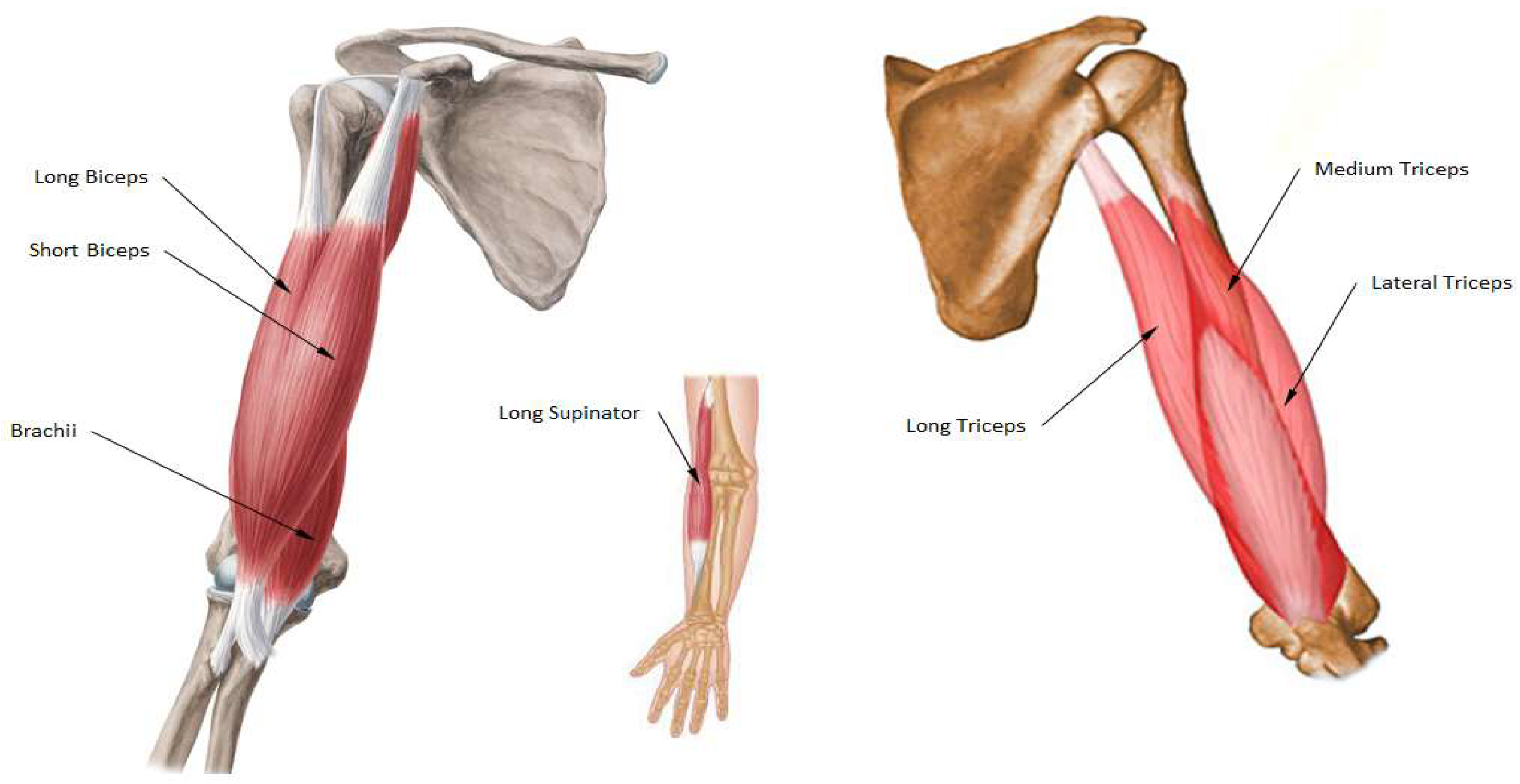
• Long biceps
• Short biceps
• Brachii
• Long supinator
• Long triceps
• Medium triceps
• Lateral triceps

Since muscles can only work under traction (they do not transmit compression loads), different models must be proposed for a separate study of the triceps and biceps muscles. Several analyses, on different aperture angles of the elbow, will be solved looking for the effort needed on referred muscles, biceps or triceps, to balance 150 N applied on the wrist in an “isometric contraction”. The scope of the study includes the following aspects:

• Analyzing the elbow under load at different angles;
• Obtaining efforts in different muscles involved in the joint for different positions;
• Defining mathematical models to predict efforts in muscles depending on:
  • Joint angle or muscle length;
  • Applied load on the wrist.

2. Materials and Methods

The proposed methodology will allow one to calculate elbow muscle effort. Furthermore, a post-processing of the results is proposed in order to obtain the formulation of efforts in the studied muscles when the load applied changes. These efforts are referred to isometric load cases. An isometric load involves muscle contraction against resistance in which the length of the muscle remains constant. The research can be divided into two main parts:

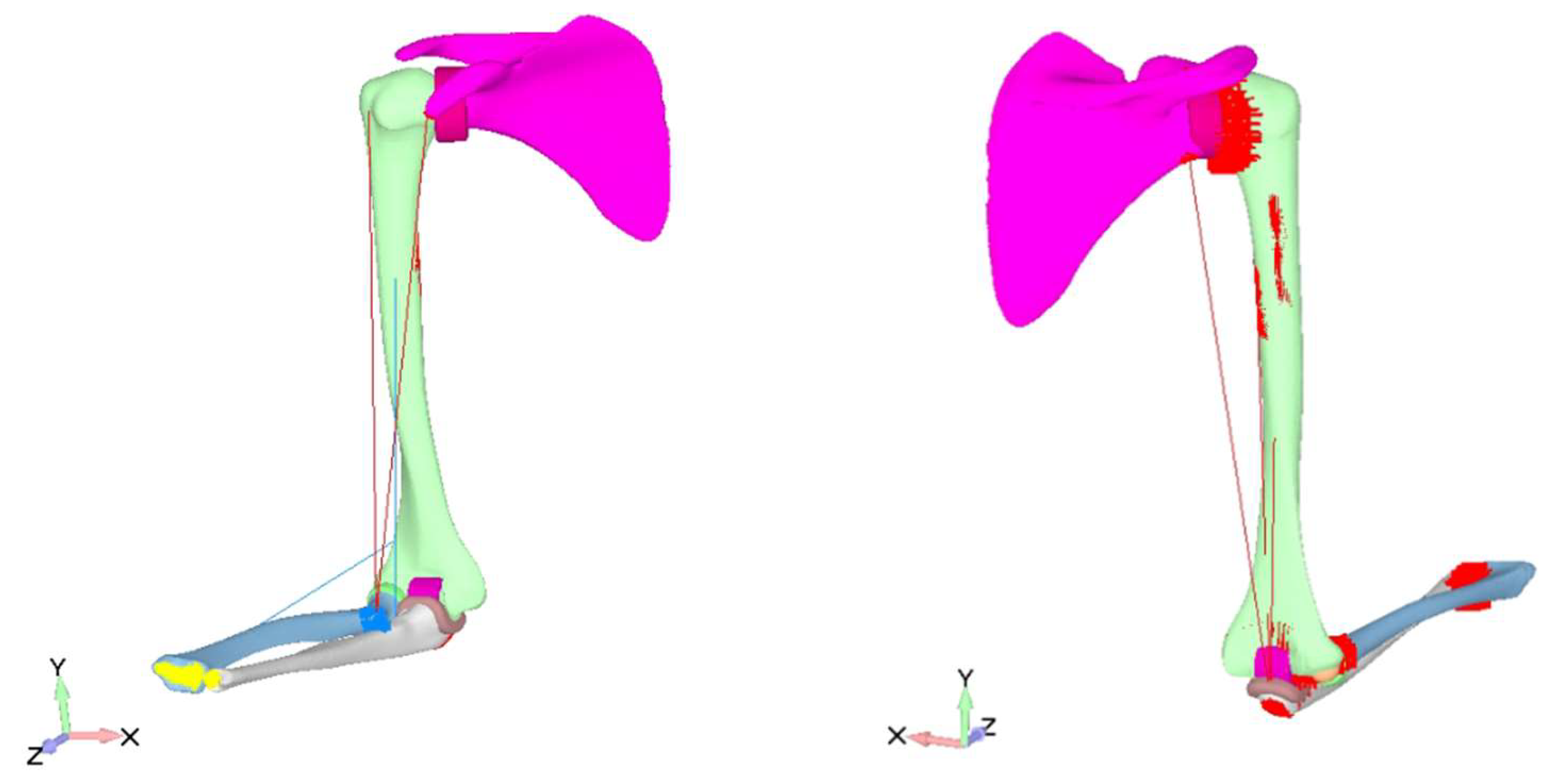
• Finite element models of the mechanism of elbow joint. The 3D anatomical model developed is based on two diagnostic imaging techniques. CT for the bones and MRI for the muscles. From this three-dimensional model, different FEM models were generated, for biceps and triceps muscles studies.
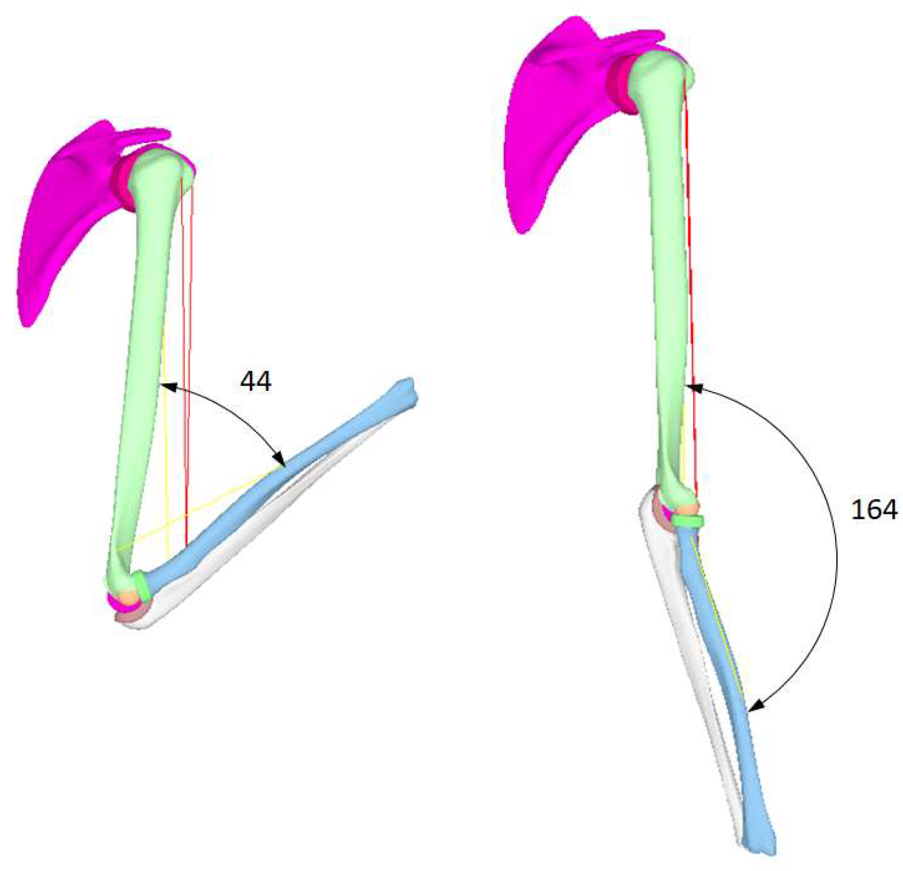
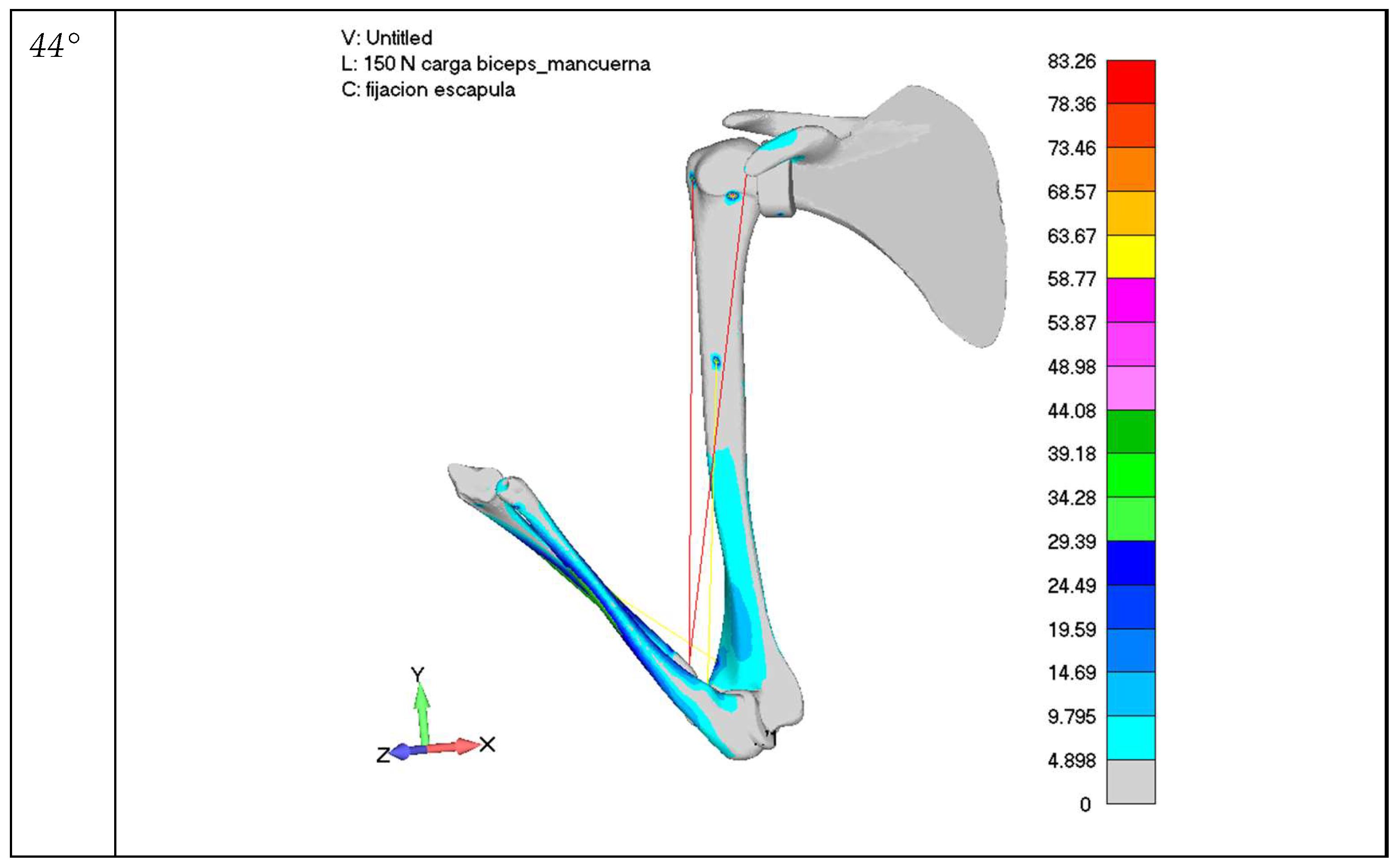
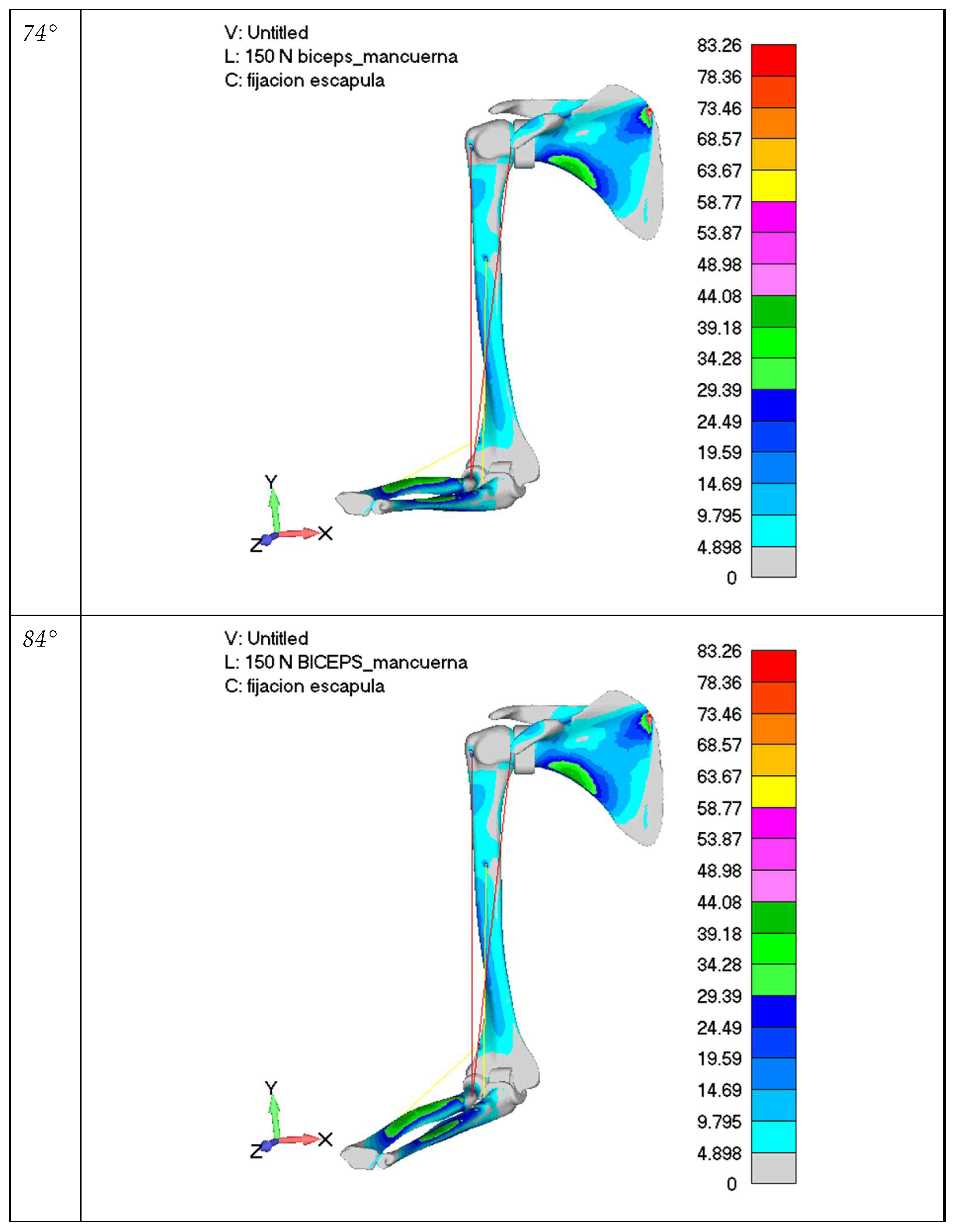
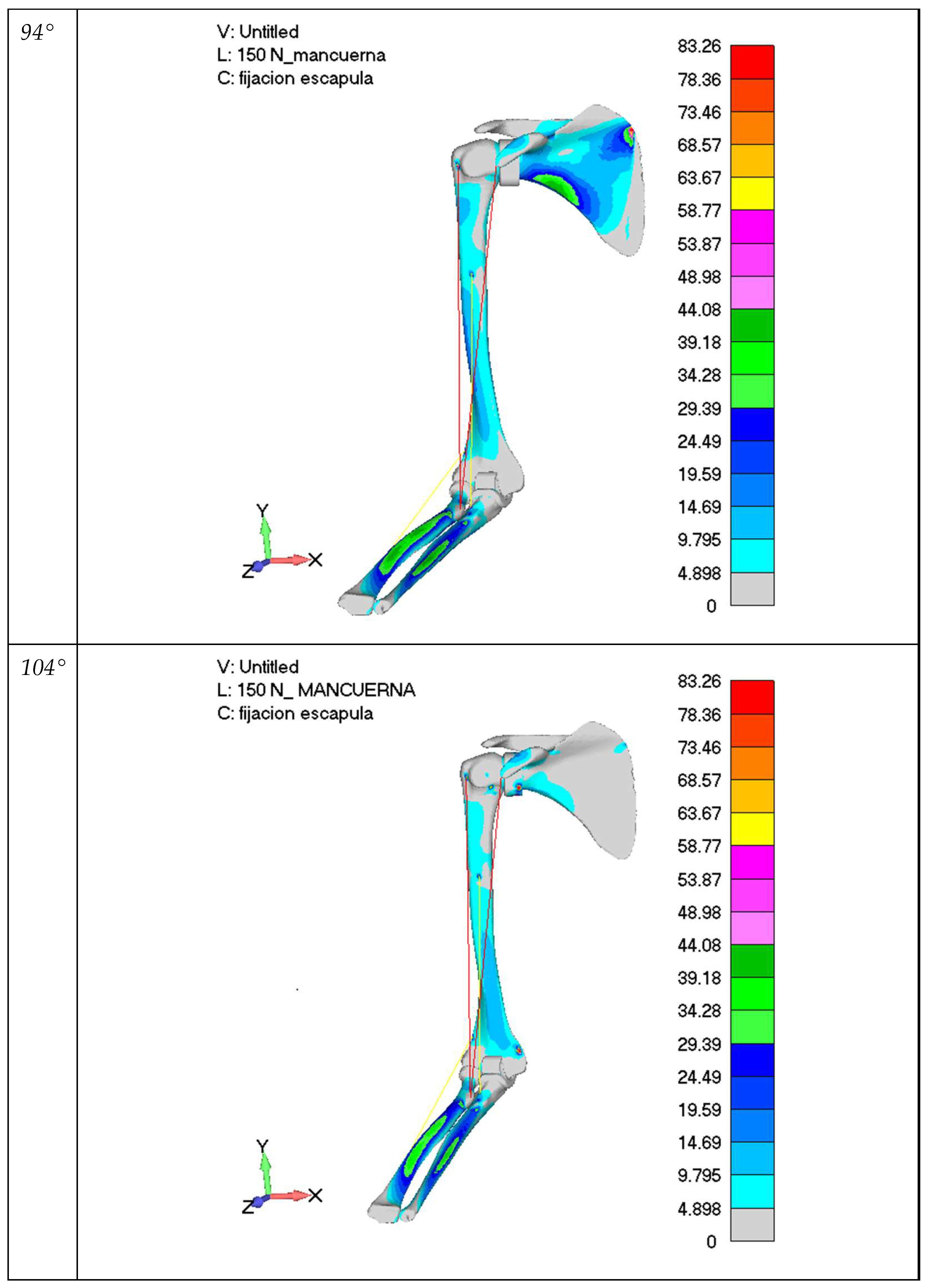
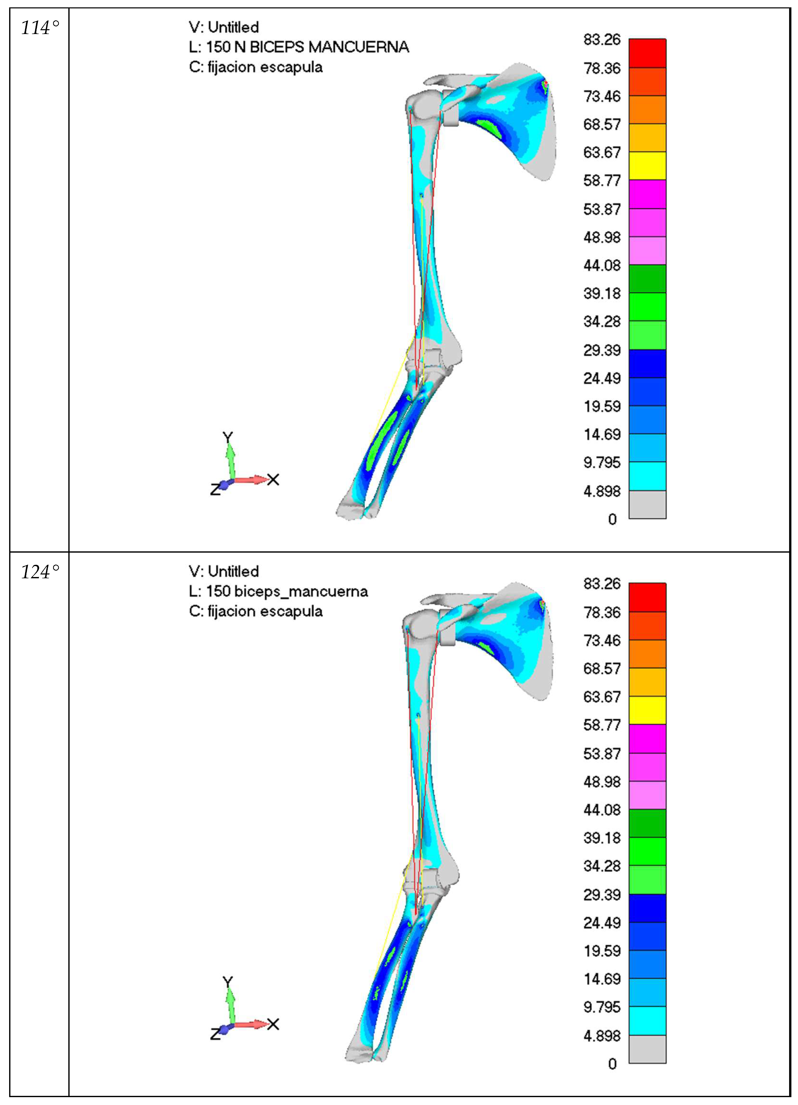
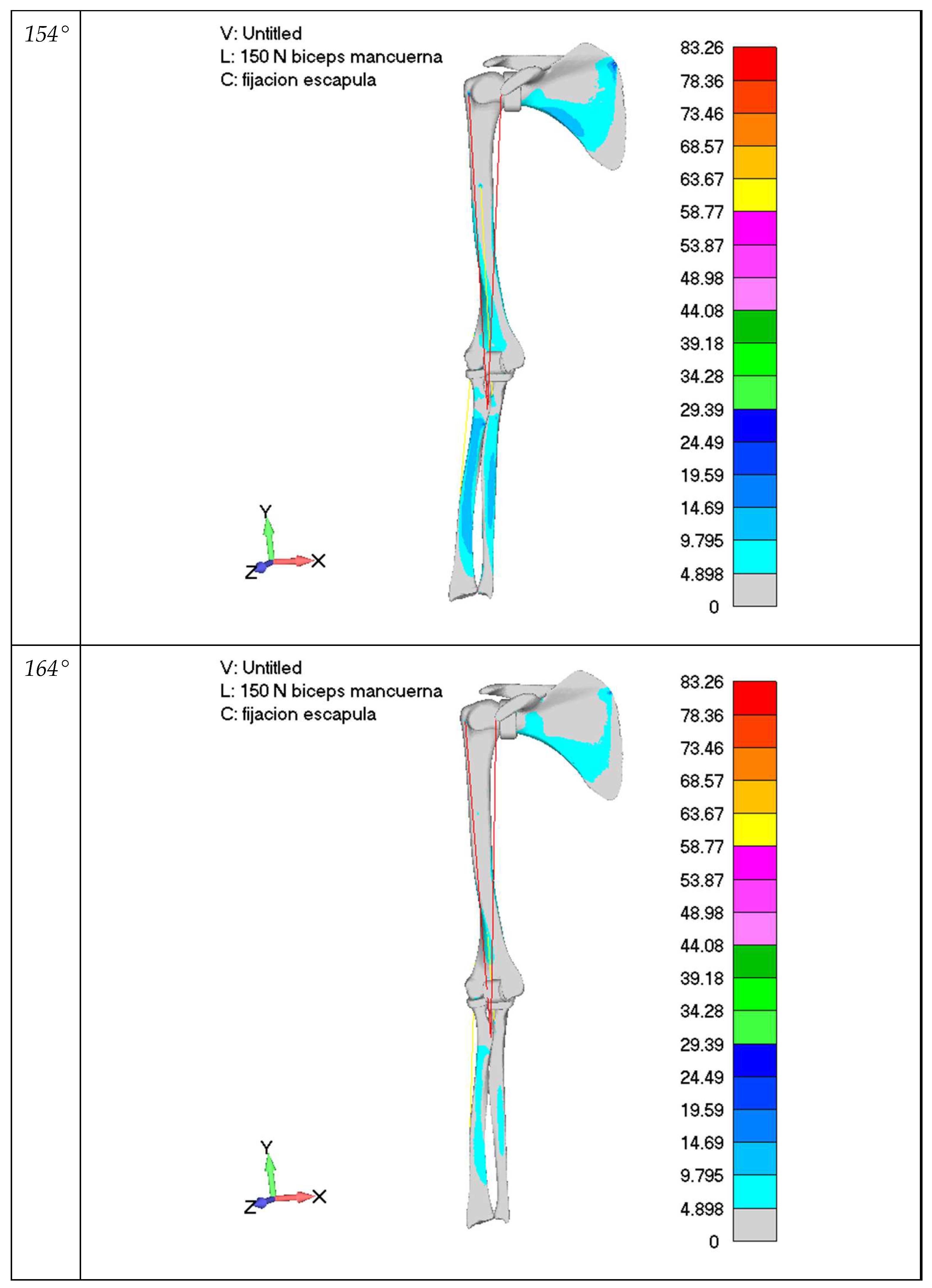
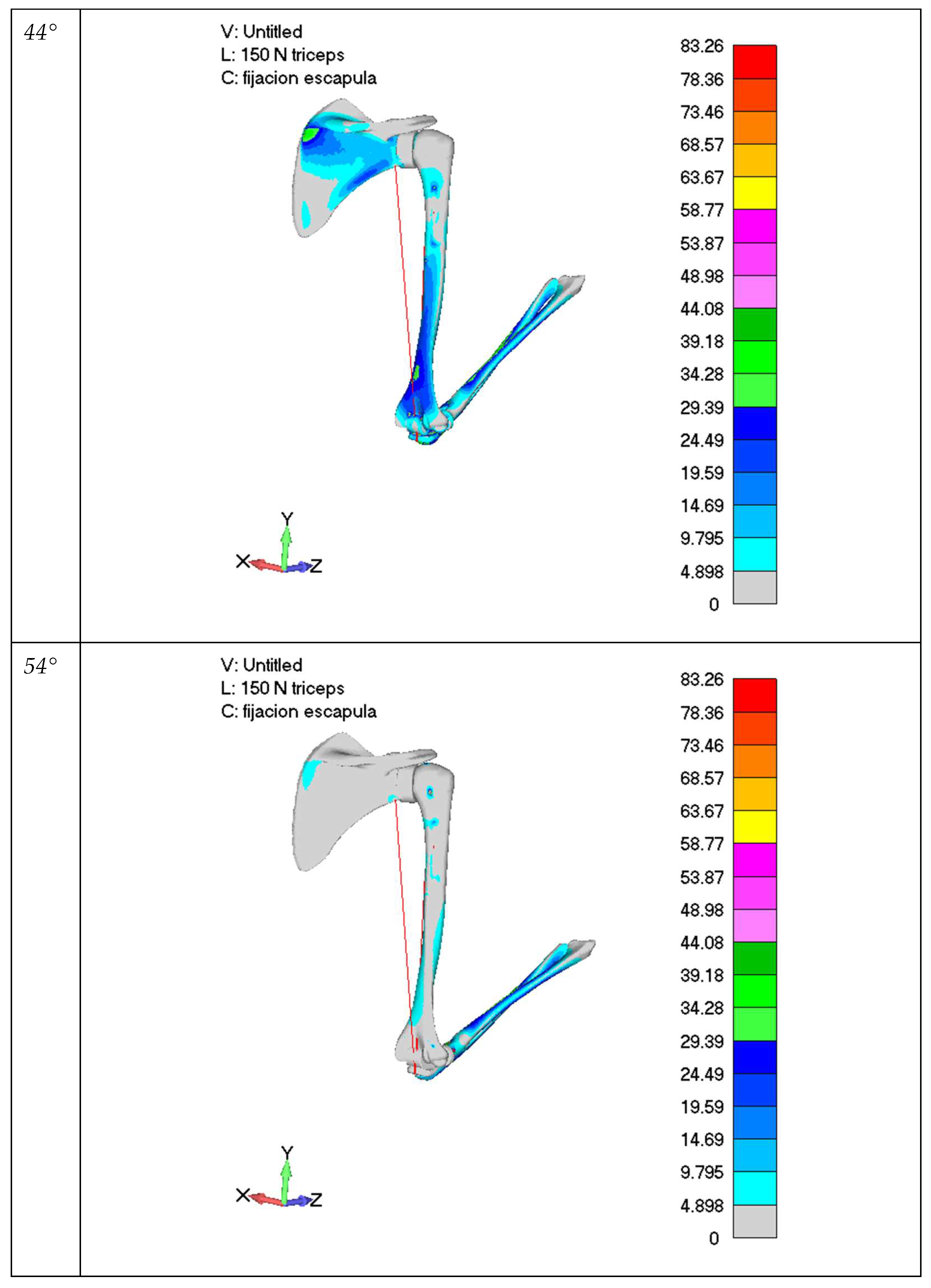
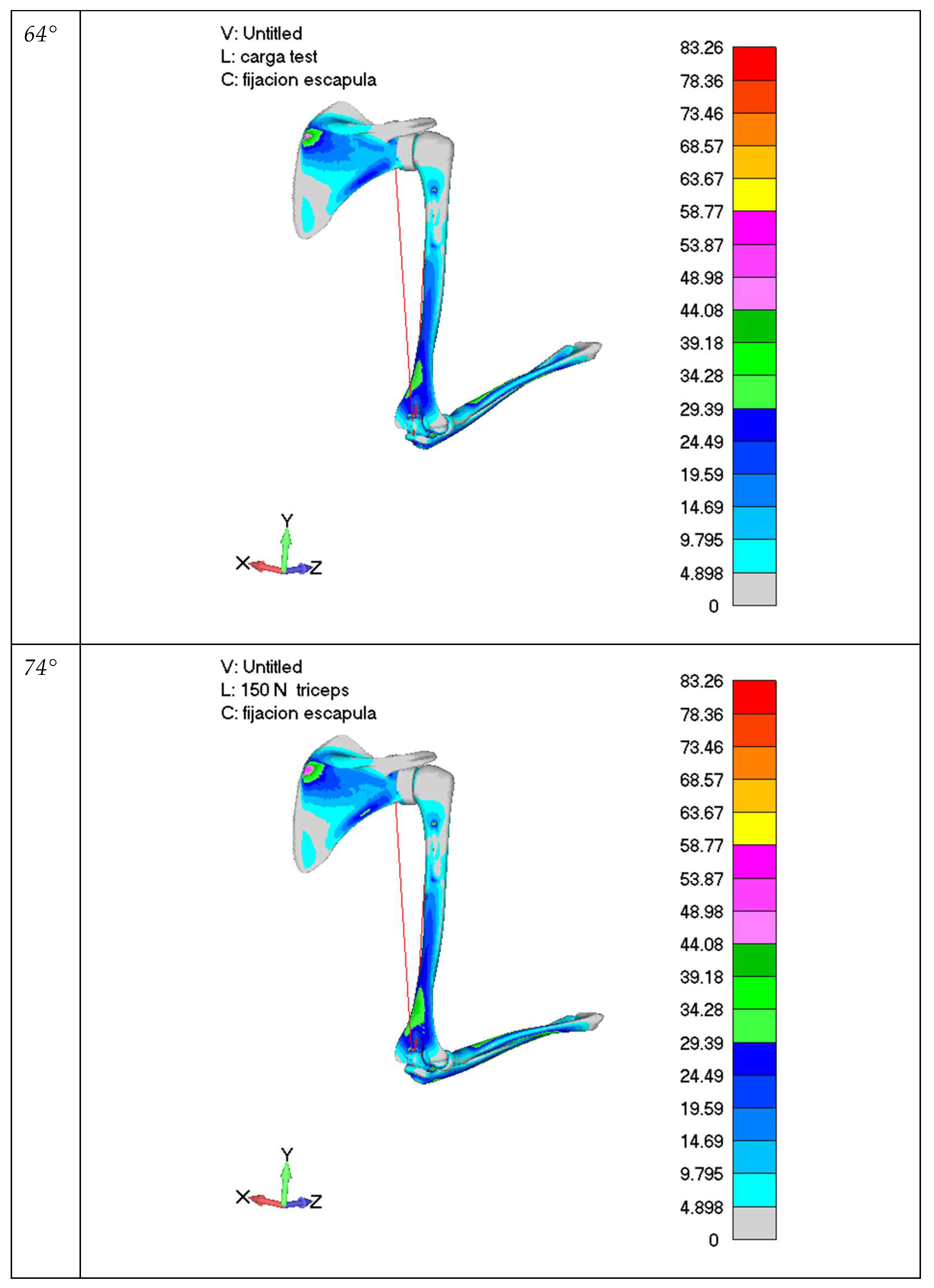
• Mathematical models predicting efforts in muscles studied. From FEM models, isometric muscle efforts will be obtained for a vertical load applied on wrist, 150 N including forearm mass, at different angles of aperture in the joint, from 44 to 164 degrees. These efforts will be extrapolated for any load applied on the wrist.

The first part is based on previous studies [25]. This model is shown in Figure 2, and it will be described in the more detail in next section.

2.1. Finite Element Model

For the creation of the FEM model, a 3D CAD model of the elbow joint is necessary, from which the mesh of the FEM model will be created.

Said CAD model is obtained starting from the images obtained by means of CT and MRI, of the elements of the joint (bones and muscles). Thanks to the use of software for generating 3D CAD models from point clouds, Geomagic Desing X, we can generate the CAD model of solid bodies.

The FEA model was implemented in Siemens FEMAP 10.2 as preprocessor and postprocessor, and NX Nastran 7.1, as solver. FEA software was described in detail in previous research [25]. Figure 3 shows the two developed FEA models for the biceps and triceps FEM analysis.

2.1.1. FEA Model Creation Meshing Process, Element Types

Different types of elements have been used for different components:

• Bones. They are meshed using 3D elements (tetrahedral type, 2nd order, 10 nodes). Teo et al. [26] use 3D elements for meshing neck and head parts of the joints in their study. In the same way, Donahue et al. [27] use 3D elements with axisymmetric condition, to model knee parts involved in the study.
• Cartilages. They are meshed using 3D elements (tetrahedral type, 2nd order, 10 nodes). Donahue et al. [27] and also Abidin et al. [28] model cartilages using 3D elements.
• Bone cartilage junction. Since the cartilage and bone form a solidary union between both parts, during the meshing process, a coincidence of the nodes of the bone and the cartilage in the contact area has been carried out. By ensuring that the bone and cartilage nodes coincide in that area, it is possible to ensure that the transmission of efforts between both parts is correct.
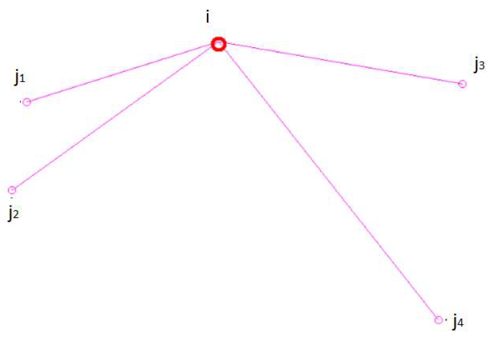
• Contact between cartilages. It has been modeled using rigid elements that join the nodes of both cartilage meshed parts involved in the joint, as explained in previous studies [25], using an RBE2 element. In the RBE2 elements used, the degrees of rotation freedom have been released so that only forces are transmitted in the X, Y or Z axes.
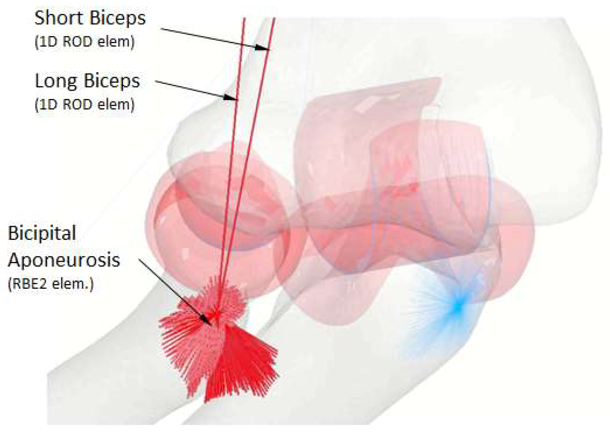
• Muscles. These are meshed using 1D elements (the type is discussed in this study). Previous studies have considered muscles in this manner, as 1D element acting along the imaginary axis of the muscle. Alonso et al. [20] model muscles in the leg to study human march in the same manner, 1D elements aligned with the axis of the muscles; Sachenkov et al. [29] use the same approximation for muscles, Parekh [30] approximates muscles to a 1D FEM element aligned with the muscle axis. This is a simplification, but it is used by several authors because fusiform muscles only have two insertion points and low pennation angles. Thus, fibers are aligned so with this imaginary axis which is formed by joining both insertion points.
• Tendons. These are meshed in combination with muscles, as a unique element musculotendon (MTU). The same 1D element is considered for tendons.
• Tendon insertion in bone. It has been modeled by adding a rigid element (RBE2), joining the end node of the 1D MTU element with several nodes in the bone, and thus distributing the reaction force in the area of the insertion of the tendons, as explained in previous research [25]. Of the restrictions that an element with these characteristics can apply, only the displacements in the X, Y or Z axes have been applied, freeing the turns around them. In this way, and since the MTU only transmits axial forces, we eliminate any possible bending moments that may affect the insertion of the tendon in the bone.

The RBE2 elements constitute constraint equations between the nodes to which the element is connected, they are characterized by having a node, called independent, and whose degrees of freedom are independent. The rest of the nodes connected to the RBE2 element are called dependent, and in them it must be fulfilled that the displacements of the independent node must be the same as in the dependent nodes.

That is why they are commonly known as rigid elements, since the distance between the component nodes remains unchanged.

In Figure 4, an example of an RBE2 element can be found, with an independent node (i) and four dependent nodes (j1 … j4).

The force balancing equation on an RBE2 is such that the reactions that appear on dependent nodes of the element must balance the force applied in the independent node:

$${\displaystyle \sum }_{dependent}\left\{Reactions forces\right\}=F_{independent}$$

(1)

In this way, using an element of this type to simulate tendon insertion in the bone, the stress that appears in the 1D element that simulates MTU in the insertion zone is distributed, eliminating stress concentrations.

Figure 5 shows the application of this insert model.

2.1.2. FEA Model Creation Muscles Modeling

Given that the proposed study is focused on knowing the forces developed by each of the muscles of the elbow joint, in different load situations, the modeling of the muscle must be such that it allows one to obtain these values.

As mentioned above, the objective is to be able to use a 1D element that allows us to reuse the mesh created to solve the FEM simulation without the need to re-mesh the entire model for each position of the joint.

The behavior of the element used in our study to simulate the muscle in the joint must be such that:

• It works only in traction.
• The force of the element used must be generated along the axis that joins the two nodes that define it; it must not have transverse forces.
• It must not present deformations or displacements that alter the isometric character of the contraction studied. Therefore, the deformations have to be low.
• The 1D-type elements existing in FEM analysis tools are described below, also indicating the reasons that lead us to discard them as valid for our purpose.
• Constant spring stiffness. In this case, the results are not valid, since a spring delivers the force along a curve according to the equation F = K·x, where K is its stiffness (N/mm) and x is its elongation (mm). The use of this element would mean that a muscle would deliver a single force value for a given length, which is not true. A muscle at a given length is capable of delivering a force between 0 and the maximum force that muscle fibers are capable of developing.
• Variable spring stiffness. For the same reason as before, although in this case the maximum force could adjust according to the length of the muscle, it does not serve the purpose of the proposed study. The muscle can deliver a force between 0 and the maximum force for a given length. In the case of using a spring element, there is also the drawback of not always being able to balance the joint and the present study would no longer be isometric.
• Beam element. With this element, it is possible to obtain the necessary force in the joint to balance it. Beam elements are characterized in that they present axial, shear, and bending forces, and the muscles only transmit axial tensile forces.
• Rod element. The use of this element meets the study requirements; it only transmits axial forces, and we can decide on a rigidity in it such that the joint does not present large displacements and therefore it is no longer considered an isometric contraction.

In search of the element that best reflects the behavior of the muscle within the joint, the ROD element, given that it only presents axial forces, is the one that best suits the needs of the proposed mathematical study. However, the said element can work under tension and/or compression, which would alter the results. That is why two different FEM models are generated for the study of the biceps or triceps muscles. One in which the triceps muscles are re-moved, and another in which the biceps muscles are removed. In this way, and considering the direction of the applied load, it can be ensured that the analyzed muscles work only under traction.

Several tests have been carried out to define the characteristics of the ROD element that will be used, maintaining the objective of minimizing its stiffness and keeping the element deformations at low values so as not to lose the isometric load condition in the analyzes.

For these reasons, the elements used in the FEA models are defined as:

▪

Rod element (1D element);

▪

Constant cross section: 100 mm²;

▪

Material parameters:

▪

Young modulus: 2000 MPa;

▪

Poisson coefficient: 0.43.

This type of element transmits only axial forces. Its constitutive equation is shown below.

$$\left[\begin{array}{c}F\\ M\end{array}\right]=\left[\begin{array}{cc}{K}_x& 0\\ 0& K_T\end{array}\right]·\left[\begin{array}{c}{\epsilon }_x\\ {\alpha }_x\end{array}\right]$$

(2)

where

• F is the axial force in the element;
• M is the moment along the axis of the element;
• K_x is the axial stiffness of the element;
• K_T is the rotational stiffness along the axis of the element;
• ε_x is the length variation of the element;
• α_x is the angle rotated along the element axis;

To ensure that no torsional stresses are produced in the element, it is sufficient to assign a value of $K_T=0$.

2.1.3. Material Properties

The meshing process of the 3D bodies that comprise the model, bones and cartilage, has been carried out automatically using the meshing tool that includes Femap. The geometric characteristics of the elements used are common to both bones and cartilage; they are:

• Second-order tetrahedral elements, 10 nodes;
• Nominal element size 1.5 mm.

The materials considered for each body have the following characteristics, taken from the CES Edu Pack [31].

The use of an isotropic and linear material for cartilage has previously been used in those cases in which the duration of the applied load is less than the time constant of the viscoelastic properties of cartilage, around 1500 s. In this case, given that it is considered an isometric contraction, in which there is no displacement in the joint and the application time is considered well below the 1500 s indicated, it is possible to consider it as isotropic, linear, and elastic with the properties indicated in

Table 1. Tissue properties for bones and cartilages.

	Young’s Modulus (Mpa)	Poisson	Density (kg/m3)
Bone	17,200	0.41	1790
Cartilage	8	0.49	1150

. Donahue et al. [27] considered isotropic, linear and elastic tissue for cartilages in the knee joint in their study of tibio-femoral contact in the human knee joint, based on the time required to apply the load compared to the time constant for viscoelastic properties of cartilages, for the same reason. Abidin et al. [28] consider cartilage as an isotropic, linear and elastic material in their study on a human knee joint model and verification.

The use of an isotropic material for bone modelling is known and has previously been used, Teo et al. [26], meshed head and spine using 3D elements with bone tissue as isotropic, linear, and elastic.

2.1.4. Mesh Resume

The summary of the FEM mesh is as follows:

• Number of elements: 548,139;
• Number of nodes: 821,755;
• Number of second-order tetrahedral elements: 546,035;
• Number of 1D ROD elements: 4 (for biceps analysis) 3 (for triceps analysis);
• Number of rigid elements RBE2: 2100.

A study of the quality of the mesh, based on the Jacobian value of the elements, shows us how good its quality is for our objective. Figure 6 shows the elements that are below the limit value of 0.6 (good quality for the considered analysis).

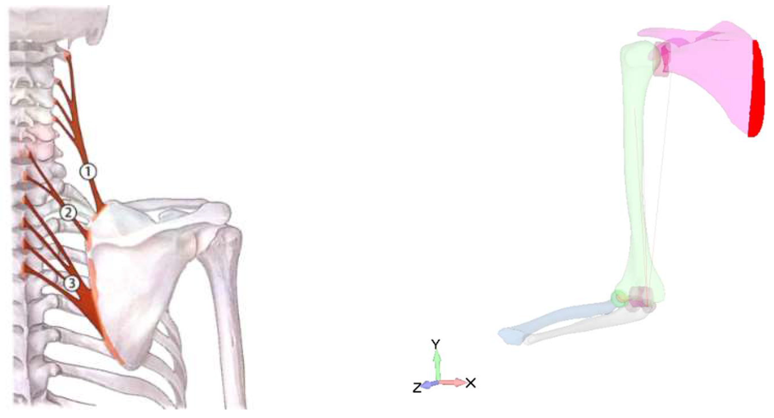
2.1.5. Boundary Conditions

For the boundary conditions, the scapula is considered fixed in the area (pink color on the below image) where the muscles of the scapula would be inserted. These muscles (see Figure 7) are:

• Levator scapula muscle;
• Rhomboid minor muscle;
• Rhomboid major muscle.

2.1.6. Load Application

In order to be able to validate results of the analysis, the load considered must be easy to replicate in a controlled environment; that is why we have defined the load as the mass of a dumbbell of 15 kg (approximately, 150 N) for the biceps analysis. In the case of triceps loading, the simulation is more similar to the exercise done using a guided load machine.

The application point of this load is the wrist (the hand is not modeled) and although this can affect slightly to the results, due to the difference in distance of the load applied in the joint, this can be solved varying the load as needed when applied in the hand.

All models have the same load applied, at the same node, and in the same vertical direction (see Figure 8).

The load is applied in vertical direction, positive axis (ascending) when analyzing the triceps and vertical direction, negative axis (descending) when analyzing the biceps. All load cases are considered as static load cases, isometric contraction of the muscle, and, to avoid compression loads on muscles, two different models have been developed; one of them includes only biceps muscles, with descending load, and the other one includes only triceps muscles, with ascending load.

In the model, gravity force has also been considered. Thus, the mass of the arm is considered in the analysis.

To do so, the density of elements has been modified so that the values of the upper arm and forearm mass are [32]:

• Forearm mass: 2.5 kg;
• Upper arm mass: 4.3 kg.

All load cases are considered as static load cases; due to the isometric contraction of the muscle, there must be no displacement in the joint.

2.1.7. Design of Experiment

The FEM model is considered linear and static. No non-linearity has been considered, neither in the materials nor in the restrictions of the model. That is why the general equation of the calculation is so important and can be written as follows:

$$\left[R\right]=\left[K\right]·\left[U\right]$$

(3)

where

[R] = global loading matrix;

[K] = global stiffness matrix;

[U] = global displacement matrix.

Equation (3) can be solved directly using the Gauss elimination method, there is no iterative process, and the solution is unique.

The resolution of the problem is carried out through several linear static analyses, each one of them representing a different load condition in the joint, and the result of them is the necessary effort in each muscle of the joint to balance the applied force on the wrist.

As mentioned above, there are two different models, thus guaranteeing that the muscles work only in traction, to study the biceps and the triceps muscles.

In each of the models, the configuration of the joint will be modified by varying its angle between 44 and 164°, at intervals of 10°.

The applied load will always be 150 N.

As a reference for the reading of the results, the fully extended arm corresponds to 164 degrees and the fully flexed arm corresponds to 44 degrees (see Figure 9).

2.1.8. FEA model Solution

The FEA model has been solved on a workstation with the following characteristics.

• Windows 10, 64-bit, operating system;
• Intel(R) Core (TM) i9-10900X CPU @ 3.70 GHz Processor (20 cores);
• 128 GB RAM memory;
• 1 TB SSD disk drive.

The solution time for any configuration is approximately 20 min.

As contacts in cartilages have been replaced by rigid elements, RBE2 type with free rotation on both nodes, the solution time has been reduced from 67 h to 20 min.

As described in a previous study [23] the results, comparing the model with contacts and the model with rigid elements instead, are similar in both cases, and therefore the use of rigid elements improves the efficiency of the analysis.

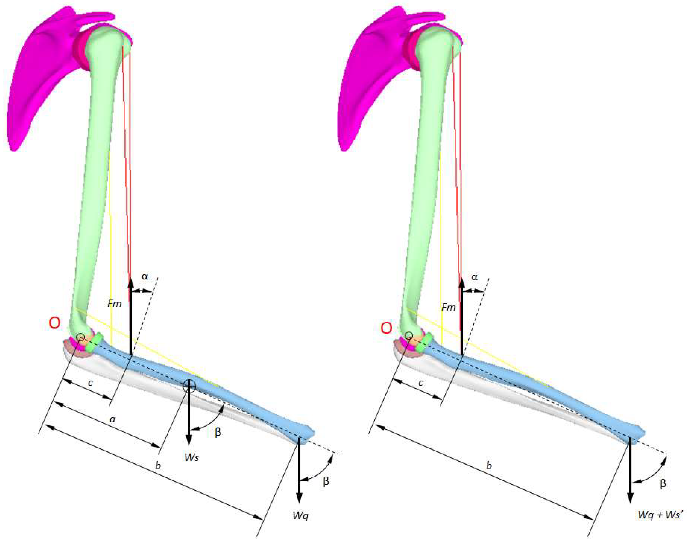
2.2. Mathematical Approach

In this work, several mathematical models are derived from the results of the FEM simulation. First, there are grade 6 polynomial curves, which represents the efforts of the five muscles involved for the simulated cases, described in previous section, for a vertical force of 150 N applied on wrist. Muscle effort is defined as the total force that appeared in the 1D element used for each muscle in FEM models. These models make it possible to obtain this effort for each muscle by following an equation for each muscle, with the following general formulation:

$$Muscl{e}_{effort}={\displaystyle \sum }_{i=0}^{i=6}{a}_i·{\alpha }^i$$

(4)

Once the forces needed in muscles have been calculated to balance the joint, with different angles and with a load of 150 N applied at the wrist, a mathematical approach will be proposed for obtaining these efforts for other loads, due to the mechanism type considered in the elbow joint, the applied forces and torque analysis done in the joint. The value of the force exponent is 1 in all cases, so there is a linear relation between the force applied and the muscle reaction force [33]. According to this, the greater the force applied to the wrist is, the greater the muscle force must be, and both values are proportional. Figure 10 and the following equations justify this simplification in the analysis, where:

• $W_s$ means the weight of the forearm;
• ${W_s}^{\prime }$ means the equivalent force for W_s applied at the wrist. The moment created by W_s or W_s′ is the same referred to O point;
• $W_q$ means the load applied in the wrist;
• α means the angle between biceps axis and the normal to the radius longitudinal axis;
• β means the angle between the vertical and the longitudinal axis of the radius;
• a, b and c are geometrical dimensions.

The left image considers the proper mass of the arm located in its center of gravity. Balancing equation on that forces scheme, referred to O point scheme, is:

$$Fm=\frac{\left(W_s·a+W_q·b\right)·\sin \beta }{c·\cos \alpha }$$

(5)

Instead of using W_s, we can use W_s′, applied on the wrist (right image). This W_s′ should comply:

$$W_s·a·sin \beta ={W_s}^{\prime }·b·sin \beta$$

(6)

So, the balancing equation would be the following:

$$F_m=\left(W_q+{W_s}^{\prime }\right)\frac{b·sin \beta }{c·cos \alpha }$$

(7)

As seen in Equation (7), the relation between F_m and W_q + W_s′ is linear, and constant for a certain angle only depending on b and c and α and β angles.

According to this, the forces in the muscles when the load is different from the 150 N applied in this study (including the ${W_s}^{\prime }$ in this 150 N) can be obtained by the relation between the external load applied and the reaction in the muscle.

$$\frac{W_q+{W_s}^{\prime }}{F_m}=\frac{F_{ext}}{R_{musc}}=\frac{c·cos\alpha }{b·sin\beta }=constant\left(\alpha ,\beta \right)=\frac{150\mathrm{N}}{F_m\left(150\mathrm{N}\right)}$$

(8)

In summarizing, forces in muscles depend on:

• Muscle length (or elbow angle);
• Force applied to wrist.

By applying these mathematical approaches, several polynomial equations have been obtained, one per muscle, which establishes the relation between force in muscle as:

$$F_m=F_m\left(W,\alpha \right)$$

(9)

where:

• $F_m$ is the force in the muscle (N);
• α is the angle of the elbow;
• $W=W_q+{W_s}^{\prime }$, is the load applied on the wrist (N).

In all mathematical models of muscle efforts, the effort could be obtained for any angle, $\alpha$, and for any vertical load, $f_v$. If the forearm mass, $m_{fa}$, is considered and $g$ is the gravity acceleration (9.81 m/s²) ${W_s}^{\prime }$ can be expressed as follows:

$${W_s}^{\prime }=W_s·\frac{a}{b}=m_{fa}·\left(\frac{a}{b}·g\right)$$

(10)

Thus, for obtaining the effort:

$$Effort\left(f_v\right)=F_m\left(f_v+m_{fa}·\left(\frac{a}{b}·g\right),\alpha \right)$$

(11)

General equations will be obtained describing the effort in each muscle depending on the angle of the joint and the load applied. These equations and their surface representations will be the results of this research. Both of them, the equations and surfaces, have been obtained using the curve fitting tool from MATLAB. It has been noted that these effort models for the five involve muscles are only used to study isometric muscular contractions, when muscle length does not vary.

3. Results

The model analyzed includes all muscles in the elbow joint, but the post-processing results are only applied to the biceps and triceps muscles.

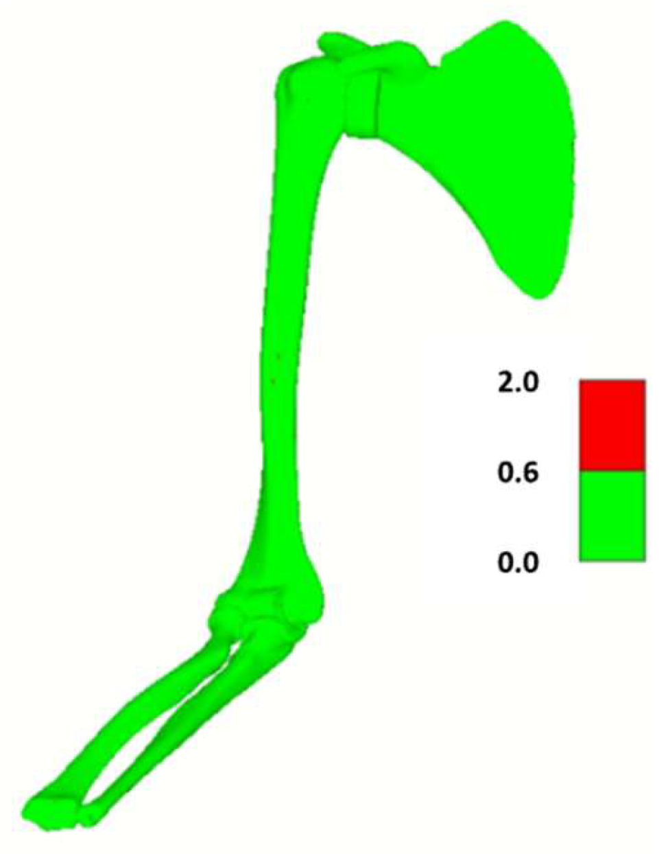
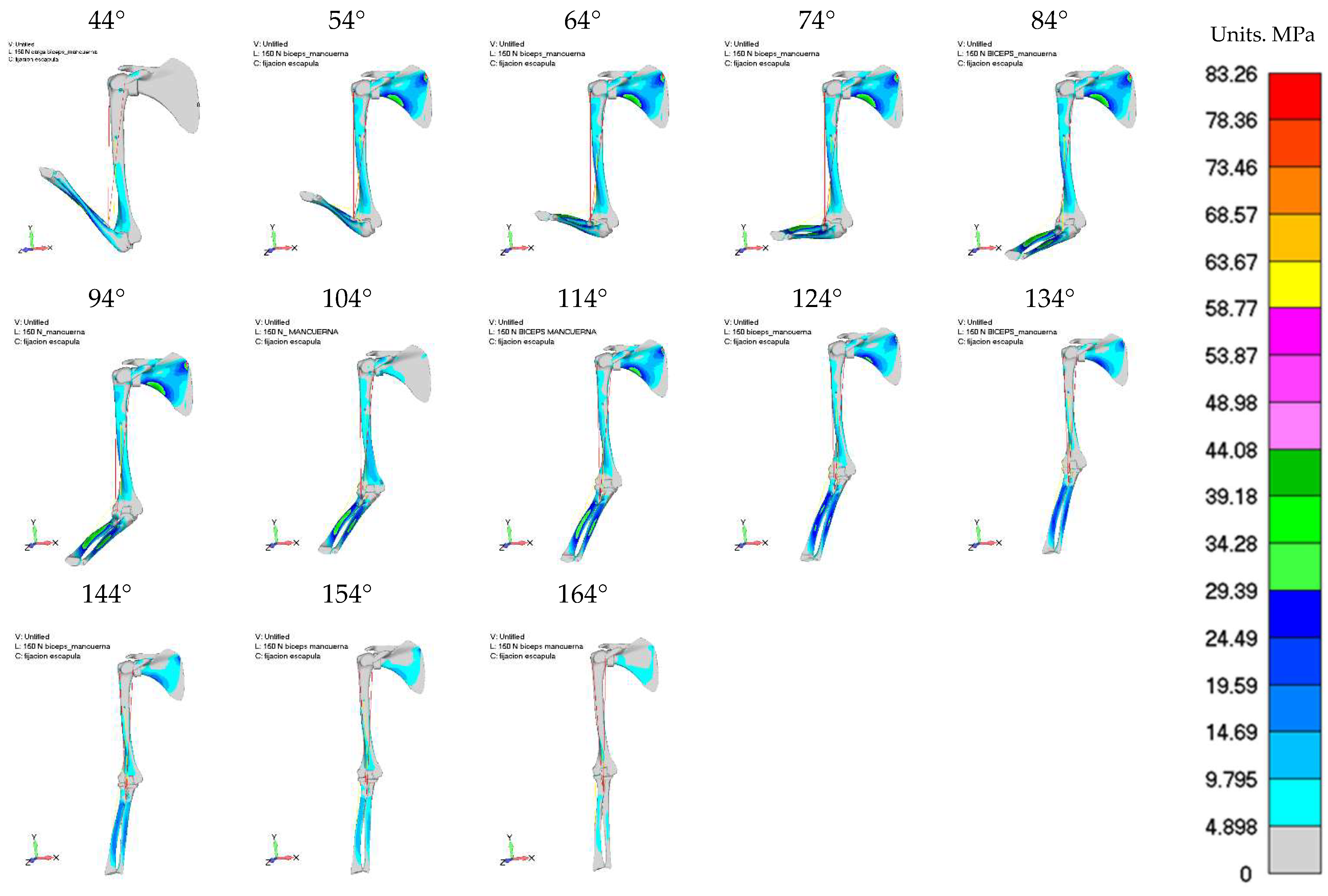
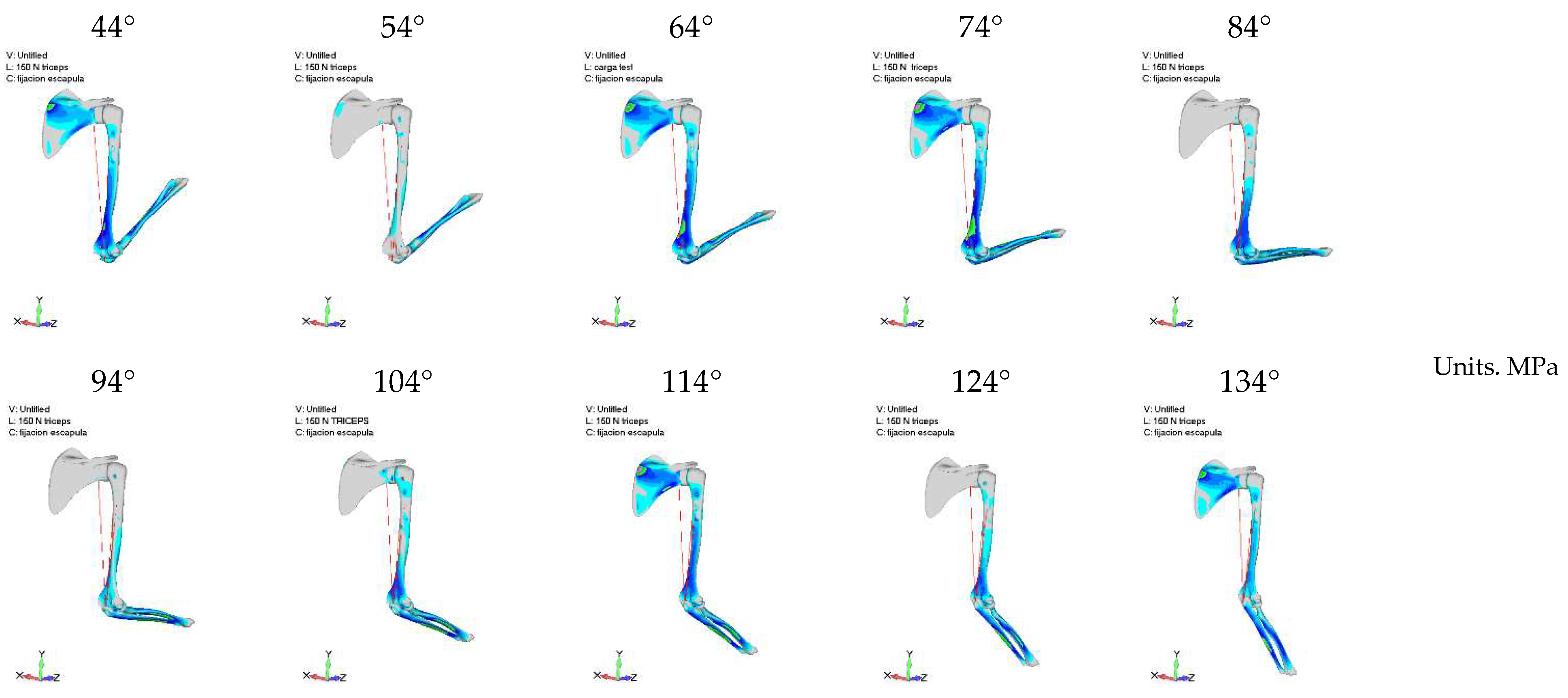
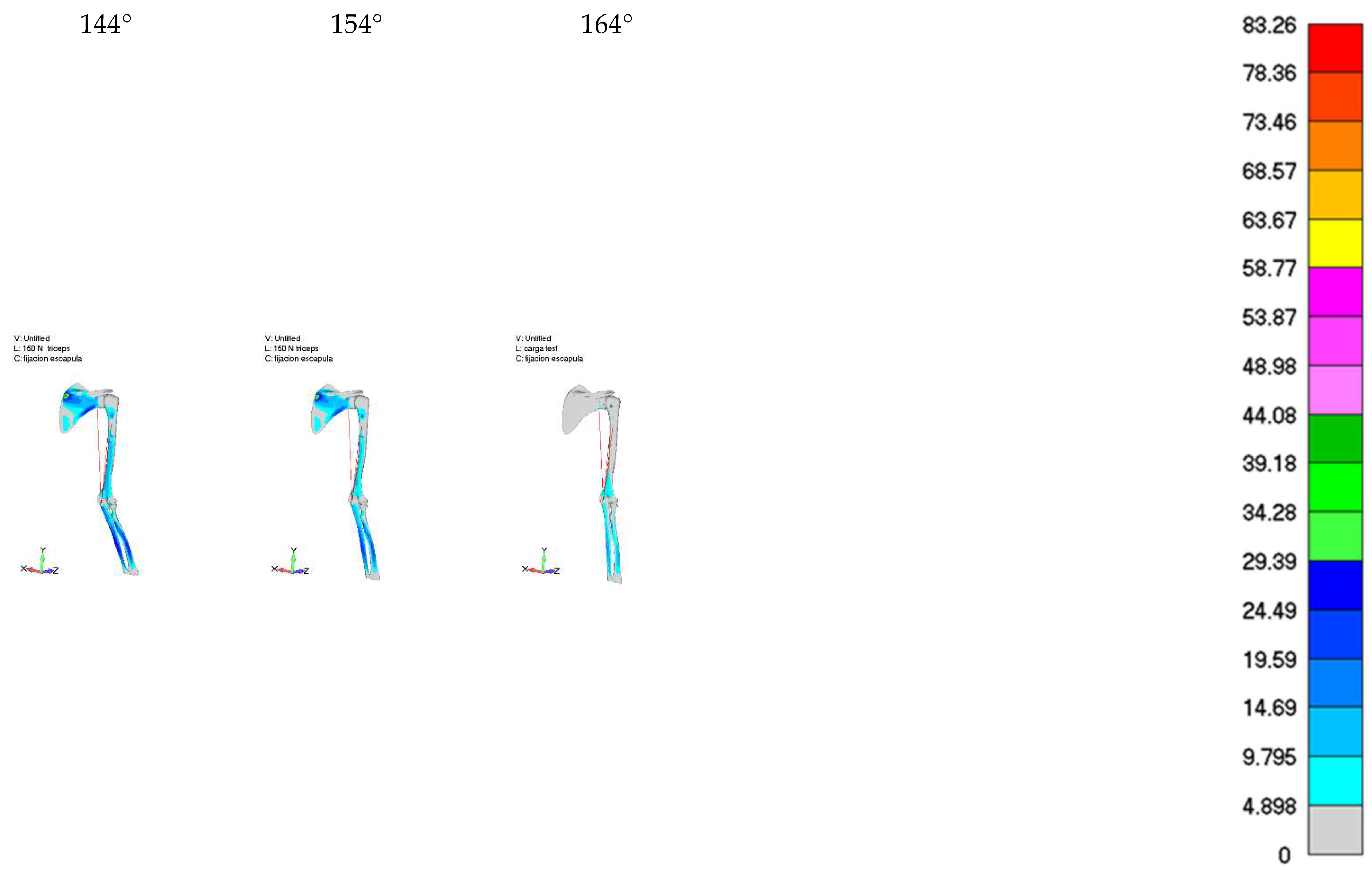
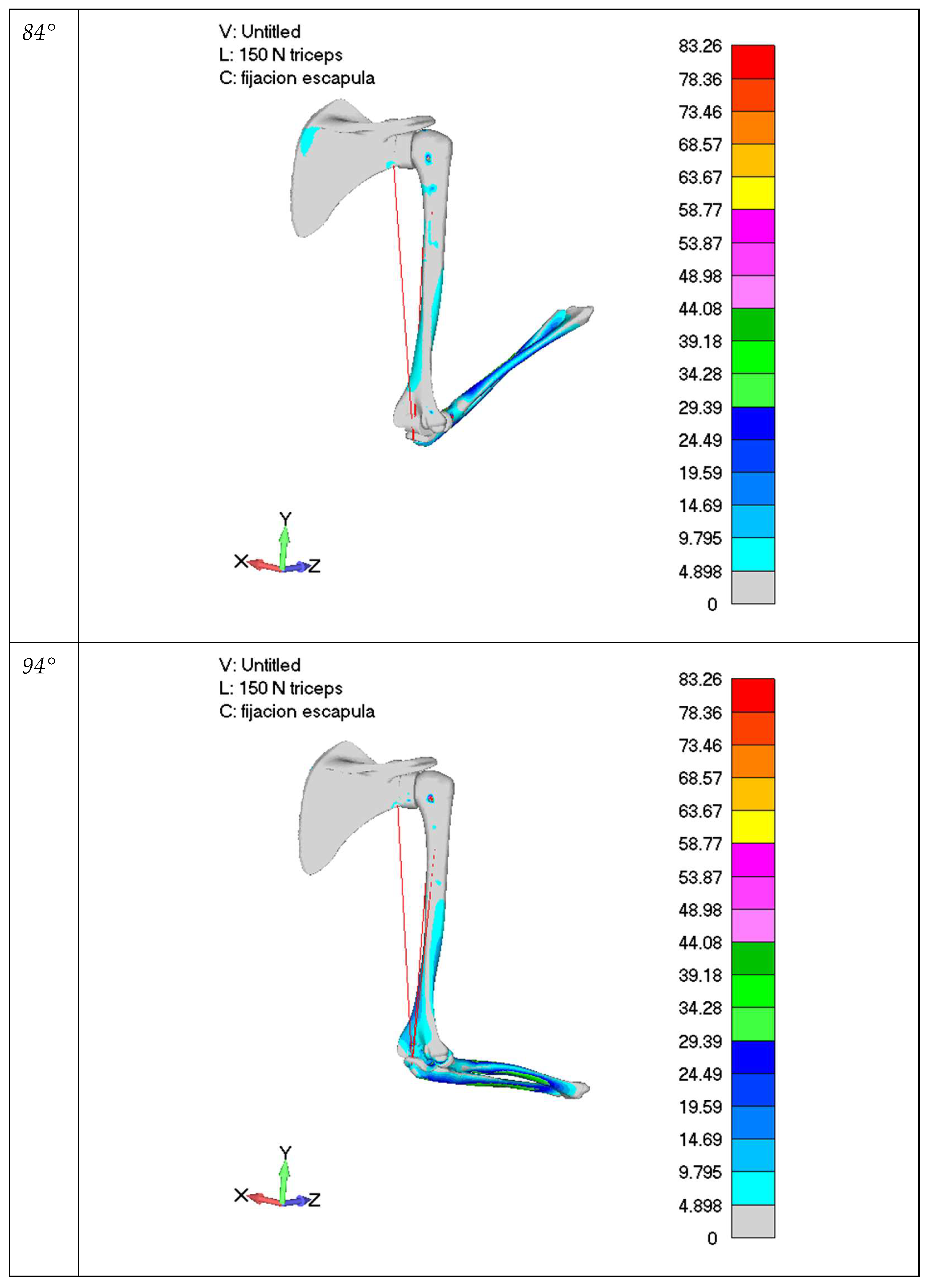
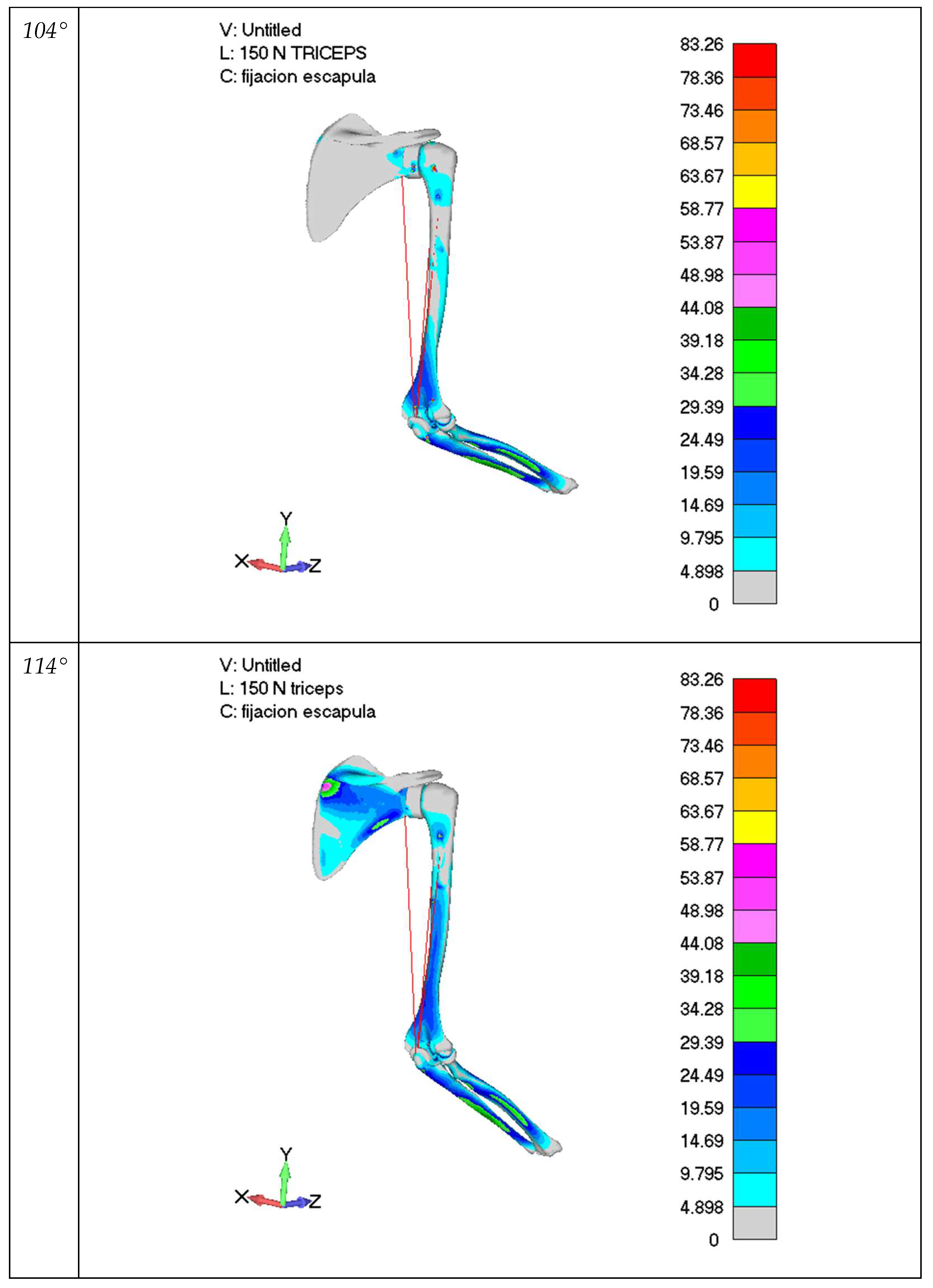
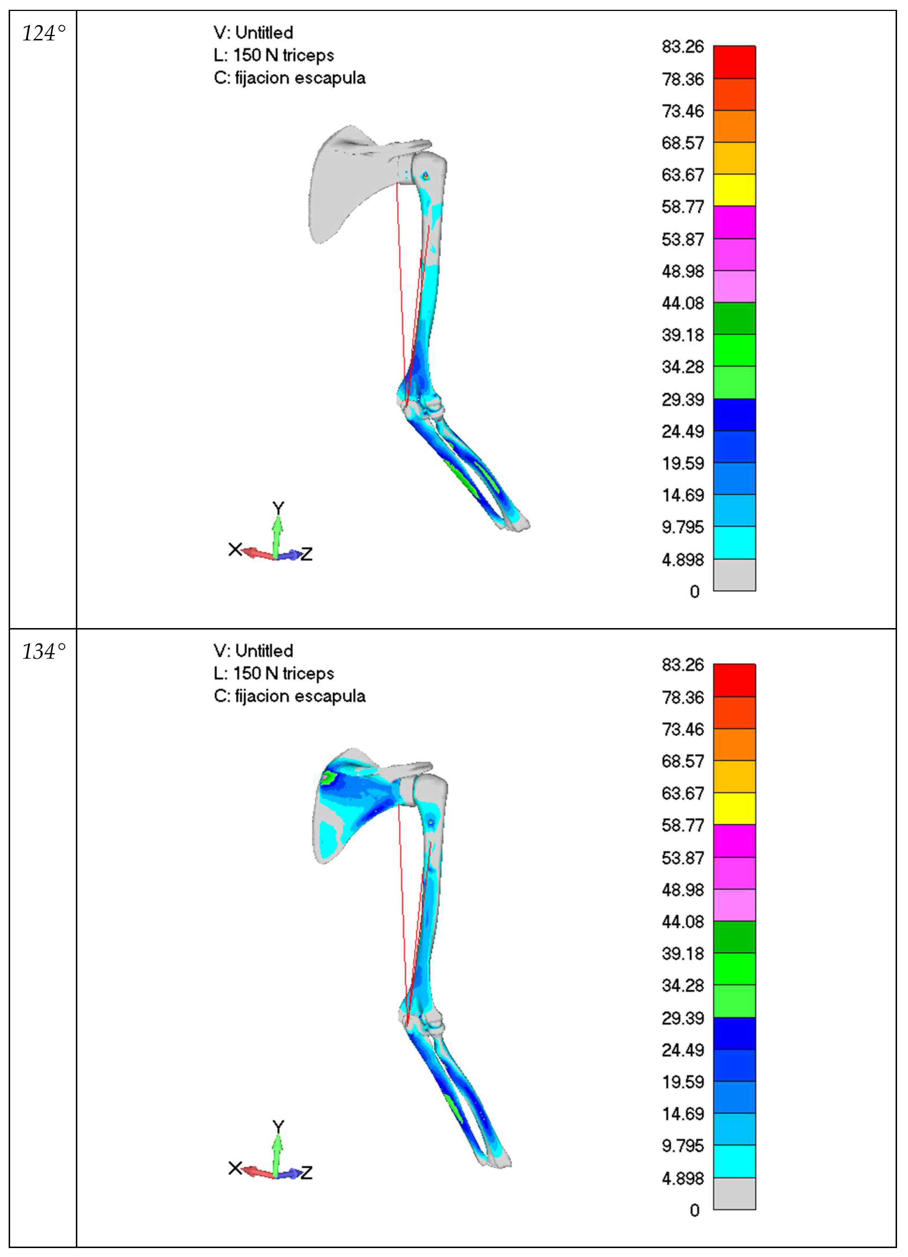
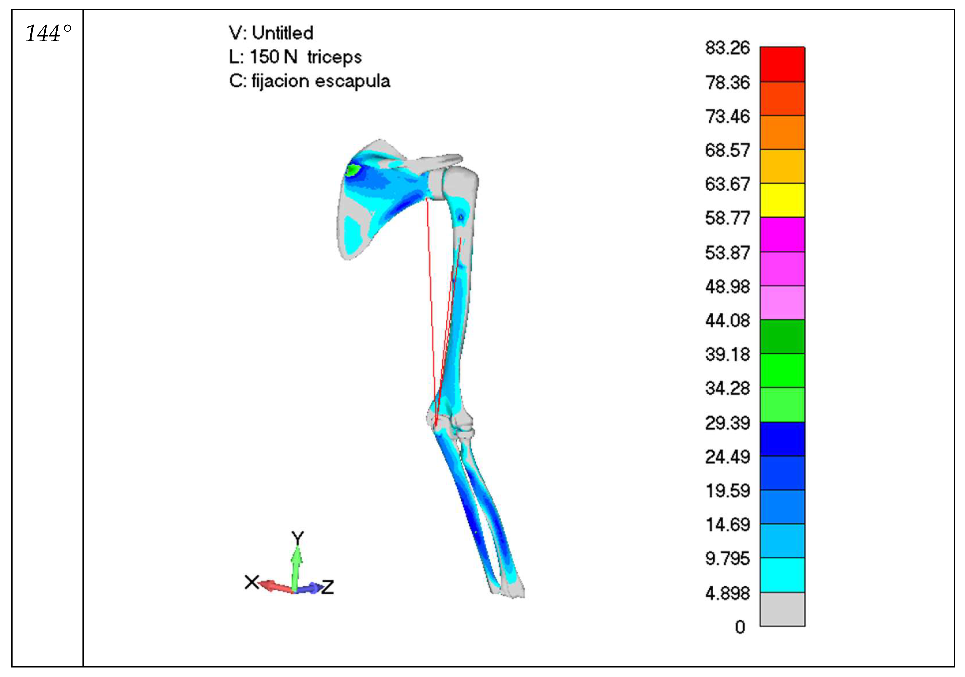
3.1. FEM Simulations, 3D Results

Figure 11 shows the results of running the design of the experiment described hereinbefore for the 13 cases of elbow angle for the biceps model. The figure represents the Von Mises stress in the involved bones due to the action of the 150 N as a vertical force (descendent) on the wrist. Each of the images represents the stress map resulting from the study of an isometric contraction in the elbow joint at the angle indicated in the image for a load of 150 N applied to the wrist, vertically and downward.

Similarly, Figure 12 shows the Von Mises stresses on the bones due to the FEM simulation of 150 N of vertical load (ascendant) on the wrist. Each of the images represents the stress map resulting from the study of an isometric contraction in the elbow joint at the angle indicated in the image for a load of 150 N applied to the wrist, vertically and upward.

3.2. Numerical Axial Efforts on Main Different Muscles

This subsection collects axial efforts on biceps and triceps involved muscles for the 26 FEM simulations (13 for biceps and 13 for triceps). These efforts correspond to the reaction obtained in the muscle itself, and length corresponds to the length of the muscle (the whole muscle length including tendons) measured in the FEA model, in that certain elbow angle.

Table 2. Axial efforts (N) in main simulated muscles, 150 N applied on wrist. Isometric contractions at each angle value considered.

	Long Biceps		Short Biceps		Lateral Triceps		Medial Triceps		Long Triceps
Elbow Angle (°)	Force (N)	Length (mm)	Force (N)	Length (mm)	Force (N)	Length (mm)	Force (N)	Length (mm)	Force (N)	Length (mm)
44	244	373	96	310	148	217	70	211	269	284
54	330	375	136	312	128	216	144	209	312	282
64	341	383	152	320	212	215	115	208	340	281
74	341	391	161	328	208	215	119	208	347	281
84	340	399	168	336	235	214	150	207	340	280
94	333	407	170	344	263	214	186	207	347	279
104	302	415	181	351	233	213	164	207	331	279
114	301	422	159	359	233	213	176	206	307	278
124	274	429	143	365	213	211	170	204	271	276
134	261	435	95	371	177	207	150	201	226	273
144	185	439	87	375	131	203	120	197	175	269
154	121	442	46	379	79	199	82	192	119	264
164	52	445	1	381	24	194	40	188	58	260

has these results if the form of force and the corresponding length for this applying force for all muscles studied:

• Biceps muscles (long and short biceps);
• Triceps muscles (lateral, medial and long triceps).

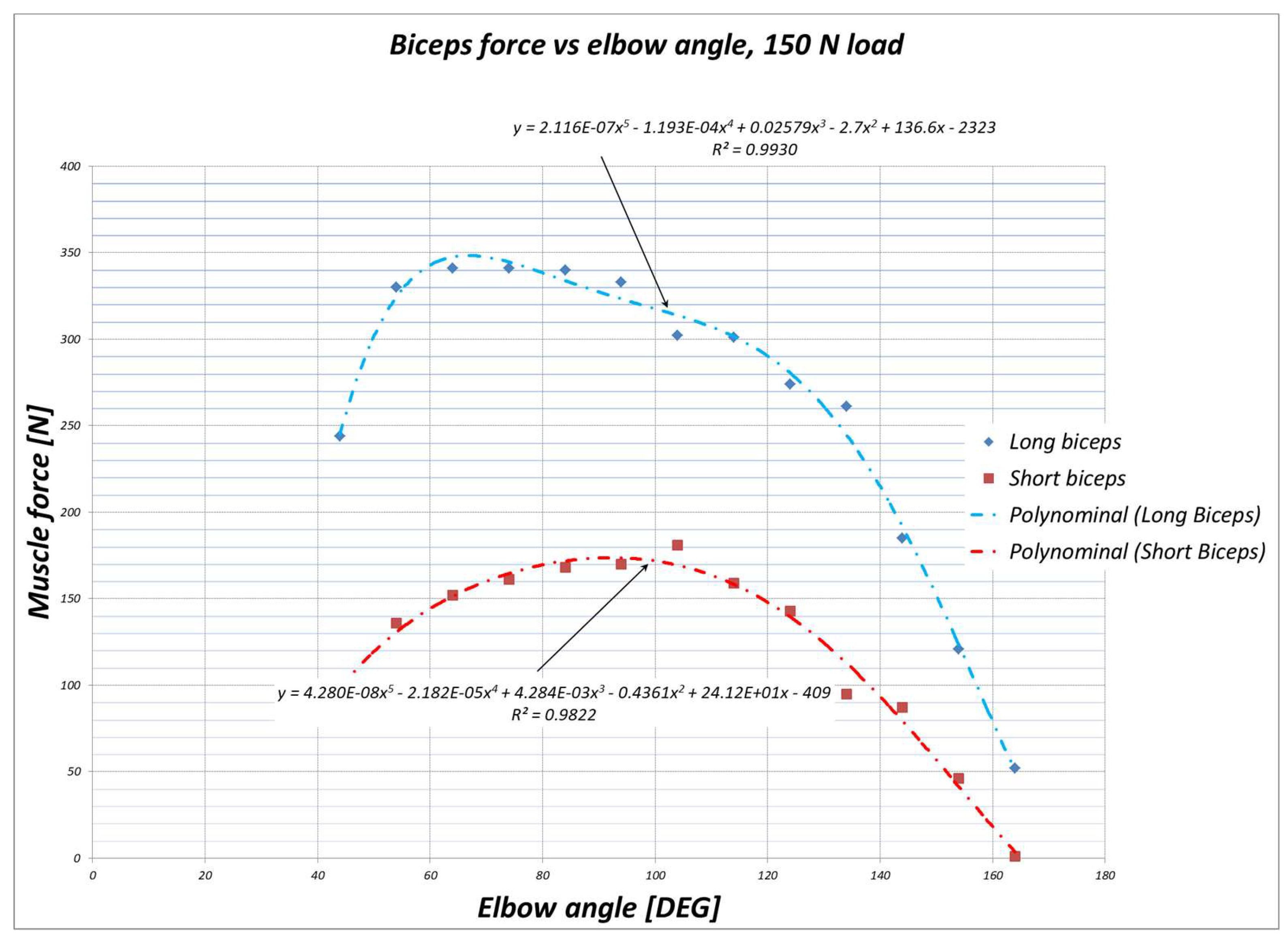
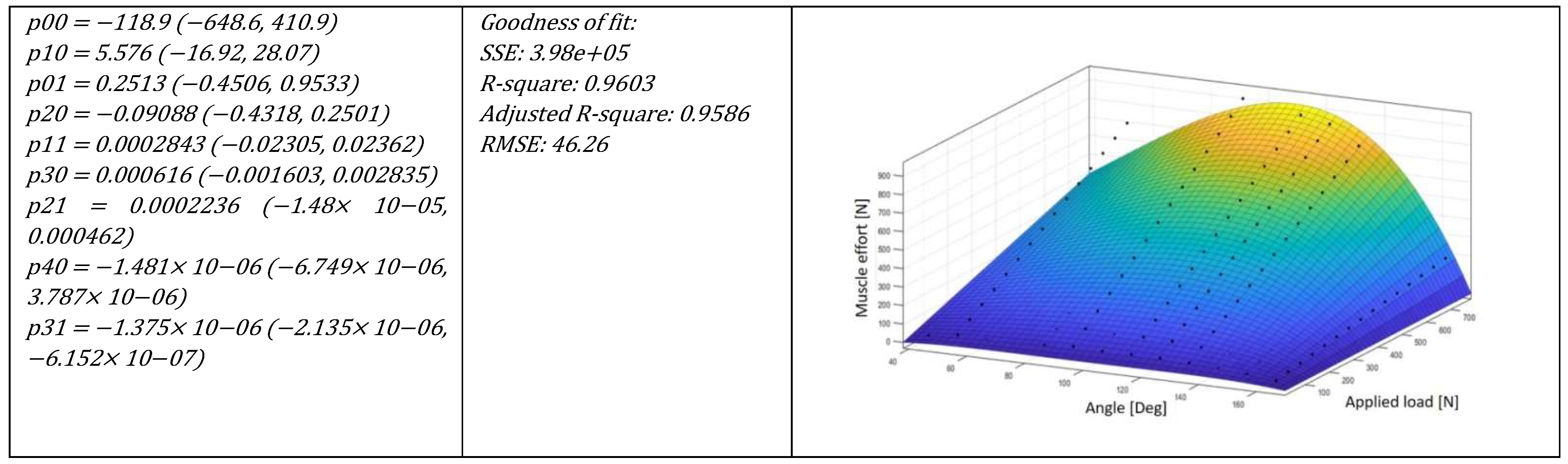
3.3. Mathematical Models for Muscle Efforts

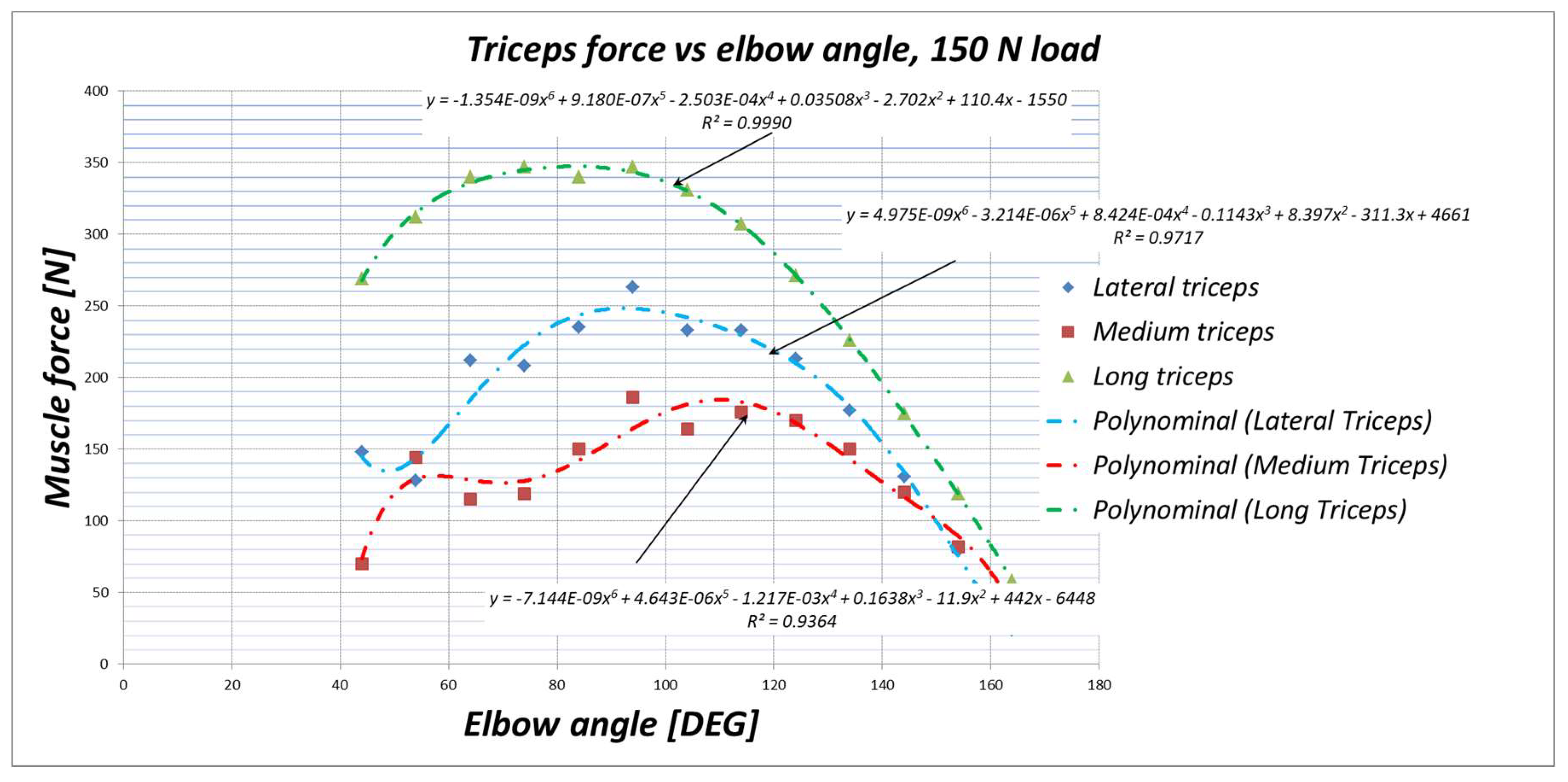
3.3.1. Efforts for 150 N of Vertical Load

The obtained R-square values are 99.3%, 98.2%, 99.9%, 93.6%, and 97.2%, respectively (see

Table 3. The equations developed as polynomial curves of grade 6th, based on the general formulation of Equation (4), has the following constant values for each muscle involved.

Muscle	a0	a1	a2	a3	a4	a5	a6	SSE	R2	RMSE
Long biceps	−2323 (−3730, −916.1)	136.6 (55.39, 217.8)	−2.7 (−4.477, −0.9232)	0.02579 (0.007278, 0.04431)	−0.0001193 (−0.0002116, −2.692 × 10−5)	2.116 × 10−7 (3.433 × 10−8, 3.889 × 10−7)	0	694.5	0.993	10.76
Short biceps	−409 (−1729, 911.5)	24.12 (−52.09, 100.3)	−0.4361 (−2.104, 1.232)	0.004284 (−0.01309, 0.02166)	−2.182 × 10−5 (−0.0001085, 6.486 × 10−5)	4.28 × 10−8 (−1.236 × 10−7, 2.092 × 10−7)	0	367.3	0.982	7.82
Long Triceps	−1550 (−3477, 377.3)	110.4 (−23.88, 244.7)	−2.702 (−6.433, 1.028)	0.03508 (−0.01795, 0.0881)	−0.0002503 (−0.0006584, 0.0001577)	9.18 × 10−7 (−7 × 10−7, 2.536 × 10−6)	−1.354 × 10−9 (−3.945 × 10−9, 1.236 × 10−9)	102.3	0.999	4.13
Medium Triceps	−6448 (−1.38 × 104, 908.4)	442 (−70.71, 954.7)	−11.9 (−26.14, 2.344)	0.1638 (−0.0386, 0.3662)	−0.001217 (−0.002775, 0.0003408)	4.643 × 10−6 (−1.534 × 10−6, 1.082 × 10−5)	−7.144 × 10−9 (−1.703 × 10−8, 2.743 × 10−9)	1491	0.936	15.76
Lateral Triceps	4661 (−3110, 1.243 × 104)	−311.3 (−852.8, 230.3)	8.397 (−6.645, 23.44)	−0.1143 (−0.3281, 0.09946)	0.0008424 (−0.0008029, 0.002488)	−3.214 × 10−6 (−9.738 × 10−6, 3.309 × 10−6)	4.975 × 10−9 (−5.468 × 10−9, 1.542 × 10−8)	1664	0.972	16.65

). Showing results in graph form, one graph for biceps muscles and the other for triceps muscles, a tendency can be observed in both of them. Figure 13 shows the efforts of biceps muscles at each angle (dots) and the mathematical curves (dash point line) that approximate them. The effort in muscle (y-axis on the graph) is related to the elbow angle (x-axis on the graph). The red color is associated with long biceps and the blue color is associated with short biceps. These curves represent the total effort of each muscle involved. Thus, long biceps, for a constant vertical load on the wrist, including forearm mass, reach the maximum effort (340 N) between 60–90°, while for short biceps the maximum effort (170 N) is achieved for the range of 90–110°.

Analogously, Figure 14 shows the efforts of the triceps muscles (dots) and the mathematical curves (dash point line) which approximate them. The effort in the muscle (y-axis in the graph) is related to the elbow angle (x-axis in the graph). In the figure, the red color is associated with medium triceps, the green color is associated with long triceps, and the blue color is associated with the lateral triceps. These curves can be used to know efforts on the three muscles involved in the triceps FEM model. Additionally, as an example, if a muscle had limited effort for any reason, we could know which positions of the elbow joint are not recommendable to use. Therefore, for an isometric contraction with 150 N as a vertical load on the wrist (including the forearm mass), for a maximum effort of 200 N in the lateral triceps, it is necessary to avoid placing the elbow joint between 65° and 130 degrees approximately.

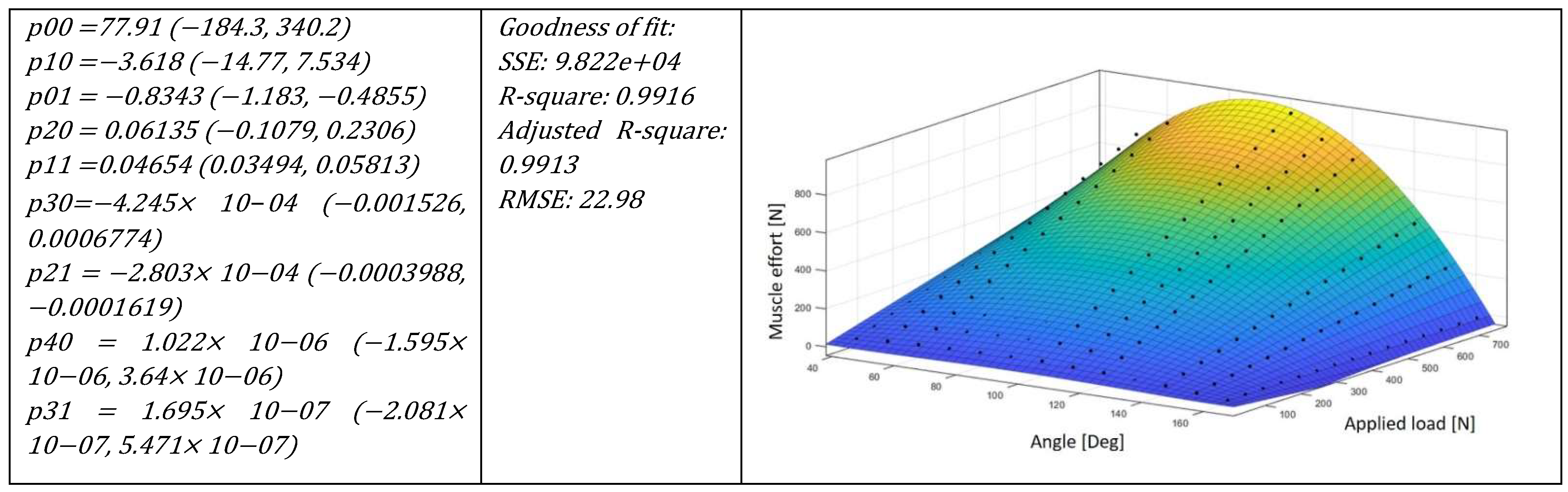
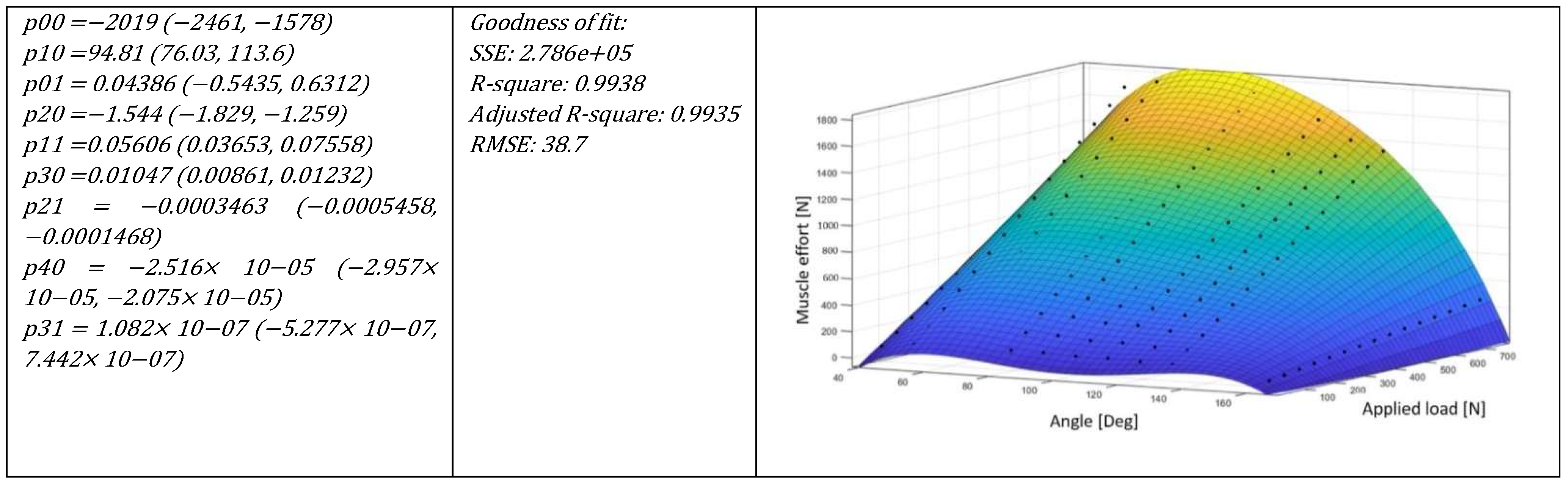
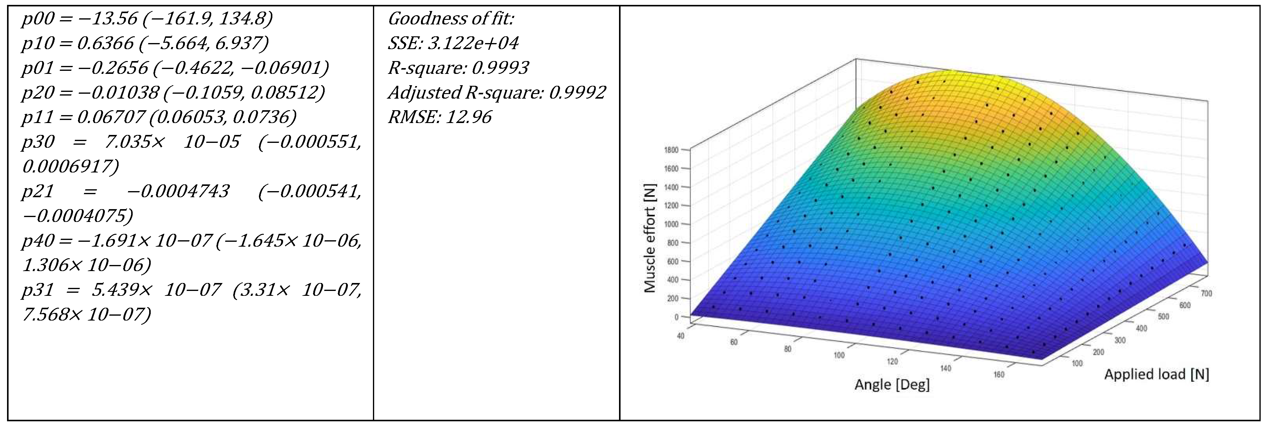
3.3.2. General Formulation

Applying the mathematical approach described above, equations of efforts for the five muscles involved will be presented, for any wrist load and elbow angle.

The approximation is done according to a fourth-grade polynomial with the general equation:

$$f\left(\alpha ,w\right)=p00+p10·\alpha +p01·w+p11·w·\alpha +p20·\alpha ^2+p21·w·\alpha ^2+p30·\alpha ^3+p31·w·\alpha ^3+p40·\alpha ^4$$

(12)

where α is the angle of the elbow and $w$ is the load applied to the wrist.

All coefficients have been calculated for a 95% confidence bound.

The surface of Figure 15 shows the tendency of the effort appearing in the short biceps muscle as a result of applying a vertical load on the wrist. As an example, for a constant vertical load of 750 N (including forearm mass), we could limit the short biceps effort to 200 N if we put the elbow joint angle between 150° to 164°.

In the range of the example of the previous figure, 150–164°, we could find an effort on long biceps bigger than in short biceps, reaching around 600 N. Figure 16, Figure 17, Figure 18 and Figure 19 collect the results of the surface reconstruction for the rest of studied muscles.

4. Discussion

In this study, an analytical calculation method is proposed to obtain the forces in the flexor muscles (long and short biceps) and extensors (long, lateral, and middle triceps) in any configuration of the opening angle of the elbow joint and to any load applied to the wrist. The final objective of this study is to allow the creation of a new type of finite element that can be included in a musculoskeletal model that can be analyzed in different positions and configurations without the need to repeat the model meshing process.

There are several studies along the same lines. Therefore, Martinez [12] is focused on the analysis of a certain muscle in a certain load situation, analyzing what happens in the muscle itself. Islan et al. [14], are focused on the muscles involved in the shoulder joint, under static condition predicting the fatigue and cumulative damage to the muscles. Alonso et al. [20] study the forces in the muscles involved in the human march under certain load conditions, weight and step frequency. Park et al. [22] develop a predictive method for muscle forces based on electromyography techniques. Teo et al. [26] are focused on the effect of a collision on the neck muscles. As can be seen, none of them addresses the problem from our perspective. The use of the finite element method is widely recognized as a calculation tool for structural, static, and/or dynamic problems. However, characterization of the muscle, so that it is easy to include it in an FEM model has not been addressed until now.

The main drawbacks presented by the studies carried out so far, in order to include the muscle in a valid finite element model to analyze the behavior of a muscle within a joint in various positions of this, are as follows:

• Studies have focused on one joint position, obtaining results related to muscle effort that are difficult to extrapolate to different positions. Ramírez [12] obtains the results for the anterior tibial muscle under study conditions, but moving the results to other load situations should be difficult to solve.
• The equations obtained to characterize the muscle are difficult to implement in a FEM model. Sachenkov et al. [29] use 1D elements to simulate muscles, but there is no single equation for any muscle to implement it in another analysis. The same happens with Alonso et al. [20], where the result is based on a static and physiological optimization that integrates the forces of any Hill MTU unit.
• Several of these studies use 3D elements to represent the muscle, which allows a better understanding of the internal behavior of the muscle itself (distribution of stresses and strains, deformations, etc.) but does not allow the created mesh to be reused in other positions of the joint. Therefore, Martínez [12] studies the anterior tibia muscle in a certain position, and if the muscle length changes, a new mesh should be developed. Another example is shown in research by Islan et al. [14], where they analyze the shoulder muscles of a violin player holding the instrument, and so, if the shoulder position changes, the mesh will do as well, remeshing the muscles into their new position.

With this work, and in a first approximation, we have obtained the equations that govern the behavior of the flexor and extensor muscles of the elbow, only in isometric contractions and referring to this behavior to its response in the form of force provided, throughout the flexion path of the joint for any load applied to the wrist.

For example, to calculate the estimated force that must appear in each of the joint muscles to support a load applied to the wrist of 235 N with the elbow forming an angle of 119 degrees, we need to substitute the values of α and $w$ in Equation (12), depending on which muscle we want to analyze.

Changing the indicated values in Equation (12) would obtain the following estimated forces in the muscles.

Vertical downward load, strength in Biceps muscles.

• Long biceps: 477 N;
• Short biceps: 245 N.

Upward vertical load, strength in the triceps muscles.

• Long triceps: 438 N;
• Middle triceps: 231;
• Side triceps: 304.

In addition to what has been said, the equations obtained to characterize the muscles in their response are easy to implement mathematically, which will undoubtedly help in the future in the possibility of creating a new type of finite element that responds to these behavioral equations obtained.

With the creation of this new type of finite element to represent muscles, a very interesting possibility is opened to analyze the behavior of the joint in different positions, with variable loads, different load cycles, etc. notably reducing the study work since the meshing process of the model is eliminated by being able to reuse the mesh for the desired positions.

Regarding the analysis of the results obtained, it is worth mentioning the following important aspects of the study.

Applying the proposed methodology and using the finite element method, we can obtain the forces that must appear in the muscles involved in the elbow joint to keep it in balance, in any position between 44 and 164 degrees of opening, with a load applied to the wrist of 150 N (Table 2, Figure 13 and Figure 14).

Through this same analysis it is possible to obtain the tensions that appear in the insertions of the tendons of the joint, which allows us to foresee damage before certain load situations (Figure 11 and Figure 12).

This same analysis allows us to obtain a map of tensions in the rigid tissues of the joint, bones, and cartilage. This allows a detailed study of damage to the elements mentioned (Figure 11 and Figure 12).

There are no previous studies that carry out studies similar to the proposed study, so a direct comparison with what has already been done is not possible. However, the trend observed in muscle effort during joint movement is similar to what other studies have published, [34], where the results of the torque in elbow vs. elbow angle shape are consistent with our results and [35] where the relation between the torque of the elbow and angle of the elbow is similar to our expressions, although these studies measure the moment in the joint (or what is the same, the sum of the moments generated by each muscle) and not the independent force in each muscle the results presented in these investigations are similar to those presented in this study in terms of the evolution of the moment in the joint, or of the force in the muscle in our case, along the angle of the joint.

The correlation also presents high R values, which confirms the validity of the analysis (Figure 13 and Figure 14).

Through the application of classical mechanics and the balance of forces and moments in the joint, we can extrapolate the results obtained for a specific load, 150 N in our case, to different loads applied to the joint (Figure 15, Figure 16, Figure 17, Figure 18 and Figure 19).

Finally, it should be mentioned that the equations that predict the force in each of the muscles in the joint are obtained as a function of the opening angle of the elbow and the applied load.

5. Conclusions

The use of a simplified model of the muscle, as a 1D element with axial forces only (ROD type element), into a FEA model allows one to calculate the forces that must be generated in the muscles involved in the joint.

It is also possible to predict the force required in each muscle for different load situations.

On the basis of the same analysis, the stresses that appear in other elements of the joint, bones, tendon insertions, or cartilage, can be obtained. With the obtained characteristic equations, different lines of research are opened focused on a better characterization of the muscles. It seems necessary to evolve the equations obtained in this study to obtain those that give the force of the muscle as a function of the speed of contraction. Or, based on studies conducted to assess muscle fatigue, they could be modified to predict it in a moving joint.

The evolution of this study should follow the following stages:

• Validation of the theoretical model obtained through testing with individuals with whom it is possible to measure the forces in cases of biceps and/or triceps load that, by means of comparison with this study, allows for knowing its validity.
• Modification of the equations obtained in this study in order to obtain their evolution for concentric or eccentric contractions.
• Creation of a new type of 1D element for application in finite element models that allows the behavior of a muscle to be characterized according to the equations obtained for any type of contraction, isometric, concentric, or eccentric.

Once these phases are completed, the work could be extrapolated to other types of muscle (flat, or peniform) in order to characterize more muscles that allow us to study new joints according to the proposed methodology.

One limitation of the presented study is the approximation of the muscle to the 1D element. This implies that following this methodology cannot obtain information regarding what happens inside the muscle.

Another one is that the analysis is performed for a certain size of elbow joint, and so the FEA model created is valid for this joint size; in any other case (children, older people, etc.), the FEA model should be resized, and the same methodology should be applied.

References

- Strouboulis, T.; Babuška, I.; Whiteman, J.R. The Finite Element Method and Its Reliability; Clarendon Press: Oxford, UK, 2001; ISBN 978-0-19-850276-0. [Google Scholar]
- Babuska, I.; Whiteman, J.; Strouboulis, T. Finite Elements: An Introduction to the Method and Error Estimation; OUP: Oxford, UK, 2010; ISBN 978-0-19-850669-0. [Google Scholar]
- Pawełko, P.; Jastrzębski, D.; Parus, A.; Jastrzębska, J. A new measurement system to determine stiffness distribution in machine tool workspace. Arch. Civ. Mech. Eng. 2021, 21, 49. [Google Scholar] [CrossRef]
- Wang, D.; Zhang, S.; Wang, L.; Liu, Y. Developing a Ball Screw Drive System of High-Speed Machine Tool Considering Dynamics. IEEE Trans. Ind. Electron. 2021, 69, 4966–4976. [Google Scholar] [CrossRef]
- Li, Z.; Oger, G.; Le Touzé, D. A partitioned framework for coupling LBM and FEM through an implicit IBM allowing non-conforming time-steps: Application to fluid-structure interaction in biomechanics. J. Comput. Phys. 2021, 449, 110786. [Google Scholar] [CrossRef]
- Della Rosa, N.; Bertozzi, N.; Adani, R. Biomechanics of external fixator of distal radius fracture, a new approach: Mutifix Wrist. Musculoskelet. Surg. 2020, 106, 89–97. [Google Scholar] [CrossRef] [PubMed]
- Zhang, N.-Z.; Xiong, Q.-S.; Yao, J.; Liu, B.-L.; Zhang, M.; Cheng, C.-K. Biomechanical changes at the adjacent segments induced by a lordotic porous interbody fusion cage. Comput. Biol. Med. 2022, 143, 105320. [Google Scholar] [CrossRef] [PubMed]
- Denozière, G.; Ku, D.N. Biomechanical Comparison between Fusion of Two Vertebrae and Implantation of an Artificial Intervertebral Disc. J. Biomech. 2006, 39, 766–775. [Google Scholar] [CrossRef] [PubMed]
- Samani, A.; Bishop, J.; Yaffe, M.J.; Plewes, D.B. Biomechanical 3-D finite element modeling of the human breast using MRI data. IEEE Trans. Med. Imaging 2001, 20, 271–279. [Google Scholar] [CrossRef]
- Jaecques, S.; Van Oosterwyck, H.; Muraru, L.; Van Cleynenbreugel, T.; De Smet, E.; Wevers, M.; Naert, I.; Sloten, J.V. Individualised, micro CT-based finite element modelling as a tool for biomechanical analysis related to tissue engineering of bone. Biomaterials 2003, 25, 1683–1696. [Google Scholar] [CrossRef]
- Renner, S.M.; Natarajan, R.N.; Patwardhan, A.G.; Havey, R.M.; Voronov, L.I.; Guo, B.Y.; Andersson, G.B.; An, H.S. Novel model to analyze the effect of a large compressive follower pre-load on range of motions in a lumbar spine. J. Biomech. 2007, 40, 1326–1332. [Google Scholar] [CrossRef]
- Martínez, A.M.R. Modelado y simulación del tejido músculo-esquelético. Validación Experimental con el Músculo Tibial Anterior de Rata. Ph.D. Thesis, Universidad de Zaragoza, Zaragoza, Spain, 2011. Available online: http://purl.org/dc/dcmitype/Text. (accessed on 5 November 2021).
- Weiss, J.A.; Gardiner, J.C.; Ellis, B.J.; Lujan, T.J.; Phatak, N.S. Three-dimensional finite element modeling of ligaments: Technical aspects. Med. Eng. Phys. 2005, 27, 845–861. [Google Scholar] [CrossRef]
- Islan, M.; Carvajal, J.; Pedro, P.S.; D’Amato, R.; Juanes, J.A.; Soriano, E. Linear Approximation of the Behavior of the Rotator Cuff under Fatigue Conditions. Violinist Case Study. In Proceedings of the ACM 5th International Conference on Technological Ecosystems for Enhancing Multiculturality, Cádiz, Spain, 18–20 October 2017; p. 58. [Google Scholar]
- Sachenkov, O.A.; Hasanov, R.F.; Andreev, P.S.; Konoplev, Y.G. Numerical Study of Stress-Strain State of Pelvis at the Proximal Femur Rotation Osteotomy. Russ. J. Biomech. 2016, 20, 220–232. [Google Scholar] [CrossRef]
- Martins, J.A.C.; Pato, M.P.M.; Pires, E.B. A finite element model of skeletal muscles. Virtual Phys. Prototyp. 2006, 1, 159–170. [Google Scholar] [CrossRef]
- Tang, C.; Tsui, C.; Stojanovic, B.; Kojic, M. Finite element modelling of skeletal muscles coupled with fatigue. Int. J. Mech. Sci. 2007, 49, 1179–1191. [Google Scholar] [CrossRef]
- Syomin, F.A.; Tsaturyan, A.K. Mechanical model of the left ventricle of the heart approximated by axisymmetric geometry. Russ. J. Numer. Anal. Math. Model. 2017, 32, 327–337. [Google Scholar] [CrossRef]
- Perreault, E.J.; Sandercock, T.G.; Heckman, C.J. Hill Muscle Model Performance during Natural Activation and Electrical Stimulation. In Proceedings of the 23rd Annual International Conference of the IEEE Engineering in Medicine and Biology Society, Istanbul, Turkey, 25–28 October 2001; Volume 2, pp. 1248–1251. [Google Scholar]
- Alonso, F.J.; Galán-Marín, G.; Salgado, D.R.; Pàmies Vilà, R.; Font Llagunes, J.M. Cálculo de Esfuerzos Musculares en la Marcha Humana Mediante Optimización Estática-Fisiológica. In Proceedings of the XVIII Congreso Nacional de Ingeniería Mecánica, Ciudad Real, Spain, 3–5 November 2010; pp. 1–9. [Google Scholar]
- Holzbaur, K.R.S.; Murray, W.M.; Delp, S.L. A Model of the Upper Extremity for Simulating Musculoskeletal Surgery and Analyzing Neuromuscular Control. Ann. Biomed. Eng. 2005, 33, 829–840. [Google Scholar] [CrossRef]
- Park, W.-I.; Lee, H.-D.; Kim, J. Estimation of isometric joint torque from muscle activation and length in intrinsic hand muscle. In Proceedings of the 2008 International Conference on Control, Automation and Systems, Seoul, Korea, 14–17 October 2008; pp. 2489–2493. [Google Scholar] [CrossRef]
- Soechting, J.F.; Flanders, M. Evaluating an Integrated Musculoskeletal Model of the Human Arm. J. Biomech. Eng. 1997, 119, 93–102. [Google Scholar] [CrossRef]
- Zajac, F.E. Muscle and Tendon: Properties, Models, Scaling, and Application to Biomechanics and Motor Control. Crit. Rev. Biomed Eng. 1989, 17, 359–411. [Google Scholar]
- Lechosa Urquijo, E.; Blaya Haro, F.; D’Amato, R.; Juanes Méndez, J.A. Finite Element Model of an Elbow under Load, Muscle Effort Analysis When Modeled Using 1D Rod Element. In Proceedings of the Eighth International Conference on Technological Ecosystems for Enhancing Multiculturality, Salamanca, Spain, 21–23 October 2020; Association for Computing Machinery: New York, NY, USA, 21 October 2020; pp. 475–482. [Google Scholar]
- Teo, E.C.; Zhang, Q.H.; Qiu, T.X. Finite Element Analysis of Head-Neck Kinematics Under Rear-End Impact Conditions. In Proceedings of the 2006 International Conference on Biomedical and Pharmaceutical Engineering, Singapore, 11–14 December 2006; pp. 206–209. [Google Scholar]
- Donahue, T.L.H.; Hull, M.L.; Rashid, M.M.; Jacobs, C.R. A Finite Element Model of the Human Knee Joint for the Study of Tibio-Femoral Contact. J. Biomech. Eng. 2002, 124, 273–280. [Google Scholar] [CrossRef]
- Abidin, N.A.Z.; Kadir, M.R.A.; Ramlee, M.H. Three Dimensional Finite Element Modelling and Analysis of Human Knee Joint-Model Verification. J. Phys. Conf. Ser. 2019, 1372, 012068. [Google Scholar] [CrossRef]
- Sachenkov, O.A.; Hasanov, R.; Andreev, P.; Konoplev, Y. Determination of Muscle Effort at the Proximal Femur Rotation Osteotomy. IOP Conf. Series: Mater. Sci. Eng. 2016, 158, 012079. [Google Scholar] [CrossRef] [Green Version]
- Jesal, N. Parekh Using Finite Element Methods to Study Anterior Cruciate Ligament Injuries: Understanding the Role of ACL Modulus and Tibial Surface Geometry on ACL Loading. Ph.D. Thesis, The University of Michigan, Ann Arbor, MI, USA, 2013. [Google Scholar]
- CES EduPack Bulletin: January 2017. Available online: https://www.grantadesign.com/newsletters/ces-edupack-bulletin-ces-edupack-2017-new-products-database-symposia-deadlines-shared-resources-webinars-and-more/ (accessed on 20 June 2022).
- Bruno, S.; José, M.; Filomena, S.; Vítor, C.; Demétrio, M.; Karolina, B. The Conceptual Design of a Mechatronic System to Handle Bedridden Elderly Individuals. Sensors 2016, 16, 725. [Google Scholar] [CrossRef] [PubMed] [Green Version]
- Arcila Arango, J.C.; Cardona Nieto, D.; Giraldo, J.C. Abordaje Físico-Matemático Del Gesto Articular. Available online: https://www.efdeportes.com/efd171/abordaje-fisico-matematico-del-gesto-articular.htm (accessed on 5 November 2021).
- Loss, J.F.; Candotti, C.T. Comparative Study between Two Elbow Flexion Exercises Using the Estimated Resultant Muscle Force. Braz. J. Phys. Ther. 2008, 12, 502–510. [Google Scholar] [CrossRef] [Green Version]
- Murray, W.M.; Delp, S.L.; Buchanan, T.S. Variation of Muscle Moment Arms with Elbow and Forearm Position. J. Biomech. 1995, 28, 513–525. [Google Scholar] [CrossRef]