Hybridization of Manta-Ray Foraging Optimization Algorithm with Pseudo Parameter-Based Genetic Algorithm for Dealing Optimization Problems and Unit Commitment Problem

Abstract

The manta ray foraging optimization algorithm (MRFO) is one of the promised meta-heuristic optimization algorithms. However, it can stick to a local minimum, consuming iterations without reaching the optimum solution. So, this paper proposes a hybridization between MRFO, and the genetic algorithm (GA) based on a pseudo parameter; where the GA can help MRFO to escape from falling into the local minimum. It is called a pseudo genetic algorithm with manta-ray foraging optimization (PGA-MRFO). The proposed algorithm is not a classical hybridization between MRFO and GA, wherein the classical hybridization consumes time in the search process as each algorithm is applied to all system variables. In addition, the classical hybridization results in an extended search algorithm, especially in systems with many variables. The PGA-MRFO hybridizes the pseudo-parameter-based GA and the MRFO algorithm to produce a more efficient algorithm that combines the advantages of both algorithms without getting stuck in a local minimum or taking a long time in the calculations. The pseudo parameter enables the GA to be applied to a specific number of variables and not to all system variables leading to reduce the computation time and burden. Also, the proposed algorithm used an approximation for the gradient of the objective function, which leads to dispensing derivatives calculations. Besides, PGA-MRFO depends on the pseudo inverse of non-square matrices, which saves calculations time; where the dependence on the pseudo inverse gives the algorithm more flexibility to deal with square and non-square systems. The proposed algorithm will be tested on the test functions that the main MRFO failed to find their optimum solution to prove its capability and efficiency. In addition, it will be applied to solve the unit commitment (UC) problem as one of the vital power system problems to show the validity of the proposed algorithm in practical applications. Finally, several analyses will be applied to the proposed algorithm to illustrate its effectiveness and reliability.

1. Introduction

The optimization problem is finding the optimal set of control variables, whether continuous or discrete. Accordingly, the optimization problems can be classified into; discrete or continuous. Constrained and multimodal problems are examples of optimization problems [1,2].

The optimization problems are highly significant from both the manufacturing and scientific perspective. It is a vital and challenging area, especially in engineering designs that have efficient form and are more accurate. Besides, the feasible region may be a narrow subset of the search domain. Also, according to the presence or absence of equality or inequality constraints, optimization problems are categorized into constrained and unconstrained problems. Traditionally, for the unconstrained optimization problems, many techniques were classified into direct search and gradient-based methods. While the constrained optimization problems algorithms are classified into indirect and direct methods. These traditional optimization techniques are insufficiently robust in discontinuous, vast multimodal, and noisy search spaces [3,4].

Due to the shortcomings of traditional optimization approaches, meta-heuristic techniques have been introduced for handling optimization problems. Meta-heuristic algorithms are the most exemplary optimization algorithms due to their robustness, performance reliability, simplicity, and ease of implementation, among other benefits. There are various types of meta-heuristic algorithms, including:

(1) Evolutionary algorithms: These algorithms, such as the genetic algorithm (GA) [5,6,7,8], differential evolution algorithm (DEA) [9], and evolutionary strategy algorithm (ESA) [10], are based on evolutionary theory. The evolutionary algorithms apply the search during simulation of the inspired process by selection and reproduction, to find the optimum solution. They are global optimization methods, that scale well to higher-dimensional problems, as they are robust concerning noisy evaluation functions. However, they may not find the global optimum solution, can stick to a local minimum and consume iterations without improvement, and require relatively high computational.

(2) Swarm-based algorithms: Swarm-based algorithms are considered the most basic forms of meta-heuristic algorithms. These algorithms modeled the behavior and characteristics of swarms’ systems, leading to the coining of the term “swarm intelligence” (SI) by Gerardo Beni and Jing Wang in 1989 [11]. Swarm intelligence algorithms (SIAs) are linked to the study of swarms, or colonies of social animals, where research into social behavior in swarms of organisms encouraged the invention of several practical optimization algorithms. These algorithms simulate the social behavior and decision-making of various social groupings, such as particle swarm optimization algorithm (PSOA), ant colony optimization algorithm (ACOA), grasshopper optimization algorithm (GOA), and manta-ray foraging optimization algorithm (MRFOA) [12,13,14,15,16,17], etc. There are several advantages to swarm-based algorithms such as they respond to internal disturbances and external challenges and complete operations even with the failure of some agents. Also, they are self-organized, which means that the solutions are emergent than pre-defined. Furthermore, the swarm system is updated based on predetermined and new stimuli, and the agents’ operations are implemented in a parallel manner. However, they have some drawbacks: the swarm’s function cannot be predicted according to the agent’s function. In addition, it is difficult to predict the behavior from the individual rules. Besides, they are sensitive to small changes in their laws where any change could lead to an unexpected group level.

(3) Human social behavior-based algorithms: These algorithms are based on human social behavior, such as group teaching optimization algorithm (GTOA), imperialist competitive algorithm (ICA), and teaching-learning based optimization algorithm [18,19,20,21,22], etc. These types of algorithms allow the social phenomena to be a valuable source of inspiration for algorithms. The efficiency and effectiveness of these algorithms may be better than other swarm intelligent mechanisms that animal groups inspire. However, they have the same drawbacks as swarm-based algorithms.

(4) Physics-based algorithms: Natural physics laws have been utilized to develop physics-based algorithms such as the gravitational search algorithm (GSA) [23], magnetic optimization algorithm (MOA) [24], and the simulated annealing (SA) [25], etc. In the GSA algorithm, according to Newton’s universal law of gravitation, larger particles will have more attraction power than smaller particles. Hence, smaller ones are attracted to the larger ones. Consequentially, all smaller particles will be drawn toward the largest particle. The largest particle can resemble the global optimum solution in the case of optimization. While the probable solutions in the MOA are magnetic particles distributed throughout the search space. According to its fitness, each magnetic particle has a mass and magnetic field measurement. Magnetic particles with a larger magnetic field and mass are more suitable. These particles live in a lattice-like environment and attract their neighbors with a force of attraction. The proposed cellular structure allows for greater exploitation of local neighborhoods before they progress to the global best, increasing population variety. Also, SA [25] is one of the physics-based popular algorithms. SA is a random-search technique that simulates how a metal cools and freezes into a minimum energy crystalline structure (the annealing process) and searches for a minimum in a system. These algorithms can deal with arbitrary systems and cost functions, almost guarantee to find an optimal solution, and are relatively easy to code, even for complex problems. However, these metaheuristic algorithms require many choices to turn them into actual algorithms. Besides, they may become very slow, especially if the cost function is expensive to compute. The precision of the numbers used in implementing these algorithms can significantly affect the speed and ability to reach the solution.

The MRFO algorithm [17] is a bio-inspired swarm intelligence optimizer that simulates the food search proclivities of the manta ray. According to three inclinations, Manta ray searches for food: chain foraging, cyclone foraging, and somersault foraging. Foraging manta rays line up in an organized manner to capture lost prey missed or undetected by the last manta ray in the chain in a process known as chain foraging. This cooperative interaction between competing manta rays reduces the possibility of prey loss in their eyesight and increases food rewards. Foraging by a cyclone occurs when there is a high density of prey.

However, MRFO is not good at fine-tuning solutions around optima due to its stochastic nature and slow convergence speed. Also, it may stick to a local minimum, leading to consuming iterations without reaching the optimal solution. Due to the above drawbacks, several modifications were applied to MRFO to enhance its performance. The combination of the SA and MRFO algorithms is presented in [26]; where the SA algorithm is used to describe the initial population of the MRFO algorithm, which speeds up convergence significantly. However, falling into a local minimum still represents a critical issue in the algorithm. In [27], an elegant approach is proposed based on MRFO integrated with a gradient-based optimizer (GBO). The proposed MRFO-GBO aims to decrease the risk of the original MRFO being stuck in local optima while also speeding up the solution process. It depends on a local escaping operator (LEO) to update the current solution. However, the LEO operator generates a new solution using several solutions (the best and other randomly selected solutions), which does not guarantee a better solution. In [26], the opposition-based learning (OBL) methodology was combined with MRFO to obtain an appropriate structure for optimization problems. The hybrid algorithm aimed to benefit from OBL to produce a more performant algorithm. However, it depends on computing all the population’s opposite solutions, and consequently, the computational load increases.

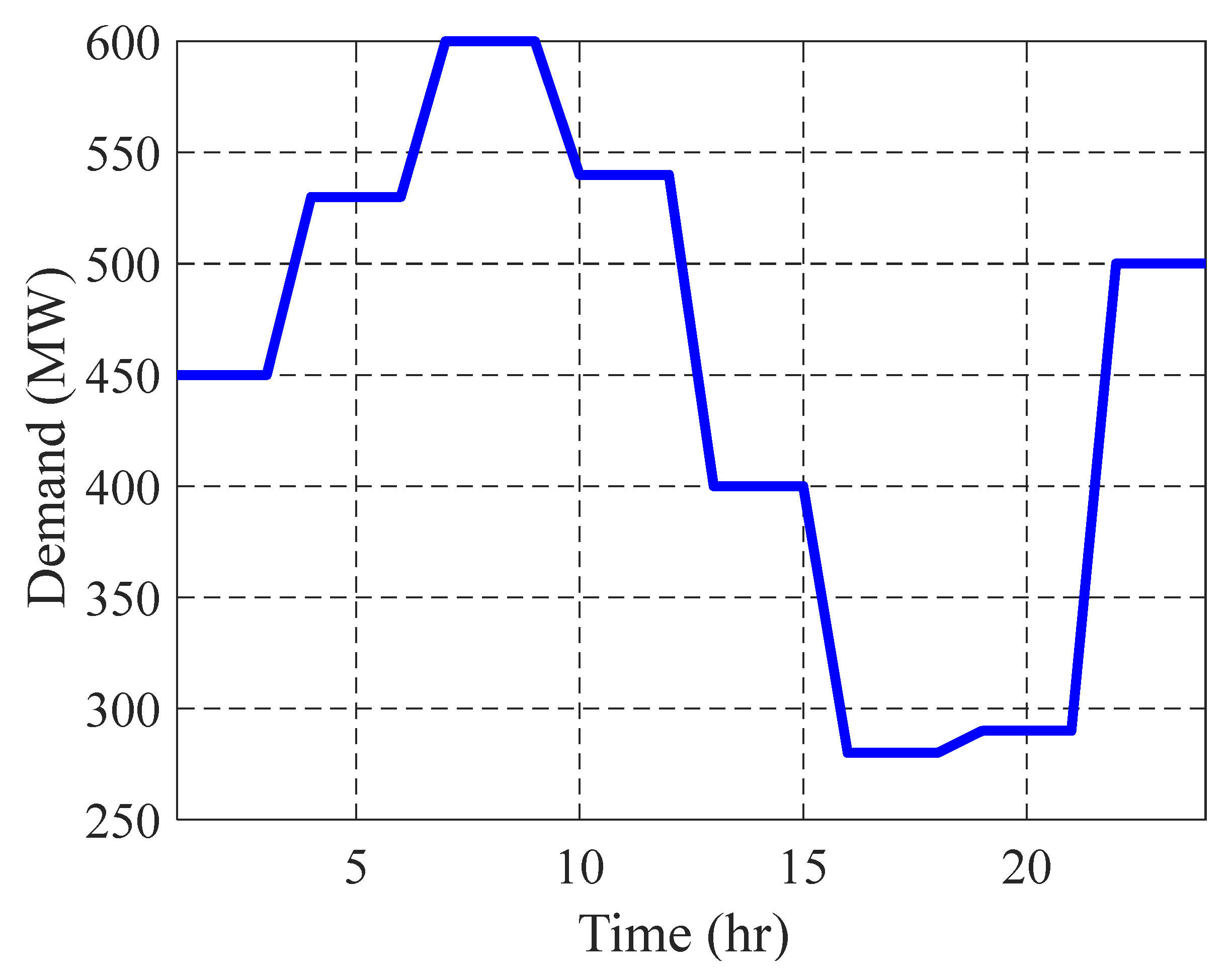
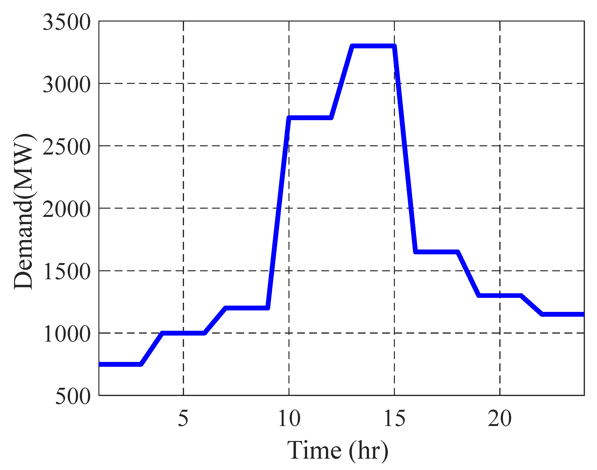
The ‘unit commitment’ (UC) problem in power systems aims to determine the startup and shut down schedules of generating units to meet forecasted demands over a definite period. The objective is to minimize the total production cost while satisfying all problem constraints. The global optimum solution can be obtained by exploring all possible solutions and choosing the one having the minimum objective value. However, in realistic power systems, this is not applicable. Therefore, researchers used different algorithms to find a satisfactory solution to achieve the constraints and objectives within a reasonable time [28].

Various approaches and several mathematical techniques have been proposed for solving the UC problem. Several inspired algorithms were applied to solve the UC problem due to their capability to handle nonlinear, mixed-integer, and large-scale problems. Besides, they can manage non-convex fuel cost functions with non-linear constraints. Some of the most commonly used algorithms are artificial neural network [29], simulated annealing [30], grey wolf optimizer [31], genetic algorithm, and particle swarm optimization technique [32,33]. Also, hybrid meta-heuristic optimization techniques have been applied to the UC problem considering the advantages and features of each optimization technique [34,35].

To improve the standard MRFO performance, this paper presents a hybridization of the manta-ray foraging optimization (MRFO) algorithm with a pseudo-parameter-based genetic algorithm (GA). The proposed algorithm is abbreviated as PGA-MRFO. The proposed algorithm applies the MRFO with its classical procedure until it is stuck in a local minimum. Then, the assumption of the pseudo parameter is used, leading to reducing the number of input variables in the GA. Finally, the GA will be applied to get out of the local minimum. Then, the assumption of the pseudo parameter is used, leading to reducing the number of input variables in the genetic algorithm. Finally, the GA will be applied to get out of the local minimum. Then, the search process will continue using the classical MRFO until it falls into a local minimum again. These processes are continued until the termination criterion is satisfied, at which point the best manta ray is reported as the final solution. The main contributions of the proposed algorithm can be summarized as follows:

• The manta-ray foraging optimization (MRFO) technique is proposed to be combined with a pseudo-parameter-based genetic algorithm (GA) to overcome and improve the poor performance of standard MRFO.
• The GA’s objective function depends only on three variables, whatever the number of independent variables in the problem. The dimension of the optimization problem will not affect the number of the GA’s variables leading to less computational burden.
• The suggested approach uses GA to take out the manta-ray algorithm from any local minimum to a better local minimum until an optimal solution is found.

The rest of the paper is organized as follows: Section 2 represents an overview of the MRFO algorithm. Section 3 illustrates the proposed algorithm with its flowchart and pseudo-code. Section 4 shows the results and comparisons based on five test functions. A practical application of the proposed algorithm to solve one of the most critical issues in the electrical power systems (unit commitment) problem is introduced in Section 5. Section 6 presents the proposed algorithm’s uncertainty, robustness, and computational time analysis. Finally, Section 7 introduces the conclusion.

2. MRFO Overview

Manta beams are extravagant animals. However, they have all the earmarks of being horrible. A grown-up manta beam can eat 5 kg of tiny fish regularly. They have developed an assortment of unique and astute scrounging methodologies. The primary scavenging technique is chain searching. When at least 50 manta beams begin scrounging, they line up, one behind another, shaping a precise line. More modest male manta beams are piggybacked upon female ones and swim on top of their backs to coordinate with the beats of the female’s sectoral balances. The second searching system is tornado scavenging.

Many manta beams assemble when the centralization of tiny fish is exceptionally high. Their last parts interface up with heads in twisting to create a spiraling vertex in the eye of the twister, and the separated water climbs towards the surface, which maneuvers the microscopic fish into their open mouths. The final foraging strategy is somersault foraging. Its behavior is one of the most splendid sceneries in nature. When manta rays find a food source, they will do a series of backward somersaults, circling the plankton to draw it towards manta rays. Somersault is a random, frequent, local and cyclical movement that helps manta rays optimize food intake.

In MRFO, manta rays can observe the position of plankton and swim towards it. The higher the concentration of plankton in a place, the better the situation is. Although the best solution is unknown, MRFO assumes the best solution found so far is the plankton with a high concentration of manta rays that want to approach and eat. Manta rays line up head-to-tail and form a foraging chain. Individuals except for the first move towards the food and the one in front of it. In each iteration, the individual is updated by the best solution and the solution in front of it. Chain individual foraging can be modeled as follows:

$$x_i^d\left(t+1\right) \{\begin{array}{c}{x}_i^d\left(t\right)+r\times \left(x_{best}^d\left(t\right)-x_i^d\left(t\right)\right)+{\alpha }_1\left(x_{best}^d\left(t\right)-x_i^d\left(t\right)\right), i=1\\ x_i^d\left(t\right)+r\times \left(x_{i-1}^d\left(t\right)-x_i^d\left(t\right)\right)+{\alpha }_1\left(x_{best}^d\left(t\right)-x_i^d\left(t\right)\right), i=2,3,\dots N\end{array}$$

(1)

$${\alpha }_1=2r\sqrt{\left|\log r\right|}$$

(2)

The position update of the ith individual is determined by the position $x_{i-1}^d\left(t\right)$ of the (i−1) the current individual and the position $x_{best}^d\left(t\right)$ of the food. When a school of manta rays recognizes a patch of plankton in deep water, they will form a long foraging chain and swim towards the food by a spiral. A similar spiral foraging strategy can be found in WOA. In the cyclone foraging strategy, each manta ray swims toward the one in front of it. The manta ray swarms in line, developing a spiral perform foraging. Individual not only follow the one in front of it but only moves toward the food along a spiral path. This motion behavior may be extended to an n-D space. For simplicity, this mathematical model of cyclone foraging can be defined as:

$$x_i^d\left(t+1\right) \{\begin{array}{c}{x}_{best}^d\left(t\right)+r\times \left(x_{best}^d\left(t\right)-x_i^d\left(t\right)\right)+\beta \left(x_{best}^d\left(t\right)-x_i^d\left(t\right)\right), i=1\\ x_{best}^d\left(t\right)+r\times \left(x_{i-1}^d\left(t\right)-x_i^d\left(t\right)\right)+\beta \left(x_{best}^d\left(t\right)-x_i^d\left(t\right)\right), i=2,3,\dots N\end{array}$$

(3)

$$\beta =2e^{\frac{r_1\left(T-t+1\right)}{T}} \sin \left(2\pi r_1\right)$$

(4)

In somersault foraging behavior, the position of the food is viewed as a pivot. Each individual swims to and from around the pivot and somersaults to a new position. Therefore, they constantly update their positions around the best position. The mathematical model can be created as follows:

$$x_i^d\left(t+1\right)=x_i^d\left(t\right)+S (r_2{x}_{best}^d\left(t\right)-r_3{x}_i^d\left(t\right))$$

(5)

MRFO starts by generating a random population in the problem domain as with other metaheuristic optimizers. Each updates its position according to the one in front of it and the reference position at each iteration. The value of the ratio increases from $\left(\frac{1}{T}\right)$ to 1, respectively, perform the exploratory and exploitative search. The current best solution is chosen as a reference for exploitation when the ratio $\left(\frac{t}{T}\right)<random number$. However, when the ratio $\left(\frac{t}{T}\right)>random number$, a random position in the search space, is selected as a reference position for the exploration.

Meanwhile, MRFO can switch between the chain foraging behavior and the cyclone foraging behavior according to the random number. Then individuals update their positions concerning the best position found so far by somersault foraging. All the updates and calculations are interactively performed until the stop criterion is met. Eventually, the best individual’s position and fitness value are returned. Algorithm 1 illustrates the pseudo-code of the MRFO algorithm.

Algorithm 1. Pseudo-code of MRFO algorithm.

According to the MRFO algorithm procedure, the best solution will not be updated if the current fitness function is not better than the previous iteration. Consequently, the algorithm will be stuck in the reached local point. As a result, an additional procedure should be applied to get it out from this local minimum point.

3. The Proposed Algorithm (PGA-MRFO)

3.1. Flow Chart and General Description of the Algorithm

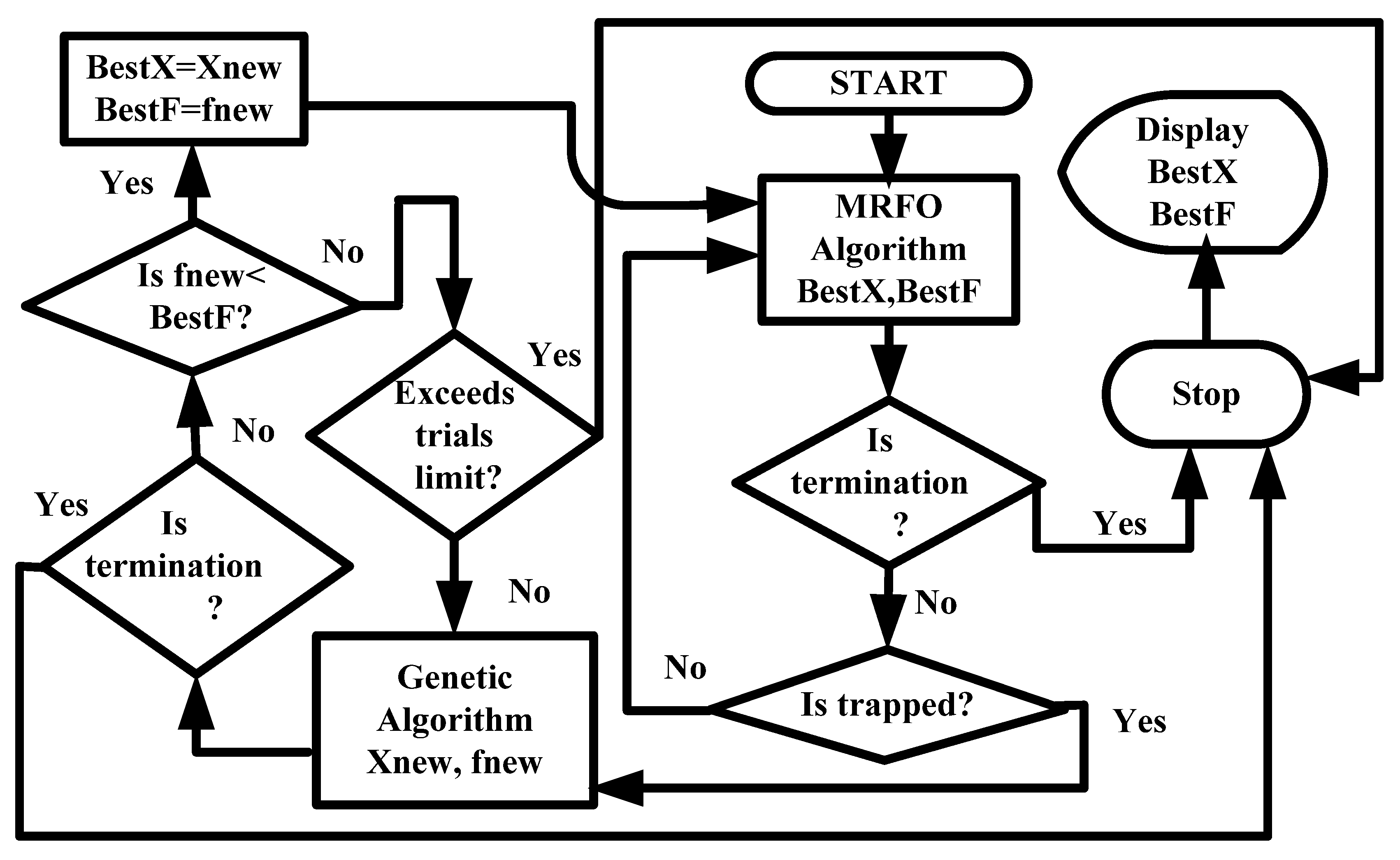
Figure 1 shows the flow chart of the proposed algorithm. The MRFO is applied until it falls into a local minimum point. Then, the genetic algorithm (GA) is used according to specific variables and the objective function until a better solution is obtained. The resulting solution and corresponding objective value are entered into the MRFO as the best solution and fitness function to complete the optimization process. The fundamental steps are repeated until the termination criterion is reached.

3.2. Mathematical Formulation of the Genetic Objective Function

Each variable in the system can be represented as a function of a parameterization parameter (s); each variable can be written as:

$$x_i=g_i\left(s\right), for i=1,\dots ,N$$

(6)

Also, the objective function can be stated as a function of the parameterization variable. It can be written as:

$$X=\left[x_1 x_2\dots x_N\right] , for i=1,\dots ,N$$

(7)

$$f=f\left(X\right)=f\left(g_i\left(s\right)\right).$$

(8)

Let

$$x_i\in \left[a_i, b_i\right] for i=1,2,\dots ,N$$

(9)

Then, the domain of parameterization parameter can be estimated as:

$$s\in \left[s_{min}, s_{max}\right]$$

(10)

where

$$s_{min}=\min \left\{a_1, a_2,\dots ,a_N\right\}$$

(11)

$$s_{max}=\max \left\{b_1, b_2,\dots ,b_N\right\}$$

(12)

Consequently,

$$\Delta s\in \left[s_{min}, s_{max}\right]$$

(13)

Equation (13) states that the parameterization parameter domain is bounded by the minimum and maximum values of lower and upper limits of the system variables, respectively.

Theorem 1.

(First Order Necessary Condition for (Local) Optimality) [2].

If $X$ is an unconstrained local minimizer of a differentiable function, then we must have According to the First Order Necessary Condition for (Local) Optimality) If $X$ is an unconstrained local minimizer of a differentiable function $f: R^N\to R$, then:

$$\nabla f\left(X\right)=0$$

(14)

The derivative of the fitness function WRT, the parameterization parameter, can be written as:

$$\frac{df}{ds}=\frac{df}{d{g}_1}\times \frac{d{g}_1}{ds}+\frac{df}{d{g}_2}\times \frac{d{g}_2}{ds}+\dots +\frac{df}{d{g}_N}\times \frac{d{g}_N}{ds}$$

(15)

According to Equation (6), Equation (15) can be written as:

$$\frac{df}{ds}=\frac{df}{d{x}_1}\times \frac{d{x}_1}{ds}+\frac{df}{d{x}_2}\times \frac{d{x}_2}{ds}+\dots +\frac{df}{d{x}_N}\times \frac{d{x}_N}{ds}$$

(16)

As a vector form, Equation (16) can be written as:

$$\frac{df}{ds}=\left[\frac{df}{d{x}_1} \frac{df}{d{x}_2} \dots \dots \frac{df}{d{x}_N}\right]\times \left[\begin{array}{c}\frac{d{x}_1}{ds}\\ \frac{d{x}_1}{ds}\\ ..\\ ..\\ \frac{d{x}_N}{ds}\end{array}\right]$$

(17)

The first vector represents the gradient of the objective function to the system variables. So, Equation (17) can be written as:

$$\frac{df}{ds}=\nabla f\times \left[\begin{array}{c}\frac{d{x}_1}{ds}\\ \frac{d{x}_1}{ds}\\ ..\\ ..\\ \frac{d{x}_N}{ds}\end{array}\right]$$

(18)

where,

$$\nabla f=\left[\frac{df}{d{x}_1} \frac{df}{d{x}_2} \dots \dots \frac{df}{d{x}_N}\right]$$

(19)

According to the previous theorem, the gradient of Equation (19) can be approximated as:

$$\nabla f=\alpha \left[c_1 c_2\dots \dots c_N\right]$$

(20)

where,

$$c_i\in \left[0,1\right]$$

(21)

$$\alpha \in \left[-{10}^{-6}, {10}^{-6}\right]$$

(22)

According to Equation (18), the gradient of the variables w.r.t. the parameterization parameter $\left(\mathsf{\Delta }X\right)$ can be calculated as:

$$\{\begin{array}{c}\frac{\mathsf{\Delta }X}{\Delta s}=\left[\begin{array}{c}\frac{d{x}_1}{ds}\\ \frac{d{x}_2}{ds}\\ ..\\ ..\\ \frac{d{x}_N}{ds}\end{array}\right]=\frac{df}{ds}\times {(\nabla f)}^{+}=\frac{\Delta f}{\Delta s}\times {(\nabla f)}^{+}\\ \Delta x=\frac{\Delta x}{\Delta s}\times \Delta s\end{array}$$

(23)

$$\frac{df}{ds}=\frac{\Delta f}{\Delta s}$$

(24)

where ${(\nabla f)}^{+}$ is the pseudo-inverse (Moore-Penrose) of the approximated gradient. The resulting objective function from the GA should be less than the entered one. It can be written as:

$$\Delta f=\{\begin{array}{c}\delta f-f if f\ge 0\\ \\ f-\frac{f}{\delta } if f<0\end{array} \mathrm{where} \delta \in \left(0,1\right)$$

(25)

$$X=\left[x_1 x_2\dots \dots x_N\right], for i=1,\dots ,N;$$

(26)

After calculating the gradient ($\mathsf{\Delta }X)$. The updated values of the variables can be evaluated as:

$$X_n=X+\Delta X^T=\left[x_1 x_2\dots \dots x_N\right]+\left[\frac{d{x}_1}{ds} \frac{d{x}_2}{ds}\dots \dots \frac{d{x}_N}{ds}\right]$$

(27)

$$X_{new}=corecteion \left(X_n\right)$$

(28)

Then, the fitness function of the new individual can be calculated as:

$$f_{new}=f\left(X_{new}\right)$$

(29)

So that the variables of the GA will be {$\delta , \Delta s, \alpha$}.

The GA aims to reduce the absolute difference between the calculated fitness function of the new solution ($f_{new})$ and the presumed enhanced fitness function ($\delta f or \frac{f}{\delta })$. The fitness function in the GA can be written as follows:

$$fitness \left(X\right)=\{\begin{array}{c}\left|f_{new}-\delta f\right| if f\ge 0\\ \\ \left|f_{new}-\frac{f}{\delta }\right| if f<0\end{array}$$

(30)

The whole optimization problem that is presented to the GA is as follows:

$$\left\{\begin{array}{c}\underset{\alpha \in \left[-{10}^{-6}, {10}^{-6}\right], \delta \in \left(0,1\right) , \Delta s\in \left[\mathit{tan}-\frac{\pi }{2}, \mathit{tan}\frac{\pi }{2}\right]}{\min }\left|f_{new}-\delta f\right| if f\ge 0\\ \underset{\alpha \in \left[-{10}^{-6}, {10}^{-6}\right], \delta \in \left(0,1\right) , \Delta s\in \left[\mathit{tan}-\frac{\pi }{2},\mathit{tan}\frac{\pi }{2}\right]}{\min }\left|f_{new}-\frac{f}{\delta }\right| if f<0\end{array}\right\}$$

(31)

The GA is applied based on the objective function in Equation (31) through the defined domain. If the enhanced solution is obtained, the genetic operations are terminated, and the resulted solution with its objective function is reintroduced to the MRFO algorithm. Otherwise, the GA continues based on the resulting solution until getting an enhanced solution and getting out of the local minimum point.

3.3. Detailed Steps of the Proposed Algorithm (PGA-MRFO)

In this section, the detailed steps of the proposed algorithm are explained.

Step 1: The MRFO is applied with its standard procedure until the termination condition, or it cannot update the best solution of the current iteration, which means falling into a local minimum.

Step 2: The GA is initialized with the best solution resulting from MRFO, the number of populations and generations, the domain of the genetic variables ($\alpha , \delta ,\Delta s),$ and other genetic parameters. Then, the initial population of the GA is created.

Step 3: For each individual, the new solution is calculated according to Equations (27) and (28). Then, its objective function is calculated according to Equation (29), and the corresponding fitness function of the GA is calculated according to Equation (30).

Step 4: The rest of the GA’s operations continue until the maximum number of generations is terminated. The best solution yielded from the GA ($X_{new}, f_{new})$ will satisfy one of the following three cases.

(a)

It may satisfy the problem’s termination (stopping) criterion. Then, it will be approved as the optimum solution, and the search process will be terminated.

(b)

If it is better than the trapped solution of MRFO, it will replace the MRFO’s trapping solution, and the MRFO algorithm is reapplied.

(c)

Suppose the resulting solution is not better than the trapped solution of MRFO. In that case, it will be entered again into the GA to be improved according to the genetic objective function (step 2).

Step 5: Steps 1–4 are repeated until the termination (stopping) criterion is reached.

For further illustrations of the PGA-MRFO, the pseudo-code is detailed in Algorithm 2.

Algorithm 2. Pseudo-code of PGA-MRFO.

Step 6: This step is added to avoid cycling if the GA fails to enhance the existing solution. The GA trials’ limit will be defined in the PGA-MRFO algorithm. If the GA fails to improve the solution in the current trial, its last population will be used as the initial population for the subsequent trial. Suppose the trial number exceeds the GA trials’ limit. In that case, the algorithm terminates, and the PGA-MRFO returns the best-calculated solution and its corresponding objective value as the local optimum solution to that problem. The GA trials’ limit is 5 in the proposed algorithm.

4. Testing Performance of PGA-MRFO Algorithm

The proposed algorithm was coded in MATLAB. 2020a, implemented with a Core (TM) i7, Intel(R) CPU with 3.2 GHz and 16 GB RAM. For computational studies, a population size of 50 and 1000 generations is used, the crossover fraction is 0.8, and all other parameters and functions were default as in GA Tool. Also, the termination criterion for both algorithms (MRFO and PGA-MRFO) is defined as $\delta =\left|\Vert F_{optimum}\Vert -\Vert F_l\Vert \right|\le Tolerence$= 1 × 10⁻⁶; where $F_{optimum}$ is the optimal objective of the test function, and $F_l$ is the calculated objective by the algorithm.

According to the MRFO test functions in [18], ten test functions (F₅, F₇, F₈, F₁₃, F₁₄, F₁₅, F₂₀, F₂₁, F₂₂, and F₂₃) fall into a local minimum. So, both classical MRFO and PGA-MRFO algorithms will be applied to these ten test functions to verify the validation and reliability of the proposed (PGA-MRFO) algorithm. The results of each algorithm will be compared to the optimum solution based on the stopping criterion.

Table 1. Comparison between the two algorithms according to the consumed iterations.

Test Function	Function No.	D	Domain	NO. of Iterations Using MRFO	NO. of Iterations Using PGA-MRFO	Percentage Improvement
Rosenbrok	F5	30	$\left[-30,30\right]$	1000	438	56.2%
Quartic	F7	30	[−1.28,1.28]	1000	419	58.1%
Schwefel	F8	30	$\left[-500,500\right]$	1000	520	48%
Penalized2	F13	30	[−50,50]	1000	181	81.9%
Foxholes	F14	2	[−65.536,65.536]	62	42	32.2%
Kowalik	F15	4	[−5,5]	1000	169	83.1%
Hartman 6	F20	6	[0,1]	500	35	93%
Shekel 5	F21	4	[0,10]	1000	109	89.1%
Shekel 7	F22	4	[0,10]	325	165	49.2%
Shekel 10	F23	4	[0,10]	1000	87	91.3%

compares the two algorithms according to the number of consumed iterations. In all test functions, the PGA-MRFO outperformed the conventional MRFO in achieving a lower value for F_best in fewer iterations, except for F₈, where it reached a better value for F_best in the same number of iterations, as shown in Table 1. The results illustrate how the PGA-MRFO converged faster and was more reliable than the original MRFO. Table 1’s last column indicates the suggested algorithm’s improvement as a percentage relation, which is determined as follows:

$$\mathrm{Percentage} \mathrm{improvement}=\frac{\left|\mathrm{PGA}-\mathrm{MRFO} \mathrm{iterations}-\mathrm{MRFO} \mathrm{iterations}\right|}{\mathrm{MRFO} \mathrm{iterations}}\times 100.$$

(32)

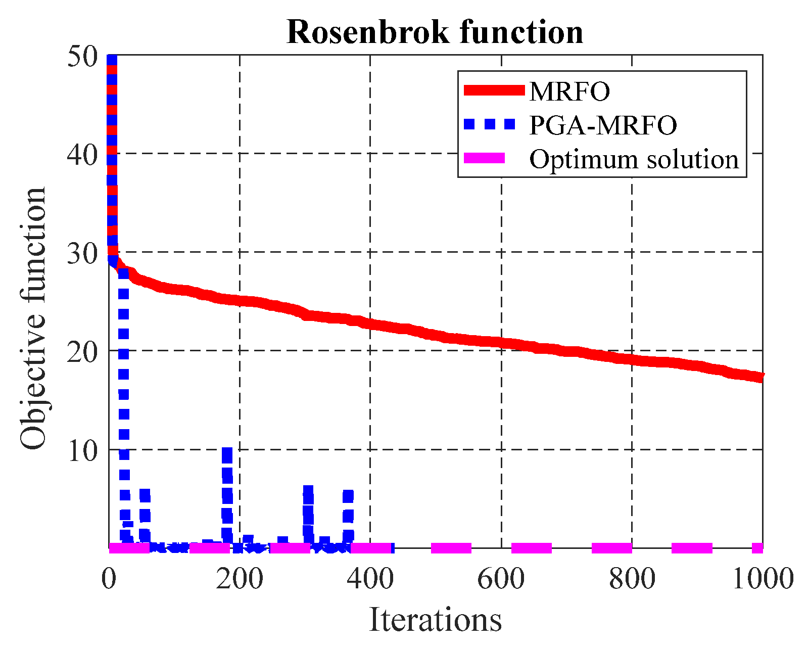
On the other hand, Figure 2, Figure 3, Figure 4, Figure 5, Figure 6, Figure 7, Figure 8, Figure 9, Figure 10 and Figure 11 show the converges curves to the optimum solution by the classical MRFO and the proposed PGA-MRFO algorithm for all test functions. From the table and figures, we can see that:

• For F₅ (Figure 2), the PGA-MRFO algorithm converges to the optimum solution in 438 iterations. But the MRFO algorithm consumed 1000 iterations and could not reach the optimum solution.
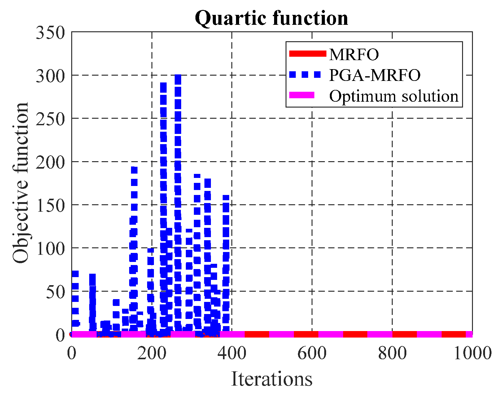
• For F₇ (Figure 3), the PGA-MRFO algorithm converges to the optimum solution in fewer iterations than the MRFO algorithm.
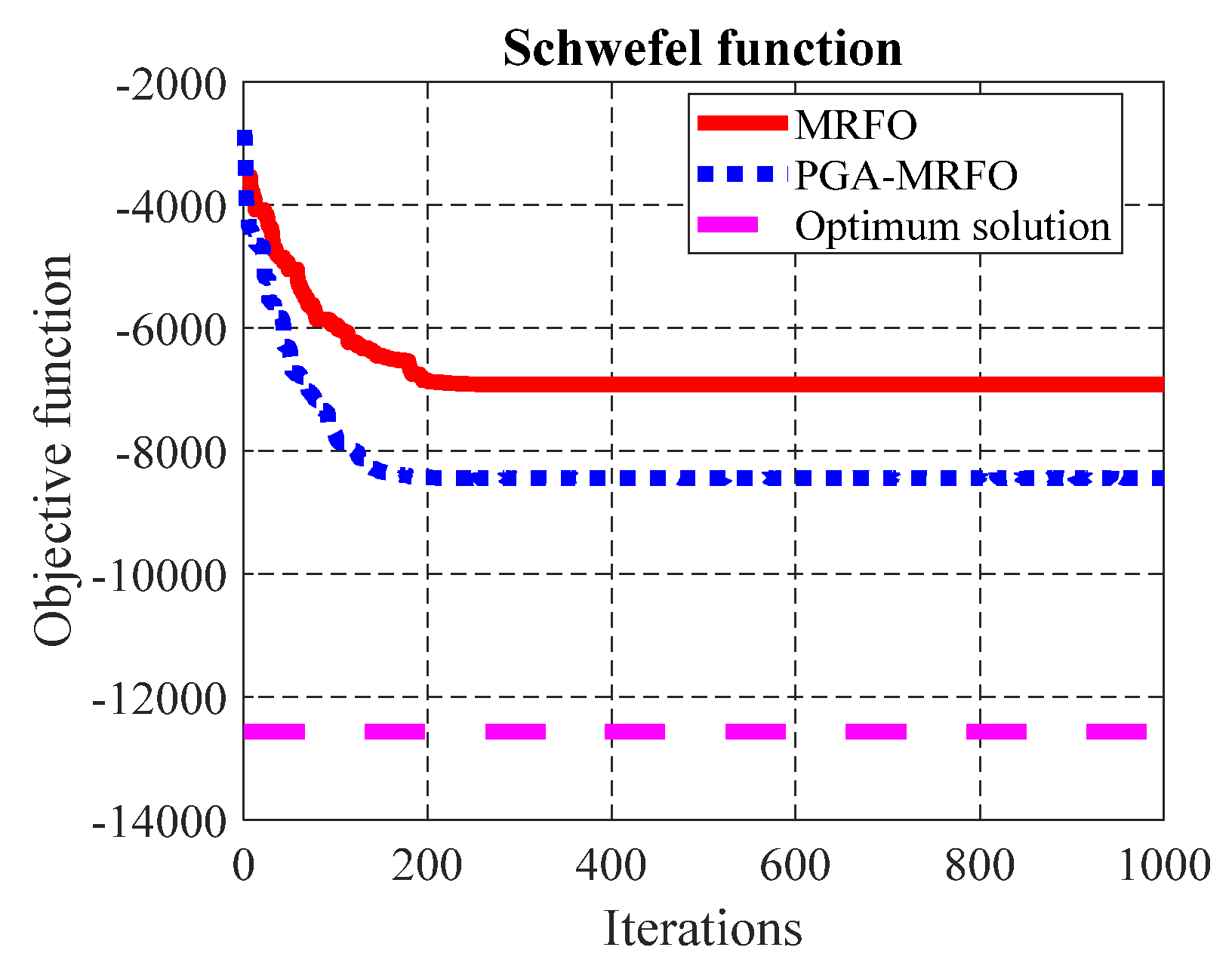
• For F₈ (Figure 4), both algorithms failed to reach the optimum solution during 1000 iterations. However, PGA-MRFO converged to a better solution than the MRFO algorithm in the same number of iterations.
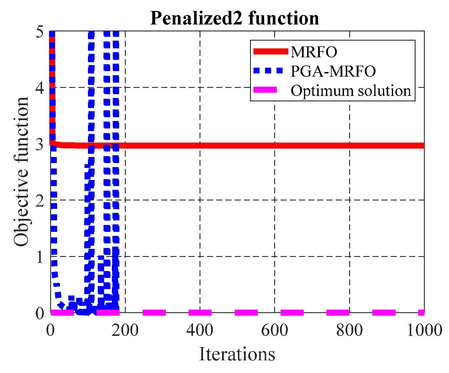
• For F₁₃ (Figure 5), the PGA-MRFO algorithm reached the optimum solution using 181 iterations. The MRFO algorithm consumed 1000 iterations and failed to converge to the optimum solution.
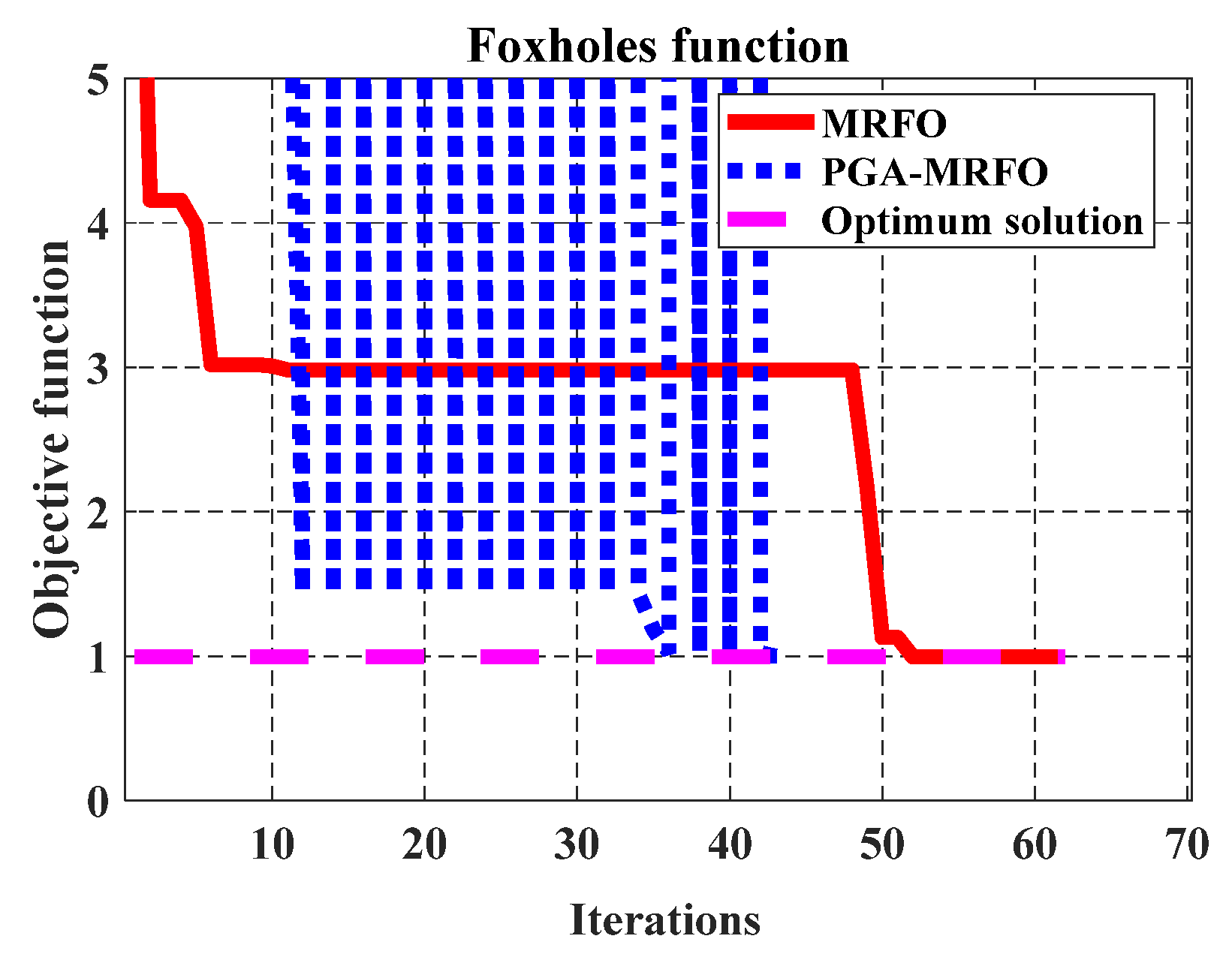
• For F₁₄ (Figure 6), the PGA-MRFO reached the optimum solution in fewer iterations than the MRFO algorithm. It should be noticed that the fluctuations in the results using the PGA-MRFO algorithm represent the trials of the algorithm to get out of the local minimum and move to a better solution.
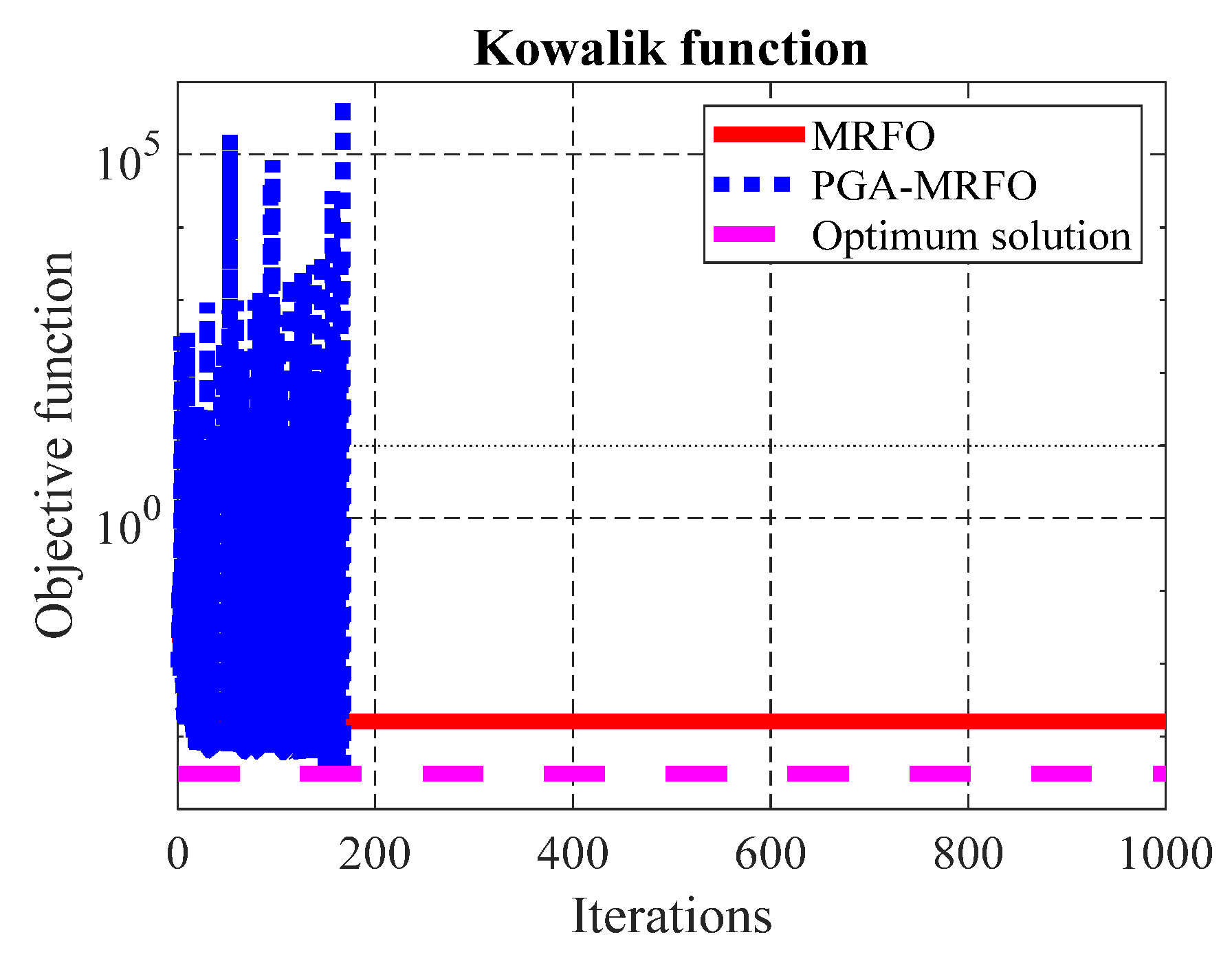
• For F₁₅ (Figure 7), the PGA-MRFO reached the optimum solution in 169 iterations, while the MRFO algorithm could not get a near-optimal solution even after using 1000 iterations.
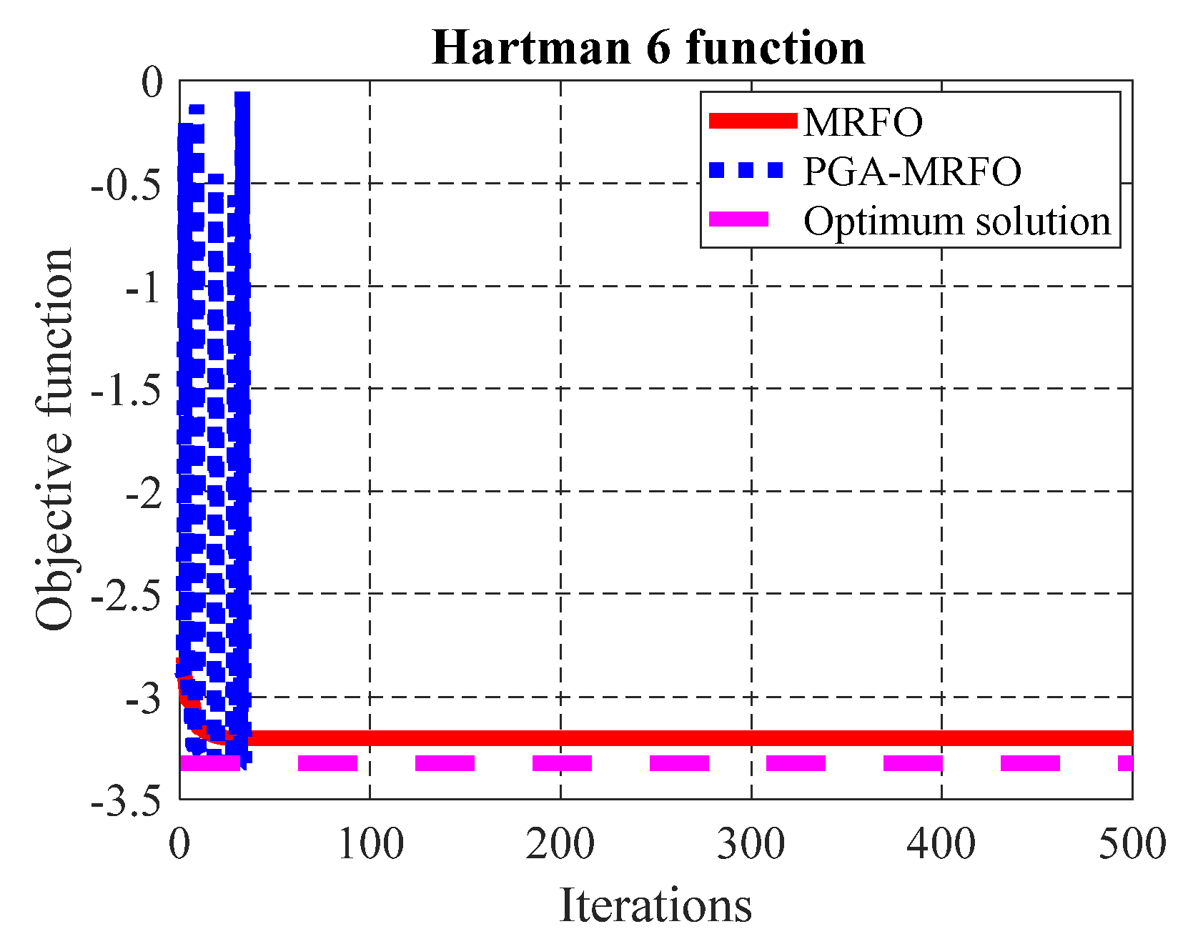
• For F₂₀ (Figure 8), the PGA-MRFO algorithm converges to the optimum solution in 35 iterations. But, the MRFO algorithm spent 500 iterations and could not reach the optimum solution due to trapping in the local minimum.
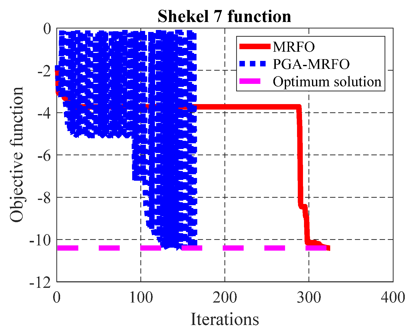
• For F₂₁ (Figure 9), the PGA-MRFO algorithm got the optimum solution in 109 iterations. The MRFO algorithm consumed 1000 iterations without converging to the optimum solution due to falling into the local minimum.
• For F₂₂ (Figure 10), the PGA-MRFO algorithm got the optimum solution in 169 iterations. But, the MRFO algorithm needed 325 iterations to reach the optimum solution, where this number of additional iterations was wasted in trapping into the local minimum.
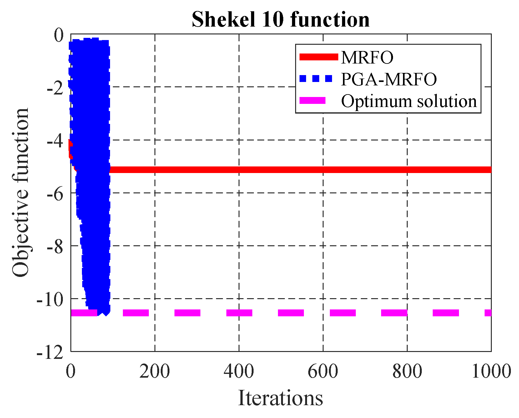
• For F₂₃ (Figure 11), the PGA-MRFO algorithm got the optimum solution in 87 iterations. In contrast, the MRFO algorithm spent 1000 iterations and could not converge to the optimum solution. The figure shows that the MRFO algorithm consumed more than 800 iterations with almost the same solution due to trapping into the local minimum. But, the PGA-MRFO algorithm fluctuated until getting out of the local minimum and reached the optimum solution.

To further clarify, both algorithms, classical MRFO and the PGA-MRFO, are applied to the 13 test functions with the possibility of increasing dimensions [17]. The dimensions of these problems are increased to 100. Besides, the GA is applied to the same functions for more illustration of the comparison. The maximum number of generations is 50, and the population size is 20 for the three algorithms to accelerate the calculations for this high dimension’s cases.

Table 2. Comparison between the three algorithms according to consumed iterations.

Test Function	Function	D	Domain	NO. of Iterations Using MRFO	NO. of Iterations Using GA	NO. of Iterations Using PGA-MRFO	Percentage Improvement between PGA-MRFO and
							MRFO	GA
Sphere	F1	100	$\left[-100, 100\right]$	50	50	7	86%	86%
Schwefel 2.22	F2	100	[−10, 10]	50	50	3	94%	94%
Schwefel 1.2	F3	100	$\left[-100, 100\right]$	50	50	5	90%	90%
Schwefel 2.21	F4	100	$[-100, 100$]	50	50	6	88%	88%
Rosenbrock	F5	100	$\left[-30, 30\right]$	50	50	4	92%	92%
Step	F6	100	[−100, 100]	50	50	5	90%	90%
Quartic	F7	100	$\left[-1.28, 1.28\right]$	50	50	22	56%	56%
Schwefel	F8	100	$\left[-500, 500\right]$	50	30	30	44%	0%
Rastrigin	F9	100	$\left[-5.12, 5.12\right]$	50	50	3	94%	94%
Ackley	F10	100	$\left[-32, 32\right]$	50	50	7	86%	86%
Griewank	F11	100	$\left[-600, 600\right]$	50	50	7	86%	86%
Penalized	F12	100	$\left[-50, 50\right]$	50	50	17	66%	66%
Penalized2	F13	100	$\left[-50, 50\right]$	50	50	10	80%	80%

illustrates the results of the three algorithms and the related percentage improvement according to Equation (32). As shown in the table, for high-dimensional problems, the suggested approach can reach the desired tolerance in fewer iterations.

5. Application of PGA-MRFO Algorithm to Unit Commitment Problem

5.1. Description of the Problem

Unit commitment (UC) problem is a nonlinear, mixed integer combinatorial optimization problem. The UC issue involves scheduling a power system generating units on or off mode over a given period to meet a specific objective. The UC is performed centrally by the utility control center based on a load forecast at a particular time. The aim is to minimize the total operation costs subject to different operating conditions. The operation costs include all generating units’ production and startup costs over the entire study time.

5.2. Problem Formulation

The UC problem can be formulated mathematically by presenting the objective function and the operating constraints. The objective function that represents the total operating cost of the system can be written as follows:

$$\underset{P_i, U_i}{\min }{\displaystyle \sum }_{k=1}^T{\displaystyle \sum }_{i=1}^N{U}_{i_k}·\left[F\left(P_{i_k}\right)+S_{i_k}\left(1-U_{i_{k-1}}\right)\right]$$

(33)

$$F\left(P_{i_k}\right)=\{ \begin{array}{c}{a}_i+b_i{P}_{i_k}+c_i{P}_{i_k}^2\\ or\\ F_{i0}+{\lambda }_i·H_i·P_{i_k}\end{array};$$

(34)

The following system constraints must be fulfilled:

• Power balance constraint:

The total generation must cover the whole load and system losses that can be neglected.

$${\displaystyle \sum }_{i=1}^{N_g}{U}_{i_k}·P_{i_k}=T_{1}L{D}_k$$

(35)

2.

Generation limits:

Generation units must be dispatched between the minimum and maximum limits of generation.

$$P_{i_k}^{min}\le P_{i_k}\le P_{i_k}^{max}$$

(36)

3.

Minimum up time:

The generation unit must be kept running for a specific time before turning it off, which can be formulated as follows:

$$U{T}_{i_k}=\left(U{T}_{i_{k-1}}+1\right)·u_{i_k}$$

(37)

$$\left(u_{i_{k-1}}-u_{i_k}\right)·U{T}_{i_{k-1}}\ge T_{i_{up-min}};$$

(38)

4.

Spinning reserve:

The total capacity of all generation units must cover the whole load and a specific reserve percentage. It can be formulated as follows:

$${\displaystyle \sum }_{i=1}^N{U}_{i_k}·P_{i_k}^{max}\ge TL{D}_k+R_k$$

(39)

5.3. Test System Cases

The proposed algorithm is applied to solve two cases of the UC problem.

5.3.1. Case 1: Four Units Test Power System

The data of the test system is given in

Table 3. Case 1—test system data.

	Unit 1	Unit 2	Unit 3	Unit 4
Pgmin [MW]	25	60	75	20
Pgmax [MW]	80	250	300	60
Inc. Heat rate [BTU/kWh]	10,440	9000	8730	11,900
Fuel cost [£/MBTU]	2	2	2	2
No load cost [£/h]	213	585.62	684.74	252
Min up time [h]	4	5	5	1
Min down time [h]	2	3	4	1
Startup cost [£]	150	170	500	0

. The load demand changes over eight intervals each of 3 h, as shown in Figure 12.

5.3.2. Case 2: Ten Units Test Power System

The data of the test system is given in

Table 4. Case 2—test system data.

	Unit 1	Unit 2	Unit 3	Unit 4	Unit 5	Unit 6	Unit 7	Unit 8	Unit 9	Unit 10
Pgmin [MW]	30	130	165	130	225	50	250	110	275	75
Pgmax [MW]	100	400	600	420	700	200	750	375	850	250
Inc. Heat rate [BTU/kWh]	9000	10,000	1100	1120	1800	340	520	60	60	60
Fuel cost [£/MBTU]	2	2	2	2	2	2	2	2	2	2
No load cost [£/h]	1000	970	700	680	450	370	480	660	665	670
Min up time [h]	5	3	2	1	4	2	3	1	4	2
Min down time [h]	4	2	4	3	5	2	4	3	3	1
Startup cost [£]	2050	1460	2100	1480	2100	1360	2300	1370	2200	1180

. The load demand changes over 8 intervals each of 3 h, as shown in Figure 13.

5.4. Modify the PGA-MRFO to Solve UC Problem

The data in this problem is discrete. As a result, the concept of a continuous pseudo parameter cannot be applied here. The new individual will vary between a countable set of values. In addition, there is no need to use the α parameter that was defined by Equation (22). Since there is no need to calculate an approximation of the Jacobian in this discrete problem, the number of parameters is decreased to two parameters instead of three, and the ($\Delta s$) parameter domain will be [0 1], and the parameter (δ) still have the same domain. The reason will be explained in the detailed steps of the modified part of the algorithm. The minimization problem will be solved using the GA is defined as:

$$\left\{\begin{array}{c}\underset{\delta \in \left(0,1\right) , \Delta s\in \left[0,1\right]}{\min }\left|f_{new}-\delta f\right| if f\ge 0\\ \underset{\delta \in \left(0,1\right) , \Delta s\in \left[0,1\right]}{\min }\left|f_{new}-\frac{f}{\delta }\right| if f<0\end{array}\right\}$$

(40)

The PGA-MRFO algorithm basic steps are applied as explained before, except for the part related to the updated individual. In the continuous case, $\Delta X$ was calculated according to Equation (23). While in the discrete case, it will be approximated according to the following steps.

• Let $X=\left[x_1 x_2 x_3\dots .x_n\right]$ be the best individual that is stuck in a local minimum.
• The limits of change in each variable [$x_i\in X$] can be calculated as:

  $$span\left(x_i\right)=\left[x_{ilow}-x_i, x_{iup}-x_i\right]$$

  (41)
• Each variable’s available set of discrete values represents the integer values between the lower and upper limits according to the span values calculated in step 1.

For example: Let $X=\left[3 2 0\right]$, and the lower and upper boundaries of the problem’s variables are $low=\left[0 1 0\right] and up=\left[5 7 4\right]$. According to Equation (40), the span of each variable in X is:

$$\{\begin{array}{c}span\left(x_1\right)=\left[-3 4\right]\\ span\left(x_2\right)=\left[-1 5\right]\\ span\left(x_3\right)=\left[0 4\right]\end{array}$$

(42)

Sequentially, the available set of cases for each variable (VC(i)) will be:

$$\{\begin{array}{c}VC\left(1\right)=\{-3,-2,-1,0,1,2,3,4]\}\\ VC\left(2\right)=\left\{-1,0,1,2,3,4,5\right\}\\ VC\left(3\right)=\left\{0,1,2,3,4\right\}\end{array}$$

(43)

4.

The two parameters in the GA are used to calculate the index of the proposed change in each variable. This index is approximated as:

$$\begin{gathered} dxindex\left(x_i\right)=Integer\left(\Delta s\ast lenght\left(VC\left(i\right)\right)\right) \\ dxindex=\left[dxindex\left(x_1\right) dxindex\left(x_2\right)\dots \dots \dots .dxindex\left(x_n\right)\right] \end{gathered}$$

(44)

Since the index cannot be less than one or more than the length of the set (VC(i)), the domain of the parameter (Δs) was replaced by [0 1], as mentioned before. Besides, if the (dxindex) is calculated as 0, it will be replaced by 1.

5.

After identifying the index, the new individual-based genetic parameters will be defined as:

$$d{x}_i=VC\left(dxindex\left(x_i\right)\right)$$

(45)

$$dx=\left[d{x}_1 d{x}_2\dots \dots .d{x}_n\right]$$

(46)

$$X_{new}=X+dx$$

(47)

For example: If $dxindex=\left(1, 3, 2\right)$, then $dx=\left[VC\left(1,1\right) VC\left(2,3\right) \left(3,2\right)\right]$. Finally, the new variable will be approximated as $X_{new}=\left[3 2 0\right]+\left[-3 1 1\right]=\left[0 3 1\right]$.

6.

For each individual in the genetic population, the new solution is calculated according to these five steps. Then, its objective function is calculated according to Equation (29), and the corresponding fitness function of the GA is calculated according to Equation (30).

These steps (from 1 to 6) replace steps 2 and 3 in the PGA-MRFO for the continuous domain problems. In addition, due to the modified domain of (Δs) parameter and the dispensing of Jacobian calculations, there is no need to apply the correction step indicated by Equation (28). The new variables will always be in the feasible region. As mentioned before, the rest of the algorithm is used until the stopping criterion is achieved. The dynamic programming (DP), the particle swarm optimization (PSO), the classical MRFO algorithm, and the PGA-MRFO algorithms will be applied to the application problem.

5.4.1. Results of UC Problem—Case 1

Table 5. Results of the four algorithms for the UC problem—Case 1 with a constant population size of 100.

Max. Generations = 100
Algorithm	DP	PSO	MRFO	PGA-MRFO
Total cost	74,110	75,006	74,643	73,274
Consumed iterations	-	100	100	6
Max. Generations = 300
Algorithm	DP	PSO	MRFO	PGA-MRFO
Total cost	74,110	75,006	73,559	73,274
Consumed iterations	-	300	300	7
Max. Generations = 500
Algorithm	DP	PSO	MRFO	PGA-MRFO
Total cost	74,110	75,006	74,027	73,274
Consumed iterations	-	500	500	10

shows the results of the four algorithms in the three different scenarios. The population consists of 100 individuals in all scenarios. But the maximum number of generations is 100 in scenario 1, 300 in scenario 2, and 500 in scenario 3. These numbers were chosen randomly to examine the performance of algorithms during a broader range of iterations. The optimum solution for this case is (73,274). As a result, it is used as the tolerance indicator. If any algorithm reaches this solution, it will terminate, and the consumed iterations’ number is recorded. Otherwise, the research process will continue until reaching the maximum number of generations. The DP algorithm does not depend on iterations as with other algorithms. So, its results will be included only in tables. In the three scenarios, the proposed algorithm discovers the optimum solution in a few iterations, whereas the other algorithms, DP, PSO, and standard MRFO, utilized all iterations and failed to locate the optimal solution, as shown in Table 5.

In addition, Figure 14, Figure 15 and Figure 16 show the converge curves to the optimum solution obtained by DP, PSO, the classical MRFO, and the proposed PGA-MRFO algorithm for all three scenarios. The proposed PGA-MRFO algorithm found the optimum solution in a very small number of iterations, as shown in the figures. While the other algorithms, PSO and MRFO, consumed the whole number of iterations without reaching the optimal solution, even when the population size grew larger.

5.4.2. Results of UC Problem—Case 2

The same procedures in case-1 are applied in this case. The four algorithms, DP, PSO, classical MRFO, and the proposed PGA-MRFO algorithm are used to solve this case.

Table 6. Results of the four algorithms for the UC problem—Case 2 with a constant population size of 100.

Max. Generations = 100
Algorithm	DP	PSO	MRFO	PGA-MRFO
Total cost	38,271	91,152	42,514	37,765
Max. Generations = 300
Algorithm	DP	PSO	MRFO	PGA-MRFO
Total cost	38,271	91,152	49,993	36,304
Max. Generations = 500
Algorithm	DP	PSO	MRFO	PGA-MRFO
Total cost	38,271	91,152	49,993	36,303

summarizes the results for this case at 100 population size and three scenarios of generations number (100, 300, 500). Since the UC-case 1’s optimum solution was known, it was employed as a tolerance for the termination criterion. In UC-case 2, however, it is unknown, hence all iterative algorithms are applied until the generation number ends. Then, the best solution is recorded. In each of the three scenarios, the PGA-MRFO method outperforms the DP, PSO, and standard MRFO algorithms and obtains the best solution. Finally, the results of this section illustrate the ability of the proposed algorithm to solve both continuous and discrete problems and its ability to overcome trapping into the local minimum and reach the optimum solution in fewer iterations.

6. Analysis of the Proposed Algorithm

Several analyses will be applied to the proposed algorithm in this section. These analyses aim to illustrate the effectiveness and reliability of the proposed algorithm. In addition, additional comparisons will be added to show the improvements suggested by the proposed algorithm.

6.1. Uncertainty Analysis of the Proposed Algorithm

Uncertainty analysis aims to quantify the variability of the output due to the variability of the input. The quantification is most often performed by estimating statistical measurements such as mean and standard deviation. The load disturbance and fuel cost in the UC problem are considered examples of uncertainty parameters in this research.

(1) Load disturbance: A total of 20 different cases of load disturbance were considered to clarify the effect of uncertainty on the calculations of the optimum solution. The load disturbances were randomly calculated by increasing or decreasing as a percentage of the original loads. The load uncertainty cases are taken from 1% to 20% of the original case. The population size is 20, and the maximum number of generations is 50 for the four algorithms, DP, PSO, MRFO, and PGA-MRFO, in all cases. These cases are applied to the model of the UC problem—Case 1 illustrated in the previous section.

Table 7. Algorithms’ results due to load uncertainty.

Algorithm	DP Optimum Cost	PSO Optimum Cost	MRFO Optimum Cost	PGA-MRFO Optimum Cost
Uncertainty Load Percentage
Original case (0%)	74,110	74,721	74,207	73,274
Original case ± 1%	74,070	73,961	74,589	74,059
Original case ± 2%	74,031	73,885	74,531	73,982
Original case ± 3%	75,020	74,246	74,524	74,344
Original case ± 4%	72,972	75,641	75,075	74,141
Original case ± 5%	75,176	74,054	73,190	72,256
Original case ± 6%	72,538	76,414	75,914	74,981
Original case ± 7%	75,766	74,583	73,968	73,034
Original case ± 8%	73,416	74,404	74,157	73,224
Original case ± 9%	76,778	75,441	75,742	74,865
Original case ± 10%	74,734	77,390	76,969	75,765
Original case ± 11%	73,902	75,001.9	74,865.9	74,065.1
Original case ± 12%	76,283	74,629	74,280	72,712
Original case ± 13%	76,290	77,857	77,406	76,253
Original case ± 14%	75,773	77,185	76,468	75,535
Original case ± 15%	74,099	76,839	77,237	75,842
Original case ± 16%	74,099	71,984	71,366	70,446
Original case ± 17%	77,743	80,247	79,536	78,603
Original case ± 18%	76,210	77,568	76,980	75,650
Original case ± 19%	71,211	69,903	69,195	67,618
Original case ± 20%	76,803	76,699	75,563	74,629
Mean	74,845.7	75,396.6	75,077.795	74,100.205
Standard deviation	2288.401536	2271.454	2247.9908	1641.46196

shows the best solution obtained from the four algorithms for the original load data and the uncertainty load data. Besides, it shows the mean and the standard deviation for the different instances of load uncertainty. The results illustrate uncertainty influence on the proposed algorithm compared to the other algorithms. The PGA-MRFO has the closest mean value to the original case than other algorithms despite the uncertainty percentage reaching 20%. In addition, the proposed algorithm standard deviation is less than other algorithms, which means the calculated solution in each case is almost close to that mean.

(2) Fuel cost: Since the fuel price changes continuously, it can be considered a source of uncertainty in the calculations of the UC problem. So, 20 cases of disturbance or uncertainty of fuel cost are considered. The uncertainty is considered from 1% to 20% of the original price indicated in the model of the UC problem—Case 1 illustrated in the previous section. The DP, PSO, MRFO, and PGA-MRFO results are recorded in

Table 8. Algorithms’ results due to fuel cost uncertainty.

Algorithm	DP Optimum Cost	PSO Optimum Cost	MRFO Optimum Cost	PGA-MRFO Optimum Cost
Uncertainty Fuel Cost Percentage
Original case (0%)	74,110	74,721	74,207	73,274
Original case ± 1%	73,866	74,499	73,989	73,051
Original case ± 2%	75,104	75,696	75,188	74,288
Original case ± 3%	73,672	74,423	73,944	72,974
Original case ± 4%	74,527	75,073	74,872	73,647
Original case ± 5%	74,080	74,601	74,343	73,074
Original case ± 6%	74,372	75,056	74,622	73,672
Original case ± 7%	72,515	73,216	72,688	71,659
Original case ± 8%	74,140	75,054	74,681	73,737
Original case ± 9%	75,986	76,919	76,621	76,323
Original case ± 10%	74,621	75,853	74,956	75,115
Original case ± 11%	74,907	75,572	75,069	74,113
Original case ± 12%	72,092	72,655	72,304	70,981
Original case ± 13%	72,012	73,304	73,099	72,724
Original case ± 14%	73,760	74,866	74,777	73,881
Original case ± 15%	81,207	81,960	81,648	80,780
Original case ± 16%	82,712	84,993	84,088	82,424
Original case ± 17%	74,027	76,146	74,147	72,636
Original case ± 18%	75,351	75,882	76,222	74,607
Original case ± 19%	77,183	80,019	78,332	77,228
Original case ± 20%	65,573	66,482	66,288	65,425
Mean	74,596.5	75,670.78	75,150.06	74,166.67
Standard deviation	3471.103	3686.144	3536.355	3408.60549

.

Table 8 illustrates that the suggested algorithm’s mean uncertainty cases are the closest to the problem’s results and solution when using the original data. In addition, the results show that the dispersion of results around the mean in the case of the proposed algorithm is better than the other algorithms. Finally, the tables and results clarify the effectiveness of the proposed algorithm in cases of uncertainty in the examined UC problem.

6.2. Robustness Analysis of the Proposed Algorithm

The algorithm robustness can be expressed as the ability of the algorithm to reach a good solution in most times that it is applied. Besides, the ability to provide good results in other problems of the same type can be another robustness analysis measure. The test functions have illustrated the proposed algorithm’s robustness versus various problems. However, the recurrence application of the proposed algorithm will be explored to verify its robustness from the first point of view. Three cases of operations and recurrence will be applied. First, the algorithm will be applied to constant population size and a different size of generations. Second, the maximum number of generations remains constant with varying the population size. Finally, it will be applied to one of the algorithm’s parameters. The UC problem—Case 1 will be used for these analyses.

(Robustness analysis case-1) The PGA-MRFO algorithm is applied with a constant population size (20) while the maximum generations number varies from 10 to 200. Figure 17 shows the results of this case in detail, where the resulting optimum solution variation is calculated by the PGA-MRFO algorithm versus the size of the generations.

(Robustness analysis case-2) In this case, The PGA-MRFO algorithm is applied with a constant number of generations (50) while the population size varies from 10 to 200. Figure 18 shows the relationship between the calculated optimum solution and population size.

(Robustness analysis case-3) The PGA-MRFO algorithm is a hybrid between the MRFO algorithm and the GA algorithm, so it is affected by their parameters. The MRFO algorithm depends on random parameters that vary continuously with individuals and during generations. The parameter $\left(r_1\right)$ is one of these parameters. The robustness of the proposed algorithm versus this parameter will be explored. $r_1$ was chosen for investigation since it is a common parameter in MRFO, whereas the other parameters differ depending on the number of system variables. 20 constant values between (0,1) of this parameter have been considered and tested by the proposed algorithm. In the basic algorithm, this parameter is changed each iteration randomly. So, in this examination, each value of $r_1$ will remain constant until the termination of the optimization process, and the resulting solution will be recorded. Figure 19 shows the variation of the optimum solution obtained from the proposed algorithm versus the parameter $r_1$.

Figure 17, Figure 18 and Figure 19 show how the PGA-MRFO algorithm often reaches the same solution versus different parameter values of $r_1$, indicating its robustness and reliability. The mean and standard deviation for each case will be calculated for further analysis. Besides, the percentage error between the mean and the original best solution will be calculated to evaluate the deviation of that mean from the optimum solution. While the optimum solution is considered as calculated in Section 4, which equals (73,274). This percentage will be calculated as:

$$Error=\frac{mean-optimum solution }{optimum solution}\times 100$$

(48)

Table 9. The statistical measures and error for robustness analysis.

Parameter	Mean	Standard Deviation	Error
Maximum number of Generations	73,447.75	367.4222	0.002371
Population size	73,373.55	408.031	0.001358
$\mathrm{Parameter} r_1$	73,377.1	329.5517	0.001407

shows the mean and standard deviation values of each case of robustness examination mentioned before. The table illustrates that, despite different changes in the corresponding parameters, the PGA-MRFO algorithm could detect the optimum or near optimum solution with minimum error, showing its robustness and availability.

6.3. Time Complexity and Computational Time Analysis of PGA-MRFO

In the following, three strategies are introduced to analyze the time complexity and computational time of PGA-MRFO:

• The time complexity may be considered the amount of time an algorithm takes to be executed as a function of the input size. Here, the input size indicates the number of operations performed by the algorithm. The PGA-MRFO algorithm’s time complexity may be considered the result of the classical MRFO’s time complexity and the genetic algorithm’s time complexity. The genetic algorithm’s time complexity is considered as $O\left(DGP\right)$ Where; D is the problem dimension, G is the maximum number of generations, and P is the population size. While in the proposed algorithm, the dimension in the genetic loop is constant (3), its time complexity reduces to be $O\left(3GP\right)$ or after approximation $O\left(GP\right)$. So, the time complexity of the PGA-MRFO algorithm is less than that of the hybridization algorithm between GA and classical MRFO.
• The actual computation time of the PGA-MRFO algorithm is calculated through different cases of a problem. Then, curve fitting is used to identify this time as a function of specific parameters. In this strategy, the parameters will be the dimensions of the problem and the maximum value between generations and population size. Since the time complexity depends on the problem dimensions and other parameters, it is essential to raise the dimensional easily to facilitate the investigation, which will not always be available in the UC problem. So, the time complexity analysis of the proposed algorithm will be discussed for the following test function:

$$F={\displaystyle \sum }_{i=1}^N{x}_i^2, x_i\in \left[-100,100\right]$$

(49)

The number of variables takes values from 10 to 500 will be considered the first parameter for fitting time complexity. While both generations and population size are created randomly between the range [10,200]. The maximum value between generations and population size will be considered the second parameter. The PGA-MRFO is applied for 50 cases within the determined range of generations and population size, and the time in minutes is recorded. The fitting toolbox in MATLAB is used to identify the best fitting surface for the available data to deduce an approximated formula of the computations time. So, The 5th-degree polynomial is selected. The resulted equation for approximation of time is the following equation:

$$\begin{array}{ll}\mathit{Approximated}& \mathit{time}\\ & =p_{00}+p_{10}x+p_{01}y+p_{20}{x}^2+p_{11}xy+p_{02}{y}^2+p_{30}x+p_{21}{x}^{2}y+p_{12}x{y}^2+p_{03}{y}^3\\ & +p_{40}{x}^4+p_{31}{x}^{3}y+p_{22}{x}^2{y}^2+p_{13}x{y}^3+p_{04}{y}^4+p_{50}{x}^5+p_{41}{x}^{4}y+p_{32}{x}^3{y}^2+p_{23}{x}^2{y}^3\\ & +p_{14}x{y}^4+p_{05}{y}^{5}xd\end{array}$$

(50)

The values of the approximated coefficients are shown in

Table 10. The values of the approximated coefficients.

Coefficient	${\mathit{p}}_{\mathbf{00}}$	${\mathit{p}}_{\mathbf{10}}$	${\mathit{p}}_{\mathbf{01}}$	${\mathit{p}}_{\mathbf{20}}$	${\mathit{p}}_{\mathbf{11}}$	${\mathit{p}}_{\mathbf{02}}$	${\mathit{p}}_{\mathbf{30}}$
Value	2.292	0.3527	1.301	−0.3958	−0.5647	−0.7977	0.1382
Coefficient	${\mathit{p}}_{\mathbf{21}}$	${\mathit{p}}_{\mathbf{12}}$	${\mathit{p}}_{\mathbf{03}}$	${\mathit{p}}_{\mathbf{40}}$	${\mathit{p}}_{\mathbf{31}}$	${\mathit{p}}_{\mathbf{22}}$	${\mathit{p}}_{\mathbf{13}}$
Value	−1.22	0.466	−0.5679	0.2399	−0.3286	−0.06093	0.8375
Coefficient	${\mathit{p}}_{\mathbf{04}}$	${\mathit{p}}_{\mathbf{50}}$	${\mathit{p}}_{\mathbf{41}}$	${\mathit{p}}_{\mathbf{32}}$	${\mathit{p}}_{\mathbf{23}}$	${\mathit{p}}_{\mathbf{14}}$	${\mathit{p}}_{\mathbf{05}}$
Value	0.670	0.07944	0.03898	−0.2443	0.4315	0.16	0.3069

. While the surface of fitting the calculations time versus the dimensions and the maximum value between population size and generations is shown in Figure 20.

Indeed, other variables, such as algorithm parameters and the objective function’s computation time, affect the computation time. The latter depends on the objective function and its equations and not only on the dimensions of the problem. More analysis of the time complexity of the proposed algorithm can be investigated in future work.

• Another strategy to illustrate the improvement resulting from the proposed PGA-MRFO algorithm is to apply it and the MRFO algorithm to the objective function of Equation (49). The problem dimension varies from 10 to 500, yielding 50 cases, while the maximum generations and population size will be fixed at (100, 50). Figure 21 shows the comparison between PGA-MRFO and MRFO calculation time.

Figure 21 shows, in most cases, that despite the proposed algorithm combining two algorithms, it reaches the desired tolerance faster than the original MRFO, especially for high dimensions. We can say that the proposed algorithm saves time that may be wasted by the MRFO when it is stuck in a local minimum. So, from that point of view, PGA-MRFO is considered to have fewer computations time and consequently less burden than the original MRFO. In addition,

Table 11. The mean and standard deviations of the calculated time for algorithms based on 50 cases.

Algorithm	MRFO	PGA-MRFO
Mean value	0.050418	0.043794
Standard deviation	0.02474438	0.021480797

shows the mean value and standard deviation of the calculated time for both algorithms based on the 50 cases mentioned before.

In most test cases, the proposed algorithm takes less time, as shown in Table 11. Although the MRFO takes less time than the PGA-MRFO in some cases, the proposed algorithm’s meantime is less than that of the MRFO. Finally, tables and figures demonstrate the applicability and benefits of the proposed algorithm.

7. Conclusions

This paper introduced a hybrid optimization algorithm based on the classical MRFO and pseudo genetic algorithms. The proposed algorithm aims to solve the MRFO algorithm falling into the local minima, which consumes iterations without improvement. The PGA is the Genetic algorithm-based pseudo parameter to reduce the number of variables in the GA algorithm. A sub-optimization problem was derived based on the pseudo parameter and optimality condition. After solving the sub-problem, the best solution is updated, and the MRFO passes the local minimum. MRFO has applied again until it falls into another local minimum. The search is continued until the termination criterion is reached. The PGA-MRFO was applied to the test functions stuck in the local minimum in the original MRFO paper [17]. The results show how the proposed hybridization enhanced the performance of the MRFO algorithm and enabled it to reach the optimum solution. In addition, the algorithm was applied to the 13 test functions in [17], so that their dimensions can be increased. Besides, it was applied to the unit commitment (UC) problem to illustrate its validity and efficiency. Some modifications were added to the PGA-MRFO algorithm to fit this type of problem. The results of the PGA-MRFO algorithm were compared to the DP, PSO, and the classical MRFO algorithms. Uncertainty, robustness, and time analysis were investigated for the proposed algorithm to illustrate its properties. All of the results show that the proposed algorithm is superior to other algorithms in terms of reaching the optimal solution in a few iterations, whether the population size changes or the maximum number of generations.

In our future work, three directions will be prioritized: (i) Adding further PGA-MRFO adjustments and evaluating their impact on optimization results. (ii) PGA-MRFO can be used to tackle optimization problems in various fields. (iii) Use PGA-MRFO to improve existing metaheuristic algorithms, such as the moth search (MS) algorithm, the slime mould algorithm (SMA), the hunger games search (HGS), the Runge Kutta optimizer (RUN), the colony predation algorithm, and the Harris hawk’s optimization (HHO).

References

1. Michael, B.-B. Nonlinear Optimization with Engineering Applications. In Springer Optimization and Its Applications; Springer: Berlin/Heidelberg, Germany, 2008. [Google Scholar]
2. Rao, S.S. Engineering Optimization: Theory and Practice, 3rd ed.; Wiley: Hoboken, NY, USA, 2009. [Google Scholar]
3. Michalewicz, Z. Evolutionary Computation Techniques for Nonlinear Programming Problems. Int. Trans. Oper. Res. 2008, 1, 223–240. [Google Scholar] [CrossRef] [Green Version]
4. Onwubolu, G.C.; Babu, B.V. New Optimization Techniques in Engineering; Springer Science & Business Media: Berlin/Heidelberg, Germany, 2004; Volume 141. [Google Scholar]
5. John, H.H. Genetic Algorithms. Sci. Am. 1992, 267, 66–73. [Google Scholar]
6. Sastry, K.; Goldberg, D.; Kendall, G. Genetic Algorithms. In Search Methodologies; Burke, E.K., Kendall, G., Eds.; Springer: Boston, MA, USA, 2005. [Google Scholar]
7. El-Desoky, I.M.; El-Shorbagy, M.A.; Nasr, S.M.; Hendawy, Z.M.; Mousa, A.A. A hybrid genetic algorithm for job shop scheduling problems. Int. J. Adv. Eng. Technol. Comput. Sci. 2016, 1, 6–17. [Google Scholar]
8. El-Shorbagy, A.M.; Ayoub, A.Y.; El-Desoky, I.M.; Mousa, A.A. A Novel Genetic Algorithm Based K-Means Algorithm for Cluster Analysis. In International Conference on Advanced Machine Learning Technologies and Applications; Springer: Cham, Switherland, 2018; pp. 92–101. [Google Scholar]
9. Storn, R.; Price, K. Differential evolution-a simple and efficient heuristic for global optimization over continuous spaces. J. Glob. Optim. 1997, 11, 341–359. [Google Scholar] [CrossRef]
10. Simon, D. Evolutionary Optimization Algorithms; John Wiley & Sons, Ltd.: Hoboken, NJ, USA, 2013. [Google Scholar]
11. Beni, G.; Wang, J. Swarm Intelligence in Cellular Robotic Systems. In Proceedings of the NATO Advanced Workshop on Robots and Biological Systems, Tuscany, Italy, 26–30 June 1989; Springer: Berlin/Heidelberg, Germany, 1989; pp. 703–712. [Google Scholar]
12. El-Shorbagy, M.; Hassanien, A.E. Particle swarm optimization from theory to applications. Int. J. Rough Sets Data Anal. 2018, 5, 1–24. [Google Scholar] [CrossRef]
13. El-Shorbagy, M.A.; El-Shorbagy, M. Weighted Method Based Trust Region-Particle Swarm Optimization for Multi-Objective Optimization. Am. J. Appl. Math. 2015, 3, 81. [Google Scholar] [CrossRef]
14. Allah, A.M.A.; El-Shorbagy, M.A. Enhanced Particle Swarm Optimization Based Local Search for Reactive Power Compensation Problem; Scientific Research Publishing: Wuhan, China, 2012. [Google Scholar]
15. Dorigo, M.; Stutzle, T. Ant Colony Optimization; MIT Press: Cambridge, MA, USA, 2004. [Google Scholar]
16. Saremi, S.; Mirjalili, S.; Lewis, A. Grasshopper Optimisation Algorithm: Theory and application. Adv. Eng. Softw. 2017, 105, 30–47. [Google Scholar] [CrossRef] [Green Version]
17. Zhao, W.; Zhang, Z.; Wang, L. Manta ray foraging optimization: An effective bio-inspired optimizer for engineering applications. Eng. Appl. Artif. Intell. 2020, 87, 103300. [Google Scholar] [CrossRef]
18. Zhang, Y.; Jin, Z. Group teaching optimization algorithm: A novel metaheuristic method for solving global optimization problems. Expert Syst. Appl. 2020, 148, 113246. [Google Scholar] [CrossRef]
19. Atashpaz-Gargari, E.; Lucas, C. Imperialist competitive algorithm: An algorithm for optimization inspired by imperialistic competition. In Proceedings of the 2007 IEEE Congress on Evolutionary Computation, Singapore, 25–28 September 2007; pp. 4661–4667. [Google Scholar]
20. Rao, R.; Savsani, V.; Vakharia, D. Teaching–Learning-Based Optimization: An optimization method for continuous non-linear large scale problems. Inf. Sci. 2012, 183, 1–15. [Google Scholar] [CrossRef]
21. Kashan, A.H. An efficient algorithm for constrained global optimization and application to mechanical engineering design: League championship algorithm (LCA). Comput. Des. 2011, 43, 1769–1792. [Google Scholar]
22. Askari, Q.; Younas, I.; Saeed, M. Political Optimizer: A novel socio-inspired meta-heuristic for global optimization. Knowl.-Based Syst. 2020, 195, 105709. [Google Scholar] [CrossRef]
23. Rashedi, E.; Nezamabadi-Pour, H.; Saryazdi, S. GSA: A Gravitational Search Algorithm. Inf. Sci. 2009, 179, 2232–2248. [Google Scholar] [CrossRef]
24. Tayarani-N, M.H.; Akbarzadeh-T, M.R. Magnetic Optimization Algorithms a New Synthesis. In Proceedings of the2008 IEEE Congress on Evolutionary Computation (IEEE World Congress on Computational Intelligence), Hong Kong, China, 1–6 June 2008; pp. 2659–2664. [Google Scholar]
25. Van Laarhoven, P.J.M.; Aarts, E.H.L. Simulated Annealing. In Simulated Annealing: Theory and Applications; Springer: Dordrecht, The Netherlands, 1978; pp. 7–15. [Google Scholar]
26. Izci, D.; Ekinci, S.; Eker, E.; Kayri, M. Improved manta ray foraging optimization using opposition-based learning for optimization problems. In Proceedings of the 2020 International Congress on Human-Computer Interaction Optimization and Robotic Applications (HORA), Ankara, Turkey, 26–27 June 2020; pp. 1–6. [Google Scholar]
27. Mohamed; Hassan, H.; Essam; Houssein, H.; Mohamed; Mahdy, A.; Kamel, S. An improved Manta ray foraging optimizer for cost-effective emission dispatch problems. Eng. Appl. Artif. Intell. 2021, 100, 1–20. [Google Scholar]
28. Muralikrishnan, N.; Jebaraj, L.; Rajan, C.C.A. A Comprehensive Review on Evolutionary Optimization Techniques Applied for Unit Commitment Problem. IEEE Access 2020, 8, 132980–133014. [Google Scholar] [CrossRef]
29. Shadaksharappa, N.M. Optimum Generation Scheduling for Thermal Power Plants using Artificial Neural Network. Int. J. Electr. Comput. Eng. 2011, 1, 134–139. [Google Scholar] [CrossRef]
30. Dudek, G. Adaptive simulated annealing schedule to the unit commitment problem. Electr. Power Syst. Res. 2010, 80, 465–472. [Google Scholar] [CrossRef]
31. Sakthi, S.S.; Santhi, R.; Krishnan, N.M.; Ganesan, S.; Subramanian, S. Wind Integrated Thermal Unit Commitment Solution Using Grey Wolf Optimizer. Int. J. Electr. Comput. Eng. 2017, 7, 2309. [Google Scholar] [CrossRef]
32. Ponciroli, R.; Stauff, N.E.; Ramsey, J.; Ganda, F.; Vilim, R.B. An Improved Genetic Algorithm Approach to the Unit Commitment/Economic Dispatch Problem. IEEE Trans. Power Syst. 2020, 35, 4005–4013. [Google Scholar] [CrossRef]
33. Zhai, Y.; Liao, X.; Mu, N.; Le, J. A two-layer algorithm based on PSO for solving unit commitment problem. Soft Comput. 2020, 24, 9161–9178. [Google Scholar] [CrossRef]
34. Kamboj, V.K. A novel hybrid PSO–GWO approach for unit commitment problem. Neural Comput. Appl. 2016, 27, 1643–1655. [Google Scholar] [CrossRef]
35. Khunkitti, S.; Watson, N.R.; Chatthaworn, R.; Premrudeepreechacharn, S.; Siritaratiwat, A. An Improved DA-PSO Optimization Approach for Unit Commitment Problem. Energies 2019, 12, 2335. [Google Scholar] [CrossRef] [Green Version]
Figure 1. Flow chart of the proposed algorithm.
Mathematics 10 02179 g001
Figure 2. Converges curves for F5.
Mathematics 10 02179 g002
Figure 3. Converges curves for F7.
Mathematics 10 02179 g003
Figure 4. Converges curves for F8.
Mathematics 10 02179 g004
Figure 5. Converges curves for F13.
Mathematics 10 02179 g005
Figure 6. Converges curves for F14.
Mathematics 10 02179 g006
Figure 7. Converges curves for F15.
Mathematics 10 02179 g007
Figure 8. Converges curves for F20.
Mathematics 10 02179 g008
Figure 9. Converges curves for F21.
Mathematics 10 02179 g009
Figure 10. Converges curves for F22.
Mathematics 10 02179 g010
Figure 11. Converges curves for F23.
Mathematics 10 02179 g011
Figure 12. Load curve for case 1—test system.
Mathematics 10 02179 g012
Figure 13. Load curve for case 2—test system.
Mathematics 10 02179 g013
Figure 14. Converges curves for UC problem—Case 1 at max. Generations = 100.
Mathematics 10 02179 g014
Figure 15. Converges curves for UC problem—Case 1 at max. Generations = 300.
Mathematics 10 02179 g015
Figure 16. Converges curves for UC problem—Case 1 at max. Generations = 500.
Mathematics 10 02179 g016
Figure 17. Variation of the optimum solution versus the maximum number of generations.
Mathematics 10 02179 g017
Figure 18. Variation of the optimum solution versus population size.
Mathematics 10 02179 g018
Figure 19. Variation of the optimum solution versus the parameter ( r 1 ) .
Mathematics 10 02179 g019
Figure 20. The surface of fitting the calculations time.
Mathematics 10 02179 g020
Figure 21. Calculations time of MRFO and PGA-MRFO.
Mathematics 10 02179 g021