Fast Computation of Optimal Damping Parameters for Linear Vibrational Systems

Abstract

We propose a fast algorithm for computing optimal viscosities of dampers of a linear vibrational system. We are using a standard approach where the vibrational system is first modeled using the second-order structure. This structure yields a quadratic eigenvalue problem which is then linearized. Optimal viscosities are those for which the trace of the solution of the Lyapunov equation with the linearized matrix is minimal. Here, the free term of the Lyapunov equation is a low-rank matrix that depends on the eigenfrequencies that need to be damped. The optimization process in the standard approach requires $O\left(n^3\right)$ floating-point operations. In our approach, we transform the linearized matrix into an eigenvalue problem of a diagonal-plus-low-rank matrix whose eigenvectors have a Cauchy-like structure. Our algorithm is based on a new fast eigensolver for complex symmetric diagonal-plus-rank-one matrices and fast multiplication of linked Cauchy-like matrices, yielding computation of optimal viscosities for each choice of external dampers in $O\left(k{n}^2\right)$ operations, k being the number of dampers. The accuracy of our algorithm is compatible with the accuracy of the standard approach.

1. Introduction

We consider the determination of optimal damping for the vibrating structure which is represented by a linear vibrational system described by

$$M\ddot{x}+D\dot{x}+Kx=0,$$

(1)

where M and K (called mass and stiffness, respectively) are real, symmetric positive definite matrices of order n. The damping matrix is defined as

$$D=D_{int}+D_{ext},$$

(2)

where matrices $D_{int}$ and $D_{ext}$ correspond to internal and external damping, respectively. Internal damping can be modelled as

$$D_{int}=\alpha M^{1/2}\sqrt{M^{-1/2}K{M}^{-1/2}}{M}^{1/2},\alpha \in (0.005,0.1),$$

(3)

or

$$D_{int}=\alpha M+\beta K,\alpha ,\beta \in (0.005,0.1).$$

(4)

In Equation (3), we assume that the internal damping is a small multiple of the critical damping, while (4) corresponds to the so-called Rayleigh damping. Both cases are important and widely used in literature (see, e.g., books [1,2] or papers [3,4,5]) and they are interesting from a modeling point of view since the matrix that simultaneously diagonalizes matrices M and K, diagonalizes the internal damping matrix as well. In the Section 2.1 we give formulas for internal damping matrices in the modal coordinates. Moreover, analysis of the influence of different internal damping matrices is given in [6].

From the optimization point of view, we are more interested in the external viscous damping which can be modeled as

$$D_{ext}={\rho }_1{D}_1+{\rho }_2{D}_2+\cdots +{\rho }_k{D}_k,$$

(5)

where ${\rho }_i$ is the viscosity and $D_i$ describes a geometry of the corresponding damping position for $i=1,\dots ,k$. Throughout this paper, we will refer to the pair $({\rho }_i,D_i)$ as a damper. Typically, the system has very few dampers compared to the full dimension [1,2,7], which means that $k\ll n$. This is also the standard assumption all works from [3,4,8,9], where more details on the structure of internal and external damping can be found. For the full derivation of the problem and the solution and modeling procedure, we refer the reader to [2]. The model of linear vibrational system (1) corresponds to the quadratic eigenvalue problem

$$({\lambda }^{2}M+\lambda D+K)x=0,x\ne 0.$$

(6)

The damping optimization problem, in general, can be stated as follows: determine the “best” damping matrix D which insures optimal evanescence of each component of x. In practice, one can usually influence only the external damping. Therefore, the problem is to determine the optimal external damping matrix $D_{ext}$, which minimizes the total average energy of the system.

In order to optimize the external damping matrix from (5), we need to optimize the damping viscosities $({\rho }_1,\dots ,{\rho }_k)$ and the damping positions $D_1,\dots ,D_k$ such that the chosen optimization criterion is minimal. There exists several optimization criteria for this problem. One criterion is the so-called spectral abscissa criterion. This criterion requires that the maximal real part of the eigenvalues of the quadratic eigenvalue problem (6) are minimized (see, e.g., [10,11]).

In this paper, we will use a criterion based on the total average energy of the considered system. Detailed overview of the optimization criteria can be found in [2,12]. This criterion considers minimization of the total energy of the system (as a sum of kinetic and potential energy) averaged over all initial states of the unit total energy and a given frequency range. This criterion is equivalent to finding viscosities for which the trace of the solution of a certain Lyapunov equation involving the linearization of the quadratic eigenvalue problem (6) is minimal. Details about this linearization and the construction of the Lyapunov equation are given in Section 2.1. This criterion has many benefits and it was investigated widely in the last two decades. More details can be found, e.g., in [3,5,8,9,13,14,15]. Moreover, this criterion can be extended to the case where we consider Multiple-Input Multiple-Output systems that appear in the control theory in many applications, e.g., in paper [16] authors consider mixed control performance measure that includes also the total average energy into account.

In practice we optimize the geometry of considered vibrating structures such as n-mass oscillators or shear frame vibrating structures, for more details see, e.g., [2,6,8,11,17]. However, since the optimization of damping positions is a very hard problem, in this work we will concentrate only on the optimization of viscosities. This can be then applied for different damping positions or it can be used within the algorithm that optimizes damping positions, but we also emphasize that such algorithms are typically heuristic algorithms, see, e.g., [15]. Moreover, the objective function (which is in our case the total average energy) that needs to be minimized is a non-convex function that includes viscosity parameters and damping positions. Therefore, minimization of such objective function requires the evaluation of objective function a large number of times. Thus, directly applying the standard method requires $O\left(n^3\right)$ operations for each run, irrespective of the number of dampers. For the case of a small number of dampers k, which is typical in applications [2,7], we propose a fast method that requires $k{n}^2$ operations for each run.

In this paper, matrices are denoted by uppercase Greek or Roman letters, vectors are denoted by lowercase Roman letters, and scalars are denoted by lowercase Greek letters. As in Matlab, function $\mathrm{diag}$ is used twofold: when A is a matrix, $\mathrm{diag}\left(A\right)$ denotes the vectors of A’s diagonal elements. When $a={\left[\begin{array}{ccc}{a}_1& \cdots & a_n\end{array}\right]}^T$ is a vector, $\mathrm{diag}\left(a\right)$ and $\mathrm{diag}(a_1,\dots ,a_n)$ denote the square diagonal matrix with elements of a on its diagonal.

This paper is organized as follows: in Section 2 we describe the standard approach which uses linearization and minimizes trace of the solution of the respective Lyapunov equation. An overview of the existing $O\left(n^3\right)$ solution methods is presented in Section 2.1. A new approach, which uses complex symmetric linearization and reduces the problem to a sequence of k eigenvalue problems of complex symmetric diagonal-plus-rank-one (CSymDPR1) matrices, is presented in Section 2.2. Here, k is the number of dampers from (5). This approach uses fast multiplication of linked Cauchy-like matrices and needs $O\left(k{n}^2\right)$ operations in each optimization step. This makes the optimization using the new approach an order of magnitude faster than the standard approach if the number of dampers is small, $k\ll n$. Several large examples and some timings are given in Section 3. Discussion of our results and algorithms is presented in Section 4 and the conclusions are given in Section 5.

2. Methods

In this section, we describe solution methods for finding the optimal damping of the linear vibrational system (1) based on minimization of total average energy. First, we describe a linearization of the system (1), which yields a linearization of the quadratic eigenvalue problem (6). The linearization is performed by changing the basis and the linearized problem is further reduced to an eigenvalue problem of a simpler matrix. Of course, the corresponding quadratic eigenvalue problem can be solved by maintaining the second-order structure [18,19]. Although such approaches result in methods that works with matrices of dimension n instead of our approach that uses matrices of dimension $2n$, they still require $O\left(n^3\right)$ operations in each optimization step and can have numerical issues in some cases. Further, the linearization of the system is necessary for efficient calculation of total average energy [2,12].

In Section 2.1, we present an existing direct approach (see, e.g., [2,4]), where each iteration of optimization requires $O\left(n^3\right)$ operations. In Section 2.2, we describe the novel fast method which requires $O\left(k{n}^2\right)$ operations in each optimization step, thus outperforming the standard method in the case of a small number of dampers.

For a structured system, the problem (1) was considered in [8,9] where the authors proposed dimension reduction to accelerate the optimization process. However, to be efficient, dimension reduction requires a specific structure, so this approach cannot be applied efficiently in a general setting.

By symmetric linearization we transform quadratic eigenvalue problem (6) to the generalized eigenvalue problem (GEVP) (see, e.g., [20])

$$\left[\begin{array}{cc}0& K\\ K& D\end{array}\right]\left[\begin{array}{c}y\\ x\end{array}\right]=\lambda \left[\begin{array}{cc}K& 0\\ 0& -M\end{array}\right]\left[\begin{array}{c}y\\ x\end{array}\right].$$

(7)

Let

$${\mathsf{\Phi }}^{T}K\mathsf{\Phi }={\mathsf{\Omega }}^2,{\mathsf{\Phi }}^{T}M\mathsf{\Phi }=I.$$

(8)

be the generalized eigenvalue decomposition of the pair $(K,M)$. Since the calculation of matrices $\mathsf{\Phi }$ and $\mathsf{\Omega }$ does not depend on the damping matrix D, they can be calculated prior to the optimization procedure.

Both choices of $D_{int}$, from (3) and from (4) imply that $D_{int}$ is diagonal in the $\mathsf{\Phi }$-basis. More precisely,

$${\mathsf{\Phi }}^T{D}_{int}\mathsf{\Phi }\equiv \mathsf{\Gamma }=\alpha \mathsf{\Omega },$$

(9)

if $D_{int}$ is defined by (3), and

$${\mathsf{\Phi }}^T{D}_{int}\mathsf{\Phi }\equiv \mathsf{\Gamma }=\alpha I+\beta {\mathsf{\Omega }}^2,$$

(10)

if $D_{int}$ is defined by (4).

The external damping matrix, $D_{ext}$, is a low-rank matrix of rank k which depends on the number, positions, and the structure of dampers. For example, if all dampers are grounded and l is a vector of indices of damping positions, then $D_{ext}$ is zero except for ${\left[D_{ext}\right]}_{l\left[i\right],l\left[i\right]}=1$.

In the basis

$$\left[\begin{array}{cc}\mathsf{\Phi }& 0\\ 0& \mathsf{\Phi }\end{array}\right],$$

problem (7) reduces to GEVP

$$\left[\begin{array}{cc}0& {\mathsf{\Omega }}^2\\ {\mathsf{\Omega }}^2& \mathsf{\Gamma }+{\mathsf{\Phi }}^T{D}_{ext}\mathsf{\Phi }\end{array}\right]x=\lambda \left[\begin{array}{cc}{\mathsf{\Omega }}^2& 0\\ 0& -I\end{array}\right]x,$$

and in the basis

$$\left[\begin{array}{cc}\mathsf{\Phi }{\mathsf{\Omega }}^{-1}& 0\\ 0& \mathsf{\Phi }\end{array}\right]$$

we have the hyperbolic generalized eigenvalue problem

$$\left[\begin{array}{cc}0& \mathsf{\Omega }\\ \mathsf{\Omega }& \mathsf{\Gamma }+{\mathsf{\Phi }}^T{D}_{ext}\mathsf{\Phi }\end{array}\right]x=\lambda \left[\begin{array}{cc}I& 0\\ 0& -I\end{array}\right]x.$$

(11)

Now, we can write the linearized system in the so-called modal coordinates. By simple transformation, (11) is equivalent to the eigenvalue problem for the matrix

$$A\left(D_{ext}\right)=\left[\begin{array}{cc}0& \mathsf{\Omega }\\ -\mathsf{\Omega }& -(\mathsf{\Gamma }+{\mathsf{\Phi }}^T{D}_{ext}\mathsf{\Phi })\end{array}\right].$$

(12)

Let

$$G=\left[\begin{array}{cc}{I}_s& 0\\ 0& 0\\ 0& I_s\\ 0& 0\end{array}\right],$$

(13)

where parameter s determines the number of eigenfrequencies of the system which need to be damped (for more details, see, e.g., [2,5,8]).

It can be shown (see, e.g., [2,4,12]) that the criterion based on the minimzation of the total average energy of the considered system is equivalent to

$$\underset{D_{ext}}{min}\mathrm{trace}\left(X\left(D_{ext}\right)\right)$$

where $X\left(D_{ext}\right)$ is the solution of the Lyapunov equation

$$A\left(D_{ext}\right)X\left(D_{ext}\right)+X\left(D_{ext}\right)A{\left(D_{ext}\right)}^{*}=-G{G}^T.$$

(14)

For the external damping matrix $D_{ext}$ defined by (5), the problem is to determine optimal damping positions and damping viscosities such that $\mathrm{trace}X\left(D_{ext}\right)$ is minimal. This is a demanding problem, both, from the computational point of view and the point of optimization of damping positions. The main reason lies in the fact that the criterion of total average energy has many local minima, so we usually need to optimize viscosity parameters for many different damping positions.

2.1. Standard Methods

The Lyapunov Equation (14) with structured matrices $A\left(D_{ext}\right)$ and G from (12) and (13), respectively, can be solved by iterative methods such as ADI method [21,22] used in [5] or the sign function method [23,24] used in [14]. Here, we are considering only direct methods due to simplicity of implementation, numerical stability in all cases, and ease of estimating computational complexity.

Standard direct methods calculate the solution of the Lyapunov Equation (14) by using the Schur form, for example, Hammarling algorithm [25,26] and Bartels-Stewart algorithm [27]. The computation of Schur form requires $O\left(n^3\right)$ operations, so these algorithms are $O\left(n^3\right)$ solutions. The algorithms are implemented in the SLICOT library [28] and are used in Matlab. The timings for some examples are given in Section 3.

2.2. Fast Method

In this section, we present our novel $O\left(k{n}^2\right)$ method, where k is the number of dampers. In our approach, instead of using the Schur form to solve (14), we use diagonalization of the matrix $A\left(D_{ext}\right)$ from (12), where the external damping matrix $D_{ext}$ is defined by (5). The eigenvalue problem for the matrix $A\left(D_{ext}\right)$ is reduced to k eigenvalue problems for the complex symmetric diagonal-plus-rank-one (CSymDPR1) matrices, k being the number of dampers. Each of those EVPs can be efficiently solved in $O\left(n^2\right)$ operations. It is important that updating of the eigenvectors can also be performed using $O\left(n^2\right)$ operations, due to Cauchy-like structure of eigenvector matrices. In this way, after preparatory steps from Section 2.1 and Section 2.2.3 below, which require $O\left(n^3\right)$ operations, each computation of $\mathrm{trace}\left(X\left(D_{ext}\right)\right)$, where $X\left(D_{ext}\right)$ is from (14), requires only $O\left(k{n}^2\right)$ operations. This makes trace optimization considerably faster for the case when the number of dampers is small, which is the case prevalent in practice. If the number of dampers grows towards n, our algorithm will require $O\left(n^3\right)$ operations for each iteration, as does the standard approach.

The section is organized as follows. In Section 2.2.1, we present existing results about Cauchy-like matrices and their fast multiplication. In Section 2.2.2 we develop an efficient $O\left(n^2\right)$ method for the solution of the CSymDPR1 eigenvalue problem. In Section 2.2.3, we describe the reduction to the CSymDPR1 eigenvalue problems. In Section 2.2.4, we develop a fast $O\left(n^2\right)$ algorithm for the final trace computation, based on the fast multiplication of Cauchy-like matrices.

2.2.1. Cauchy-like Matrices

A Cauchy-like matrix $C(x,y,P,Q)$ is the matrix which satisfies the Sylvester-type displacement equation (see, e.g., [29])

$$\mathrm{diag}\left(x\right)C-C\mathrm{diag}\left(y\right)=P·Q^{*},$$

(15)

where

$$x={\left[\begin{array}{ccc}{x}_1& \dots & x_n\end{array}\right]}^T,y={\left[\begin{array}{ccc}{y}_1& \dots & y_n\end{array}\right]}^T\in {\mathbb{C}}^n,P,Q\in {\mathbb{C}}^{n\times k}.$$

Here the vectors x and y and the matrices P and Q are called the generators of C.

For example, the standard Cauchy matrix $C=[1/(x_i-y_j)]$ with real vectors x and y is equal to $C(x,y,e,e)$, where $e={\left[\begin{array}{ccc}1& \dots & 1\end{array}\right]}^T$. Clearly, given generators, all elements of a Cauchy-like matrix can be computed on $O\left(k{n}^2\right)$ operations.

For multiplication by Cauchy-like matrices, we have the following results.

Given $n\times n$ Cauchy-like matrix A and n-dimensional vector v, the product $Av$ can be computed in $O(nklog{n}^2)$ operations [29] (Lemma 2.2).

Given two linked Cauchy-like matrices, $A=C(a,b,E,F)$ and $B=C(b,c,N,H)$ where

$$a,b,c\in {\mathbb{C}}^n,E,F\in {\mathbb{C}}^{n\times k_1},N,H\in {\mathbb{C}}^{n\times k_2},$$

the product $C=A·B$ is a Cauchy-like matrix $C=C(a,c,P,Q)$ where $P=\left[\begin{array}{cc}E& AN\end{array}\right]$ and $Q=\left[\begin{array}{cc}{B}^{*}F& H\end{array}\right]$ [29] (Lemma 2.3), that is, C satisfies the displacement equation

$$\mathrm{diag}\left(a\right)C-C\mathrm{diag}\left(c\right)=\left[\begin{array}{cc}E& AN\end{array}\right]{\left[\begin{array}{cc}{B}^{*}F& H\end{array}\right]}^{*}.$$

(16)

This generators of C can be computed in $O(n{k}_1{k}_{2}log{n}^2)$ operations.

2.2.2. Eigenvalue Decomposition of CSymDPR1 Matrix

Let A be an $n\times n$ CSymDPR1 matrix,

$$A=\mathsf{\Xi }+\rho y{y}^T,$$

(17)

where $\mathsf{\Xi }=\mathrm{diag}({\xi }_1,{\xi }_2,\dots ,{\xi }_n)$ is a diagonal matrix, $y={\left[\begin{array}{cccc}{y}_1& y_2& \cdots & y_n\end{array}\right]}^T$ is a vector, and $\rho \ne 0$ is a real scalar. Here ${\xi }_i,y_i\in \mathbb{C}$.

Without loss of generality, we assume that A is irreducible, that is,

$$\begin{array}{cc}\hfill y_i& \ne 0,i=1,\dots ,n,\hfill \\ \hfill {\xi }_i& \ne {\xi }_j,i\ne j,i,j=1,\dots ,n.\hfill \end{array}$$

If $y_i=0$ for some i, then the diagonal element ${\xi }_i$ is an eigenvalue whose corresponding eigenvector is the i-th canonical vector, and if ${\xi }_i={\xi }_j$, then ${\xi }_i$ is an eigenvalue of the matrix A.

Let

$$A=V\mathsf{\Lambda }{V}^T$$

be the eigenvalue decomposition of A, where $\mathsf{\Lambda }=\mathrm{diag}({\lambda }_1,{\lambda }_2,\dots ,{\lambda }_n)$ are the eigenvalues and $V=\left[\begin{array}{ccc}{v}_1& \cdots & v_n\end{array}\right]$ is a matrix whose columns are the corresponding eigenvectors. Notice that the eigenvector matrix of a complex symmetric matrix satisfies the relation $V^{-1}=V^T$.

The eigenvalue problem for A can be solved by any of the standard methods (see [30] and the references therein). However, due to the special structure of A, we can use the following approach (see [31,32] (Section 8.5.3)): the eigenvalues of A are the zeros of the secular equation

$$1+\rho \sum _{i=1}^n\frac{y_i^2}{{\xi }_i-\lambda }\equiv 1+\rho y^T{(\mathsf{\Xi }-\lambda I)}^{-1}y=0,$$

(18)

and the corresponding eigenvectors are given by

$$v_i=\frac{x_i}{{∥x_i∥}_2},x_i={(\mathsf{\Xi }-{\lambda }_{i}I)}^{-1}y,i=1,\dots ,n.$$

(19)

It is important to notice that V is a Cauchy-like matrix,

$$V=C(\mathrm{diag}\left(\mathsf{\Xi }\right),\mathrm{diag}\left(\mathsf{\Lambda }\right),y,\mathsf{\Psi }),\mathsf{\Psi }={\left[\begin{array}{ccc}{\displaystyle \frac{1}{\parallel x_1{\parallel }_2}}& \cdots & {\displaystyle \frac{1}{\parallel x_n{\parallel }_2}}\end{array}\right]}^T.$$

(20)

Equation (18) can, for example, be solved by the secular equation solver from the package MPSolve package [33,34].

If A is real, the eigenvalues interlace the diagonal elements of $\mathsf{\Xi }$ and can be computed highly accurately by bisection [35]. In this case, orthogonality of computed eigenvectors follows from the accuracy of computed $\lambda$s. In the complex symmetric case, there is no interlacing, but orthogonality is not an issue, so we developed a version of the Rayleigh quotient iteration.

Standard Rayleigh quotient iteration (RQI) is as follows [36]: given starting x repeat

$$\mu =\frac{x^{*}Ax}{x^{*}x},x:={(A-\mu I)}^{-1}x.$$

(21)

Then, $\mu \to \lambda$. In our case

$$\begin{array}{cc}\hfill {(A-\mu I)}^{-1}& ={\mathsf{\Xi }}^{-1}+{\rho }_1{(\mathsf{\Xi }-\mu I)}^{-1}y{y}^T{(\mathsf{\Xi }-\mu I)}^{-1},\hfill \\ \hfill {\rho }_1& =-\frac{\rho }{1+\rho y^T{(\mathsf{\Xi }-\mu I)}^{-1}y}.\hfill \end{array}$$

is again a CSymDPR1 matrix which is computed in $O\left(n\right)$ operations.

For real symmetric or Hermitian matrices, RQI converges quadratically to the absolutely largest eigenvalue. In the complex symmetric case, the convergence of RQI is slow and it is better to use the Modified Rayleigh Quotient Iteration (MRQI) which is as follows: given starting x repeat

$$\mu =\frac{x^{T}Ax}{x^{T}x},x:={(A-\mu I)}^{-1}y.$$

(22)

MRQI method converges quadratically [36,37].

For a CSymDPR1 matrix, having in mind the eigenvector formulas (19), we further modify the method as follows: given starting x repeat

$$\mu =\frac{x^{T}Ax}{x^{T}x},x:={(\mathsf{\Xi }-\mu I)}^{-1}y.$$

(23)

This modification showed very good convergence properties in all our large damping problems.

Once $\mu$ has converged to an eigenvalue, this eigenvalue can be deflated [38] (Section 7.2). In particular, if for some $l<n$ we have computed eigenvalues ${\lambda }_{n-l+1},\dots ,{\lambda }_n$ of A, then we can compute the remaining $n-l$ eigenvalues ${\lambda }_1,\dots ,{\lambda }_{n-l}$ as eigenvalues of the $(n-l)\times (n-l)$ CSymDPR1 matrix

$$\tilde{A}=\tilde{\mathsf{\Xi }}+\rho \tilde{y}{\tilde{y}}^T,$$

(24)

where $\tilde{\mathsf{\Xi }}=\mathrm{diag}({\xi }_1,{\xi }_2,\dots ,{\xi }_{n-l})$ and

$${\tilde{y}}_i=y_i\prod _{j=1}^{n-l}\frac{{\xi }_i-{\xi }_{n+1-j}}{{\xi }_i-{\lambda }_{n+1-j}},i=1,\dots ,n-l.$$

(25)

In our implementation, the first steps use RQI from (21) and, after that, MRQI from (23) is used until convergence.

The operation count to compute all eigenvalues of A is $O\left(n^2\right)$, construction of generators for the eigenvector matrix V from (20) takes $O\left(n^2\right)$ operations (computing $\mathsf{\Psi }$), and the reconstruction of V from its generators, if needed, takes another $O\left(n^2\right)$ operations. This amounts to $O\left(n^2\right)$ operations to compute the complete eigenvalue decomposition of A.

2.2.3. Reduction to CSymDPR1 Eigenproblems

Let $\mathsf{\Xi }$ and Q denote the solution of the hyperbolic GEVP

$$\left[\begin{array}{cc}0& \mathsf{\Omega }\\ \mathsf{\Omega }& \mathsf{\Gamma }\end{array}\right]x=\lambda \left[\begin{array}{cc}I& 0\\ 0& -I\end{array}\right]x,$$

(26)

where $\mathsf{\Omega }$ and $\mathsf{\Gamma }$ are defined by (8)–(11), such that

$$Q^T\left[\begin{array}{cc}0& \mathsf{\Omega }\\ \mathsf{\Omega }& \mathsf{\Gamma }\end{array}\right]Q=\mathsf{\Xi },Q^T\left[\begin{array}{cc}I& 0\\ 0& -I\end{array}\right]Q=I.$$

(27)

Due to the sparse structure of the eigenvalue problem from Equation (26), the matrices Q and $\mathsf{\Xi }$ are computed by solving n hyperbolic GEVPs of dimension 2: for $i=1,2,\dots ,n$,

$$\begin{gathered} {\left[\begin{array}{cc}{Q}_{ii}& Q_{i,i+n}\\ Q_{i+n,i}& Q_{i+n,i+n}\end{array}\right]}^T\left[\begin{array}{cc}0& {\mathsf{\Omega }}_{ii}\\ {\mathsf{\Omega }}_{ii}& {\mathsf{\Gamma }}_{ii}\end{array}\right]\left[\begin{array}{cc}{Q}_{ii}& Q_{i,i+n}\\ Q_{i+n,i}& Q_{i+n,i+n}\end{array}\right]=\left[\begin{array}{cc}{\mathsf{\Xi }}_{ii}& 0\\ 0& {\mathsf{\Xi }}_{n+i,n+i}\end{array}\right], \\ {\left[\begin{array}{cc}{Q}_{ii}& Q_{i,i+n}\\ Q_{i+n,i}& Q_{i+n,i+n}\end{array}\right]}^T\left[\begin{array}{cc}1& 0\\ 0& -1\end{array}\right]\left[\begin{array}{cc}{Q}_{ii}& Q_{i,i+n}\\ Q_{i+n,i}& Q_{i+n,i+n}\end{array}\right]=\left[\begin{array}{cc}1& 0\\ 0& 1\end{array}\right], \end{gathered}$$

and all other elements of Q and $\mathsf{\Xi }$ are zero. For example, if $\alpha$ and $\mathsf{\Gamma }$ are given by (3) and (9), respectively, then

$$\begin{gathered} \left[\begin{array}{cc}{\mathsf{\Xi }}_{ii}& 0\\ 0& {\mathsf{\Xi }}_{n+i,n+i}\end{array}\right]=\left[\begin{array}{cc}\overline{\gamma }{\mathsf{\Omega }}_{ii}& 0\\ 0& \gamma {\mathsf{\Omega }}_{ii}\end{array}\right], \\ \left[\begin{array}{cc}{Q}_{ii}& Q_{i,i+n}\\ Q_{i+n,i}& Q_{i+n,i+n}\end{array}\right]=\left[\begin{array}{cc}\frac{1}{\sqrt{1-{\overline{\gamma }}^2}}& \frac{1}{\sqrt{1-{\gamma }^2}}\\ \frac{\overline{\gamma }}{\sqrt{1-{\overline{\gamma }}^2}}& \frac{\gamma }{\sqrt{1-{\gamma }^2}}\end{array}\right], \end{gathered}$$

(28)

where $\gamma =-\alpha +ı\sqrt{4-{\alpha }^2}$ and ı is the imaginary unit.

The problem (26) is equal to the problem (11), but without external damping. Instead of solving the generalized eigenvalue proglem (11), or the unsymmetric eigenvalue problem (12), we compute the eigenvalue decomposition of the complex symmetric diagonal-plus-low-rank matrix

$$A\left(D_{ext}\right)=\mathsf{\Xi }+Q^T\left[\begin{array}{cc}0& 0\\ 0& {\mathsf{\Phi }}^T{D}_{ext}\mathsf{\Phi }\end{array}\right]Q,$$

(29)

which is then used to solve (14).

Assume, for example, that there is only one damper with viscosity $\rho$ positioned at the mass l. Instead of solving (11), we compute the eigenvalue decomposition of the CSymDPR1 matrix

$$A\left(D_{ext}\right)=\mathsf{\Xi }+\rho y{y}^T,$$

(30)

where $y=Q_{n+1:2n,:}^T{\mathsf{\Phi }}_{l,:}$. In the case of k dampers, the procedure is repeated. For example, in the case of two dampers we need to solve the eigenvalue problem for the matrix

$$A\left(D_{ext}\right)=\mathsf{\Xi }+{\rho }_1{y}_1{y}_1^T+{\rho }_2{y}_2{y}_2^T.$$

(31)

We start by computing the eigenvalue decomposition of the matrix

$$\mathsf{\Xi }+{\rho }_1{y}_1{y}_1^T=S_1{\mathsf{\Lambda }}_1{S}_1^T.$$

(32)

Then, the eigenvalue decomposition of the matrix $A\left(D_{ext}\right)$ is computed as

$$\begin{array}{cc}\hfill A\left(D_{ext}\right)& =S_1{\mathsf{\Lambda }}_1{S}_1^T+{\rho }_2{y}_2{y}_2^T\hfill \\ \hfill & =S_1({\mathsf{\Lambda }}_1+{\rho }_2{S}_1^{-1}{y}_2{y}_2^T{S}_1^{-T})S_1^T\hfill \\ \hfill & =S_1{S}_2\mathsf{\Lambda }{S}_2^T{S}_1^T\equiv S\mathsf{\Lambda }{S}^T.\hfill \end{array}$$

(33)

Since all involved matrices are complex symmetric, we have

$$S_1^{-1}=S_1^T,S_2^{-1}=S_2^T,S^{-1}=S^T.$$

(34)

From Equation (20), it follows that $S_1$ and $S_2$ are Cauchy-like matrices,

$$S_1=C(\mathrm{diag}\left(\mathsf{\Xi }\right),\mathrm{diag}\left({\mathsf{\Lambda }}_1\right),y_1,{\mathsf{\Psi }}_1),S_2=C(\mathrm{diag}\left({\mathsf{\Lambda }}_1\right),\mathrm{diag}\left(\mathsf{\Lambda }\right),S_1^T{y}_2,{\mathsf{\Psi }}_2),$$

where elements of the vectors ${\mathsf{\Psi }}_1$ and ${\mathsf{\Psi }}_2$ are reciprocals of the norms of the un-normalized eigenvectors $x_i$ from Equation (19). The matrices $S_1$ and $S_2$ are linked, so according to Equation (16), $S=S_1·S_2$ is a Cauchy-like matrix,

$$S=C(\mathrm{diag}\left(\mathsf{\Xi }\right),\mathrm{diag}\left(\mathsf{\Lambda }\right),P,Q),P=\left[\begin{array}{cc}{y}_1& S_1\left(S_1^T{y}_2\right)\end{array}\right],Q=\left[\begin{array}{cc}{S}_2^T{\mathsf{\Psi }}_1& {\mathsf{\Psi }}_2\end{array}\right].$$

(35)

Using Equation (34), the expression for P further simplifies to $P=\left[\begin{array}{cc}{y}_1& y_2\end{array}\right]$. This procedure is easily generalized to $k>2$ dampers. The computation of $\mathsf{\Lambda }$, P and Q requires $O\left(k{n}^2\right)$ operations.

2.2.4. Trace Computation

Let $A\left(D_{ext}\right)$ be given by (29) and let $A\left(D_{ext}\right)=S\mathsf{\Lambda }{S}^T$ be its eigenvalue decomposition computed with the method from Section 2.2.2. Then S is a Cauchy-like matrix defined by $S=C\left(\mathrm{diag}\right(\mathsf{\Xi }),\mathrm{diag}(\mathsf{\Lambda }),P,Q)$ for some $P,Q\in {\mathbb{C}}^{n\times k}$ satisfying $S^{-1}=S^T$, where k is the number of dampers.

Let $\overline{A}\left(D_{ext}\right)$ denote the element-wise conjugated matrix $A\left(D_{ext}\right)$. Inserting the eigenvalue decomposition of $A\left(D_{ext}\right)$ into the Lyapunov Equation (14) gives

$$S\mathsf{\Lambda }{S}^{T}X\left(D_{ext}\right)+X\left(D_{ext}\right){\left(S\mathsf{\Lambda }{S}^T\right)}^{*}=S\mathsf{\Lambda }{S}^{T}X\left(D_{ext}\right)+X\left(D_{ext}\right)\overline{S}\overline{\mathsf{\Lambda }}{S}^{*}=-G{G}^T$$

(36)

Premultiplying Equation (36) by $S^T=S^{-1}$, postmultiplying by $\overline{S}=S^{-*}$ and setting $Y=S^{T}X\left(D_{ext}\right)\overline{S}$, gives a displacement equation

$$\mathsf{\Lambda }Y+Y\overline{\mathsf{\Lambda }}=-S^{T}G{G}^T\overline{S}.$$

(37)

Here Y is a Cauchy-like matrix, $Y=C(\mathrm{diag}\left(\mathsf{\Lambda }\right),\mathrm{diag}(-\overline{\mathsf{\Lambda }}),-S^{T}G,S^{T}G)$. Notice that $S^{T}G$ is not an actual matrix multiplication – due to the special form of G from (13), this is just a selection of columns of $S^T$. Generating full Y, if needed, requires $O\left(s{n}^2\right)$ operations.

To finish the computation, we need to compute $\mathrm{trace}\left(X\left(D_{ext}\right)\right)$. Set $Z=SY$. Then

$$\mathrm{trace}\left(X\left(D_{ext}\right)\right)=\mathrm{trace}\left(SY{S}^{*}\right)=\mathrm{trace}\left(Z{S}^{*}\right)=\mathrm{trace}\left(S^{*}Z\right).$$

(38)

The matrices S and Y are linked Cauchy-like matrices, so, according to Equation (16), the matrix Z is a Cauchy-like matrix

$$\begin{array}{ccc}\hfill Z=S·Y& =& C(\mathrm{diag}\left(\mathsf{\Xi }\right),\mathrm{diag}\left(\mathsf{\Lambda }\right),P,Q)·C(\mathrm{diag}\left(\mathsf{\Lambda }\right),\mathrm{diag}(-\overline{\mathsf{\Lambda }}),-S^{T}G,S^{T}G)\hfill \\ & =& C(\mathrm{diag}\left(\mathsf{\Xi }\right),\mathrm{diag}(-\overline{\mathsf{\Lambda }}),P^{\prime },Q^{\prime }),\hfill \end{array}$$

(39)

where

$$P^{\prime }=\left[\begin{array}{cc}P& -S{S}^{T}G\end{array}\right]=\left[\begin{array}{cc}P& -G\end{array}\right],Q^{\prime }=\left[\begin{array}{cc}{Y}^{*}Q& S^{T}G\end{array}\right].$$

(40)

Computating $Q^{\prime }$ requires $O\left(nks{log}^{2}n\right)$ operations (see Section 2.2.2).

Finally, $\mathrm{trace}\left(S^{*}Z\right)$ from (38) is computed by using scalar products or respective columns of the matrices S and Z:

$$\mathrm{trace}\left(S^{*}Z\right)=\sum _{i=1}^n\prod _{k=1}^n{\overline{S}}_{ik}{Z}_{ki}.$$

(41)

Computation of columns of $\overline{S}$ requires $O\left(k{n}^2\right)$ operations, computation of columns of Z requires $O\left((k+s)n^2\right)$ operations, and computation of scalar products requires $O\left(n^2\right)$ operations.

2.2.5. Algorithms

In this section, we give pseudocodes of algorithms that comprise our method. Algorithm 1 is the function that changes the basis of the symmetric linearization of the given vibrational system to obtain a diagonal-plus-low-rank matrix.

Algorithm 1 Change of basis.
functionChangeOfBasis($M,K,D_{int}$)	▹ Input is the vibrational system (1)–(4).
compute matrices $\mathsf{\Phi }$ and $\mathsf{\Omega }$ from (8)	▹ Use any of the standard methods, $O\left(n^3\right)$.
$\mathsf{\Gamma }\leftarrow {\mathsf{\Phi }}^T{D}_{int}\mathsf{\Phi }$	▹ See (9) and (10), $O\left(n\right)$.
compute matrices Q and $\mathsf{\Xi }$ from (27)	▹ See also (28), $O\left(n\right)$
return $\mathsf{\Phi }$, Q, $\mathsf{\Xi }$
end function

Algorithm 2 computes the eigenvalue decomposition of the CSymDPR1 matrix A from (17). The computed eigenvalues are diagonal elements of the diagonal matrix $\mathsf{\Lambda }$ and the eigenvector matrix V is returned as a Cauchy-like matrix (20).

Algorithm 2 Eigenvalue decomposition of a CSymDPR1 matrix.
functionEigen($\mathsf{\Xi },y,\rho$)	▹ Input is the CSymDPR1 matrix from (17).
for $i\leftarrow 1:n$ do	▹$O\left(n^2\right)$ operations.
choose starting vector x
for $i\leftarrow 1:4$ do	▹ Repeat 4 times.
compute $\mu$ and new x using (21)	▹ Rayleigh Quotient Iteration.
end for
repeat
compute $\mu$ and new x using (22)	▹ Modified RQI.
until convergence
${\mathsf{\Lambda }}_{ii}\leftarrow \mu$
deflate $A\to \tilde{A}$ using (24) and (25)
end for
set $V=C\left(\mathrm{diag}\right(\mathsf{\Xi }),\mathrm{diag}(\mathsf{\Lambda }),y,\mathsf{\Psi })$	▹ See (20).
return $\mathsf{\Lambda }$, V
end function

Given the geometries $D_i$ and the viscosities ${\rho }_i$ of external dampers from (5), Algorithm 3 computes $\mathrm{trace}\left(X\left(D_{ext}\right)\right)$ from (38), where $X\left(D_{ext}\right)$ is defined by (36).

Algorithm 3 Trace computation.
functionTraceX($\mathsf{\Phi },Q,\mathsf{\Xi };D_1,\dots ,D_k;{\rho }_1,\dots ,{\rho }_k;G$)	▹ Inputs are from Algorithm 1, (5) and (13).
factor $D_i=d{d}^T$
compute $y=Q_{n+1:2n,:}^T{\mathsf{\Phi }}^{T}d$
$\mathsf{\Lambda },S\leftarrow \mathrm{EIGEN}(\mathsf{\Xi },y,{\rho }_1)$	▹ Algorithm 2, $O\left(n^2\right)$.
for $i\leftarrow 2:k$ do	▹$O\left(k{n}^2\right)$ operations.
factor $D_i=d{d}^T$
compute $y=S^T{Q}_{n+1:2n,:}^T{\mathsf{\Phi }}^{T}d$	▹ See (33).
$\mathsf{\Lambda },V\leftarrow \mathrm{EIGEN}(\mathsf{\Lambda },y,{\rho }_i)$	▹ Algorithm 2, $O\left(n^2\right)$.
$S\leftarrow S·V$	▹ Multiplication of Cauchy-like matrices, see (35).
end for
$Y\leftarrow C(\mathrm{diag}\left(\mathsf{\Lambda }\right),\mathrm{diag}(-\overline{\mathsf{\Lambda }}),-S^{T}G,S^{T}G)$	▹ See (37).
$Z\leftarrow S·Y$	▹ See (39) and (40).
$\mathrm{TRACEX}\leftarrow \mathrm{Tracex}\left(S^{*}Z\right)$	▹ See (41).
return $\mathrm{TRACEX}$
end function

Finally, optimal viscosities ${\rho }_1,\dots ,{\rho }_k$ with fixed geometries $D_i,\dots ,D_k$ from (5) are computed by Algorithm 4.

Algorithm 4 Optimization of viscosities.
functionOptimize(${\rho }_1,\dots ,{\rho }_k$)
use $\mathsf{\Phi },Q,\mathsf{\Xi }$ computed by Algorithm 1
choose geometries of dampers $D_1,\dots ,D_k$	▹ See (5).
choose matrix G	▹ See (13).
define $\mathrm{TRACEX}({\rho }_1,\dots ,{\rho }_k)\equiv \mathrm{TRACEX}(\mathsf{\Phi },Q,\mathsf{\Xi };D_1,\dots ,D_k;{\rho }_1,\dots ,{\rho }_k;G)$
${\overline{\rho }}_1,\dots ,{\overline{\rho }}_k\leftarrow \underset{{\rho }_1,\dots ,{\rho }_k}{\mathrm{argmin}}\mathrm{TRACEX}({\rho }_1,\dots ,{\rho }_k)$	▹ Use standard software.
return ${\overline{\rho }}_1,\dots ,{\overline{\rho }}_k$
end function

2.2.6. Accuracy

Generally speaking, analyzing the accuracy of the solution X of the Lyapunov Equation (14), which is a special form of the Sylvester equation, is a complex task. The solution X is usually computed with a small relative residual, but can at the same time have a large backward error [39] (Chapter 16).

Let us analyze all four steps of the proposed method.

The first step is solving the GEVP (8). Perturbation bounds and accuracy of the computed solution is given by the standard results from [32] (Section 8.7.2) and [40], and depends on the spectral condition number of the positive definite matrix $M^{-1/2}K{M}^{-1/2}$. In addition, small changes in elements of K and M, cause small changes in eigenvalues ${\mathsf{\Omega }}^2$ [2]. In some cases, (8) can be computed with high relative accuracy [41], but this is generally not needed for standard structures. The spectral condition numbers

$$\kappa (K,M)={\kappa }_2\left(M^{-1/2}K{M}^{-1/2}\right)$$

(42)

for our examples are displayed in Section 3.

The second step is solving hyperbolic GEVP (26). If $\mathsf{\Gamma }$ is defined by (9) for small $\alpha$, then all elements of the matrices Q and $\mathsf{\Xi }$ from (27) are computed using (28) with very high accuracy.

The third step is solution of a sequence of CSymDPR1 eigenvalue problems (31)–(33). The perturbation theory for a general eigenvalue problem is given by the Bauer-Fike Theorem [32]. It is expected that the errors in the computed eigenvalue decomposition (33) is governed by the quantity $ϵ\kappa \left(S\right)\parallel A\parallel$, where $ϵ$ is the machine precision. Due to (34), ${\kappa }_F\left(S\right)={\parallel S\parallel }_F^2$ is computed in $O\left(n^2\right)$ operations. Maximal $\kappa \left(S\right)$ over all matrices $S_1$, $S_2$ and S encountered during computations (31)–(33) is displayed in Section 3.

The final step is the trace computation from Section 2.2.4. Let Y and Z denote the exact matrices and $\widehat{Y}$ and $\widehat{Z}$ denote the computed matrices from (37) and (39), respectively. Although the complete error analysis is very tedious, from (37) we expect that

$$|\widehat{Y}{-Y|}_{ij}\le \frac{|S^T{G|}_{i,:}{\left|G^{T}S\right|}_{:,j}}{|{\mathsf{\Lambda }}_i+{\overline{\mathsf{\Lambda }}}_j|}ϵ.$$

(43)

Combining Equations (39) and (40), we expect that

$$|\widehat{Z}{-Z|}_{ij}\le \frac{{\widehat{P}}_{i,:}{\widehat{Q}}_{:,j}}{|{\mathsf{\Xi }}_i+{\overline{\mathsf{\Lambda }}}_j|}ϵ,$$

(44)

where

$$\widehat{P}=\left[\begin{array}{cc}P& -S{S}^{T}G\end{array}\right]=\left[\begin{array}{cc}\left|P\right|& \left|G\right|\end{array}\right],\widehat{Q}=\left[\begin{array}{cc}{\left|Y\right|}^T\left|Q\right|& {\left|S\right|}^{T}G\end{array}\right].$$

3. Examples

In this section, we present three examples of vibrating structures that are represented by an n-mass oscillator. The size of the problem is $n=801$ for the “small” example, $n=1601$ for the “large” example, and $n=2001$ for the “homogeneous” example with more homogeneous masses. We compare our algorithm with the $O\left(n^3\right)$ algorithm from [8]. The computations are performed on an Intel i7-8700K CPU running at 3.70 GHz with 12 cores.

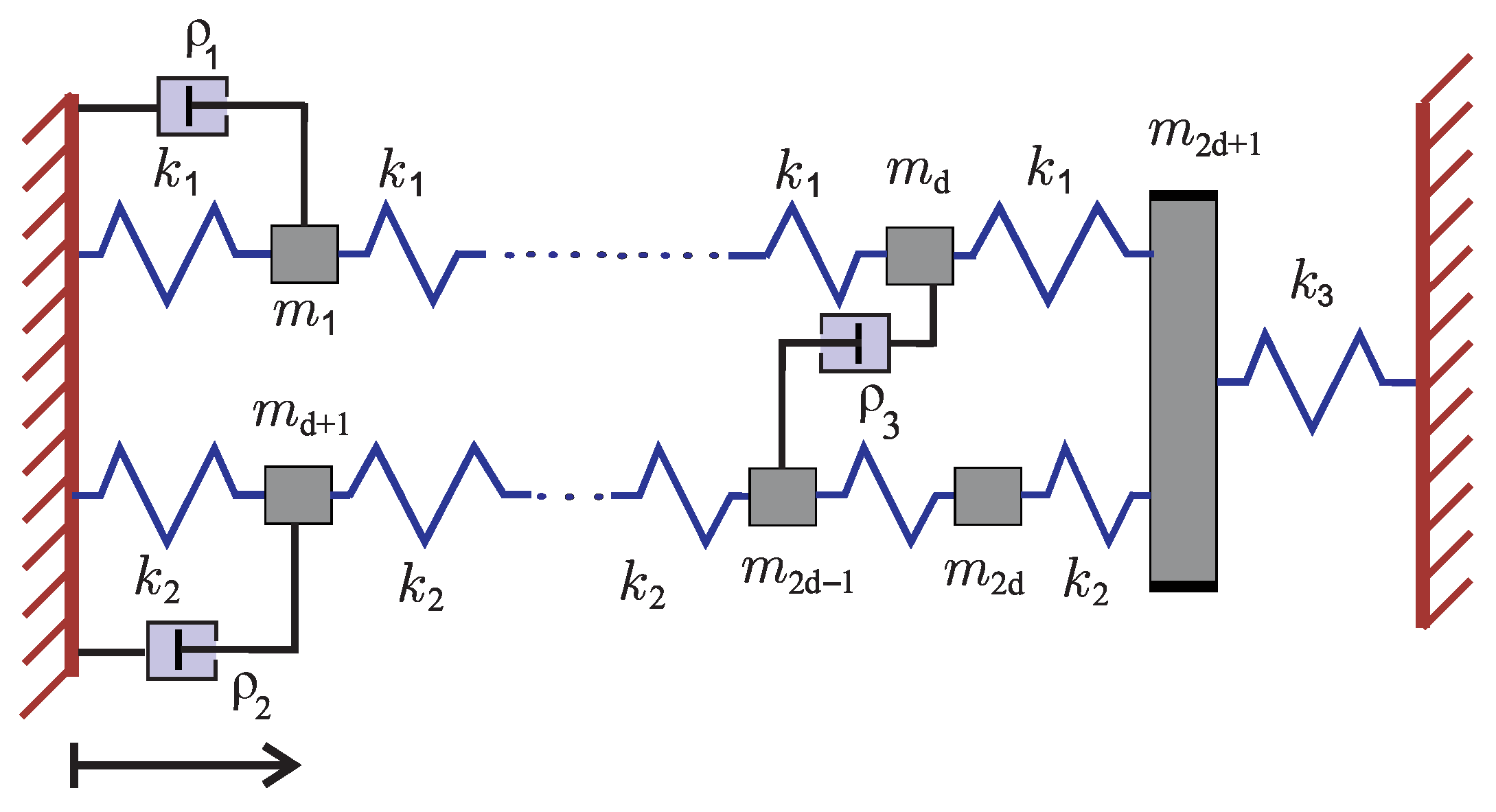
Let us describe the large example. The small example has the same structure, we just use an n-mass oscillator with a smaller number of masses. The code used to generate both examples is available in the file src/GenerateExamples.jl in the GitHub repository [42]. We consider the mechanical system shown in Figure 1. Similar examples were considered in [3,5,8,9,13,15]. In all our examples the mass oscillator contains two rows of d masses that are grounded from one side, while on the other side masses are connected to one mass which is then grounded. Therefore, we consider $2d+1$ masses and $2d+3$ springs, while the system has three dampers of different viscosities ${\rho }_1$, ${\rho }_2$ and ${\rho }_3$. However, we include several different configurations since system dimension n and parameters that determine system configuration are changed as we will describe below.

For configuration given by Figure 1, one can derive the system of differential equations that describe the behavior of displacements from equilibrium for each mass separately. In particular, for each mass one can write an equation that follows Newton’s law and describes displacement for corresponding mass. For that purpose, one should take into account that the elastic force from the neighboring springs is negatively proportional to the relative displacement and forces that arise due to the damping effects. This can be written in the matrix form using Equation (1) (see, e.g, [2]). We obtain the mass matrix

$$M=\mathrm{diag}(m_1,m_2,\dots ,m_n),$$

(45)

and the stiffness matrix

$$K=\left[\begin{array}{ccc}{K}_{11}& & -{\kappa }_1\\ & K_{22}& -{\kappa }_2\\ -{\kappa }_1^T& -{\kappa }_2^T& k_1+k_2+k_3\end{array}\right],$$

(46)

where

$$K_{ii}=k_i\left[\begin{array}{ccccc}2& -1& & & \\ -1& 2& -1& & \\ & \ddots & \ddots & \ddots & \\ & & -1& 2& -1\\ & & & -1& 2\end{array}\right],{\kappa }_i=\left[\begin{array}{c}0\\ ⋮\\ 0\\ k_i\end{array}\right],i=1,2,k_j\in \mathbb{R},j=1,2,3.$$

We consider the following configuration:

$$\begin{array}{cc}\hfill k_1& =100,k_2=150,k_3=200,\hfill \\ \hfill m_i& =2000-4i,i=1,\dots ,d/2,\hfill \\ \hfill m_i& =3i-800,i=d/2+1,\dots ,d,\hfill \\ \hfill m_i& =500+i,i=d+1,\dots ,2d,\hfill \\ \hfill m_{2d+1}& =1800\hfill \end{array}$$

for $d=800$ and $n=1601$ masses and the internal damping $D_{int}$ determined by (3) for $\alpha =0.02$. As shown in Figure 1, we consider three dampers. The first two dampers are grounded, while the third damper connects two rows of masses. This means that external damping is determined by (5) with

$$D_1=e_{i_1}{e}_{i_1}^T,D_2=e_{i_2}{e}_{i_2}^{T}and{D}_3=(e_{i_3}-e_{i_3+400}){(e_{i_3}-e_{i_3+400})}^T,$$

where $e_i$ corresponds to the i-th canonical vector.

Here, we would like to emphasize that in general one needs to determine indices $i_1$, $i_2$, $i_3$ and corresponding viscosities ${\rho }_1,{\rho }_2$ and ${\rho }_3$ such that the total average energy is minimal. As we mentioned in the introduction, here we do not consider optimization of damping positions since our main aim was to accelerate the calculation of objective function. Thus, here we fix damping positions and optimize viscosities as we state below.

In particular, here we present results for only one configuration $\left[\begin{array}{ccc}{i}_1& i_2& i_3\end{array}\right]$. We would like to damp the 27 smallest eigenfrequencies of the system, that is, the matrix G is defined by (13) with $s=27$.

In the homogeneous example $n=2001$, $M=\mathrm{diag}(m_1,m_2,\dots ,m_n)$, where the first thousand masses are $m_i=1000$, the next thousand masses are $m_i=1500$, the last mass is $m_{2001}=2000$, and

$$K=\left[\begin{array}{cccccc}200& -100& & & & \\ -100& 200& -100& & & \\ & -100& 200& & & \\ & & & \ddots & & \\ & & & & & \\ & & & & 300& -150\\ & & & & -150& 450\end{array}\right].$$

In this example we choose $s=20$ in Equation (13). The code used to generate the homogeneous example is available in the file src/GenerateExamples.jl in the GitHub repository [42].

Our problems and solutions are described in

Table 1. Description of examples. For above described examples we present: size of test problem, size of linearized problem, indices defining configuration of dampers, and resulting optimal viscosities.

Problem	Size	Linearized Size	$\left[\begin{array}{ccc}{\mathit{i}}_1& {\mathit{i}}_2& {\mathit{i}}_3\end{array}\right]$	Optimal Viscosities
Small	801	1602	$\left[\begin{array}{ccc}50& 550& 120\end{array}\right]$	$\left[\begin{array}{ccc}561.4& 651.8& 310.6\end{array}\right]$
Large	1601	3202	$\left[\begin{array}{ccc}50& 950& 220\end{array}\right]$	$\left[\begin{array}{ccc}721.1& 656.5& 415.4\end{array}\right]$
Homogeneous	2001	4002	$\left[\begin{array}{ccc}850& 1950& 20\end{array}\right]$	$\left[\begin{array}{ccc}620.0& 1047.1& 970.2\end{array}\right]$

. The timings for the standard method computed using Matlab and our new method using Julia [43] are given in

Table 2. Standard method in Matlab. For all three examples we present run times in seconds for the standard $O\left(n^3\right)$ method using Matlab with 12 cores. The individual problems are solved using the function lyap() from the SLICOT library [28], and the unconstrained optimization is performed using the function fminsearchbnd(). In the parentheses is the number of calls of the function lyap().

Problem	Lyap(SLICOT)	Optimization
Small	1.8	162 (95 calls)
Large	11.2	1050 (97 calls)
Homogeneous	22.9	2608 (109 calls)

and

Table 3. New method in Julia. For all three examples we present run times in seconds for the new $O\left(n^2\right)$ method using Julia with 12 cores. The first column displays times for eigenvalue decomposition of a CSymDPR1 matrix computed by the function Eigen() from Algorithm 2. The second column displays times for single trace computation using the function TraceX() from Algorithm 3. The third column displays times for the optimization of viscositites using the function Optimize from Algorithm 4. The optimization is performed using the function ConjugateGradient() from the Julia package Optim.jl [44]. In the parentheses is the number of calls of the function TraceX(). Our Julia programs are available on GitHub [42].

Problem	Eigen	TraceX	Optimize
Small	0.14	0.72	60 (79 calls)
Large	0.48	2.4	182 (79 calls)
Homogeneous	0.94	4.2	350 (71 calls)

, respectively. In Table 2 and Table 3, comparison is made between Matlab and Julia. Julia is known to be faster than Matlab since the functions are pre-compiled before execution. In this case we are using Matlab’s built-in function lyap(), which uses pre-compiled routines from the SLICOT library [28]. Even more, Matlab’s implementation of the SLICOT library in a multithreading environment is more than twice faster as Julia’s, so the comparison between the standard algorithm and our method is fair. To see the influence of the number of dampers, the times for single trace computation and complete optimization for 3, 4, and 5 dampers are given in

Table 4. Various number of dampers. We present timings for the large problem varying the number of dampers from three, as in Table 3, to five. The first column displays times for single trace computation using the function TraceX(). The second column displays times for the optimization of viscositites using the function Optimize(). In the parentheses is the number of calls of the function TraceX().

Number of Dampers	TraceX	Optimize
3	2.4	182 (79 calls)
4	3.25	412 (128 calls)
5	4.06	628 (154 calls)

. In

Table 5. Condition numbers, residuals and relative errors. The first column displays condition number (42) for each problem. The second column displays maximal condition number of all eigenvector matrices S and $S_1$ from (32) and (33) which appear during the entire optimization process. The third column displays maximal relative residuals of the computed solutions of the Lyapunov Equation (14) with A from (29) over the entire optimization process. The fourth column displays maximal relative errors between trace and optimal viscosities computed by our method and the standard method using Matlab’s function lyap().

Problem	$\mathit{\kappa }(\mathit{K},\mathit{M})$	$max\mathit{\kappa }\left(\mathit{S}\right)$	Residual	Relative Error
Small	$1.4\times {10}^5$	594.8	$2.6\times {10}^{-9}$	0.0008
Large	$6.3\times {10}^5$	120.2	$1.3\times {10}^{-9}$	0.0005
Homogeneous	$4.1\times {10}^5$	463.9	$1.5\times {10}^{-9}$	0.0005

, we display the norm of residuals of the computed solution X of the Lyapunov Equation (36). We also display the maximal relative errors between minimal trace and optimal viscosities computed by our method from Section 2.2 and the standard method from Section 2.1 (see also [8]), where solutions of (14) with $A\left(D_{ext}\right)$ given by (12), are computed using Matlab’s function lyap().

4. Discussion

Comparing Table 2 and Table 3, we see that the speedup of our method over the standard method grows with dimension (more precisely: 2.24, 4.03, and 4.8, computed by adjusting the number of trace computations). From Table 2 we see that the computation times for the standard method for both, individual eigenvalue computations and optimization procedure, are proportional to $O\left(n^3\right)$. Also, the computation times in Table 3 for both, individual eigenvalue decomposition from the column Eigen and trace computation from the column TraceX, are clearly proportional to $n^2$. This confirms the fact that our method is asymptotically an order of magnitude faster than the standard direct method in the typical case when the number of dampers is small.

Timings from Table 4 show that the duration of computation is indeed linearly proportional to the number of dampers, as predicted by the analysis.

The condition numbers $\kappa (K,M)$ in Table 5 govern the overall accuracy of the computation. The maximal condition numbers of all eigenvector matrices S and $S_1$ from (32) and (33) which appear during the entire optimization process are smaller than $\kappa (K,M)$, so our method does not introduce extra errors. Maximal relative residuals of the computed solutions of the Lyapunov Equation (14) with $A(D_{ext}$ from (29) over the entire optimization process, displayed in the third column of Table 5, are very small. This behavior is expected according to the analysis from Section 2.2.6. Maximal relative errors between optimal traces and optimal viscosities computed by our method and the standard method, shown in the fourth column of Table 5, are small enough, which demonstrates that our method is comparable in accuracy to the standard one.

5. Conclusions

The proposed direct algorithm, based on the fast algorithm for the solution of the eigenvalue problems for CSymDPR1 matrices and fast multiplication of Cauchy-like matrices, is simple, stable, and outperforms the standard direct counterpart, especially when the size of the problem n is large and the number of dampers k is small. It is also easy to implement in Julia’s multithreading environment.

After the initial eigenvalue decomposition of the linearized problem, our algorithm computes optimal viscosities for each choice of external dampers in $O\left(k{n}^2\right)$ operations. Hence, if the number of dampers is small, the subsequent optimization is the order of magnitude faster than in the standard approach, while maintaining accuracy.

Future work may include a more detailed analysis of the new method and development of the eigenvalue decomposition algorithm for block complex symmetric diagonal-plus-low-rank matrices, which could treat all k dampers simultaneously and, thus, be even faster.

References

- Gawronski, W.K. Advanced Structural Dynamics and Active Control of Structures; Springer: New York, NY, USA, 2004. [Google Scholar]
- Veselić, K. Damped Oscillations of Linear Systems; Springer Lecture Notes in Mathematics; Springer: Berlin, Germany, 2011. [Google Scholar]
- Veselić, K. On linear vibrational system with one dimensional damping II. Integral Equ. Oper. Theory 1990, 13, 883–897. [Google Scholar] [CrossRef]
- Cox, S.; Nakić, I.; Rittmann, A.; Veselić, K. Lyapunov optimization of a damped system. Syst. Control Lett. 2004, 53, 187–194. [Google Scholar] [CrossRef]
- Truhar, N.; Veselić, K. An efficient method for estimating the optimal dampers’ viscosity for linear vibrating systems using the Lyapunov equation. SIAM J. Matrix Anal. Appl. 2009, 31, 18–39. [Google Scholar] [CrossRef]
- Kuzmanović, I.; Tomljanović, Z.; Truhar, N. Optimization of material with modal damping. Appl. Math. Comput. 2012, 218, 7326–7338. [Google Scholar] [CrossRef]
- Müller, P.C.; Schiehlen, W.O. Linear Vibrations; Martinus Nijhoff: Dordrecht, The Netherlands, 1985. [Google Scholar]
- Benner, P.; Tomljanović, Z.; Truhar, N. Optimal damping of selected eigenfrequencies using dimension reduction. Numer. Linear Algebr. 2013, 20, 1–17. [Google Scholar] [CrossRef]
- Benner, P.; Tomljanović, Z.; Truhar, N. Dimension reduction for damping optimization in linear vibrating system. J. Appl. Math. Mech. 2011, 91, 179–191. [Google Scholar] [CrossRef]
- Freitas, P.; Lancaster, P. On the optimal value of the spectral abscissa for a system of linear oscillators. SIAM J. Matrix Anal. Appl. 1999, 21, 195–208. [Google Scholar] [CrossRef]
- Nakić, I.; Tomljanović, Z.; Truhar, N. Optimal Direct Velocity Feedback. Appl. Math. Comput. 2013, 225, 590–600. [Google Scholar] [CrossRef]
- Nakić, I. Optimal Damping of Vibrational Systems. Ph.D. Thesis, Fernuniversität, Hagen, Germany, 2002. [Google Scholar]
- Truhar, N.; Tomljanović, Z.; Puvača, M. An Efficient Approximation For Optimal Damping In Mechanical Systems. Int. J. Numer. Anal. Model. 2017, 14, 201–217. [Google Scholar]
- Benner, P.; Denißen, J. Numerical solution to low rank perturbed Lyapunov equations by the sign function method. Proc. Appl. Math. Mech. 2016, 16, 723–724. [Google Scholar] [CrossRef] [Green Version]
- Kanno, Y.; Puvača, M.; Tomljanović, Z.; Truhar, N. Optimization of Damping Positions in a Mechanical System. Rad HAZU 2019, 23, 141–157. [Google Scholar]
- Nakić, I.; Tomljanović, Z.; Truhar, N. Mixed control of vibrational systems. J. Appl. Math. Mech. 2019, 99, 1–15. [Google Scholar] [CrossRef] [Green Version]
- Xu, B.; Wu, Z.; Chen, G.; Yokoyama, K. Direct identification of structural parameters from dynamic responses with neural networks. Eng. Appl. Artif. Intell. 2004, 17, 931–943. [Google Scholar] [CrossRef]
- Bai, Z.; Su, Y. SOAR: A second-order Arnoldi method for the solution of the quadratic eigenvalue problem. SIAM J. Matrix Anal. Appl. 2005, 26, 640–659. [Google Scholar] [CrossRef] [Green Version]
- Guo, C.H. Numerical solution of a quadratic eigenvalue problem. Linear Algebra Appl. 2004, 385, 391–406. [Google Scholar] [CrossRef]
- Tisseur, F.; Meerbergen, K. Quadratic eigenvalue problem. SIAM Rev. 2001, 43, 235–286. [Google Scholar] [CrossRef] [Green Version]
- Li, J.R.; White, J. Low rank solution of Lyapunov equations. SIAM J. Matrix Anal. Appl. 2002, 24, 260–280. [Google Scholar] [CrossRef]
- Penzl, T. LYAPACK. Available online: http://www.tu-chemnitz.de/sfb393/lyapack (accessed on 20 May 2021).
- Benner, P.; Quintana-Ortí, E.S. Solving Stable Generalized Lyapunov Equations with the Matrix Sign Function. Numer. Algorithms 1999, 20, 75–100. [Google Scholar] [CrossRef]
- Kenney, C.; Laub, A.J. The Matrix Sign Function. IEEE Trans. Automat. 1995, 40, 1330–1348. [Google Scholar] [CrossRef]
- Hammarling, S.J. Numerical solution of the stable, nonnegative definite Lyapunov equation. IMA J. Numer. Anal. 1982, 2, 303–323. [Google Scholar] [CrossRef] [Green Version]
- Kressner, D. Block variants of Hammarling’s method for solving Lyapunov equations. ACM Trans. Math. Softw. 2008, 34, 1–15. [Google Scholar] [CrossRef]
- Bartels, R.H.; Stewart, G.W. A solution of the matrix equation AX + XB = C. Comm. ACM 1972, 15, 820–826. [Google Scholar] [CrossRef]
- SLICOT, Subroutine Library in Systems and Control Theory. Available online: http://slicot.org/ (accessed on 12 June 2021).
- Pan, V.Y.; Zheng, A. Superfast algorithms for Cauchy-like matrix computations and extensions. Linear Alg. Appl. 2000, 310, 83–108. [Google Scholar] [CrossRef] [Green Version]
- Watkins, D.S. Unsymmetric Matrix Eigenvalue Techniques. In Handbook of Linear Algebra; Hogben, L., Ed.; CRC Press: Boca Raton, FL, USA, 2014; Volume 56, pp. 1–12. [Google Scholar]
- Cuppen, J.J.M. A divide and conquer method for the symmetric tridiagonal eigenproblem. Numer. Math. 1981, 36, 177–195. [Google Scholar] [CrossRef]
- Golub, G.H.; Van Loan, C.F. Matrix Computations, 4th ed.; The John Hopkins University Press: Baltimore, MD, USA, 2013. [Google Scholar]
- Bini, D.A.; Fiorentino, G. Design, analysis, and implementation of a multiprecision polynomial rootfinder. Numer. Algorithms 2000, 23, 127–173. [Google Scholar] [CrossRef]
- Multiprecision Polynomial SOLVEr (MPSolve). Available online: https://numpi.dm.unipi.it/software/mpsolve (accessed on 14 May 2021).
- Jakovčević Stor, N.; Slapničar, I.; Barlow, J.L. Forward stable eigenvalue decomposition of rank-one modifications of diagonal matrices. Linear Algebra Appl. 2015, 487, 301–315. [Google Scholar] [CrossRef]
- Parlett, B.N. The Rayleigh quotient iteration and some generalization for nonnormal matrices. Math. Comput. 1974, 28, 679–693. [Google Scholar] [CrossRef]
- Arbenz, P.; Hochstenbach, M.E. A Jacobi–Davidson method for solving complex symmetric eigenvalue problems. SIAM J. Sci. Comp. 2004, 25, 1655–1673. [Google Scholar] [CrossRef] [Green Version]
- Pan, V.Y.; Zheng, A. New progress in real and complex polynomial root finding. Comput. Math. Appl. 2011, 61, 1305–1334. [Google Scholar] [CrossRef] [Green Version]
- Higham, N.J. Accuracy and Stability of Numerical Algorithms, 2nd ed.; SIAM: Philadelphia, PA, USA, 2002. [Google Scholar]
- Slapničar, I. Symmetric Matrix Eigenvalue Techniques. In Handbook of Linear Algebra; Hogben, L., Ed.; CRC Press: Boca Raton, FL, USA, 2014; Volume 55, pp. 1–26. [Google Scholar]
- Drmač, Z. Computing Eigenvalues and Singular Values to High Relative Accuracy. In Handbook of Linear Algebra; Hogben, L., Ed.; CRC Press: Boca Raton, FL, USA, 2014; Volume 59, pp. 1–20. [Google Scholar]
- FastOptimalDamping.jl. Available online: https://github.com/ivanslapnicar/FastOptimalDamping.jl (accessed on 10 February 2022).
- The Julia Language. Available online: http://julialang.org/ (accessed on 10 February 2022).
- Julia Package Listing. Available online: http://pkg.julialang.org/ (accessed on 10 February 2022).
Figure 1.
mass oscillator.