
Hierarchical Reinforcement Learning: A Survey and Open Research Challenges


Department of Computer Science, University of Antwerp—imec, Sint-Pietersvliet 7, 2000 Antwerp, Belgium
*
Author to whom correspondence should be addressed.
Mach. Learn. Knowl. Extr. 2022, 4(1), 172-221; https://doi.org/10.3390/make4010009
Submission received: 10 December 2021
/
Revised: 21 January 2022
/
Accepted: 8 February 2022
/
Published: 17 February 2022
(This article belongs to the Special Issue Advances in Reinforcement Learning)
Abstract
:Reinforcement learning (RL) allows an agent to solve sequential decision-making problems by interacting with an environment in a trial-and-error fashion. When these environments are very complex, pure random exploration of possible solutions often fails, or is very sample inefficient, requiring an unreasonable amount of interaction with the environment. Hierarchical reinforcement learning (HRL) utilizes forms of temporal- and state-abstractions in order to tackle these challenges, while simultaneously paving the road for behavior reuse and increased interpretability of RL systems. In this survey paper we first introduce a selection of problem-specific approaches, which provided insight in how to utilize often handcrafted abstractions in specific task settings. We then introduce the Options framework, which provides a more generic approach, allowing abstractions to be discovered and learned semi-automatically. Afterwards we introduce the goal-conditional approach, which allows sub-behaviors to be embedded in a continuous space. In order to further advance the development of HRL agents, capable of simultaneously learning abstractions and how to use them, solely from interaction with complex high dimensional environments, we also identify a set of promising research directions.
1. Introduction
Reinforcement learning (RL) [1,2] is a powerful method for solving sequential decision-making problems. RL agents are capable of learning how to solve a problem from interactions with its environment. In order to solve the problem, the agent does not need to know the dynamics of the environment in advance. A successful RL system will efficiently utilize experience gathered during trial-and-error learning, in order to maximize an external training-signal, called the reward-signal.
Combining RL with recent advancements in the area of deep learning [3,4] has had a big impact on RL, giving birth to a new subfield called deep reinforcement learning [5,6,7,8]. Deep RL applies RL techniques, using high-dimensional state-spaces, such as images [9] and natural language [10]. This has been made possible because of the capability of deep learning algorithms to introduce different learnable layers of abstractions on the raw input data. For example, the DQN algorithm [8], and more recently PPO [11] Rainbow [12], and Atari57 [13] are RL algorithms that are capable of achieving above human-level performance on a set of classic Atari 2600 video games. These approaches are able to distill a highly performing behavior by directly using the screen pixels. Other recent successes of deep RL include beating top professional human players in the complex board game of Go [14], and achieving human level performance in cooperative 3D multiplayer video games such as DOTA 2 [15,16], StarCraft II [17] and a modified version of Quake III Arena [18].
There has also been significant progress towards applying deep RL in real-world applications such as robotics [19,20,21,22,23,24], dialog management systems [25], education [26], autonomous vehicles [27,28] smart grids [29], fleet management [30], resource management [31,32] and recommender systems [33]. However, building real-world RL applications still remains challenging [34], because RL algorithms struggle with being sample efficient [35,36,37,38], that is, being able to learn a satisfying behavior, from a limited amount of interaction with the environment. Furthermore, real-world RL systems require hard constraints in order to not damage equipment and allow safe exploration [39,40]. Real-world RL systems will also need to be capable of handling real-time systems, allowing states and actions to evolve simultaneously [41,42,43], which is different from the commonly used turn-by-turn environment interactions.
Hierarchical reinforcement learning (HRL) extends the capabilities of RL, by proposing a divide-and-conquer approach. In this approach, the complex, difficult to solve problem, is abstracted into multiple smaller problems. These abstracted problems are generally easier to solve and their solutions can be reused to solve different problems. This approach has previously been successfully utilized [44,45,46] to speed up many offline planning algorithms where the dynamics of the environment are known in advance.
This compositionality has been identified [1,47] as one of the key building blocks of artificial intelligence. Humans intuitively harness compositionality in order to tackle complex problems. For example, planning a vacation can be a complex endeavour if considered as a whole. However, when decomposed into multiple smaller tasks (e.g., selecting a hotel, booking a flight, arranging transportation to the airport) the task becomes more manageable. Efficiently using such abstractions has proven to make significant contributions towards solving various important open RL problems such as reward-function specification, exploration, sample efficiency, transfer learning, lifelong learning and interpretability.
An essential part of RL algorithms is that they use feedback in order to learn what is good and bad behavior. When feedback in the form of a reward signal is abundantly available, an agent can learn quickly. Unfortunately, specifying such dense reward signals is a complex challenge [48], and often results in unwanted side effects. Moreover, most control problems naturally come with a sparse reward signal (e.g., object grasped, destination reached). A sparse reward formulation makes learning extremely challenging as there is mostly only information on what does not work. Hierarchical reinforcement learning (HRL) often utilizes various forms of intrinsic motivation [49] in order to provide additional denser reward signals for individual abstractions.
A second open challenge in RL has been how to explore the environment efficiently [50,51,52,53]. Recent empirical research [54] demonstrated that even simple forms of temporally correlating actions, improves exploration efficiency. In this research, temporally extended exploration is seen as one of the most important contributions of HRL.
Reinforcement learning (RL) systems are also notoriously known for their sample inefficiency. While efficient use of abstractions seems a promising solution to this long-standing challenge, increased sample efficiency through HRL is most commonly only realized when amortizing computation over multiple iterations of very similar problems. Off-policy learning [37,55,56] is a popular approach towards making RL more sample efficient. HRL algorithms unfortunately typically still require a more stable on-policy approach.
Current RL algorithms focus mostly on solving only a single problem. However, abstractions that can be re-used when solving different tasks, pose a possible answer to the question of transfer learning in RL [57]. Drawing inspiration from research done in deep learning on how to transfer visual representations from one task to another [58,59], HRL methods have shown to be capable of learning transferable abstractions within the same problem setting [60]. However, how to transfer abstractions between very different problems remains an open problem.
Hierarchical reinforcement learning (HRL) algorithms are also considered an important step for building lifelong-learning agents [47,61,62]. These agents are capable of extending and managing their knowledge, in order to become more efficient in solving ever more complex problems.
Generally, RL systems suffer from being opaque to humans [63,64,65]. Various forms of abstractions used in HRL could allow an increased interpretability.
While the potential of HRL is vast, automatically discovering abstractions is non-trivial and remains an open research question. A lot of progress has been made recently, utilizing various forms of temporal and state abstractions. However, solutions currently either heavily depend on expert knowledge, do not scale well, or are sample inefficient.
The goal of this paper is to provide RL researchers a comprehensive understanding of how various HRL algorithms contribute towards solving the above described open challenges in RL. While initial steps in HRL have been previously surveyed [66], the capability of deep learning to work with high dimensional data has inspired a whole new set of directions and possibilities in HRL. For example, the challenge of end-to-end discovering, and sequencing temporally extended actions, directly from high dimensional inputs, is a novel direction which has become possible because of recent breakthroughs in deep learning. While also briefly covering early research, the focus of this survey is on these new directions inspired by deep learning.
This paper first introduces the typically utilized formalism in Section 2. Afterwards in Section 3 the core challenges of HRL are discussed. The largest part of this paper consists of a survey of three frameworks and their most common implementations (problem-specific models in Section 4, options in Section 5, and the goal-conditional framework in Section 6). An overview of benchmark environments and tasks used in HRL is provided in Section 7. We provide an evaluation of the discussed frameworks and algorithms in Section 8. In order to spark future research, we also provide a list of future research directions in Section 9.
2. Background
In this section we briefly present the formal framework which is typically used to describe RL problems and HRL agents.
2.1. Markov Decision Processes
A Markov Decision Process (MDP) [67] is a formal model, used to describe discrete-time stochastic control processes. The MDP model is useful for representing decision-making problems in which an agent can influence the process by executing actions.
A MDP is defined by a tuple , in this tuple:
- defines the set of possible states the agent can be in, also called the state-space,
- contains the set of actions the agent can execute, also called the action-space,
- is the transition function. This function determines what the outcome-state of an action in a state will be. This function is also often called the environment-model.
- is the reward-function, an agent can receive reward when visiting certain states.
The agent exercises control over the MDP by executing actions. A solution to an MDP can be expressed with a policy . This policy models which action the agent takes, given a state: . The objective in an optimal control problem is to find an optimal policy that maximizes the return, which is defined as the expected accumulated reward along a trajectory.
Typically, the state of the MDP is reset after a finite number of T-steps. This is called an episodic MDP. In a non-episodic MDP . The sequence of states, actions and rewards collected during a single instance of an episode is considered a trajectory .
In a MDP, the probability of future state transitions only depends on the current state. This assumption is called the Markov-property. In practice this entails that the current state should contain all the information an agent needs to make optimal action decisions. And thus the agent does not require the usage of a memory of past states.
The received reward is often discounted using a discount factor . Reward received in the future is often less valuable to the agent than reward we can receive immediately. If this also entails that cumulative rewards of trajectories are finite. This is especially important when the MDP is non-episodic, and can go on forever.
Semi-Markov Decision Processes
In the MDP framework an action is taken on each discrete time step. This means that each action exactly takes the same amount of timesteps to execute. However, when working in a continuous time space, or when dealing with temporally extended sequences of actions, which is often the case in HRL, different actions might have different execution lengths, as demonstrated in Figure 1.
In order to support variable duration of a single action, the MDP framework has been extended to the Semi-Markov Decision Process (SMDP) framework [68,69,70]. This was done by adding an additional random variable T to the transition-function . This random variable denotes the time between actions. In the case of a SMDP the reward-function denotes the cumulative reward collected during T steps after executing in .
2.2. Reinforcement Learning
Assuming full knowledge of the MDP, techniques such as dynamic programming [71] can be utilized to derive an optimal policy . However, full knowledge of the underlying MDP is often an unrealistic assumption. In most sequential control processes, the transition-function of the MDP is unknown.
Reinforcement learning (RL) [1] is the problem set, concerned with handling unknown factors in the MDP, by utilizing a trial-and-error approach. A RL agent starts in an initial state . At each time step t the agent interacts with the environment by taking an action . The agent can either act greedy, and exploit what it already has learned by following its current policy . Alternatively, the agent can also choose to explore the outcome of a different random action in order to possibly learn a better policy. This distinctive interaction between agent and environment is pictured in Figure 2.
Balancing this explore/exploit trade off is one of the characteristic problems of RL. Different exploration schemes exist. For example, by adding noise to the action-space, -greedy takes random actions of the time. The parameter is often decayed over a number of steps. Other exploration schemes add noise directly to the policy parameters [72,73], add an intrinsic curiosity bonus to the reward signal [50,51,53,74], or use a distributional perspective [75,76].
After taking action , the agent gets feedback in the form of a reward-signal , and a new state . The credit assignment problem [77] is concerned with figuring out which of the previously taken action (or set of actions) leads to a reward-signal.
The reward an agent receives directly from the environment is called the extrinsic reward. Extrinsic, because it is external to our agent. These reward signals can be dense or sparse. An open field in which the agent gets the distance to the goal-state after each action is an example of an environment with a dense reward-signal. Alternatively, if the agent only receives feedback upon reaching the goal-state, the reward is sparsely observed. An environment with a dense reward-structure makes the credit assignment problem more tractable. However, in most realistic environments, non-zero rewards are often only sparsely observed.
Most RL agents learn a policy either indirectly by learning a value function first (Section 2.2.1), or directly by searching the policy space (Section 2.2.2).
2.2.1. Value-Based Methods
The indirect RL approach uses a value function . This function is capable of estimating the cumulative discounted future reward (the value) starting from state s and following policy :
If the agent has access to the dynamics of the environment , and the state-space is small and discrete, the agent can maximize its expected cumulative future reward by navigating to the state that is within the agent’s reach and has the highest expected value.
However, most of the time, the environment dynamics are unknown, and an agent cannot reliably know what the result state will be after taking action . This is especially the case when the environment is stochastic in nature. In order to decide what action to take given the current state , a state-action-value function (or Q-function) is often used. This Q-function represents the estimated cumulative future discounted reward of taking an action a in state s while following policy :
The goal of the agent is to come as close as possible to the optimal Q-function. The optimal Q-function (), is capable of outputting the maximum achievable cumulative reward, starting in state s, and taking action a.
This Q-function can be learned, using algorithms such as the off-policy Q-Learning [78] algorithm or the on-policy SARSA algorithm [79]. An on-policy algorithm updates a policy only with samples gathered by utilizing this policy. Off-policy learning is typically more sample-efficient, as it also is capable of utilizing experiences gathered when following a different policy (for example a policy which explores more) and re-using past experiences gathered by utilizing previous versions of the policy.
Q-learning is considered off-policy, because it does not use the current policy to estimate the total value of the next state , but instead uses the highest expected value.
While SARSA is considered on-policy because it uses the current policy to sample the next action :
In order to actually learn the Q-function from interaction with the environment, both Q-learning and SARSA use a Bellman equation [71], which recursively allows updating Q-values:
Once the agent has iteratively learned a good estimate of from interaction with the environment (value iteration), a greedy policy can be derived:
2.2.2. Policy Gradient Methods
An alternative family of policy gradient methods directly search for an optimal policy in the policy space, by using gradient descent on the total expected future value objective function .
This family of algorithms typically utilizes policy iteration. In policy iteration, the agent alternates between an evaluation phase, and a phase in which the policy is updated according to the received feedback.
For example, the REINFORCE family of algorithms [80] searches for the parameters of by using the gradient:
In practice, these types of algorithms try out different actions, and increase the likelihood that the policy will sample successful actions again, when in similar states.
Unfortunately calculating is non-trivial because the dynamics of the environment are generally unknown. The policy gradient theorem [81] allows the policy gradient to be represented as an expectation.
This allows the gradient to be calculated from environment interactions:
In order to perform this policy improvement step, the agent needs an estimate of the total future value of an action in a state . In order to obtain such value-estimation, Monte Carlo simulation can be utilized to estimate total future value from entire trajectories. Because gradients obtained by sampling trajectories are often subject to high variance, it is also common to instead of estimating the value function, to use a baseline, in order to obtain a function with a lower estimation variance.
A simple baseline would be to subtract an average reward, obtained over a number of episodes. An advantage function is also often used, using the total future value of the state as the baseline:
In order to facilitate exploration an entropy regularizer is often used, facilitating stochastic behavior of the policy.
Policy gradient methods have also been combined with value function estimation methods. This approach is called Actor-Critic [82]. This family of methods uses policy gradients to optimize a parameterized policy (the actor), while simultaneously deriving a value function (the critic), in order to reduce the variance of policy gradient methods.
2.3. Deep Reinforcement Learning
When the state and action-space are limited and discrete, elements of a RL architecture (such as the policy, and/or value estimations), can be represented using a low-dimensional matrix. However, this method quickly becomes intractable for more complex problems, utilizing high-dimensional input data such as images or audio. Various function approximation methods have been used in the past in order to represent different components of a RL agent. Example function approximation techniques include: linear models that learn individual expert-provided features of the state-space [83], and tree-based algorithms [84].
Recently deep neural networks have demonstrated to be capable of learning useful hierarchies of task-specific representations from raw high-dimensional input signals [3,4]. These representations can be used to perform complex machine learning tasks end-to-end such as image classification [85,86,87,88], image captioning [89], visual question answering [90], image generation [91,92,93], sound generation [94], object detection [95,96], speech recognition [97,98,99,100], natural language translation [94,101], and natural language understanding [102,103]. These techniques are also starting to be utilized by industries such as agriculture [104] and medicine [105].
The progress made in the area of deep learning has been made possible by a few building blocks. For example, in computer vision applications, convolutional neural networks [106] have been demonstrated to be capable of capturing task-specific spatial and temporal dependencies. In such a network each layer uses filters in order to extract learned high-level features from the input in order to provide a lower dimensional representation as the original input to the downstream task (e.g., image classification or MDP value estimation).
Building blocks such as Long Short-Term Memory (LSTM) [107] recurrent networks and Gated Recurrent Units (GRU ([108] allow deep learning to work with data which is sequential in nature. To accomplish this, they use gates which are capable of learning which parts of the sequential input data, summarized in a hidden state, should be passed on, and what to forget. These techniques are especially interesting when working with natural language, as the meaning of a word in a sentence is often dependent on other neighboring words. However, in RL too, memory can be useful, or even required, when the current non-Markovian state does not contain all information required to make an optimal action decision.
However, when sequences become longer, LSTM and GRU based approaches struggle due to their reliance on a single fixed-length vector to represent a long sequence of previous inputs. Attention [109] is a mechanism introduced to solve this problem. When using Attention, instead of relying on a single hidden state, representing past members of a sequence, attention mechanisms learn how to weigh different hidden states associated with different past sequence members. More recently transformer architectures [110] solely rely on this attention mechanism and eliminate the usage of recurrent networks. This also allows for faster inference, as inputs can now be processed in parallel.
Also, unsupervised deep learning approaches, capable of generating new previously unseen data instances have recently achieved tremendous successes, and have been added to the standard set of deep learning building blocks. These techniques include Variational Autoencoders (VAE) [111], which utilize a regularized bottleneck autoencoder approach. A regular autoencoder [112] encodes a high-dimensional input in a lower dimensional latent space. The VAE regularization tries to make sure that points close in the latent space are also similar once decoded back into their high-dimensional form. This regularization allows the generation of new data instances by generating points in the latent space.
Generative Adversarial Networks (GAN) [113] generate new data using a generator network, which receives feedback whether the generated instances look realistic by a second discriminator network. This approach has been demonstrated to be capable of generating out-of-sample high dimensional images [91] indistinguishable from real photographs.
While research in deep learning has focussed on processing high dimensional inputs such as image data and natural language, alternative forms of data have been studied. For example, Graph Neural Networks (GNN) [114,115] are capable of directly working with data structured as a graph.
One of the key challenges in RL is to be able to generalize feedback received from the environment to unvisited states, and untested actions. Using deep neural networks we can learn representations from raw high-dimensional input-spaces, which in turn can be used to approximate value functions, or directly express a policy. Unfortunately, combining non-linear function approximation, and iterative value function bootstrapping is prone to unstable learning [116,117], especially in an off-policy setting. This problem has been identified as the deadly triad of RL [1].
The seminal work of Mnih et al. [8] demonstrated above human-level performance on a set of classic Atari 2600 video-games [118]. The introduced off-policy Deep Q-Network (DQN) architecture was able to learn different policies for a range of different video games, using only pixels as input data. In order to generalize collected experience to unseen states, and untested actions, the function is represented using a deep neural network. The issue of instability caused by function approximation in RL [119] was tackled by the usage of a separate target network, used to predict next-state future values. This target network is only periodically updated. Additionally, an experience replay buffer [120,121] was used, in order to reduce temporal correlation in the observed state-reward sequences.
The DQN algorithm has been heavily studied, and various improvements have been proposed such as Double Q-Learning (DDQN) [122], prioritized replay [123], dueling networks [124], multi-step learning [125] and distributional RL [75,76,126]. The Rainbow framework [12] combines these improvements. While the original DQN-architecture could not achieve above-human performance on all tested games, the Agent57 approach [13], outperforms humans in all proposed test games, by automatically parameterizing a family of policies.
Various algorithms that directly optimize a parameterized policy such as Deep Deterministic Policy Gradient (DDPG) [127], Trust Region Policy Optimization (TRPO) [128] and Proximal Policy Optimization (PPO) [11] have also been able to work directly on high-dimensional input spaces using deep neural networks. In order to stabilize learning, policy improvements are often restricted in order to avoid making too big updates, which could collapse performance.
3. Hierarchical Reinforcement Learning
State-of-the-art deep RL algorithms require enormous amounts of interaction with the environment, before learning a satisfying control policy. Human intelligence in contrast, typically only requires a fraction of the required training experience, in order to solve the same tasks.
Lake et al. [47] identified compositionality, the idea that new representations can be constructed through the combination of primitives, as one of the core building blocks of human intelligence, and suggested that it will also be of quintessential importance in order to advance artificial learning systems. Compositionality can be seen as a way to facilitate lifelong learning [62], learning new concepts, by combining previously learned primitives [129]. In addition, the power of compositionality to come up with, seemingly unlimited new concepts, based on meaningful primitives cannot be underestimated.
HRL aims to achieve compositionality, by learning reusable sub-behaviors together with a composition strategy. While compositionality in HRL can be achieved in low-dimensional state-spaces, deep neural networks have been demonstrated to be capable of automatically discovering composable representations, which offer significant opportunities for HRL, to facilitate compositionality directly using high-dimensional inputs.
In this section, we first describe the various mechanisms that HRL utilizes in order to achieve this (Section 3.1), how this benefits RL (Section 3.2) and which challenges a modular RL approach entails (Section 3.3).
3.1. Mechanisms
3.1.1. Temporal Abstractions
One of the core mechanisms of HRL are temporal abstractions. Solving complex problems often involves reasoning on multiple time scales. For example, when driving to work you typically do not start planning about whether you should steer left or right. You start on a much higher level, by planning for example about what roads to take, and whether you should stop to refuel.
A temporally extended action (sub-behavior), consists of a sequence of primitive actions and possibly other temporally extended actions. These temporal abstractions can be utilized by a learning agent in order to make decisions on a higher level of abstraction. The sequence of actions that make up a temporally extended action can be fixed, or governed by a policy.
3.1.2. State Abstractions
A second form of abstraction that is common in HRL, are abstractions imposed on the state-space [130]. It is not feasible to learn the best action in every possible state in a high-dimensional input space. Instead, we use state abstractions (e.g., enemy visible on screen?), to reason about what action to take. Appropriate state abstractions have been demonstrated to significantly increase learning performance in RL problems [83,131].
For example, similar states in terms of transition dynamics and reward function, measured using the notion of bisimulation [132] for MDPs, can be grouped to build state abstractions [133]. These can be used to transfer an optimal policy from one MDP to a larger one [134] and to discover temporal abstractions [135].
Current deep RL algorithms are capable of learning their own state abstractions from raw high dimensional state-spaces. These algorithms are for example capable of detecting doors, and learn that it is beneficial to walk through these doors. Unfortunately, these learned state representations are often not sufficiently expressive to reason about complex environments, and develop long-horizon plans. Such a plan might for example be to search for a key, and return to the current location when confronted with a locked door.
Given abstractions over the state-space, and linked temporally extended actions, the agent can reason on a higher-level about the decisions it can make. Instead of learning a behavior for controlling the entire raw state-space, a hierarchy of different systems is able to control various abstracted parts of the state-space through temporally extended actions. An example of such a hierarchy is presented in Figure 3.
Anders and Andrew [136] identified the benefit of utilizing different state abstractions for different sub-behaviors. The intuition behind this idea is that when performing different sub-behaviors, other aspects of the state-space become relevant. Ignoring irrelevant features to the sub-behavior, allows for more efficient exploration, and learning of the different temporal abstractions.
3.2. HRL Advantages
Using both temporally extended actions and state abstractions, HRL is capable of providing significant improvements in various open RL challenges, such as credit assignment, exploration and continual learning.
3.2.1. Credit Assignment
The issue of credit assignment is a long-standing challenge in RL. Credit assignment is tasked with figuring out which action had which impact on the overall perceived reward.
Temporal and state abstractions can greatly increase the sample efficiency of RL by making credit assignment less challenging. Given a set of temporal abstractions, the agent is freed from the complexity of having to reason about which action to take on every individual step. The agent instead activates temporal abstractions which can run for multiple steps. When performing credit assignment by learning a value function, this has a profound effect on the efficiency of the value-backups [137,138]. While utilizing primitive actions only, a value backup only goes back one step, thus when reaching a goal-state, only the expected future value of the previously visited state gets updated. Using temporal abstractions, this reward gets propagated further back, allowing faster learning of a value function. This idea is demonstrated in Figure 4.
3.2.2. Exploration
While improved sample efficiency through more structured credit assignment is capable of solving RL problems which previous flat RL algorithms could not solve. A recent ablation study [54], empirically demonstrated that the most significant contribution of current HRL architectures, lies in its capability to explore in a semantically meaningful and temporally extended fashion (Figure 5). Exploration, using only primitive actions often results in over-exploration of states near the starting state of the agent. Using temporal abstractions for exploration allows the agent to explore the environment in a more structural way, which allows the agent to also explore more difficult to reach states.
However, the opposite has also been observed. Given a suboptimal set of sub-behaviors, pathological exploration can easily worsen learning performance [139].
3.2.3. Continual Learning
Problems in RL are most of the time solved from scratch, starting without any prior information. While finding a learning algorithm, capable of solving problems requiring long-term planning, without any priors, is certainly an interesting research direction. In the short-term the sample efficiency of RL can greatly be improved by building upon previously learned knowledge [47].
A policy learned without any abstractions is very difficult to transfer to a new problem (e.g., use a set of steering directions to navigate to a different location). In contrast, once learned, sub-behaviors can be transferred to solve different problems in similar environments [61,140,141,142]. Thus, the cost associated with learning sub-behaviors should not only be weighted on a single task, but should possibly be considered over multiple tasks.
3.3. HRL Challenges
Learning algorithms that utilize hierarchical compositions of temporally extended actions will have to define how these sub-behaviors should be discovered, how they can be developed, how efficient state-abstractions can be learned and how they can be composed. In this section, we briefly describe these challenges.
3.3.1. Automatic Discovery of Abstractions
Early HRL approaches [145,146,147] utilized manually defined sub-behaviors. While they demonstrated performance increases by using sub-behaviors, the requirement of manually defining sub-behaviors heavily limited their scalability.
One of the most important questions of HRL consists of: how can we automatically discover meaningful sub-behaviors? A lot of empirical research (e.g., [140,148,149,150]) has been conducted on algorithms that are capable of automatically learning meaningful sub-behaviors, from interaction with the environment, without any knowledge provided by an external expert, in a sample efficient way. Theoretically, it has been proven [151], that finding a small set of sub-behaviors in a limited number of steps is an NP-hard problem. Abel et al. [152] studied which sets of state abstractions and temporal abstractions are capable of preserving representation of near-optimal policies. However, this method requires access to the underlying MDP.
In low-dimensional environments, a small discrete set of sub-behaviors can greatly improve the sample efficiency of the learning algorithm. However, in truly complex environments, a large continuous range of sub-behaviors will be required.
3.3.2. Development of Abstractions
In order to use temporally extended actions, they need to receive enough suitable samples from the environment in order to become sufficiently developed.
In the most promising HRL approaches, sub-behaviors are developed end-to-end, while they are also being discovered [140,149,150]. This however does not need to be the case. Sub-behaviors can also be discovered and trained using a staged approach [61,154,156]. For example: the state-space could be split in a few equal parts, with a sub-behavior assigned to each part. In a second phase, the sub-behaviors can be developed by for example randomly activating them. However, as the number of sub-behaviors increases, more efficient development strategies will be required to make sure that all sub-behaviors are sufficiently trained. If multiple sub-behaviors are generalized by a single parameterized function, samples can be used to train multiple sub-behaviors at the same time. Similarly, off-policy methods can be used to simultaneously develop multiple abstractions [137].
3.3.3. Decomposing Example Trajectories
Often, it is possible to obtain human demonstrations for different control tasks. HRL can maximize the utility of such demonstrations by decomposing them into sub-behaviors. Instead of learning a single task from demonstrations, the discovered sub-behaviors can be used as building blocks to solve a range of related tasks, potentially without the need of additional demonstrations.
In imitation learning [157,158,159,160], the exploration problem of RL is made somewhat less complex, because the agent is equipped with a set of demonstration trajectories, which originate from a better than random agent (e.g., a human domain expert). While imitation learning typically is used to solve a single problem, if imitation learning is used to discover temporal abstractions, these abstractions might be re-used to solve multiple similar problems [161,162,163].
Providing a reward-function for a control problem is often a complex issue in itself [48]. The idea of Inverse Reinforcement Learning (IRL) [164,165] is that instead of manually specifying a reward-function an agent should instead learn this reward-function by observing demonstrations from an extrinsic agent. However, learning a single reward-function for the entire problem is often too coarsely defined, or demonstrations might originate from a set of different reward-functions, instead of one (e.g., when purely exploring multiple sub-behaviors). A single reward-function might also be task- or environment-specific, and not allow generalization over multiple problems. Hierarchical IRL aims to learn a composition of multiple smaller reward-functions, which can in turn be used to train sub-behaviors using trial-and-error learning techniques [166,167].
3.3.4. Composition
Sub-behaviors alone are not enough to solve HRL problems. They need to be composed in order to form complex plans. A capable HRL algorithm will need to be able to select a favorable sub-behavior to use given a state.
There are two major approaches which are commonly used to learn compositions:
- Bottom-up training: the sub-behaviors are discovered and developed first. Once they have been sufficiently developed, they are frozen, and a composition-policy is learned by sampling different sub-behaviors. This is the most straightforward way, as the higher level does not need to take into account that the outcome of the selected temporal extended actions might have changed. Sub-behaviors learned using a bottom-up approach, can often also be transferred to solve similar problems. However, in the first phase, time might be spent learning sub-behaviors which the higher-level actually does not need.
- Top-down training: the higher-level first selects a subgoal it deems interesting in order to reach the overall goal. Once selected, the lower-level is trained to reach the proposed subgoal. This approach is often more efficient, compared to training bottom-up in solving a single control problem. However, it needs to take non-stationary sub-behaviors into account. It is also often not straight-forward to transfer sub-behaviors to different problems.
4. Problem-Specific Models
Initial research on HRL agents was focused on proving the benefits of using temporal abstractions in an online RL setting. In order to demonstrate the capabilities of HRL, highly problem-specific models were proposed. They offered, intuitive, and often interpretable answers on how to model hierarchies of abstractions.
This problem-specific nature is often deemed to be difficult to learn automatically by a learning agent. Learning parts of problem-specific models often relies on the idea of information hiding and reward hiding [168]. By either concealing parts of the observed state or reward, no sub-behavior has all the required information in order to solve the entire task. This forces different abstractions to focus on different parts of the task.
Problem-specific models however often also heavily rely on external knowledge provided by an expert, or task-specific structure present in the environment.
The most common problem-specific models are briefly discussed in the following subsections. A more in-depth survey on some of these frameworks and related early research has been previously conducted by Barto and Mahadevan [66].
4.1. Feudal
Feudal Q-learning [168] is an approach, that makes use of a simple abstraction of the state-space on multiple levels. Feudal Q-Learning has different managers assigned to different regions of the state-space. This system is inspired by medieval society management: the king commands nobles, these nobles command knights, and so on. In Feudal Q-learning a hierarchy of learning modules is constructed. At the top of this hierarchy is a manager, which is in charge of an abstracted state-space, and sets out a task for a single lower-level worker within this space. The lower-level worker in turn is capable of taking actions within this space. This lower-level worker is rewarded for successfully executing the received command, independently of the reward of the higher-level. Using reward-hiding, only the highest level manager uses the extrinsic reward-signal to set out tasks for the level just below it. This approach has also been proven useful when confronted with large action spaces [169].
While this is a highly interpretable approach, unfortunately the Feudal model can only be utilized to solve a specific kind of problem in which the state-space can be neatly divided.
4.2. Hierarchies of Abstract Machines
Parr and Russell [170] proposed an approach that composes the behavior of a HRL agent by utilizing different finite state machines, which are able to invoke each other. This approach is inspired by software development, in which functions call each other to manipulate the state of the program.
A machine in a Hierarchies of Abstract Machines (HAM) setting is defined by a transition function, and a start-function that is responsible for choosing the initial action of the machine. The different actions (machine states), each machine can take consists of: take a primary action in the environment, call another machine as a subroutine, or terminate the machine, and return control to the machine that invoked it. The stochastic transition function is responsible for selecting actions depending on the environment state, and the previously executed action.
A HAM needs to be provided by an expert, it acts as a sketch for the solution, constraining exploration that needs to be done by the agent. The HAM-Q learning algorithm was proposed to transform the expert-provided HAM sketch into a policy capable of solving RL problems. This algorithm extends Q-learning [78], to not only consider the environment state in taking an action, but also includes the machine-state. While a HAM is a highly interpretable and reusable model, hand-designing a HAM is often an infeasible task for complex problems.
4.3. MAXQ
The MAXQ-framework [171,172] is a framework for representing decomposed value functions. A decomposition of the value function answers the question: what factors contribute to the overall expected cumulative future reward? The proposed MAXQ decomposition is hierarchical: solving the root-task solves the entire control problem. MAXQ is able to model both temporal and spatial abstractions. A MAXQ decomposition consists of two different types of nodes:
- Max-nodes define different sub-behaviors in the decomposition, and are context-independent
- Q-nodes are used to represent the different actions that are available for each sub-behavior, and are specific to the task at hand.
The distinction between max and Q nodes allow max nodes to be shared by different tasks. For example, in the Taxi benchmark environment [172], in which the agent needs to pick up, and transport customers to their destinations, a navigate max node can be used by both a refuel and get-passenger sub-behavior.
Similar to the HAM-Q algorithm, a MAXQ-Q learning algorithm [172] has been proposed to learn policies for the different nodes.
A major difference between the HAM-model, and the MAXQ framework is its ability to handle stochastic environments. While the proposed method of executing a HAMQ-Q policy hierarchically (committing to sub-behaviors until termination), an alternative polling executing approach is proposed. In this alternative execution mode each level of the hierarchy is evaluated on each time step. This allows the MAXQ-Q algorithm to operate more efficiently in highly stochastic environments.
The MAXQ-Q learning algorithm provides a way to learn how to use a decomposed value function. However, this approach is limited applicable, because the decomposition needs to be provided by an external expert.
Hengst [173] proposed a method for automatically decomposing a value function within the MAXQ framework. Instead of relying on an expert to provide the decomposition, HEXQ is able to learn a hierarchy from scratch.
In the HEXQ algorithm a different hierarchical level is considered for each dimension of the state-space. The construction of the hierarchy starts by observing which dimension of the state-space has the highest change frequency. In order to determine this, a random policy is used for an arbitrary amount of time steps. The experience gathered from this random policy is then used by the HEXQ algorithm to build a graph of state transitions. Extra attention is paid to transitions not following a stationary distribution. States that exhibit such special transitions are called exit states. In these cases, the information provided by the current state dimension is not enough to make a decision and other parts of the hierarchy will need to decide how to handle these situations. States that are reached using these exit states are called entry-states. In order to build usable state-abstractions, the transition-graph can be split into multiple regions. A region is defined, so each exit state should be reachable from each entry-state assigned to the region. A different MDP can thus be considered for each region.
One limitation of the HEXQ approach is that it only considers a single state dimension on each level. The ordering heuristic might not sufficiently be capable of detecting what state-features depend upon each other efficiently. While this approach works in a lot of simple domains, it might not find good solutions for more complex control problems with higher dimensional state-spaces.
Another approach of automatically learning a MAXQ decomposition is called Variable Influence Structure Analysis (VISA) [174]. VISA uses a Dynamic Bayesian Network (DBN), capable of modeling causal relationships between actions and state dimensions. Combinations of state dimensions and actions that cause important value function changes are considered sub-behaviors.
Hierarchy Induction via Models And Trajectories (HI-MAT) [175] is also capable of discovering a MAXQ-decomposition. HI-MAT differs from VISA in that it also requires at least one single successful trajectory. Causal and temporal relationships among actions in this trajectory are analyzed in order to decompose the trajectory into multiple sub-behaviors. This leads to a decomposition that is more compact than those typically discovered using VISA.
5. Options
The problem-specific models presented in the previous section are difficult to automatically discover because of their non-generic nature, and complex architectures. The options framework [137] provides an alternative framework to model temporally extended actions in a more generic way so that automatically learning sub-behaviors and their composition becomes more feasible in multiple settings, using the same learning algorithm. However, the ideas introduced by the reviewed problem-specific frameworks, also remain relevant in the options framework. This is due to the fact that most problem-specific frameworks can be represented as options.
In the options framework, the action-space of the agent is extended with temporally extended actions called options. The SMDP formalism is used in order to model control problems that utilize options. An option is considered to be semi-Markov if its policy does not only depend on the current state of the MDP, but also depends on the set of observed states and rewards since the option was invoked. This set could for example be used to terminate an option if it failed to satisfy the termination condition within a number of steps.
Options represent closed-loop sub-behaviors (Figure 6), which are carried out for multiple timesteps until they trigger their termination condition. Options are considered closed-loop systems because they adapt their behavior based on the current state. This is in contrast to open-loop systems, which do not adapt their behavior once initialized when confronted with a new state. It is often more realistic to model sub-behaviors as closed-loop systems than using open-loop sub-behaviors. For example, while driving a car, if we would be committed to an open-loop option, we would not deviate if we encounter danger, a closed-loop option will alter its action based on the current state.
Using a well-defined set of options will require the agent to make fewer decisions when solving problems [176,177,178]. The usage of options in a RL setting has been shown to speed up learning. For example, [61,179] demonstrated options as a way to summarize knowledge as an essential building block in a lifelong-learning setting. Guo et al. [180] demonstrated the increased performance of using temporally extended actions using importance sampling.
Various algorithms make use of the options framework, in the remainder of this section we first discuss the different components of the framework. Additionally, we review various algorithms capable of automatically discovering options by interacting with the environment, and how a policy-over-options can be found in order to compose options appropriately.
5.1. Framework
An option can be defined as a tuple :
- is the initiation set, containing all states in which the option can be initiated.
- is the intra-option policy, determining the action-selection of the option based on the current state (and optionally the set of states, since the option was invoked).
- makes up the termination condition, which determines when the option will halt its execution.
In Figure 7 an example option is represented. In this example the initiation set and termination condition are represented as single states, and the intra-option policy is represented by the arrows. This type of option with a single initiation- and termination-state is often called a point option.
5.1.1. Initiation Set
The initiation set of an option defines the states in which the option can be initiated. Different approaches are typically used to define the initiation set. A commonly used approach defines the initiation set as all states from which the agent is able to reliably reach the option its termination condition when following the intra-option policy, within a limited amount of steps. It is also usual to assume that for all states in which the policy of the option can continue, it can also be initiated. For example, [154,181] uses a logistic regression classifier to build an initiation set. States that were observed up to 250 time steps before triggering the option termination were labeled as positive initiation states for the selected option, states further away in the trajectory were used as negative examples.
An alternative approach consists of defining the initiation set of an option as the complete state-space. Instead of using the initiation set in order to determine which option to activate, a policy-over-options [137] is used to determine which option to initiate.
5.1.2. Termination Condition
The termination condition decides when an option will halt its execution. Similarly to the initiation set, a set of termination states is often used. Reaching a state in this set will cause the option to stop running. Termination states are better known as subgoal-states. Finding good termination states is often a matter of finding states with special properties (e.g., a well-connected state or states often visited on highly rewarded trajectories).
The most common termination condition is to end an option when it has reached a subgoal-state. However, this can lead to all kinds of problems. The option could for example run forever when it is not able to reach the subgoal-state. To solve this, a limitation of the allowed number of steps taken by the option policy is often also added to the termination condition.
A termination condition has also been considered when the agent is no longer active in its initiation set [183]. In addition, gradient-based approaches have been proposed, capable of maximizing long-term return, given a set of options [184] or while simultaneously also learning the option policies [140].
Similar to the initiation set, if the state-space is continuous, the termination condition should be defined as a function, or as a region inside the state-space. This region will decide when the option-policy is leaving the state-space it was assigned to by the initiation set.
5.1.3. Intra-Option Policy
If the initiation- and termination-set are specified, the internal policy of the option can be learned by using any RL method. The intra-option policy can be seen as a control policy over a region of the state-space.
An important question that needs to be addressed when learning intra-option policies from experience, is how these policies should be rewarded. The extrinsic reward signal is often not suitable in this case, because the overall goal does not necessarily align with the termination condition of the option. Alternatively the intra-option policy could solely be rewarded when triggering its termination condition. However, various denser intrinsic rewards signals could also be used. For example, if the termination condition is based upon a special characteristic of the environment, this property might serve as an intrinsic reward signal.
Intra-option policy learning can both happen on-policy and off-policy. With on-policy learning, only the policy of the invoked option is updated. Sutton et al. [185] explores off-policy option learning methods that are able to improve the policy of an option, even if it is currently not active.
5.1.4. Policy-over-Options
A policy-over-options selects an option given a state . This additional policy can be useful to select the best option, when the current state belongs to multiple option initiation sets. It can also be used as an alternative to defining an initiation set for each option.
The most often used execution model is the call-and-return model. This approach is also often called hierarchical-execution. In this model a policy-over-options selects an option according to the current state. The agent follows this option, until the agent triggers the termination condition of the active option. After termination, the agent samples a new option to follow.
An alternative model called the one-step-options model, or also sometimes called non-hierarchical execution model, queries the policy-over-options on each single timestep, allowing switching options, even if the option is not fully terminated yet. For example, Mankowitz et al. [186] suggests switching options when the expected total future value of an option other than the current executing option has become higher. However, options should mostly be able to run for a certain amount of steps in order to be useful. Harb et al. [187] incorporated a termination deliberation cost in order to prevent options switching on each time step.
When considering a policy-over-options, we can identify different forms of optimality:
- Hierarchical-optimal: a policy that achieves the maximum highest cumulative reward on the entire task.
- Recursive-optimal [172]: the different sub-behaviors of the agent are optimal individually.
A policy which is recursive-optimal might not be hierarchical-optimal. It is possible that there exists a better hierarchical policy, where the policy of a sub-task, might be locally suboptimal, in order for the overall policy to be optimal. For example, if a sub-task consists of navigating to the exit of a room, the policy is recursive-optimal when the agent only fixates on this sub-task. However, a hierarchical-optimal solution might also take a slight detour to pick up a key, or charge its battery. These diversions negatively impact the performance of the sub-task, but improve the performance of the overall task.
5.2. Option Subgoal Discovery
The most common approach of automatically discovering options is focused on finding good termination conditions consisting of reaching a single state. These subgoal states often exhibit special characteristics. For example, a doorway of an elevator is a special state because it provides access to otherwise impossible to reach areas. This approach also significantly helps efficient exploration. Easy access to these important states, facilitated by the intra-option policy, will allow the agent to explore further.
What makes a state a good subgoal? This is a difficult question to answer as there are a lot of often conflicting interesting properties of states that can be used to identify subgoals states. In the following section we review some properties that have successfully been used to identify useful subgoal states from collected experience in the environment.
5.2.1. Landmark States
A landmark state is a cognitive reference point. It is common for people to organize spatial information hierarchically using such landmarks. Landmarks used by humans, in order to come up with complex plans, are often stored in a low-dimensional representation (e.g., a rough outline of the shape of the Eiffel-tower, instead of a detailed picture).
The Hierarchical Distance to Goal (HDG) algorithm [188] is capable of navigating a complex environment by navigating between landmarks. These landmarks are cluster-centers of regions. These regions need to be specified up front. The agent will first transition between landmarks to navigate to the region which also contains the goal. Once successfully transitioned to the goal region, primitive actions will be used to navigate to the goal state. In order to efficiently navigate between landmarks, or within a single region, the amount of steps required to navigate from one state to another, the distance to goal (DG) is estimated.
Landmarks provide an interesting way to navigate between vastly different areas of the state-space. However, because these areas need to be provided by an expert, this approach does not scale well to large state-spaces and does not allow transfer of sub-behaviors to different environments.
5.2.2. Reinforcement Learning Signal
Digney [189] used the reinforcement learning signal in order to identify useful subgoal states. States with a high reinforcement signal gradient are non-typical states, and are considered useful states used in more complex navigation tasks. This approach is however limited because it is only applicable in environments with a dense enough reward signal.
5.2.3. Bottleneck States
Besides the reinforcement learning signal Digney [189] also considered using a history of the visitation frequencies in order to discover subgoal-states. Bottleneck states are states that are frequently visited on successful trajectories, but not on unsuccessful trajectories.
An example of a bottleneck state could be a state where the agent picks up a key, or utilizes a door. These states are essential in trajectories that reached the overall goal, while trajectories of failed attempts might not contain these states. Bottlenecks discovered near the initial position of the agent are especially interesting, as they greatly benefit exploration of areas further away from the initial position.
Automatically discovering bottleneck states can be done by keeping track of the visitation counts of states in successful trajectories. However, when using this approach, states near the starting position of the agent will be more often selected as potential bottleneck states, because more exploration is often done near the starting position of the agent. To avoid this bias, McGovern and Barto [154] suggested only counting the first visits of states over a set of successful trajectories.
Trajectories are often considered in multiple instances of the same environment with different goals. For example, Stolle and Precup [190] proposed instantiating multiple instances of the same environment with different goal states. States visited on successful trajectories across instances are considered to be bottleneck states.
McGovern and Barto [154] described the problem of discovering bottleneck states, as an application of multiple-instance learning [191]. Individual trajectories are considered bags, when a trajectory is successful it is considered a positive bag, when it is unsuccessful it is considered a negative bag. Diverse density [192] was used to discover individual subgoal states.
Kulkarni et al. [193] introduced a method also capable of discovering bottleneck states in high-dimensional state-spaces. The introduced algorithm used a learned approximate successor map. Such a map represents a state in terms of its expected future state occupancy, called the successor representation (SR) [194]. When sufficiently developed by following a random policy, a large set of samples from the SR can be used to discover bottleneck states.
Bottleneck states are an interesting way of discovering subgoal states because they provide easy access to key states in the environment. However, this approach cannot be utilized in all environments. Bottleneck states often correspond with doors, hallways or elevators. However, some environments naturally lack bottleneck states (e.g., joint positions of a robot-arm).
5.2.4. Access States
Access states allow the agent to transition to regions of the state-space which are otherwise difficult to reach. Example access states include: a doorway between two rooms or an elevator. Access states are natural in navigation tasks, but can also be found in other state-spaces: for example picking up a screwdriver will unlock all kinds of attaching possibilities. Access states are similar to bottleneck states but do not require successful trajectories, which are often difficult to collect. Instead of relying on the reward signal (bottleneck states), access states rely on a measurement of novelty.
Relative novelty [183] can be used to identify access states. Relative novelty considers the novelty of the predecessor states, and the successor states. Subgoal candidates have a different novelty score than regular states. For a regular state the novelty of neighbor states will be more or less the same. However, for a difficult to reach door or elevator state, the novelty of states that can be reached from this state will be very different.
Goel and Huber [195] proposed a similar approach where funnel states are identified, these states have a significantly larger number of predecessor states that lead to them, while they only have a limited number of known successor states.
5.2.5. Graph Partitioning
The MDP model, represents the RL problem as a graph. Techniques used to partition graphs in general have also been utilized to discover options.
The Q-Cut algorithm [196], models trajectories utilized by an agent in a graph-structure. The nodes in this graph represent the different states, edges are concerned with modeling state transitions. A min-cut approach [197], will try to discover a set of edges that if we would remove them, the graph would be split into two unconnected graphs. This procedure can be applied iteratively, resulting in multiple detached graphs. Detecting such edges in the learned state-transition graph-structure can lead to the discovery of bottleneck states.
Şimşek et al. [198] introduced a similar approach called L-Cut. This method partitions local state transition graphs, in order to discover access states that can be utilized as useful subgoal-states. The difference with Q-Cut is that L-Cut does not rely on the entire transition-graph, but utilizes a local view of the graph, making it less computationally demanding, and better scalable to larger state-spaces.
Machado et al. [153] demonstrated that a learned representation with Proto-Value Functions (PVF) [199] can be used in order to discover options. By utilizing the transition matrix of the underlying MDP, PVFs can be obtained. A PVF tries to capture the topology of the state-space, facilitating structural decomposition of large state-spaces. The options found in the eigen-options framework [153] each can be seen as traversing one of the dimensions found in the learned representation. The intrinsic-reward linked to traversing such a dimension is defined as the eigenpurpose of the option. The intra-option policy which is derived when following the eigenpurpose is called the eigenbehavior.
Machado et al. [200] extended the eigen-option framework to also be applicable when a linear representation is not available by using a successor representation (SR) [194], to estimate a topology of the state-space. This extension also allows discovery of eigen-options in stochastic environments, and allows discovery without the necessity of a handcrafted feature representation. The successor representation can be approximated using deep neural networks [193], which allows eigen-options to be discovered in a high-dimensional state-space.
5.2.6. State Clustering
Similar states can also be grouped using clustering techniques. States that facilitate navigating between different clusters are natural bottlenecks. Lakshminarayanan et al. [201] proposed using a spectral clustering algorithm PCCA+, that is capable of simultaneously partitioning the state-space, and return connectivity info between different partitions from sample trajectories.
5.2.7. Skill Chaining
Previously described methods for automatically discovering subgoals are often limited to work only in a discrete state-space. In a continuous-space, single states are often never visited multiple times. Konidaris and Barto [181] proposed an algorithm capable of discovering option-based sub-behaviors in a continuous state-space. Instead of utilizing termination-states in the options framework, skill chaining defines termination regions for the different options. Similarly, the initiation condition is also defined as a region.
Given a termination-region, the initiation-region of the options can be considered a classification problem. Given a set of sample-trajectories following a learned flat-policy, states that are capable of reaching the termination region within a limited amount of steps are positively classified.
The first option will have the environment-goal as its termination region. Once the initiation set of this option has been learned, a second option can be learned. The termination-region of this option will be the initiation-region of the previously learned option. This procedure is repeated until a chain of options is discovered up to the agent’s starting position. A more complex skill tree could be learned similarly, allowing the discovery of multiple solution-paths.
However, in order to build a skill chain, or tree, a policy first needs to be trained which is capable of reaching the end-goal, in order to generate meaningful trajectories. Because of the requirement of such a policy, the usefulness of skill chaining remains limited to the transfer learning case.
5.3. Motion Templates
Motion templates [182] are options that can be parameterized in order to adapt the behavior of its intra-option policy. This is often useful in a continuous state-space. A motion template could for example be discovered for throwing a ball. The exhibited force and angle might be parameters of this template. Learning a single policy for each possible combination of force-angle would be infeasible. Using motion templates allows generalization of sub-behaviors. da Silva et al. [202] proposed a method for learning motion templates from experience using classifiers, and non-linear regression models.
5.4. Macro-Actions
Another approach for discovering temporally extended actions consists of trying to discover interesting sequences of actions, called macro-actions. This approach differs from the options framework, in that macro-actions are often open-loop. The intra-option policy most commonly consists of a fixed set of actions, and does not depend on the current state.
The STRategic Attentive Writer (STRAW) architecture [203] is capable of discovering macro-actions as commonly occurring sequences of actions (multi-step plans) directly from the extrinsic reward-signal. Once activated, STRAW follows the macro-action for a variable number of steps, without updating it. Instead of the traditional policy, which selects actions one at the time, STRAW selects sequences of actions, and learns when to shift course. The problem thus becomes finding out when decisions need to be made, and finding macro-actions that an agent can follow between decision-points. Attentive writing [204] is used to determine what part of a plan is relevant to determine further sequences of actions. The differentiable of this algorithm makes it possible to learn when to commit to the current action-plan or when to re-evaluate.
An adapted architecture called STRAWe [203] was proposed with added noise, encouraging exploration.
Macro-actions discovered by STRAW, in a set of Atari benchmark games [118], corresponded to interpretable sub-behaviors such as avoiding enemies, and navigating between game-elements. The commitment plan efficiently showed a preference for shorter macro-actions when faced with fast-paced games, or when agility is required (e.g., when directly facing an enemy).
Fine Grained Action Repetition (FiGAR) [205] is similar to STRAW in that it selects multiple actions based on a single observation. FiGAR however decides on an action, and the amount of times it should be repeated. FiGAR works as an extension to another RL algorithm. While showing that this method can improve the performance of an already well performing agent, a limitation is its inability to respond to sudden changes while committed repeating actions.
5.5. Using Options in High-Dimensional State-Spaces
Research on automatic option discovery has mostly been focused on low-dimensional state-spaces. However, the options framework has also been demonstrated to be capable of learning options when using function approximation in high-dimensional state-spaces.
Kulkarni et al. [156] studied the construction of option-based hierarchical agents, given a set of expert-provided termination conditions, in the form of the pixels of subgoal states. The resulting Hierarchical-DQN (h-DQN) algorithm uses a two-layered approach, in which the low-level controller uses DQN [8] in order to learn a different intra-option policy for each of the provided termination states. A pre-training phase is used first in which sub-behaviors are randomly activated. This will allow the options with easier to reach termination conditions to become sufficiently developed.
During a second training-phase a higher-level controller learns a composition of the different sub-behaviors, also using the DQN algorithm, while also jointly further training the individual sub-behavior policies. Because of the pre-training phase, the agent is now capable to explore harder to reach subgoal states. This two-layered approach was able to achieve progress, on hard exploration navigation tasks, in high-dimensional state-spaces, in which previously no progress had been made.
Tessler et al. [61] proposed a similar architecture called Hierarchical Deep Reinforcement Learning Network (H-DRLN), which utilizes a form of curriculum learning [144]. The agent first learns to solve simpler sub-tasks, and successfully re-uses this knowledge as sub-behaviors in more complex tasks. This was demonstrated in the game Minecraft. Different Deep Skill Networks (DSN) were trained to solve different sub-problems, such as navigation tasks, or objects pick-up tasks. In a second phase the H-DRLN agent can solve combinations of slight variations of the sub-problems, in a more sample efficient way than DQN [8]. Additionally, a form of policy distillation [206] is proposed in order to merge multiple skills into a single network. This Distilled Multi-Skill Network requires less computing resources than the individual skill networks.
While this approach is limited because of its heavy dependency on an expert who needs to design individual problems to train the sub-behaviors, this approach demonstrates the capability of a hierarchical-agent to be capable of transferring knowledge between tasks, paving the way for a lifelong learning framework [62].
5.6. Option Discovery as Optimization Problem
Previous discussed approaches separated the issue of discovering options, and learning a policy-over-options. This approach of bottom-up learning risks wasting time learning sub-behaviors which might not be required in order to solve the problem at hand. Formulating option development and discovery as part of an optimization problem tasked with optimizing total future reward is an alternative approach which allows options and a policy-over-options to be learned end-to-end.
The Hierarchical Relative Entropy Policy Search (HiREPs) algorithm [207] extends the Relative Entropy Policy Search (REPS) algorithm [208] to the hierarchical setting. The REPS algorithm addresses the problem of maximizing the expected reward of a policy while bounding the information loss (relative entropy) due to policy updates.
HiREPs uses the same information theoretic regularizer as REPS, but also includes learning options as a latent variable estimation problem. HiREPs learns options which are separable in the action space, minimizing overlap. This is achieved by estimating the probabilities that actions have been sampled by the different options, and updating the weight according to these probabilities. This should lead to options that generate different actions in similar states.
Daniel et al. [209] proposed a framework capable of inferring option components from sampled data using expectation maximization (EM). All components of the options are represented as distributions. HiREPs was utilized in this framework to sample data.
The Option-Critic (OC) algorithm [140] is an end-to-end framework capable of jointly discovering and developing options without using prior knowledge. This approach was inspired by the Actor-Critic framework [210]. The actor-part in the OC framework consists of multiple intra-option policies. The critic-part is capable of assessing discounted future value of options and actions. An option is selected by a policy-over-options, and runs until the agent triggers the stochastic option termination condition. The gradient of the termination conditions uses the advantage [211] regarding the future value of the option, compared to other options. Options which exhibit a high advantage over other options are updated using this gradient to run longer.
Harb et al. [187] proposed to add a deliberation cost to this gradient-update, in order to avoid options collapsing into single-step options. This deliberation can be interpreted as how much better an option needs to be in order to switch. Unfortunately, this deliberation parameter needs careful tuning.
Klissarov et al. [212] introduced the Proximal Policy Option-Critic (PPOC) architecture. Extending option-critic to become applicable on continuous tasks, by incorporating the Proximal Policy Optimization (PPO) algorithm [11]. PPOC uses a stochastic policy-over-options.
Harutyunyan et al. [213] proposed the Actor-Critic Termination Critic (ACTC) which, similarly to option-critic, focuses on the termination part of the options. By concentrating the termination probabilities of options around a small set of states, higher quality options in terms of learning performance, and intuitive meaning, can be discovered.
The option-critic algorithm is capable of learning options end-to-end, even in high-dimensional state-spaces, without any expert knowledge, or additional intrinsic reward structures. Option-critic has shown similar results to DQN [8] in the Atari benchmark [118]. While this is an important stepping stone in further advancing the applicability of the options framework, additional research is required in order to further stabilize automatic end-to-end option-learning.
5.7. Options as a Tool for Meta-Learning
In a meta-learning approach [214,215,216], we search for adaptability. An agent is not trained to solve a single problem, but rather optimized to quickly solve unseen, similar problems. This method is often presented as learning to learn. Options learned, using meta-learning techniques, allow options to become less focused on a single problem, and should facilitate transfer of options to novel problems.
For example, the Meta Learning Shared Hierarchies (MLSH) [217] algorithm, learns a set of sub-behaviors, by utilizing a distribution of different tasks. For each specific task a policy-over-options is learned. Individual options are optimized in order to learn a good policy-over-options on a new task as quickly as possible. MLSH uses an incremental approach, in which a single task is sampled first. In this initial stage, the existing options are challenged as-is to solve this task. In a second stage, both the intra-option policies and the policy-over-options are updated jointly. Afterwards a new task is sampled, and the procedure is repeated until convergence.
HiPPO [218], similarly focuses on how sub-behaviors can be made more robust to changes in the environment by utilizing a random runtime of the different options. HiPPO does not require a complex training scheme and a single task can be used as the base for a different task.
Sohn et al. [219] proposed a method capable of learning an adaptation policy by inferring the underlying subtask graph from a limited number of sample trajectories.
6. Goal-Conditional
It has been deemed difficult to propose learning methods for the presented problem-specific frameworks. The options framework provided a powerful generic language that spurred the development of various learning algorithms. However, the biggest disadvantage of the options framework is that it is difficult to scale to support numerous sub-behaviors. In addition, training options is often inefficient, because most commonly only one option is trained at the time, no components are shared between options, and options are often developed independently of the upstream tasks.
The goal-conditional framework models sub-behaviors differently. In order to support a large amount of sub-behaviors a goal-vector is utilized to express different sub-behaviors. This goal-vector is utilized to communicate a sub-behavior, activated by a higher-level manager, to a lower-level worker. This idea is illustrated in Figure 8. This goal vector can be discrete in order to express a limited number of abstractions, but it is also possible to use a continuous vector to express an infinite number of possible abstractions.
In this framework experience used pursuing one goal will also be useful for other related subgoals. This is due to the fact that goal-conditional algorithms often share common components such as a state-representation. This makes goal-conditional algorithms capable of generalizing sub-behaviors, even for previously unseen states and untested sub-behaviors. Expressing sub-behaviors using a goal-vector, makes it possible to simultaneously learn a large amount of sub-behaviors. Once the temporal abstractions are sufficiently developed, solving RL control problems in a goal-conditional context becomes a matter of sequencing appropriate goal-vectors. This new problem () should be considerably less difficult than solving the original problem ().
When designing goal-conditional algorithms, two important questions need to be addressed. The first question relates to the way goals are represented. Multiple ways of representing goals have been proposed ranging from utilizing the full state-space [149], to smaller latent-spaces [150,155]. When the dimensionality of the goal space Z becomes too large, it will be difficult to train sub-behaviors capable of expressing all possible sub-behaviors, however when utilizing a smaller goal-space than the original state-space Z, some behaviors are, possibly not expressible with the chosen goal-space.
Once a decision has been made on how to represent sub-behaviors, a second major design decision needs to be made on how to sample various sub-behaviors in order to facilitate efficient training.
Similar to how options provided a more generic template to model the reviewed problem-specific frameworks, the goal-conditional framework can also be used to model options. Thus, ideas on discovering and developing abstractions, introduced in the previous frameworks, are also relevant in the goal-conditional framework.
In the following subsections we provide an overview of different proposed goal-conditional techniques which decompose the state or the reward function, or rely on unsupervised entropy to discover abstractions.
6.1. General Value Functions
In the classic RL approach a value function is often learned to determine the total future expected reward starting in state , while following policy . The idea of a General Value Function (GVF) [220] is to apply the same learning ideas used to learn a single value function, to a discrete multitude of different prediction targets, besides the extrinsic reward signal. Examples of such targets are, learning how many steps there are before an episodic control problem terminates, or learning the distance before hitting a wall. Learning different value functions, can be seen as a way to build general knowledge about how different aspects of the environment can be manipulated. The intuition behind this idea is that if we know how our environment works, we should be able to easier achieve goals in this environment. Different value functions can essentially be utilized as temporal abstractions, allowing the agent to reason on a higher level of abstraction.
In order to develop these different value functions, off-policy learning is often used so that an agent can learn multiple targets simultaneously using the same experience while not necessarily maximizing for all different targets.
The Horde algorithm [220] is an example, of an algorithm capable of learning different targets. Horde utilizes a large number of independent sub-agents called demons. Each demon is responsible for learning a single predictive target about the world. Each demon has a policy, reward-function, termination-function and termination-reward-function. For the termination-function and termination-reward, termination refers to an interruption in the normal flow. A termination-condition for a specific hydration-management value function could for example be: ran out of water.
Similar to Horde, Bengio et al. [221] uses an autoencoder [112,222] to disentangle various factors of variation in the state-space. For each discovered factor of variation a different policy is learned that maximizes change on a single factor of variation.
The Horde architecture should be seen as a non-trivial exercise in knowledge representation and scalable abstraction learning. However, it only hints at how the discovered abstractions can be utilized together in order to solve entire RL control problems.
The Universal Value Function Approximation architecture (UVFA) learns a single value function where the goal-state z is a parameter. Because learning a different value-function for each state would be infeasible in a high-dimensional state-space, UVFA uses factorization techniques and function approximation in order to develop . This architecture can be trained using supervised learning, by factoring observed values into an embedding for the state, and a separate embedding for the goal state. UVFA has also been demonstrated to work in a RL setting, by using Horde [220]. UVFA allows Horde to generalize to unseen goal-state predictive targets.
While the UVFA framework is capable of efficiently generalizing navigation to different subgoal states, it does not provide a way of addressing the issue of which subgoal should be targeted given the current state, or which subgoal states should be used to train the Horde, these still need to be provided by an expert. Levy et al. [223] developed a learning algorithm which is capable of automatically selecting subgoal states, by utilizing a multi-level architecture in which each level (besides the lowest level) outputs subgoal-states. By limiting the amount of steps the agent has to reach a subgoal, the agent learns which subgoal-states are reachable from the current state.
The Hybrid Reward Architecture (HRA) [224] takes as input a decomposed reward-function similarly to the MAXQ algorithm [172] and learns a separate value function for each of these functions. Because each part of the reward-function only depends on a subset of all features, approximating these individual value functions becomes more feasible.
A separate agent (and corresponding value function) is assigned to each separate reward-function, similar to the Horde architecture. Each agent can have its own Q-function, or one Q-function with multiple heads can be learned, so that a shared state representation can be utilized. The output of the individual value functions is combined to estimate a single value for each state/action-pair, which can be used to solve the original control problem. However, for training the agent does use the individual outputs of the different reward functions.
The original research leading up to the UVFA architecture focused on the development of a goal-conditional framework to guide further research. Next to the question of how multiple predictive targets can be learned from a stream of experience, also different possible types of auxiliary targets have been studied. For example, Jaderberg et al. [225] introduced two types of unsupervised auxiliary predictive targets: pixel-control and feature-control.
Using pixel-control, the agent learns a separate policy which is capable of maximizing observed pixel-change in cells of a non-overlapping grid that is placed over the original state observation. Such a cell in a grid could for example contain a door, by opening it, the agent will drastically change the pixels of this cell.
Similarly, feature-control learns a separate policy that aims to activate neurons in the network of the behavioral policy. The intuition behind this idea is that, when sufficiently developed, these neurons should represent some useful features which impact the policy of the agent. Thus, if the agent learns to manipulate these neurons, it should be able to change the environment in meaningful ways.
The UNsupervised REinforcement and Auxiliary Learning (UNREAL) architecture [225] uses pixel-control and feature-control as auxiliary rewards which can be optimized together with an A3C agent [226].
Auxiliary rewards have also been used to drive exploration. For example, the Scheduled Auxiliary Control (SAC-X) architecture [227] uses auxiliary tasks such as minimizing/maximizing distance between objects, maximizing velocity, or activating a touch-sensor in order to actively drive scheduled exploration. They demonstrated that complex robotic manipulation behavior can be learned from sparse extrinsic reward signals.
Modelling multiple value functions capable of effectively representing different temporal and state abstractions proves to be an efficient way to integrate expert knowledge into a RL agent. This method effectively allows the agent to reason on a higher level of abstraction. However, the often, very domain-specific required expert knowledge, required to build the architectures, is also the biggest limitation of this approach.
6.2. Information Hiding
Information hiding [168] was a popular early approach for training problem-specific frameworks. However, more recently information hiding has also been used to facilitate training goal-conditional agents. As no single part of the architecture has access to all available information, different parts need to collaborate. While the GVF framework focuses on decomposing the reward function, information hiding focuses on decomposing the state-space.
Heess et al. [141] proposed an algorithm in which the lower-level components only have access to task-independent proprioceptive information (e.g., joint angles, velocities or haptic information), the higher-level component has access to all available information, including exteroceptive observations (e.g., vision and audio). This approach draws inspiration from biology in which the brain typically composes plans utilizing exteroceptive observations. While the lower-level systems like for example the spinal-cord, controls task-independent sub-behaviors, which only utilizes task-independent proprioceptive information.
In this architecture the high-level policy is recurrent, and the low-level policy utilizes a feedforward network. The high-level module utilizes a modulator control signal which is updated every k-frames. This signal is used to activate different sub-behaviors. A pre-training phase is utilized in which the low-level controller acquires generic locomotion sub-behaviors first, using a shaped reward signal (e.g., move in all available directions). Once sub-behaviors have been developed they are frozen, and a higher-level policy can be trained to modulate sub-behaviors in order to maximize extrinsic reward.
Using information hiding is similar to providing a decomposed reward function, an interesting way of incorporating expert knowledge. However, decomposing the state-space has often the additional benefit of being task-agnostic, which should facilitate transfer of the learned abstractions.
6.3. Unsupervised Learning in HRL
In various RL sequential decision problems, feedback received from the environment through the reward signal is often very sparse, and denser reward signals are difficult to construct [48]. Unsupervised learning is a subfield of machine learning, concerned with discovering patterns without any feedback-signal. The typical example being clustering data elements in coherent groups.
Unsupervised learning methods have also been proven useful in a RL context. Unsupervised learning allows our agent to learn sub-behaviors without utilizing information hiding or the reward signal. For example, a popular unsupervised method is to maximize entropy as an intrinsic-reward in addition to the extrinsic reward [228,229]:
RL solutions that only optimize for cumulative future expected reward, often risk finding a policy which is only locally optimal. By optimizing an agent for future value, while also being as random as possible, the agent becomes less likely to be stuck in a local optimum, more robust to permutations and often manages to explore more efficiently [230].
In HRL, acting as random as possible is utilized to find a diverse set of sub-behaviors. Because this method often results in a large amount of discovered sub-behaviors, the goal-conditional framework is an ideal candidate to model this kind of sub-behaviors.
Besides entropy, other forms of unsupervised learning can be utilized to discover sub-behaviors. For example, Nachum et al. [231], considered how well a learned goal representation is capable of expressing a near-optimal policy as an additional optimization objective. Another example is Sukhbaatar et al. [232], which utilizes unsupervised self-play for learning goal-embeddings.
Florensa et al. [233] used Stochastic Neural Networks (SNN) [234,235] combined with an information-theoretic regularizer during a pre-training phase in order to discover diverse sub-behaviors. SNNs are able to model stochastic processes, by integrating stochastic units in the computation graph. These stochastic units are used to model a diverse set of sub-behaviors, while non-stochastic units are used to share information across sub-behaviors.
The various sub-behaviors can be activated by feeding an additional extra input to the policy. Different latent codes generate different interpretable sub-behaviors. After pre-training sub-behaviors, a high-level policy is trained, keeping the weights of the sub-behaviors frozen. The higher-level selects a sub-behavior through the latent variable, and commits to it for a fixed amount of steps. TRPO [128] is used to train both the manager and the lower-level.
The Variational Intrinsic Control (VIC) [236] algorithm tries to discover as many sub-behaviors as possible, while simultaneously maximizing the diversity of sub-behaviors. VIC optimizes an empowerment objective [237]. Empowerment optimizes sub-behaviors to reach states where the agent expects to achieve the most control after learning. This is an unsupervised method to sub-behavior discovery, because empowerment is not directly related to the overall intention (maximizing extrinsic reward) of the agent.
Diversity of VIC sub-behaviors is achieved by maximizing the number of different states an agent can easily reach. This can be measured by the mutual information between the set of action-choices of a sub-behavior, and the set of termination states. The intuition used is that we should be able to tell intrinsically different sub-behaviors apart, if we can infer them from final states.
VIC however is difficult to use in a high-dimensional state-space, because function approximation is difficult due to the unstable empowerment intrinsic reward. In addition, exploration is complex, if a new state is discovered, there is probably not yet a sub-behavior, which takes the agent to this new state, so inferring what sub-behavior leads to this state is not yet possible.
Diversity is All You Need (DIAYN) [148] also maximizes an information theoretic objective using a maximum entropy policy. This objective is used to create a set of sub-behaviors that are as diverse as possible. The objective can be interpreted as maximizing the discriminability between different sub-behaviors. This is achieved by maximizing the mutual information between all states of a single trajectory, and the sub-behavior. According to DIAYN, a sub-behavior should control which states the agent visits. Thus, it should be possible to infer the sub-behaviors from the states visited. The behaviors that emerge in this way have been shown to represent various sub-behaviors such as walking and jumping.
DIAYN extends upon VIC in order to be applicable in more complex high-dimensional environments. The distribution of sub-behaviors is fixed in DIAYN rather than learned. This is done in order to prevent a collapse of diversity. VIC learns the distribution over sub-behaviors, which leads to oversampling of already diverse sub-behaviors. Because DIAYN utilizes a uniform distribution, training time is better divided.
Once discovered, sub-behaviors are used for the entire episode. Solving a problem consists of selecting the right sub-behavior. When presented with a problem, DIAYN tests all sub-behaviors, and picks the one resulting in the largest reward. Experimentally DIAYN finds sub-behaviors that are able to solve sparse complex benchmark tasks. It even is able to learn multiple alternative solutions for solving a single task.
Achiam et al. [238] proposed an algorithm that combined option discovery methods with variational autoencoders [239]. The result is the Variational Autoencoding Learning of Options by Reinforcement (VALOR) architecture. VALOR samples random vectors called contexts from a noise distribution. These contexts are used as additional input to the policy to form trajectories. Secondly an autoencoder is trained to decode contexts from trajectories. Contexts should become associated with trajectories as a result of training. The VALOR approach was able to distinguish between trajectories meaningfully. Curriculum learning [144] is used, by increasing the amount of possible contexts, when the performance on the current set of contexts is strong enough.
VIC and DIAYN can be considered specific instances of VALOR. VIC, DIAYN and VALOR all achieved similar performance [238], however VALOR is able to qualitatively discover better sub-behaviors because of its trajectory focus.
The Latent space policies (LSP) [155] architecture is a multi-level architecture, in which a latent variable of a lower-level layer acts as the action-space for a higher-level layer. The intuition is that a layer should either directly try to solve the overall problem, or make the problem easier solvable for the next layer. The higher layer can always undo any transformation of the lower layer. This is possible because each layer has access to the state observation, and the usage of bijective transformations.
Each layer is trained in turn starting from the lowest level, after training a lower-level the weights of this lower level are frozen. Additional layers can then be iteratively trained, using the latent variable of the level below it, as its action-space. Each layer is trained using a maximum entropy intrinsic reward. However, for more challenging tasks, this approach also allows incorporating prior information, in the form of a shaping reward. For example, an additional reward for movement could be used in a lower-level, in combination with the entropy intrinsic reward. This will lead to movement in all directives. It is possible to use a different reward-function for each layer. Training within a layer is done using Soft Actor-Critic (SAC) [55]. This approach achieved best results when trained in a bottom-up fashion by pre-training sub-behaviors, and stacking additional layers on top of the developed sub-behaviors. Training multiple layers, simultaneously end-to-end, reduced overall performance.
Unsupervised methods have proven to be capable of discovering diverse sets of sub-behaviors without the dependency of any expert knowledge. However, as the dimensionality of the state-space increases, purely using information-theoretic objectives often leads to trivial encoding of the context [150,238]. It remains an open question how information theoretic methods can be diverse in more meaningful ways.
6.4. End-to-End Algorithms
Unsupervised discovery of sub-behaviors allows goal-conditional algorithms to discover a wide range of diverse sub-behaviors. While this is especially interesting in a lifelong learning setting [62], finding a solution to a single control problem might not require a large set of diverse sub-behaviors.
Algorithms such as FeUdal Networks (FuN) [150] and HIRO [149] are capable of learning diverse sets of sub-behaviors and their composition, end-to-end, in function of the extrinsic reward.
FeUdal Networks (FuN) [150] is inspired by the Feudal-approach [168], in the sense that a higher-level manager, working at a lower temporal resolution, selects a subgoal, and a lower-level worker, is tasked to achieve this subgoal. Differently from the original Feudal approach, FuN does not use reward hiding, and balances intrinsic and extrinsic rewards through an environment-specific hyperparameter.
The communicated subgoals are defined in a latent space, and they are directional rather than absolute in nature. It is much more feasible for a worker to move the agent in a certain direction, than to navigate directly to a subgoal state. Thus, a directional subgoal-specification allows a much denser intrinsic reward signal. It was demonstrated that directions in a latent space allow the representation of diverse sub-behaviors. The worker can be trained to maximize this intrinsic-reward using any deep RL algorithm. Advantage Actor Critic (A3C) [226] was used by the authors.
The manager learns to select latent goal directions, directly maximizing the extrinsic-reward using an approximate transition policy gradient. This form of policy gradient learning exploits the fact that the behavior demonstrated by the worker will ultimately align with the goal set. The manager learns to set advantageous goal directions.
Both manager and worker use recurrent networks. The worker uses a standard LSTM network [107] while the manager uses a novel dilated-LSTM, which efficiently allows the manager to operate at a lower temporal resolution.
The HIRO [149] architecture takes a similar approach as FuN, in that it communicates subgoals between layers in a directional fashion. However, HIRO does not use a latent space to represent the subgoal, but is able to actually use the state-space to select different sub-goals. Similarly to FuN, the lower-level is densely rewarded for moving towards this subgoal-state. Using a low-dimensional latent space in order to represent sub-behaviors reduces the amount of sub-behaviors that can be expressed. An examination of the impact of the goal-representation in terms of impact of expected reward has been conducted by Nachum et al. [231], Dibya et al. [240].
The HIRO approach focuses on sample efficiency by supporting off-policy learning. In the case of HIRO, off-policy corrections are used to make up for combinatorial effects introduced by simultaneously learning a lower-level policy and a high-level policy. This correction re-labels past experience with a high-level action, in order to maximize the probability of the past lower-level actions.
A combination of the off-policy correction, and a representation of subgoals in the raw state-space experimentally showed significant increased performance over FuN [150], and state-of-the art hierarchical bottom-up approaches [233]. However, stabilizing end-to-end goal-conditional algorithms such as HIRO and FuN remains difficult, and requires additional research.
7. Benchmarks
In order to compare performance of different architectures, various benchmark environments have been proposed throughout research. In order to qualify as a suitable benchmark, a problem needs to be [118] varied and interesting enough in order to claim generality and represent a real-world problem. Ideally benchmark tasks are created unrelated to specific algorithms or research directions in order to avoid experimenter’s bias. In this section we present a representative subset of such environments.
7.1. Low-Dimensional State-Space Environments
A set of exemplar control problems has been heavily used in order to demonstrate the capabilities of HRL systems. These low-dimensional environments often act as a first testing ground during experimentation. Because of their limited low-dimensional state and action spaces, algorithms often converge quickly, which allows fast iteration.
For example, the four-room gridworld [137] is a popular benchmark task for hierarchical systems. In this environment the agent needs to navigate to different locations in four rooms connected by narrow hallways. Often different sub-behaviors are learned to efficiently navigate between different rooms. An example is presented in Figure 9.
Another classic discrete action-space task is the Taxi-domain proposed by Dietterich [172]. In this domain a virtual taxi needs to pick-up customers, and drop them off at the right locations. More recently an escape-room [241] environment has been proposed in order to test hierarchical agents. The objectives in these environments are configurable in difficulty. This configurability allows to gradually advance to more complex problems than the Taxi-domain, without taking too big steps.
7.2. High-Dimensional State-Space Environments
7.2.1. Discrete Action Spaces
Video games are an ideal environment for testing HRL algorithms. Gathering large amounts of data from game-environments, is in most cases inexpensive, and safe. Classic well-known games are often used, because they represent various difficult tasks, and do not suffer from experimenter bias, because they were not explicitly built as a HRL benchmark task.
A set of Atari games (e.g., Asteroids, Breakout, Pong) [118] has been the most widely used benchmark to demonstrate capabilities of hierarchical algorithms. Especially Atari 2600 games which are considered hard-exploration games such as Montezuma’s Revenge, Pitfall and Private Eye are considered suitable HRL benchmarks, as non-hierarchical methods often struggle to find control behaviors for these environments. HRL algorithms have made significant progress [150,156] on these problems.
While HRL algorithms often score well in some types of games, they are rarely able to score well on all types of games simultaneously. Generalization over multiple games remains an ongoing challenge. In order to reduce overfitting, procedural generated game environments are often used [243]. By using generated environments the agent has not seen before, we can test whether the agent really mastered the problem, or relied on very specific problems of the environment.
Semi-realistic 3D worlds are also often considered when reporting on the performance of HRL algorithms. For example, ViZDoom [244], is based on the first-person shooter Doom. The DeepMind Lab [245] platform provides various challenging 3D navigation and puzzle-solving tasks.
The open-world game of Minecraft [143] is another environment often used to demonstrate complex behaviors of various hierarchical systems. Navigating this environment requires both visual cognition of a high-dimensional environment, and planning actions on a higher-level of abstraction.
Real-time strategy (RTS) games have also been used a lot in AI research. Especially, the StarCraft (II) game, has been heavily used as a platform to demonstrate progress of AI systems [246,247]. While classic Atari-games often only have a low branching factor, RTS games typically exhibit very high branching.
7.2.2. Continuous Control
In order to demonstrate the capabilities of HRL algorithms in control problems with continuous action-spaces, three major virtual environments are commonly used: the closed-source MuJoCo [248] framework, the DeepMind Control Suite [249] and the open-source PyBullet simulator [250].
In these virtual environments the agent is tasked with learning locomotion of different bodies. The action-space typically consists of the amount of torque the agent can apply on various motors. The state-space is often made up of different positions in a 3D space. A commonly adopted benchmark in this area is the set of benchmark tasks defined by Duan et al. [251]. Especially interesting are the two tasks which are hierarchical in nature. In these tasks the agent is required to learn locomotion of a body with numerous degrees of freedom, together with navigating various environments. In these control problems the agent simultaneously needs to be capable of reasoning where to go in the environment, and how to control the actuators in order to move at all. This requires the agent to make decisions at various temporal scales.
8. Comparative Analysis
In the following two sections, we provide a comparative analysis. We start this analysis by summarizing the reviewed frameworks first (Section 8.1). In the second subsection (Section 8.2), we go deeper, and compare core features of key HRL algorithms.
8.1. Frameworks Summary
In Table 1, we provide a short overview of the capabilities and challenges of the different frameworks.
Problem-specific models demonstrated the capabilities of HRL, but proved to have only limited application, mainly due to their dependency on expert knowledge.
The options framework provides a generic and comprehensive way to model and train a limited number of reusable temporal abstractions. This framework allows various ways to incorporate expert knowledge (e.g., intrinsic reward, termination condition or state abstractions), while also being generic enough to support automatic development of sub-behaviors.
The goal-conditional framework in turn, provides an answer on how to efficiently scale to a larger number of expressible sub-behaviors. Unfortunately, this scalability makes training more unstable, is more difficult to re-use, and produces less interpretable results. It also remains mainly unclear how to efficiently sample different goal-vectors in the goal-conditional framework.
As seen on the timeline, presented in Figure 10, problem-specific models were mostly used in the early days of HRL. The ability of deep neural networks, to allow RL agents to directly work on high-dimensional state-spaces, inspired the rise of a goal-conditional approach. While the options framework has managed to stay relevant throughout the entire short history of HRL, problem-specific models somewhat lost their appeal.
It however should be noted, that most problem-specific frameworks can be modelled using the options framework. And similarly, options can be modelled using a goal-conditional approach. For example, options can be modelled in the goal-conditional framework, by utilizing a discrete goal-vector.
8.2. Algorithms
Unfortunately it is very challenging to compare different HRL algorithms on a quantitative basis. This is often caused by the wide range of different used benchmark tasks, and the difficulty of reproducing RL results [252,253].
In Table 2, Table 3 and Table 4 we qualitatively evaluate our selection of key HRL algorithms using the following criteria:
- Training method: how is the algorithm trained? Can it be trained end-to-end, or is a staged pre-training phase required?
- Required priors: how much additional domain knowledge is required, external to the gathered experience in the environment?
- Interpretable elements: what parts of the resulting policies can be interpreted by humans?
- Transferrable policy: are the abstractions proposed by the algorithm transferable to other problems, or are they task-specific?
- Improvement: what is the main improvement of the algorithm over the previous state of the art?
The algorithms discussed in previous sections have addressed important issues of RL. Currently, no single algorithm is capable to completely satisfy all our proposed evaluation criteria. In the following subsections we discuss some trade-offs that exist among current algorithms.
8.2.1. Training Method
Deep neural networks have proven to be capable of learning task-specific input features in vision and audio tasks [3]. This data-driven approach outperformed previous approaches that rely on a human expert to design input features. Reinforcement learning (RL) uses this same data-driven approach to end-to-end learn task-specific input features that will influence the effective behavior of the agent.
One of the goals of HRL is to extend this data-driven approach for RL problems, and to provide a temporal module that can be trained end-to-end. Such an approach allows sub-behaviors to be discovered solely in function of the reward-signal.
Currently, in all frameworks there have been algorithms proposed that can be trained end-to-end such as the problem-specific Feudal model [168], Option-Critic [140] in the options framework, and FeUdal Networks [150] in the goal-conditional setting. Unfortunately, it remains challenging for current end-to-end algorithms to discover non-trivial solutions. Solutions often degrade into single-action sub-behaviors, or end up solving the entire task [150]. In order to tackle this issue various regularizations have been proposed, such as focusing sub-behavior termination on a small and limited number of states [213], or to add a cost when switching sub-behaviors [187].
Alternative to this end-to-end approach, is a staged approach in which sub-behaviors are developed independently of the extrinsic reward-signal, using a separate pre-training phase. In this approach typically an additional intrinsic objective is used to develop sub-behaviors. This is the most common approach used when developing options. This intrinsic reward signal could for example be positive when the agent reaches a special termination-state [154].
In the goal-conditional framework, a staged training approach is commonly used. Because algorithms using the goal-conditional framework are capable of discovering a large amount of sub-behaviors, a more scalable information theoretic objective is often used as an additional intrinsic reward signal. This could for example entail a pre-training phase to discover various sub-behaviors leading to a diverse set of states [148,238].
Additionally, a pre-training technique often used, especially when dealing with a large amount of sub-behaviors, is curriculum learning [144]. This technique consists of utilizing a curriculum of different tasks, with increasing difficulty. By compounding knowledge, agents can learn to solve increasingly more difficult tasks [61].
While current end-to-end approaches often lead to trivial solutions, staged approaches are often less sample efficient. In a staged approach, environment interaction is allocated to learning sub-behaviors independently of the extrinsic reward signal, so useless sub-behaviors in terms of the extrinsic reward signal will also be developed.
Some algorithms [155] are capable of end-to-end training, but support pre-training as an optional step.
8.2.2. Required Priors
A long-standing trade-off that exists in machine learning, is how much prior knowledge we should incorporate into our algorithms. Incorporating prior knowledge from a domain expert might greatly improve performance, however it might also lead to unexpected side effects [48]. Additionally, the environment might be so complex, that it is not possible for a domain expert to specify a formal control policy.
Training agents, using a problem-specific framework, often requires a large amount of prior information. This often includes the entire hierarchical architecture. Unfortunately, hierarchical architectures are often very difficult to be designed by a human expert.
In the options framework, the amount of required prior information is somewhat reduced because of the generic nature of the framework. Typical prior information, required when using option-based algorithms, is the number of options. This value is typically found by conducting a hyperparameter search. Additional forms of prior knowledge that are often required by algorithms which use the option framework include: intrinsic reward signals, examples of successful trajectories, or a curriculum of tasks with different levels of difficulty.
The goal-conditional framework, typically does not require any priors, besides the definition of the goal-space. Because this framework is commonly used to discover a large set of sub-behaviors, it would not be feasible to rely on expert knowledge. The goal-conditional framework thus, is the framework that most closely matches the goal of being entirely data-driven. Unfortunately, research has shown that being completely data driven often leads to trivial solutions in complex state-spaces [238].
8.2.3. Interpretable Elements
One of the benefits of HRL is that a composition of sub-behaviors might be more transparent than one big policy. In the problem-specific setting, algorithms are highly interpretable by nature, however, as discussed before, this expressiveness is often only due to prior expert knowledge.
In the options framework, the sub-behaviors are often interpretable by a human agent because options tend to terminate in states with special properties such as doors or elevators. However, the interpretable elements in an options-based approach, are most often also the elements provided by a human expert.
As the number of sub-behaviors increases, and the amount of utilized expert knowledge decreases, it becomes increasingly difficult to make them transpicuous. A technique which is often used to demonstrate the capacity of an algorithm to discover meaningful sub-behaviors is to plot a number of sampled trajectories from the different sub-behaviors. This rollout-technique is often used in order to explain discovered sub-behaviors in the goal-conditional framework.
There however remains a lot of room for further examining the potential of HRL methods, to make RL interpretable. In order to do this, inspiration might be found in how convolutional neural networks are often visualized [254].
8.2.4. Transferrable Policy
Because current HRL algorithms are generally less sample efficient than non-hierarchical algorithms, HRL algorithms are often advertised as being able to transfer a control policy well to similar tasks, while non-hierarchical algorithms often need to start from scratch for every new task.
The ability of a HRL algorithm, to efficiently solve multiple tasks, is largely linked to the method used to train it. Algorithms that use a pre-training stage are better equipped to be used in a multi-tasking setting. This is due to the fact that the lower levels of the hierarchy are trained independently of the task.
Because this staged approach is a popular training approach in both the problem-specific framework and the options-framework, these frameworks are currently the most suitable to support an agent with a transferrable policy (e.g., [172,217]). In these frameworks the often pre-trained sub-behaviors can be re-used to solve different tasks by learning new higher-level controllers.
The algorithms that fit into the goal-conditional framework unfortunately are currently less capable of transferring their abstractions to new problem settings. This is often due to the problem-specific design of the goal-space. Especially when trained end-to-end [140,149,150], the learned abstractions are fully in function of the problem at hand.
9. Open Research Challenges
Our comparative analysis (Section 8) demonstrates, that while great progress has been made in a lot of key areas, there still remain a lot of unanswered questions. In this section, we list some key open challenges in HRL. In order to further advance HRL, we also identify possible moves forward.
9.1. Top-Down Hierarchical Learning
Currently, most algorithms in HRL work bottom-up. The agent first learns some sub-behaviors, while exploring the environment. Once these sub-behaviors are sufficiently developed, an agent learns how to compose these sub-behaviors in order to solve complex problems.
This approach however is limited, because it wastes time, learning sub-behaviors, which the agent possibly does not need to solve the task at hand. A top-down approach, which decomposes the problem first, and learns different sub-behaviors in function of this decomposition, is more sample efficient. However, this approach currently tends to lead to unstable learning [140,150,155]. Because the transition-function of the higher-level becomes non-stationary, the higher-level will need to take into account that outcomes of sub-behaviors might change, while in a bottom-up approach the sub-behaviors are typically frozen after development.
Algorithms capable of dealing with non-stationary transition functions could make HRL more sample efficient by enabling top-down learning. A model-based approach could help the agent to test out various subgoals without having to worry about how to reach each subgoal. However, how to efficiently learn such a model from experience remains an open question. Other possibilities in order to tackle top-down learning have been proposed under the form of transition policy gradient [150], in which the higher-level can be trained without the lower level, and the usage of off-policy corrections [149,223]. However, additional research in order to stabilize and scale these methods is required.
9.2. Subgoal Representation
An important open problem in the framework of goal-conditional hierarchical learning is the issue of goal representation. Various forms of representation have been researched, ranging from the full state-space [149], to more compact representations [150], learned end-to-end. Using the full state-space, will allow all states to be reached by at least a single sub-behavior, but this approach is difficult to scale. While alternatively, using smaller representations will reduce the amount of different sub-behaviors which can be expressed. Nachum et al. [231] examined the relationship between the representation and its ability to represent an optimal policy as a reward-driven optimization problem. This resulted in impressive performance on some hard high-dimensional, continuous-control tasks.
Another issue regarding representation learning, is its ability to generalize over different environments. An effective goal-representation should be capable of expressing subgoals in multiple similar environments. When drawing inspiration from human intelligence, we do not plan in the raw state-space of the world, but use meaningful abstractions. An optimal goal representation will most likely also be lower-dimensional than the full state-space, and make use of meaningful abstractions. However, how to learn these meaningful state abstractions, only using interaction gathered from the environment is an open question.
9.3. Lifelong Learning
One of the main promises of HRL is that it should be capable of facilitating re-use of sub-behaviors. This re-usability of sub-behaviors should both facilitate transfer-learning new tasks, and should allow the agent to solve more challenging issues by extending upon its existing knowledge.
Utilizing sub-behaviors in order to solve similar problems in the same environment is often experimentally demonstrated in research [140,217]. However, transferability of sub-behaviors in order to tackle similar problems in different environments, is often beyond the current capabilities of agents. It also remains unclear how sub-behaviors can be utilized in order to extend and manage knowledge, and to become more efficient at solving ever more complex problems, without suffering from catastrophic forgetting [255].
The options framework seems a promising direction to handle lifelong learning. This can be implemented by adapting the options framework to allow knowledge management, so that the agent can make deliberate decisions about which options to keep, which ones to remove, and which are suitable candidates to be extended. This idea has been explored before [61,179], however an automated approach remains beyond current capabilities.
The generalization capabilities of the goal-conditional framework would also be a great candidate to be facilitated in a lifelong learning context, however how to incorporate knowledge management in the goal-conditional framework has not been sufficiently studied yet.
9.4. HRL for Exploration
The options framework has received a lot of research attention, and a lot of automatic subgoal-discovery methods have been proposed [140,154]. However, these methods suffer from two major limitations. They often only work in certain types of environments, and they are often very sample inefficient, requiring an extensive pre-training phase.
Option-learning can be made more efficient by, instead of using a long pre-training phase, to instead use an incremental exploration approach. After a short exploration phase, options can be formulated which will allow the agent to jump-start the quest to find even better options, by exploring the state-space, in a more structured way.
Additionally, alternative forms of intrinsic reward signals, which are not specific to certain environments, such as (episodic) exploration bonuses [51,256], have not yet been fully researched in the context of automatic option-discovery, but could lead to more sample-efficient option-discovery methods because of their often more dense nature.
The empirical study of Nachum et al. [54], demonstrated that current HRL algorithms achieve their improved performance on complex tasks, mainly due to temporal exploration (e.g., instead of exploring the outcome of a single random action, take multiple random actions when exploring). They hint at further researching temporal exploration, as exploration strategies for both flat and hierarchical RL agents. An example of such an approach is [257] which focuses on using options in order to speed up exploration in high-dimensional state-spaces by discovering underexplored regions of the state space and developing options that reach those regions.
9.5. Increasing Depth
Currently, most HRL approaches [140,148,149,150], make use of a two-layered approach. In this approach a manager chooses what sub-behavior to activate, and sub-behaviors are responsible for deciding on primary actions. These two layers work on different levels of temporal abstraction. This is similar to how small companies operate: the owner defines the vision of the company, while the staff executes this vision. However, in order to scale a company, additional management layers are often introduced, allowing different levels to focus on different levels of business abstraction. This architecture is also similar to how multi-level convolutional neural networks are capable of learning complex hierarchies of discovered features.
Algorithms in HRL will also benefit from scaling up to using more than two levels of temporal abstraction, in order to perform planning on a longer horizon. Existing research [155,162,223] hints at the benefits of using multiple levels. However, these approaches have been hindered by the extra complexities that are induced by having multiple non-stationary transition-functions, when using a top-down approach, and decreased sample inefficiencies when using bottom-up approaches.
An end-to-end approach, capable of learning multiple levels of temporal abstractions, in a sample efficient way, without using any expert knowledge, will allow HRL to tackle problems which require complex long term planning. However, these kinds of algorithms are beyond the current capabilities.
9.6. Interpretable RL
One way to address AI safety, [39] is to dissect the agent in order to make sure that it is incapable of executing harmful behavior. Unfortunately, current RL policies are often completely opaque to researchers. Greydanus et al. [258] developed a method in order to assess what parts of the state-space a RL agent considers when taking decisions. This is a useful exploratory instrument in order to assess whether the agent is not overfitting on environmental elements. However, as it is dependent on the evaluation of policy rollouts, it is non-trivial to interpret behavior for complex high-dimensional environments [259]. An alternative approach consists of Rupprecht et al. [260], which utilized a generative model over the state-space in order to generate example states that adhere to user-specified behaviors.
HRL will be helpful to further advance this relative under-explored area [261], as a single complex behavior, might be too incomprehensive to safely deploy in the real world. HRL techniques could potentially be used to develop sets of sub-behaviors which can be comprehensive by themselves. Alternatively HRL algorithms might be used to split an existing policy into multiple smaller, more comprehensive parts.
9.7. Benchmark
As discussed in Section 7, a lot of different benchmarks are used today, when presenting HRL research. Additionally, researchers often have trouble reproducing presented results [253], due to the complex nature of many RL algorithms.
This often makes it difficult to assess presented results in terms of their predecessors. A novel benchmark, or a standardized set of tasks using existing benchmark environments (such as those proposed in [251]), capable of assessing the qualities of algorithms, to learn sub-behaviors, in a sample efficient way, in order to solve a range of different tasks, will allow better comparability of reported results. As curriculum learning [144], seems to be an important element of many HRL approaches, the difficulty of this novel environment should be tunable. While current benchmark tasks often require a mix of different capabilities, it might benefit the field to propose tasks, which zone in on a single capability (e.g., memory or exploration) [262].
Additionally, a suite of open-source high-quality baseline implementations of HRL algorithms, similar to the OpenAI baselines library [263], will allow researchers to benchmark their own algorithms reliably.
9.8. Alternative Frameworks
Early models, such as MAXQ and HAM, have somewhat lost interest in the research community due to the lack of automatic learning methods, and their dependence on expert knowledge. Interest has shifted to more generic frameworks, for which different learning algorithms have been proposed. However, due to this shift, to more generic frameworks, algorithms have become opaque to humans again.
It might be interesting to revisit these early models, and incorporate knowledge gained while researching other frameworks, in order to come up with automated learning algorithms for these methods. It might for example be interesting to research their ability to handle high-dimensional state- and actions-spaces using approximation methods. An example of such serendipity, is the recent, goal-conditional, FeUdal Networks architecture [150], which has been inspired by, Feudal-Q [168], one of the earliest problem-specific frameworks.
Alternatively, novel ways of incorporating expert knowledge in the goal-conditional framework have emerged. A noteworthy example [264] utilizes the compositional nature of natural language instructions.
As the options and goal-conditional frameworks also have significant limitations, these frameworks might not be the final answer on how to model hierarchical learning agents. Increasing the depth will allow agents to use more levels of abstractions, but this approach might only be limited scalable.
10. Conclusions
In this survey, we provided RL researchers with the necessary insights to understand the fundamentals of HRL. We provided an overview of the most common frameworks in use today. For each framework we reviewed algorithms, we deem essential to the framework. Intuitively, HRL is a viable option, to allow RL to tackle problems, in environments with very delayed, and sparse reward structures. This intuition is supported by various research conducted on each of the frameworks. HRL has been able to make significant progress in various RL benchmarks, in which previously no progress had been made. However, each framework currently also suffers from its limitations: they are either too dependent on structure present in the environment, not sample efficient, difficult to learn end-to-end without expert knowledge or unable to scale and generalize. In order to address these limitations, we concluded this survey with some ideas on how to tackle these open challenges.
Author Contributions
Conceptualization, M.H.-B. and K.M.; Writing—original draft, M.H.-B.; Writing—review and editing, K.M. and S.L. All authors have read and agreed to the published version of the manuscript.
Funding
This research received funding from the Flemish Government under the “Onderzoeksprogramma Artificile Intelligentie (AI) Vlaanderen” programme.
Conflicts of Interest
The authors declare no conflict of interest.
References
- Sutton, R.S.; Barto, A.G. Reinforcement Learning: An Introduction; MIT Press: Cambridge, MA, USA, 2018. [Google Scholar]
- Kaelbling, L.P.; Littman, M.L.; Moore, A.W. Reinforcement Learning: A Survey. J. Artif. Intell. Res. 1996, 4, 237–285. [Google Scholar] [CrossRef] [Green Version]
- LeCun, Y.; Bengio, Y.; Hinton, G. Deep learning. Nature 2015, 521, 436–444. [Google Scholar] [CrossRef] [PubMed]
- Schmidhuber, J. Deep Learning in Neural Networks: An Overview. Neural Netw. 2015, 61, 85–117. [Google Scholar] [CrossRef] [PubMed] [Green Version]
- François-Lavet, V.; Henderson, P.; Islam, R.; Bellemare, M.G.; Pineau, J. An introduction to deep reinforcement learning. Found. Trends® Mach. Learn. 2018, 11, 219–354. [Google Scholar] [CrossRef] [Green Version]
- Arulkumaran, K.; Deisenroth, M.P.; Brundage, M.; Bharath, A.A. Deep Reinforcement Learning: A Brief Survey. IEEE Signal Process. Mag. 2017, 34, 26–38. [Google Scholar] [CrossRef] [Green Version]
- Li, Y. Deep Reinforcement Learning: An Overview. arXiv 2017, arXiv:1701.07274. [Google Scholar]
- Mnih, V.; Kavukcuoglu, K.; Silver, D.; Rusu, A.A.; Veness, J.; Bellemare, M.G.; Graves, A.; Riedmiller, M.; Fidjeland, A.K.; Ostrovski, G.; et al. Human-level control through deep reinforcement learning. Nature 2015, 518, 529–533. [Google Scholar] [CrossRef]
- Justesen, N.; Bontrager, P.; Togelius, J.; Risi, S. Deep learning for video game playing. IEEE Trans. Games 2019, 12, 1–20. [Google Scholar] [CrossRef] [Green Version]
- Luketina, J.; Nardelli, N.; Farquhar, G.; Foerster, J.; Andreas, J.; Grefenstette, E.; Whiteson, S.; Rocktäschel, T. A Survey of Reinforcement Learning Informed by Natural Language. arXiv 2019, arXiv:1906.03926. [Google Scholar]
- Schulman, J.; Wolski, F.; Dhariwal, P.; Radford, A.; Klimov, O. Proximal policy optimization algorithms. arXiv 2017, arXiv:1707.06347. [Google Scholar]
- Hessel, M.; Modayil, J.; Van Hasselt, H.; Schaul, T.; Ostrovski, G.; Dabney, W.; Horgan, D.; Piot, B.; Azar, M.; Silver, D. Rainbow: Combining improvements in deep reinforcement learning. In Proceedings of the Thirty-Second AAAI Conference on Artificial Intelligence, New Orleans, LA, USA, 2–7 February 2018. [Google Scholar]
- Badia, A.P.; Piot, B.; Kapturowski, S.; Sprechmann, P.; Vitvitskyi, A.; Guo, D.; Blundell, C. Agent57: Outperforming the Atari Human Benchmark. arXiv 2020, arXiv:2003.13350. [Google Scholar]
- Silver, D.; Huang, A.; Maddison, C.J.; Guez, A.; Sifre, L.; Van Den Driessche, G.; Schrittwieser, J.; Antonoglou, I.; Panneershelvam, V.; Lanctot, M.; et al. Mastering the game of Go with deep neural networks and tree search. Nature 2016, 529, 484–489. [Google Scholar] [CrossRef] [PubMed]
- OpenAI. Dota 2 with Large Scale Deep Reinforcement Learning. arXiv 2019, arXiv:1912.06680. [Google Scholar]
- OpenAI. OpenAI Five. 2018. Available online: https://blog.openai.com/openai-five/ (accessed on 9 December 2021).
- Vinyals, O.; Babuschkin, I.; Czarnecki, W.M.; Mathieu, M.; Dudzik, A.; Chung, J.; Choi, D.H.; Powell, R.; Ewalds, T.; Georgiev, P.; et al. Grandmaster Level in StarCraft II Using Multi-Agent Reinforcement Learning. Nature 2019, 575, 350–354. [Google Scholar] [CrossRef] [PubMed]
- Jaderberg, M.; Czarnecki, W.M.; Dunning, I.; Marris, L.; Lever, G.; Castañeda, A.G.; Beattie, C.; Rabinowitz, N.C.; Morcos, A.S.; Ruderman, A.; et al. Human-level performance in 3D multiplayer games with population-based reinforcement learning. Science 2019, 364, 859–865. [Google Scholar] [CrossRef] [Green Version]
- OpenAI. Learning Dexterous In-Hand Manipulation. arXiv 2019, arXiv:1808.00177. [Google Scholar]
- Mahmood, A.R.; Korenkevych, D.; Vasan, G.; Ma, W.; Bergstra, J. Benchmarking Reinforcement Learning Algorithms on Real-World Robots. In Proceedings of the Conference on Robot Learning, CoRL18, Zürich, Switzerland, 29–31 October 2018. [Google Scholar]
- Kalashnikov, D.; Irpan, A.; Pastor, P.; Ibarz, J.; Herzog, A.; Jang, E.; Quillen, D.; Holly, E.; Kalakrishnan, M.; Vanhoucke, V.; et al. QT-Opt: Scalable Deep Reinforcement Learning for Vision-Based Robotic Manipulation. arXiv 2018, arXiv:1806.10293. [Google Scholar]
- Levine, S.; Finn, C.; Darrell, T.; Abbeel, P. End-to-End Training of Deep Visuomotor Policies. J. Mach. Learn. Res. 2016, 17, 1334–1373. [Google Scholar]
- Levine, S.; Pastor, P.; Krizhevsky, A.; Quillen, D. Learning Hand-Eye Coordination for Robotic Grasping with Deep Learning and Large-Scale Data Collection. Int. J. Robot. Res. 2016, 37, 421–436. [Google Scholar] [CrossRef]
- Kober, J.; Bagnell, J.A.; Peters, J. Reinforcement learning in robotics: A survey. Int. J. Robot. Res. 2013, 32, 1238–1274. [Google Scholar] [CrossRef] [Green Version]
- Cuayáhuitl, H.; Renals, S.; Lemon, O.; Shimodaira, H. Evaluation of a hierarchical reinforcement learning spoken dialogue system. Comput. Speech Lang. 2010, 24, 395–429. [Google Scholar] [CrossRef] [Green Version]
- Mandel, T.; Liu, Y.E.; Levine, S.; Brunskill, E.; Popovic, Z. Offline Policy Evaluation Across Representations with Applications to Educational Games. In Proceedings of the 2014 International Conference on Autonomous Agents and Multi-Agent Systems, Paris, France, 5–9 May 2014. [Google Scholar]
- Pan, X.; You, Y.; Wang, Z.; Lu, C. Virtual to real reinforcement learning for autonomous driving. arXiv 2017, arXiv:1704.03952. [Google Scholar]
- Ng, A.Y.; Kim, H.J.; Jordan, M.I.; Sastry, S. Autonomous Helicopter Flight via Reinforcement Learning. Advances in Neural Information Processing Systems 16 (NIPS 2003). Available online: https://proceedings.neurips.cc/paper/2003/hash/b427426b8acd2c2e53827970f2c2f526-Abstract.html (accessed on 9 December 2021).
- François-Lavet, V.; Taralla, D.; Ernst, D.; Fonteneau, R. Deep reinforcement learning solutions for energy microgrids management. In Proceedings of the European Workshop on Reinforcement Learning (EWRL 2016), Barcelona, Spain, 3–4 December 2016. [Google Scholar]
- Lin, K.; Zhao, R.; Xu, Z.; Zhou, J. Efficient large-scale fleet management via multi-agent deep reinforcement learning. In Proceedings of the 24th ACM SIGKDD International Conference on Knowledge Discovery & Data Mining, London, UK, 19–23 August 2018; pp. 1774–1783. [Google Scholar]
- Mirhoseini, A.; Goldie, A.; Pham, H.; Steiner, B.; Le, Q.V.; Dean, J. A Hierarchical Model for Device Placement. In Proceedings of the International Conference on Learning Representations, Vancouver, BC, Canada, 30 April–3 May 2018. [Google Scholar]
- Mao, H.; Alizadeh, M.; Menache, I.; Kandula, S. Resource management with deep reinforcement learning. In Proceedings of the 15th ACM Workshop on Hot Topics in Networks, Atlanta, GA, USA, 9–10 November 2016; pp. 50–56. [Google Scholar]
- Zhang, J.; Hao, B.; Chen, B.; Li, C.; Chen, H.; Sun, J. Hierarchical reinforcement learning for course recommendation in MOOCs. In Proceedings of the AAAI Conference on Artificial Intelligence, Honolulu, HI, USA, 27 January–1 February 2019; Volume 33, pp. 435–442. [Google Scholar]
- Zhu, H.; Yu, J.; Gupta, A.; Shah, D.; Hartikainen, K.; Singh, A.; Kumar, V.; Levine, S. The Ingredients of Real World Robotic Reinforcement Learning. In Proceedings of the International Conference on Learning Representations, Addis Ababa, Ethiopia, 26 April–1 May 2020. [Google Scholar]
- Lee, S.Y.; Choi, S.; Chung, S.Y. Sample-Efficient Deep Reinforcement Learning via Episodic Backward Update. Advances in Neural Information Processing Systems 32 (NeurIPS 2019). Available online: https://proceedings.neurips.cc/paper/2019/hash/e6d8545daa42d5ced125a4bf747b3688-Abstract.html (accessed on 9 December 2021).
- Yu, Y. Towards Sample Efficient Reinforcement Learning. In Proceedings of the IJCAI, Stockholm, Sweden, 13–19 July 2018. [Google Scholar]
- Wang, Z.; Bapst, V.; Heess, N.; Mnih, V.; Munos, R.; Kavukcuoglu, K.; de Freitas, N. Sample Efficient Actor-Critic with Experience Replay. In Proceedings of the ICLR17, Toulon, France, 24–26 April 2017. [Google Scholar]
- Strehl, A.L.; Li, L.; Wiewiora, E.; Langford, J.; Littman, M.L. PAC Model-Free Reinforcement Learning. In Proceedings of the 23rd International Conference on Machine Learning—ICML’06, Pittsburgh, PA, USA, 7–10 June 2006; ACM Press: New York, NY, USA, 2006. [Google Scholar] [CrossRef]
- Amodei, D.; Olah, C.; Steinhardt, J.; Christiano, P.; Schulman, J.; Mané, D. Concrete problems in AI safety. arXiv 2016, arXiv:1606.06565. [Google Scholar]
- García, J.; Fernández, F. A Comprehensive Survey on Safe Reinforcement Learning. J. Mach. Learn. Res. 2015, 16, 1437–1480. [Google Scholar]
- Wang, H.; Zariphopoulou, T.; Zhou, X.Y. Reinforcement Learning in Continuous Time and Space: A Stochastic Control Approach. J. Mach. Learn. Res. 2020, 21, 1–34. [Google Scholar]
- Ramstedt, S.; Pal, C. Real-time reinforcement learning. In Proceedings of the 33rd International Conference on Neural Information Processing Systems, Vancouver, BC, Canada, 8–14 December 2019; pp. 3073–3082. [Google Scholar]
- Doya, K. Reinforcement learning in continuous time and space. Neural Comput. 2000, 12, 219–245. [Google Scholar] [CrossRef]
- Georgievski, I.; Aiello, M. HTN planning: Overview, comparison, and beyond. Artif. Intell. 2015, 222, 124–156. [Google Scholar] [CrossRef]
- Dean, T.; Lin, S.H. Decomposition techniques for planning in stochastic domains. In Proceedings of the Intemational Joint Conference on Artijicial Intelligence, Montreal, QC, Canada, 20–25 August 1995. [Google Scholar]
- Sacerdoti, E.D. Planning in a Hierarchy of Abstraction Spaces. Artif. Intell. 1973, 5, 115–135. [Google Scholar] [CrossRef]
- Lake, B.M.; Ullman, T.D.; Tenenbaum, J.B.; Gershman, S.J. Building machines that learn and think like people. Behav. Brain Sci. 2017, 40, e253. [Google Scholar] [CrossRef] [Green Version]
- Ng, A.Y.; Harada, D.; Russell, S.J. Policy Invariance Under Reward Transformations: Theory and Application to Reward Shaping. In Proceedings of the International Conference on Machine Learning, Bled, Slovenia, 27–30 June 1999. [Google Scholar]
- Schmidhuber, J. Formal Theory of Creativity, Fun, and Intrinsic Motivation (1990–2010). IEEE Trans. Auton. Ment. Dev. 2010, 2, 230–247. [Google Scholar] [CrossRef]
- Burda, Y.; Edwards, H.; Storkey, A.; Klimov, O. Exploration by Random Network Distillation. arXiv 2018, arXiv:1810.12894. [Google Scholar]
- Burda, Y.; Edwards, H.; Pathak, D.; Storkey, A.; Darrell, T.; Efros, A.A. Large-Scale Study of Curiosity-Driven Learning. In Proceedings of the International Conference on Learning Representations, Vancouver, BC, Canada, 30 April–3 May 2018. [Google Scholar]
- Pathak, D.; Agrawal, P.; Efros, A.A.; Darrell, T. Curiosity-Driven Exploration by Self-Supervised Prediction. In Proceedings of the International Conference on Machine Learning, Sydney, Australia, 6–11 August 2017. [Google Scholar]
- Bellemare, M.G.; Srinivasan, S.; Ostrovski, G.; Schaul, T.; Saxton, D.; Munos, R. Unifying Count-Based Exploration and Intrinsic Motivation. arXiv 2016, arXiv:1606.01868. [Google Scholar]
- Nachum, O.; Tang, H.; Lu, X.; Gu, S.; Lee, H.; Levine, S. Why Does Hierarchy (Sometimes) Work So Well in Reinforcement Learning? arXiv 2019, arXiv:1909.10618. [Google Scholar]
- Haarnoja, T.; Zhou, A.; Abbeel, P.; Levine, S. Soft actor-critic: Off-policy maximum entropy deep reinforcement learning with a stochastic actor. In Proceedings of the International Conference on Machine Learning, Stockholm, Sweden, 10–15 July 2018. [Google Scholar]
- Gu, S.; Lillicrap, T.; Ghahramani, Z.; Turner, R.E.; Levine, S. Q-Prop: Sample-Efficient Policy Gradient with An Off-Policy Critic. In Proceedings of the International Conference on Learning Representations, Toulon, France, 24–26 April 2017. [Google Scholar]
- Taylor, M.E.; Stone, P. An Introduction to Intertask Transfer for Reinforcement Learning. AI Mag. 2011, 32, 15. [Google Scholar] [CrossRef] [Green Version]
- Yosinski, J.; Clune, J.; Bengio, Y.; Lipson, H. How Transferable Are Features in Deep Neural Networks? In Proceedings of the 27th International Conference on Neural Information Processing Systems, Montreal, QC, Canada, 8–13 December 2014. [Google Scholar]
- Bengio, Y. Deep learning of representations for unsupervised and transfer learning. In Proceedings of the ICML Workshop on Unsupervised and Transfer Learning, Bellevue, DC, USA, 2 July 2012; pp. 17–36. [Google Scholar]
- Hausman, K.; Springenberg, J.T.; Wang, Z.; Heess, N.; Riedmiller, M. Learning an Embedding Space for Transferable Robot Skills. In Proceedings of the International Conference on Learning Representations, Vancouver, BC, Canada, 30 April–3 May 2018. [Google Scholar]
- Tessler, C.; Givony, S.; Zahavy, T.; Mankowitz, D.J.; Mannor, S. A Deep Hierarchical Approach to Lifelong Learning in Minecraft. In Proceedings of the AAAI Conference on Artificial Intelligence, San Francisco, CA, USA, 4–9 February 2017. [Google Scholar]
- Silver, D.L.; Yang, Q.; Li, L. Lifelong Machine Learning Systems: Beyond Learning Algorithms. In Proceedings of the AAAI Spring Symposium: Lifelong Machine Learning, Stanford, CA, USA, 25–27 March 2013. [Google Scholar]
- Mott, A.; Zoran, D.; Chrzanowski, M.; Wierstra, D.; Rezende, D.J. Towards Interpretable Reinforcement Learning Using Attention Augmented Agents. arXiv 2019, arXiv:1906.02500. [Google Scholar]
- Gilpin, L.H.; Bau, D.; Yuan, B.Z.; Bajwa, A.; Specter, M.A.; Kagal, L. Explaining Explanations: An Overview of Interpretability of Machine Learning. In Proceedings of the 2018 IEEE 5th International Conference on Data Science and Advanced Analytics (DSAA), Turin, Italy, 1–4 October 2018; pp. 80–89. [Google Scholar]
- Garnelo, M.; Arulkumaran, K.; Shanahan, M. Towards Deep Symbolic Reinforcement Learning. arXiv 2016, arXiv:1609.05518. [Google Scholar]
- Barto, A.G.; Mahadevan, S. Recent advances in hierarchical reinforcement learning. Discret. Event Dyn. Syst. 2003, 13, 41–77. [Google Scholar] [CrossRef]
- Puterman, M. Markov Decision Processes: Discrete Stochastic Dynamic Programming; John Wiley & Sons, Inc.: New York, NY, USA, 1994. [Google Scholar]
- Bradtke, S.J.; Duff, M.O. Reinforcement learning methods for continuous-time Markov decision problems. In Proceedings of the 7th International Conference on Neural Information Processing Systems, Denver, CO, USA, 1 January 1994. [Google Scholar]
- Mahadevan, S.; Das, T.K.; Gosavi, A. Self-Improving Factory Simulation using Continuous-time Average-Reward Reinforcement Learning. In Proceedings of the International Conference on Machine Learning, Nashville, TN, USA, 8–12 July 1997. [Google Scholar]
- Parr, R.E.; Russell, S. Hierarchical Control and Learning for Markov Decision Processes; University of California: Berkeley, CA, USA, 1998. [Google Scholar]
- Bellman, R. On the theory of dynamic programming. Proc. Natl. Acad. Sci. USA 1952, 38, 716. [Google Scholar] [CrossRef] [Green Version]
- Plappert, M.; Houthooft, R.; Dhariwal, P.; Sidor, S.; Chen, R.Y.; Chen, X.; Asfour, T.; Abbeel, P.; Andrychowicz, M. Parameter Space Noise for Exploration. In Proceedings of the International Conference on Learning Representations, Vancouver, BC, Canada, 30 April–3 May 2018. [Google Scholar]
- Fortunato, M.; Azar, M.G.; Piot, B.; Menick, J.; Osband, I.; Graves, A.; Mnih, V.; Munos, R.; Hassabis, D.; Pietquin, O.; et al. Noisy Networks for Exploration. In Proceedings of the International Conference on Learning Representations, Vancouver, BC, Canada, 30 April–3 May 2018. [Google Scholar]
- Houthooft, R.; Chen, X.; Chen, X.; Duan, Y.; Schulman, J.; Turck, F.D.; Abbeel, P. VIME: Variational Information Maximizing Exploration. arXiv 2016, arXiv:1605.09674. [Google Scholar]
- Dabney, W.; Ostrovski, G.; Silver, D.; Munos, R. Implicit Quantile Networks for Distributional Reinforcement Learning. In Proceedings of the International Conference on Machine Learning, Stockholm, Sweden, 10–15 July 2018. [Google Scholar]
- Bellemare, M.G.; Dabney, W.; Munos, R. A Distributional Perspective on Reinforcement Learning. In Proceedings of the 34th International Conference on Machine Learning, Sydney, Australia, 6–11 August 2017; Volume 70. [Google Scholar]
- Harutyunyan, A.; Dabney, W.; Mesnard, T.; Heess, N.; Azar, M.G.; Piot, B.; van Hasselt, H.; Singh, S.; Wayne, G.; Precup, D.; et al. Hindsight Credit Assignment. arXiv 2019, arXiv:1912.02503. [Google Scholar]
- Watkins, C.J.; Dayan, P. Q-learning. Mach. Learn. 1992, 8, 279–292. [Google Scholar] [CrossRef]
- Rummery, G.A.; Niranjan, M. On-Line Q-Learning Using Connectionist Systems; University of Cambridge, Department of Engineering: Cambridge, UK, 1994. [Google Scholar]
- Williams, R.J. Simple statistical gradient-following algorithms for connectionist reinforcement learning. Mach. Learn. 1992, 8, 229–256. [Google Scholar] [CrossRef] [Green Version]
- Sutton, R.S.; McAllester, D.A.; Singh, S.P.; Mansour, Y. Policy Gradient Methods for Reinforcement Learning with Function Approximation. In Proceedings of the Advances in Neural Information Processing Systems, Denver, CO, USA, 27–30 December 2000. [Google Scholar]
- Konda, V.R.; Tsitsiklis, J.N. Actor-critic algorithms. In Proceedings of the Advances in Neural Information Processing Systems, Denver, CO, USA, 27–30 December 2000. [Google Scholar]
- Diuk, C.; Cohen, A.; Littman, M.L. An object-oriented representation for efficient reinforcement learning. In Proceedings of the International Conference on Machine Learning, Helsinki, Finland, 5–9 July 2008; ACM: New York, NY, USA, 2008; pp. 240–247. [Google Scholar]
- Damien, E.; Pierre, G.; Louis, W. Tree-Based Batch Mode Reinforcement Learning. J. Mach. Learn. Res. 2005, 6, 503–556. [Google Scholar]
- Szegedy, C.; Ioffe, S.; Vanhoucke, V.; Alemi, A. Inception-v4, Inception-ResNet and the Impact of Residual Connections on Learning. arXiv 2016, arXiv:1602.07261. [Google Scholar]
- He, K.; Zhang, X.; Ren, S.; Sun, J. Deep Residual Learning for Image Recognition. In Proceedings of the 2016 IEEE Conference on Computer Vision and Pattern Recognition (CVPR), Las Vegas, NV, USA, 27–30 June 2016; IEEE: Piscataway, NJ, USA, 2016. [Google Scholar] [CrossRef] [Green Version]
- Szegedy, C.; Liu, W.; Jia, Y.; Sermanet, P.; Reed, S.; Anguelov, D.; Erhan, D.; Vanhoucke, V.; Rabinovich, A. Going Deeper with Convolutions. In Proceedings of the 2015 IEEE Conference on Computer Vision and Pattern Recognition (CVPR), Boston, MA, USA, 7–12 June 2015; IEEE: Piscataway, NJ, USA, 2015. [Google Scholar] [CrossRef] [Green Version]
- Krizhevsky, A.; Sutskever, I.; Hinton, G.E. ImageNet Classification with Deep Convolutional Neural Networks. In Proceedings of the Advances in Neural Information Processing Systems, Lake Tahoe, CA, USA, 3–8 December 2012. [Google Scholar]
- Karpathy, A.; Fei-Fei, L. Deep visual-semantic alignments for generating image descriptions. In Proceedings of the IEEE Conference on Computer Vision and Pattern Recognition, Boston, MA, USA, 8–10 June 2015; pp. 3128–3137. [Google Scholar]
- Antol, S.; Agrawal, A.; Lu, J.; Mitchell, M.; Batra, D.; Zitnick, C.L.; Parikh, D. VQA: Visual Question Answering. In Proceedings of the 2015 IEEE International Conference on Computer Vision (ICCV), Santiago, Chile, 7–13 December 2015; IEEE: Piscataway, NJ, USA, 2015; pp. 2425–2433. [Google Scholar] [CrossRef] [Green Version]
- Donahue, J.; Simonyan, K. Large Scale Adversarial Representation Learning. arXiv 2019, arXiv:1907.02544. [Google Scholar]
- Radford, A.; Metz, L.; Chintala, S. Unsupervised Representation Learning with Deep Convolutional Generative Adversarial Networks. arXiv 2016, arXiv:1511.06434. [Google Scholar]
- Gatys, L.A.; Ecker, A.S.; Bethge, M. A Neural Algorithm of Artistic Style. arXiv 2015, arXiv:1508.06576. [Google Scholar] [CrossRef]
- van den Oord, A.; Dieleman, S.; Zen, H.; Simonyan, K.; Vinyals, O.; Graves, A.; Kalchbrenner, N.; Senior, A.; Kavukcuoglu, K. WaveNet: A Generative Model for Raw Audio. arXiv 2016, arXiv:1609.03499. [Google Scholar]
- Redmon, J.; Divvala, S.; Girshick, R.; Farhadi, A. You Only Look Once: Unified, Real-Time Object Detection. In Proceedings of the 2016 IEEE Conference on Computer Vision and Pattern Recognition (CVPR), Las Vegas, NV, USA, 14–17 October 2016; IEEE: Piscataway, NJ, USA, 2016; pp. 779–788. [Google Scholar] [CrossRef] [Green Version]
- Girshick, R. Fast R-CNN. In Proceedings of the 2015 IEEE International Conference on Computer Vision (ICCV), Santiago, Chile, 7–13 December 2015; IEEE: Piscataway, NJ, USA, 2015; pp. 1440–1448. [Google Scholar] [CrossRef]
- Schneider, S.; Baevski, A.; Collobert, R.; Auli, M. wav2vec: Unsupervised Pre-training for Speech Recognition. arXiv 2019, arXiv:1904.05862. [Google Scholar]
- Bahdanau, D.; Chorowski, J.; Serdyuk, D.; Brakel, P.; Bengio, Y. End-to-End Attention-Based Large Vocabulary Speech Recognition. arXiv 2016, arXiv:1508.04395. [Google Scholar]
- Sainath, T.N.; Mohamed, A.r.; Kingsbury, B.; Ramabhadran, B. Deep Convolutional Neural Networks for LVCSR. In Proceedings of the 2013 IEEE International Conference on Acoustics, Speech and Signal Processing, Vancouver, BC, Canada, 26–31 May 2013. [Google Scholar] [CrossRef]
- Hinton, G.; Deng, L.; Yu, D.; Dahl, G.; Mohamed, A.R.; Jaitly, N.; Senior, A.; Vanhoucke, V.; Nguyen, P.; Sainath, T.; et al. Deep Neural Networks for Acoustic Modeling in Speech Recognition: The Shared Views of Four Research Groups. IEEE Signal Process. Mag. 2012, 29. [Google Scholar] [CrossRef]
- Sutskever, I.; Vinyals, O.; Le, Q.V. Sequence to Sequence Learning with Neural Networks. arXiv 2014, arXiv:1409.3215. [Google Scholar]
- Devlin, J.; Chang, M.W.; Lee, K.; Toutanova, K. BERT: Pre-Training of Deep Bidirectional Transformers for Language Understanding. In Proceedings of the 2019 Conference of the North American Chapter of the Association for Computational Linguistics: Human Language Technologies, Minneapolis, MN, USA, 2–7 June 2019; Volume 1, p. 16. [Google Scholar] [CrossRef]
- Radford, A.; Wu, J.; Child, R.; Luan, D.; Amodei, D.; Sutskever, I. Language Models Are Unsupervised Multitask Learners. 2019. Available online: https://www.persagen.com/files/misc/radford2019language.pdf (accessed on 9 December 2021).
- Kamilaris, A.; Prenafeta-Boldú, F.X. Deep learning in agriculture: A survey. Comput. Electron. Agric. 2018, 147, 70–90. [Google Scholar] [CrossRef] [Green Version]
- Litjens, G.J.S.; Kooi, T.; Bejnordi, B.E.; Setio, A.A.A.; Ciompi, F.; Ghafoorian, M.; van der Laak, J.; van Ginneken, B.; Sánchez, C.I. A survey on deep learning in medical image analysis. Med. Image Anal. 2017, 42, 60–88. [Google Scholar] [CrossRef] [Green Version]
- LeCun, Y.; Bottou, L.; Bengio, Y.; Haffner, P. Gradient-based learning applied to document recognition. Proc. IEEE 1998, 86, 2278–2324. [Google Scholar] [CrossRef] [Green Version]
- Hochreiter, S.; Schmidhuber, J. Long Short-Term Memory. Neural Comput. 1997, 9, 1735–1780. [Google Scholar] [CrossRef]
- Cho, K.; van Merrienboer, B.; Gulcehre, C.; Bahdanau, D.; Bougares, F.; Schwenk, H.; Bengio, Y. Learning Phrase Representations Using RNN Encoder-Decoder for Statistical Machine Translation. arXiv 2014, arXiv:1406.1078. [Google Scholar]
- Bahdanau, D.; Cho, K.; Bengio, Y. Neural Machine Translation by Jointly Learning to Align and Translate. arXiv 2014, arXiv:1409.0473. [Google Scholar]
- Vaswani, A.; Shazeer, N.; Parmar, N.; Uszkoreit, J.; Jones, L.; Gomez, A.N.; Kaiser, Ł.; Polosukhin, I. Attention Is All You Need. arXiv 2017, arXiv:1706.03762. [Google Scholar]
- Kingma, D.P.; Welling, M. An Introduction to Variational Autoencoders. Found. Trends Mach. Learn. 2019, 12, 307–392. [Google Scholar] [CrossRef]
- Rumelhart, D.E.; Hinton, G.E.; Williams, R.J. Learning Internal Representations by Error Propagation; Technical Report; California Univ San Diego La Jolla Inst for Cognitive Science: San Diego, CA, USA, 1985. [Google Scholar]
- Goodfellow, I.; Pouget-Abadie, J.; Mirza, M.; Xu, B.; Warde-Farley, D.; Ozair, S.; Courville, A.; Bengio, Y. Generative Adversarial Nets. In Proceedings of the Advances in Neural Information Processing Systems, Montreal, QC, Canada, 8–13 December 2014. [Google Scholar]
- Scarselli, F.; Gori, M.; Tsoi, A.C.; Hagenbuchner, M.; Monfardini, G. The graph neural network model. IEEE Trans. Neural Netw. 2008, 20, 61–80. [Google Scholar] [CrossRef] [PubMed] [Green Version]
- Gori, M.; Monfardini, G.; Scarselli, F. A new model for learning in graph domains. In Proceedings of the 2005 IEEE International Joint Conference on Neural Networks, Edinburgh, Scotland, 30 July–5 August 2005; Volume 2, pp. 729–734. [Google Scholar]
- Van Hasselt, H.; Doron, Y.; Strub, F.; Hessel, M.; Sonnerat, N.; Modayil, J. Deep Reinforcement Learning and the Deadly Triad. arXiv 2018, arXiv:1812.02648. [Google Scholar]
- Fu, J.; Kumar, A.; Soh, M.; Levine, S. Diagnosing Bottlenecks in Deep Q-learning Algorithms. In Proceedings of the 36rd International Conference on Machine Learning, Long Beach, CA, USA, 9–15 June 2019. [Google Scholar]
- Bellemare, M.G.; Naddaf, Y.; Veness, J.; Bowling, M. The arcade learning environment: An evaluation platform for general agents. J. Artif. Intell. Res. 2013, 47, 253–279. [Google Scholar] [CrossRef]
- Tsitsiklis, J.N.; Van Roy, B. Analysis of temporal-diffference learning with function approximation. In Proceedings of the Advances in Neural Information Processing Systems, Denver, CO, USA, 1–6 December 1997. [Google Scholar]
- Zhang, S.; Sutton, R.S. A Deeper Look at Experience Replay. arXiv 2017, arXiv:1712.01275. [Google Scholar]
- Lin, L.J. Self-improving reactive agents based on reinforcement learning, planning and teaching. Mach. Learn. 1992, 8, 293–321. [Google Scholar] [CrossRef]
- Van Hasselt, H.; Guez, A.; Silver, D. Deep Reinforcement Learning with Double Q-Learning. In Proceedings of the AAAI Conference on Artificial Intelligence, Phoenix, AZ, USA, 12–17 February 2016. [Google Scholar]
- Schaul, T.; Quan, J.; Antonoglou, I.; Silver, D. Prioritized Experience Replay. arXiv 2016, arXiv:1511.05952. [Google Scholar]
- Wang, Z.; Schaul, T.; Hessel, M.; van Hasselt, H.; Lanctot, M.; de Freitas, N. Dueling Network Architectures for Deep Reinforcement Learning. In Proceedings of the 33rd International Conference on Machine Learning, New York, NY, USA, 19–24 June 2016. [Google Scholar]
- Sutton, R.S. Learning to predict by the methods of temporal differences. Mach. Learn. 1988, 3, 9–44. [Google Scholar] [CrossRef]
- Dabney, W.; Rowland, M.; Bellemare, M.; Munos, R. Distributional Reinforcement Learning with Quantile Regression. In Proceedings of the AAAI Conference on Artificial Intelligence, New Orleans, LA, USA, 2–7 February 2018. [Google Scholar]
- Lillicrap, T.P.; Hunt, J.J.; Pritzel, A.; Heess, N.; Erez, T.; Tassa, Y.; Silver, D.; Wierstra, D. Continuous control with deep reinforcement learning. In Proceedings of the International Conference on Learning Representations, San Juan, Puerto Rico, 2–4 May 2016. [Google Scholar]
- Schulman, J.; Levine, S.; Moritz, P.; Jordan, M.I.; Abbeel, P. Trust Region Policy Optimization. In Proceedings of the International Conference on Machine Learning, Lille, France, 6–11 July 2015. [Google Scholar]
- Barreto, A.; Borsa, D.; Hou, S.; Comanici, G.; Aygün, E.; Hamel, P.; Toyama, D.; Hunt, J.; Mourad, S.; Silver, D.; et al. The Option Keyboard: Combining Skills in Reinforcement Learning. In Proceedings of the Advances in Neural Information Processing Systems, Vancouver, BC, Canada, 8–14 December 2019. [Google Scholar]
- Li, L.; Walsh, T.J.; Littman, M.L. Towards a Unified Theory of State Abstraction for MDPs. In Proceedings of the Ninth International Symposium on Artificial Intelligence and Mathematics, Fort Lauderdale, FL, USA, 4–6 January 2006. [Google Scholar]
- Konidaris, G.; Barto, A.G. Efficient Skill Learning using Abstraction Selection. In Proceedings of the International Joint Conferences on Artificial Intelligence, Pasadena, CA, USA, 11–17 July 2009. [Google Scholar]
- Larsen, K.G.; Skou, A. Bisimulation through probabilistic testing. Inf. Comput. 1991, 94, 1–28. [Google Scholar] [CrossRef] [Green Version]
- Ferns, N.; Panangaden, P.; Precup, D. Metrics for Finite Markov Decision Processes. In Proceedings of the Twentieth Conference on Uncertainty in Artificial Intelligence, Banff, AB, Canada, 9–11 July 2004. [Google Scholar]
- Castro, P.S.; Precup, D. Using bisimulation for policy transfer in MDPs. In Proceedings of the Twenty-Fourth AAAI Conference on Artificial Intelligence, Atlanta, GA, USA, 11–15 July 2010. [Google Scholar]
- Castro, P.S.; Precup, D. Automatic Construction of Temporally Extended Actions for MDPs Using Bisimulation Metrics. In Recent Advances in Reinforcement Learning; Series Title: Lecture Notes in Computer Science; Hutchison, D., Kanade, T., Kittler, J., Kleinberg, J.M., Mattern, F., Mitchell, J.C., Naor, M., Nierstrasz, O., Pandu Rangan, C., Steffen, B., Eds.; Springer: Berlin/Heidelberg, Germany, 2012; Volume 7188, pp. 140–152. [Google Scholar] [CrossRef]
- Anders, J.; Andrew, G.B. Automated State Abstraction for Options using the U-Tree Algorithm. In Proceedings of the Advances in Neural Information Processing Systems, Denver, CO, USA, 27–30 November 2000. [Google Scholar]
- Sutton, R.S.; Precup, D.; Singh, S. Between MDPs and semi-MDPs: A framework for temporal abstraction in reinforcement learning. Artif. Intell. 1999, 112, 181–211. [Google Scholar] [CrossRef] [Green Version]
- McGovern, A.; Sutton, R.S.; Fagg, A.H. Roles of macro-actions in accelerating reinforcement learning. In Proceedings of the Grace Hopper Celebration of Women in Computing, San Jose, CA, USA, 19–21 September 1997. [Google Scholar]
- Jong, N.K.; Hester, T.; Stone, P. The utility of temporal abstraction in reinforcement learning. In Proceedings of the International Conference on Autonomous Agents and Multiagent Systems, Estoril, Portugal, 12–16 May 2008. [Google Scholar]
- Bacon, P.L.; Harb, J.; Precup, D. The option-critic architecture. In Proceedings of the Thirty-First AAAI Conference on Artificial Intelligence, San Francisco, CA, USA, 4–9 February 2017. [Google Scholar]
- Heess, N.; Wayne, G.; Tassa, Y.; Lillicrap, T.; Riedmiller, M.; Silver, D. Learning and transfer of modulated locomotor controllers. arXiv 2016, arXiv:1610.05182. [Google Scholar]
- Schaul, T.; Horgan, D.; Gregor, K.; Silver, D. Universal value function approximators. In Proceedings of the International Conference on Machine Learning, Lille, France, 6–11 July 2015. [Google Scholar]
- Johnson, M.; Hofmann, K.; Hutton, T.; Bignell, D. The Malmo Platform for Artificial Intelligence Experimentation. In Proceedings of the International Joint Conference on Artificial Intelligence, New York, NY, USA, 9–15 July 2016. [Google Scholar]
- Bengio, Y.; Louradour, J.; Collobert, R.; Weston, J. Curriculum learning. In Proceedings of the 26th Annual International Conference on Machine Learning, Montreal, QC, Canada, 14–18 June 2009. [Google Scholar]
- Singh, S.P. Transfer of learning by composing solutions of elemental sequential tasks. Machine Learning 1992, 8, 323–339. [Google Scholar] [CrossRef] [Green Version]
- Mahadevan, S.; Connell, J. Automatic programming of behavior-based robots using reinforcement learning. Artif. Intell. 1992, 55, 311–365. [Google Scholar] [CrossRef]
- Maes, P.; Brooks, R.A. Learning to Coordinate Behaviors. In Proceedings of the National Conference on Artificial Intelligence, Boston, MA, USA, 29 July–3 August 1990. [Google Scholar]
- Eysenbach, B.; Gupta, A.; Ibarz, J.; Levine, S. Diversity Is All You Need: Learning Skills without a Reward Function. arXiv 2019, arXiv:1802.06070. [Google Scholar]
- Nachum, O.; Gu, S.S.; Lee, H.; Levine, S. Data-efficient hierarchical reinforcement learning. In Proceedings of the Advances in Neural Information Processing Systems, Montreal, QC, Canada, 3–8 December 2018. [Google Scholar]
- Vezhnevets, A.S.; Osindero, S.; Schaul, T.; Heess, N.; Jaderberg, M.; Silver, D.; Kavukcuoglu, K. Feudal networks for hierarchical reinforcement learning. In Proceedings of the International Conference on Machine Learning, Sydney, Australia, 6–11 August 2017. [Google Scholar]
- Jinnai, Y.; Abel, D.; Hershkowitz, D.E.; Littman, M.L.; Konidaris, G. Finding Options That Minimize Planning Time. In Proceedings of the International Conference on Machine Learning, Long Beach, CA, USA, 10–15 June 2019. [Google Scholar]
- Abel, D.; Umbanhowar, N.; Khetarpal, K.; Arumugam, D.; Precup, D.; Littman, M.L. Value Preserving State-Action Abstractions. In Proceedings of the Twenty Third International Conference on Artificial Intelligence and Statistics, Palermo, Italy, 26–28 August 2020. [Google Scholar]
- Machado, M.C.; Bellemare, M.G.; Bowling, M.H. A Laplacian Framework for Option Discovery in Reinforcement Learning. In Proceedings of the International Conference on Machine Learning, Sydney, Australia, 6–11 August 2017. [Google Scholar]
- McGovern, A.; Barto, A.G. Automatic discovery of subgoals in reinforcement learning using diverse density. In Proceedings of the International Conference on Machine Learning, Williamstown, MA, USA, 28 June–1 July 2001. [Google Scholar]
- Haarnoja, T.; Hartikainen, K.; Abbeel, P.; Levine, S. Latent Space Policies for Hierarchical Reinforcement Learning. In Proceedings of the International Conference on Machine Learning, Stockholm, Sweden, 10–15 July 2018. [Google Scholar]
- Kulkarni, T.D.; Narasimhan, K.; Saeedi, A.; Tenenbaum, J.B. Hierarchical Deep Reinforcement Learning: Integrating Temporal Abstraction and Intrinsic Motivation. In Proceedings of the Advances in Neural Information Processing Systems, Barcelona, Spain, 5–10 December 2016. [Google Scholar]
- Peng, X.B.; Abbeel, P.; Levine, S.; van de Panne, M. DeepMimic: Example-Guided Deep Reinforcement Learning of Physics-Based Character Skills. ACM Trans. Graph. 2018, 37. [Google Scholar] [CrossRef] [Green Version]
- Ross, S.; Gordon, G.J.; Bagnell, J.A. A Reduction of Imitation Learning and Structured Prediction to No-Regret Online Learning. In Proceedings of the Fourteenth International Conference on Artificial Intelligence and Statistics, Lauderdale, FL, USA, 11–13 April 2011. [Google Scholar]
- Argall, B.D.; Chernova, S.; Veloso, M.; Browning, B. A Survey of Robot Learning from Demonstration. Robot. Auton. Syst. 2009, 57. [Google Scholar] [CrossRef]
- Bain, M.; Sommut, C. A framework for behavioural cloning. Mach. Intell. 1999, 15, 103. [Google Scholar]
- Le, H.M.; Jiang, N.; Agarwal, A.; Dudík, M.; Yue, Y.; Daumé, H. Hierarchical Imitation and Reinforcement Learning. In Proceedings of the International Conference on Machine Learning, Stockholm, Sweden, 10–15 July 2018. [Google Scholar]
- Fox, R.; Krishnan, S.; Stoica, I.; Goldberg, K. Multi-level discovery of deep options. arXiv 2017, arXiv:1703.08294. [Google Scholar]
- Krishnan, S.; Fox, R.; Stoica, I.; Goldberg, K.Y. DDCO: Discovery of Deep Continuous Options for Robot Learning from Demonstrations. In Proceedings of the Conference on Robot Learning, Mountain View, CA, USA, 13–15 November 2017. [Google Scholar]
- Ho, J.; Ermon, S. Generative Adversarial Imitation Learning. In Proceedings of the Advances in Neural Information Processing Systems, Barcelona, Spain, 5–10 December 2016. [Google Scholar]
- Ng, A.Y.; Russell, S.J. Algorithms for Inverse Reinforcement Learning. In Proceedings of the International Conference on Machine Learning, Stanford, CA, USA, 29 June–2 July 2000. [Google Scholar]
- Pan, X.; Ohn-Bar, E.; Rhinehart, N.; Xu, Y.; Shen, Y.; Kitani, K.M. Human-Interactive Subgoal Supervision for Efficient Inverse Reinforcement Learning. arXiv 2018, arXiv:1806.08479. [Google Scholar]
- Krishnan, S.; Garg, A.; Liaw, R.; Miller, L.; Pokorny, F.T.; Goldberg, K. Hirl: Hierarchical inverse reinforcement learning for long-horizon tasks with delayed rewards. arXiv 2016, arXiv:1604.06508. [Google Scholar]
- Dayan, P.; Hinton, G.E. Feudal reinforcement learning. In Proceedings of the Advances in Neural Information Processing Systems, Denver, CO, USA, 30 November–3 December 1992. [Google Scholar]
- Kumar, A.; Swersky, K.; Hinton, G. Feudal Learning for Large Discrete Action Spaces with Recursive Substructure. In Proceedings of the NIPS Workshop Hierarchical Reinforcement Learning, Long Beach, CA, USA, 9 December 2017. [Google Scholar]
- Parr, R.; Russell, S.J. Reinforcement learning with hierarchies of machines. In Proceedings of the Advances in Neural Information Processing Systems, Denver, CO, USA, 1–6 December 1997. [Google Scholar]
- Ghavamzadeh, M.; Mahadevan, S. Continuous-time hierarchical reinforcement learning. In Proceedings of the International Conference on Machine Learning, Williamstown, MA, USA, 28 June–1 July 2001. [Google Scholar]
- Dietterich, T.G. Hierarchical reinforcement learning with the MAXQ value function decomposition. J. Artif. Intell. Res. 2000, 13, 227–303. [Google Scholar] [CrossRef] [Green Version]
- Hengst, B. Discovering Hierarchy in Reinforcement Learning with HEXQ. In Proceedings of the International Conference on Machine Learning, Sydney, Australia, 8–12 July 2002. [Google Scholar]
- Jonsson, A.; Barto, A.G. Causal Graph Based Decomposition of Factored MDPs. J. Mach. Learn. Res. 2006, 7. [Google Scholar]
- Mehta, N.; Ray, S.; Tadepalli, P.; Dietterich, T.G. Automatic discovery and transfer of MAXQ hierarchies. In Proceedings of the International Conference on Machine Learning, Helsinki, Finland, 5–9 July 2008. [Google Scholar]
- Mann, T.A.; Mannor, S. Scaling Up Approximate Value Iteration with Options: Better Policies with Fewer Iterations. In Proceedings of the International Conference on Machine Learning, Beijing, China, 21–26 June 2014. [Google Scholar]
- Silver, D.; Ciosek, K. Compositional Planning Using Optimal Option Models. In Proceedings of the International Conference on Machine Learning, Edinburgh, Scotland, 26 June–1 July 2012. [Google Scholar]
- Precup, D.; Sutton, R.S. Multi-time Models for Temporally Abstract Planning. In Proceedings of the Advances in Neural Information Processing Systems, Denver, CO, USA, 1–6 December 1997. [Google Scholar]
- Brunskill, E.; Li, L. Pac-inspired option discovery in lifelong reinforcement learning. In Proceedings of the International Conference on Machine Learning, Beijing, China, 21–26 June 2014. [Google Scholar]
- Guo, Z.; Thomas, P.S.; Brunskill, E. Using options and covariance testing for long horizon off-policy policy evaluation. In Proceedings of the Advances in Neural Information Processing Systems, Long Beach, CA, USA, 4–9 December 2017. [Google Scholar]
- Konidaris, G.; Barto, A.G. Skill Discovery in Continuous Reinforcement Learning Domains using Skill Chaining. In Proceedings of the Advances in Neural Information Processing Systems, Vancouver, BC, Canada, 7–9 December 2009. [Google Scholar]
- Neumann, G.; Maass, W.; Peters, J. Learning complex motions by sequencing simpler motion templates. In Proceedings of the International Conference on Machine Learning, Montreal, QC, Canada, 14–18 June 2009. [Google Scholar]
- Şimşek, Ö.; Barto, A.G. Using relative novelty to identify useful temporal abstractions in reinforcement learning. In Proceedings of the Twenty-First International Conference on Machine Learning, Banff, AB, Canada, 5–8 July 2004; ACM: New York, NY, USA, 2004. [Google Scholar]
- Comanici, G.; Precup, D. Optimal Policy Switching Algorithms for Reinforcement Learning. In Proceedings of the 9th International Conference on Autonomous Agents and Multiagent Systems, Toronto, ON, Canada, 10–14 May 2010; p. 7. [Google Scholar] [CrossRef]
- Sutton, R.S.; Precup, D.; Singh, S.P. Intra-Option Learning about Temporally Abstract Actions. In Proceedings of the International Conference on Machine Learning, Madison, WI, USA, 24–27 July 1998. [Google Scholar]
- Mankowitz, D.J.; Mann, T.A.; Mannor, S. Time regularized interrupting options. In Proceedings of the International Conference on Machine Learning, Beijing, China, 21–26 June 2014. [Google Scholar]
- Harb, J.; Bacon, P.L.; Klissarov, M.; Precup, D. When waiting is not an option: Learning options with a deliberation cost. In Proceedings of the Thirty-Second AAAI Conference on Artificial Intelligence, New Orleans, LA, USA, 2–7 February 2018. [Google Scholar]
- Kaelbling, L.P. Hierarchical Learning in Stochastic Domains: Preliminary Results. In Proceedings of the International Conference on Machine Learning, Amherst, MA, USA, 27–29 July 1993. [Google Scholar]
- Digney, B.L. Learning hierarchical control structures for multiple tasks and changing environments. In Proceedings of the Fifth International Conference on Simulation of Adaptive Behavior on from Animals to Animats, Zurich, Switzerland, 17–21 August 1998. [Google Scholar]
- Stolle, M.; Precup, D. Learning options in reinforcement learning. In Proceedings of the International Symposium on Abstraction, Reformulation, and Approximation, Kananaskis, AB, Canada, 2–4 August 2002. [Google Scholar]
- Dietterich, T.G.; Lathrop, R.H.; Lozano-Pérez, T. Solving the multiple instance problem with axis-parallel rectangles. Artif. Intell. 1997, 89, 31–71. [Google Scholar] [CrossRef] [Green Version]
- Maron, O.; Lozano-Pérez, T. A framework for multiple-instance learning. In Proceedings of the Advances in Neural Information Processing Systems, Denver, CO, USA, 1–6 December 1997. [Google Scholar]
- Kulkarni, T.D.; Saeedi, A.; Gautam, S.; Gershman, S.J. Deep successor reinforcement learning. arXiv 2016, arXiv:1606.02396. [Google Scholar]
- Dayan, P. Improving Generalization for Temporal Difference Learning: The Successor Representation. Neural Comput. 1993, 5, 613–624. [Google Scholar] [CrossRef] [Green Version]
- Goel, S.; Huber, M. Subgoal Discovery for Hierarchical Reinforcement Learning Using Learned Policies. In Proceedings of the FLAIRS Conference, St. Augustine, FL, USA, 11–15 May 2003. [Google Scholar]
- Menache, I.; Mannor, S.; Shimkin, N. Q-Cut—Dynamic Discovery of Sub-goals in Reinforcement Learning. In Proceedings of the European Conference on Machine Learning, Helsinki, Finland, 19–23 August 2002. [Google Scholar]
- Waissi, G.R. Network Flows: Theory, Algorithms, and Applications; Prentice-Hall: Englewood Cliffs, NJ, USA, 1994. [Google Scholar]
- Şimşek, Ö.; Wolfe, A.P.; Barto, A.G. Identifying useful subgoals in reinforcement learning by local graph partitioning. In Proceedings of the 22nd International Conference on Machine Learning, Bonn, Germany, 7–11 August 2005; ACM: New York, NY, USA, 2005. [Google Scholar]
- Mahadevan, S. Proto-value functions: Developmental reinforcement learning. In Proceedings of the International Conference on Machine Learning, Bonn, Germany, 7–11 August 2005; ACM: New York, NY, USA, 2005. [Google Scholar]
- Machado, M.C.; Rosenbaum, C.; Guo, X.; Liu, M.; Tesauro, G.; Campbell, M. Eigenoption Discovery through the Deep Successor Representation. In Proceedings of the International Conference on Learning Representations, Vancouver, BC, Canada, 30 April–3 May 2018. [Google Scholar]
- Lakshminarayanan, A.S.; Krishnamurthy, R.; Kumar, P.; Ravindran, B. Option discovery in hierarchical reinforcement learning using spatio-temporal clustering. arXiv 2016, arXiv:1605.05359. [Google Scholar]
- Da Silva, B.C.; Konidaris, G.; Barto, A.G. Learning Parameterized Skills. In Proceedings of the International Conference on Machine Learning, Edinburgh, Scotland, 26 June–1 July 2012. [Google Scholar]
- Vezhnevets, A.; Mnih, V.; Agapiou, J.; Osindero, S.; Graves, A.; Vinyals, O.; Kavukcuoglu, K. Strategic Attentive Writer for Learning Macro-Actions. In Proceedings of the Advances in Neural Information Processing Systems, Barcelona, Spain, 5–10 December 2016. [Google Scholar]
- Gregor, K.; Danihelka, I.; Graves, A.; Rezende, D.J.; Wierstra, D. DRAW: A Recurrent Neural Network For Image Generation. In Proceedings of the International Conference on Machine Learning, Lille, France, 6–11 July 2015. [Google Scholar]
- Sharma, S.; Lakshminarayanan, A.S.; Ravindran, B. Learning to Repeat: Fine Grained Action Repetition for Deep Reinforcement Learning. In Proceedings of the International Conference on Learning Representations, Toulon, France, 24–26 April 2017. [Google Scholar]
- Rusu, A.A.; Colmenarejo, S.G.; Gulcehre, C.; Desjardins, G.; Kirkpatrick, J.; Pascanu, R.; Mnih, V.; Kavukcuoglu, K.; Hadsell, R. Policy distillation. arXiv 2015, arXiv:1511.06295. [Google Scholar]
- Daniel, C.; Neumann, G.; Peters, J. Hierarchical relative entropy policy search. In Proceedings of the Artificial Intelligence and Statistics, La Palma, Canary Islands, 21–23 April 2012; pp. 273–281. [Google Scholar]
- Peters, J.; Mülling, K.; Altun, Y. Relative Entropy Policy Search. In Proceedings of the Twenty-Fourth AAAI Conference on Artificial Intelligence, Atlanta, GA, USA, 11–15 July 2010. [Google Scholar]
- Daniel, C.; Van Hoof, H.; Peters, J.; Neumann, G. Probabilistic inference for determining options in reinforcement learning. Mach. Learn. 2016, 104, 337–357. [Google Scholar] [CrossRef] [Green Version]
- Sutton, R.S. Temporal Credit Assignment in Reinforcement Learning. Ph.D. Thesis, University of Massachusetts Amherst, Amherst, MA, USA, 1984. [Google Scholar]
- Baird, L.C. Advantage Updating, Wright Lab. Technical Report WL-TR-93-1l46. 1993. Available online: https://citeseerx.ist.psu.edu/viewdoc/download?doi=10.1.1.49.4950&rep=rep1&type=pdf (accessed on 9 December 2021).
- Klissarov, M.; Bacon, P.L.; Harb, J.; Precup, D. Learnings Options End-to-End for Continuous Action Tasks. In Proceedings of the Hierarchical Reinforcement Learning Workshop, Long Beach, CA, USA, 4–9 December 2017. [Google Scholar]
- Harutyunyan, A.; Dabney, W.; Borsa, D.; Heess, N.; Munos, R.; Precup, D. The Termination Critic. In Proceedings of the 22nd International Conference on Artificial Intelligence and Statistics, Naha, Japan, 16–18 April 2019; pp. 2231–2240. [Google Scholar]
- Wang, J.X.; Kurth-Nelson, Z.; Tirumala, D.; Soyer, H.; Leibo, J.Z.; Munos, R.; Blundell, C.; Kumaran, D.; Botvinick, M. Learning to Reinforcement Learn. arXiv 2017, arXiv:1611.05763. [Google Scholar]
- Finn, C.; Abbeel, P.; Levine, S. Model-Agnostic Meta-Learning for Fast Adaptation of Deep Networks. In Proceedings of the International Conference on Machine Learning, Sydney, Australia, 6–11 August 2017. [Google Scholar]
- Duan, Y.; Schulman, J.; Chen, X.; Bartlett, P.L.; Sutskever, I.; Abbeel, P. RL$$: Fast Reinforcement Learning via Slow Reinforcement Learning. arXiv 2016, arXiv:1611.02779. [Google Scholar]
- Frans, K.; Ho, J.; Chen, X.; Abbeel, P.; Schulman, J. Meta Learning Shared Hierarchies. In Proceedings of the International Conference on Learning Representations, Vancouver, BC, Canada, 30 April–3 May 2018. [Google Scholar]
- Li, A.C.; Florensa, C.; Clavera, I.; Abbeel, P. Sub-Policy Adaptation for Hierarchical Reinforcement Learning. arXiv 2020, arXiv:1906.05862. [Google Scholar]
- Sohn, S.; Woo, H.; Choi, J.; Lee, H. Meta Reinforcement Learning with Autonomous Inference of Subtask Dependencies. arXiv 2020, arXiv:2001.00248. [Google Scholar]
- Sutton, R.S.; Modayil, J.; Delp, M.; Degris, T.; Pilarski, P.M.; White, A.; Precup, D. Horde: A scalable real-time architecture for learning knowledge from unsupervised sensorimotor interaction. In Proceedings of the International Conference on Autonomous Agents and Multiagent Systems, Taipei, Taiwan, 2–6 May 2011. [Google Scholar]
- Bengio, E.; Thomas, V.; Pineau, J.; Precup, D.; Bengio, Y. Independently Controllable Features. arXiv 2017, arXiv:1703.07718. [Google Scholar]
- Hinton, G.E. Reducing the Dimensionality of Data with Neural Networks. Science 2006, 313, 504–507. [Google Scholar] [CrossRef] [PubMed] [Green Version]
- Levy, A.; Platt, R.; Saenko, K. Hierarchical Reinforcement Learning with Hindsight. In Proceedings of the International Conference on Learning Representations, New Orleans, LA, USA, 6–9 May 2019. [Google Scholar]
- Van Seijen, H.; Fatemi, M.; Romoff, J.; Laroche, R.; Barnes, T.; Tsang, J. Hybrid reward architecture for reinforcement learning. arXiv 2017, arXiv:1706.04208. [Google Scholar]
- Jaderberg, M.; Mnih, V.; Czarnecki, W.M.; Schaul, T.; Leibo, J.Z.; Silver, D.; Kavukcuoglu, K. Reinforcement learning with unsupervised auxiliary tasks. In Proceedings of the International Conference on Learning Representations, Toulon, France, 24–26 April 2017. [Google Scholar]
- Mnih, V.; Badia, A.P.; Mirza, M.; Graves, A.; Lillicrap, T.P.; Harley, T.; Silver, D.; Kavukcuoglu, K. Asynchronous Methods for Deep Reinforcement Learning. In Proceedings of the International Conference on Machine Learning, New York, NY, USA, 19–24 June 2016. [Google Scholar]
- Riedmiller, M.A.; Hafner, R.; Lampe, T.; Neunert, M.; Degrave, J.; de Wiele, T.V.; Mnih, V.; Heess, N.; Springenberg, J.T. Learning by Playing—Solving Sparse Reward Tasks from Scratch. In Proceedings of the International Conference on Machine Learning, Stockholm, Sweden, 10–15 July 2018. [Google Scholar]
- Ziebart, B.D.; Maas, A.L.; Bagnell, J.A.; Dey, A.K. Maximum Entropy Inverse Reinforcement Learning. In Proceedings of the AAAI, Chicago, IL, USA, 13–17 July 2008. [Google Scholar]
- Todorov, E. Linearly-solvable Markov decision problems. In Proceedings of the Advances in Neural Information Processing Systems, Vancouver, BC, Canada, 4–5 December 2006. [Google Scholar]
- Haarnoja, T.; Tang, H.; Abbeel, P.; Levine, S. Reinforcement Learning with Deep Energy-Based Policies. In Proceedings of the 34th International Conference on Machine Learning, Sydney, Australia, 6–11 August 2017. [Google Scholar]
- Nachum, O.; Gu, S.; Lee, H.; Levine, S. Near-Optimal Representation Learning for Hierarchical Reinforcement Learning. In Proceedings of the Advances in Neural Information Processing Systems, Montreal, QC, Canada, 3–8 December 2018. [Google Scholar]
- Sukhbaatar, S.; Denton, E.; Szlam, A.; Fergus, R. Learning Goal Embeddings via Self-Play for Hierarchical Reinforcement Learning. arXiv 2018, arXiv:1811.09083. [Google Scholar]
- Florensa, C.; Duan, Y.; Abbeel, P. Stochastic neural networks for hierarchical reinforcement learning. In Proceedings of the International Conference on Learning Representations, Toulon, France, 24–26 April 2017. [Google Scholar]
- Tang, Y.; Salakhutdinov, R.R. Learning Stochastic Feedforward Neural Networks. Advances in Neural Information Processing Systems 26. Available online: https://proceedings.neurips.cc/paper/2013/hash/d81f9c1be2e08964bf9f24b15f0e4900-Abstract.html (accessed on 9 December 2021).
- Radford, N. Learning Stochastic Feedforward Networks; Department of Computer Science University of Toronto: Toronto, ON, Canada, 1990; Volume 4. [Google Scholar]
- Gregor, K.; Rezende, D.J.; Wierstra, D. Variational Intrinsic Control. arXiv 2016, arXiv:1611.07507. [Google Scholar]
- Salge, C.; Glackin, C.; Polani, D. Empowerment—An introduction. In Guided Self-Organization: Inception; Springer: Berlin/Heidelberg, Germany, 2014; pp. 67–114. [Google Scholar]
- Achiam, J.; Edwards, H.; Amodei, D.; Abbeel, P. Variational option discovery algorithms. arXiv 2018, arXiv:1807.10299. [Google Scholar]
- Kingma, D.P.; Welling, M. Auto-Encoding Variational Bayes. In Proceedings of the International Conference on Learning Representations, Banff, AB, Canada, 14–16 April 2014. [Google Scholar]
- Dibya, G.; Abhishek, G.; Sergey, L. Learning Actionable Representations with Goal-Conditioned Policies. In Proceedings of the International Conference on Learning Representations, New Orleans, LA, USA, 6–9 May 2019. [Google Scholar]
- Menashe, J.; Stone, P. Escape Room: A Configurable Testbed for Hierarchical Reinforcement Learning. In Proceedings of the 18th International Conference on Autonomous Agents and MultiAgent Systems, Montreal, QC, Canada, 13–17 May 2019; pp. 2123–2125. [Google Scholar]
- Barto, A.G.; Sutton, R.S.; Anderson, C.W. Neuronlike adaptive elements that can solve difficult learning control problems. IEEE Trans. Syst. Man, Cybern. 1983, 5, 834–846. [Google Scholar] [CrossRef]
- Cobbe, K.; Klimov, O.; Hesse, C.; Kim, T.; Schulman, J. Quantifying Generalization in Reinforcement Learning. In Proceedings of the International Conference on Machine Learning, Long Beach, CA, USA, 10–15 June 2019. [Google Scholar]
- Kempka, M.; Wydmuch, M.; Runc, G.; Toczek, J.; Jaśkowski, W. Vizdoom: A doom-based ai research platform for visual reinforcement learning. In Proceedings of the 2016 IEEE Conference on Computational Intelligence and Games (CIG); IEEE: Piscataway, NJ, USA, 2016; pp. 1–8. [Google Scholar]
- Beattie, C.; Leibo, J.Z.; Teplyashin, D.; Ward, T.; Wainwright, M.; Küttler, H.; Lefrancq, A.; Green, S.; Valdés, V.; Sadik, A.; et al. Deepmind lab. arXiv 2016, arXiv:1612.03801. [Google Scholar]
- Vinyals, O.; Ewalds, T.; Bartunov, S.; Georgiev, P.; Vezhnevets, A.S.; Yeo, M.; Makhzani, A.; Küttler, H.; Agapiou, J.; Schrittwieser, J.; et al. Starcraft ii: A new challenge for reinforcement learning. arXiv 2017, arXiv:1708.04782. [Google Scholar]
- Santiago, O.; Gabriel, S.; Alberto, U.; Florian, R.; David, C.; Mike, P. A survey of real-time strategy game AI research and competition in StarCraft. IEEE Trans. Comput. Intell. AI Games 2013, 5. [Google Scholar]
- Todorov, E.; Erez, T.; Tassa, Y. MuJoCo: A physics engine for model-based control. In Proceedings of the International Conference on Intelligent Robots and Systems, Vilamoura, Portugal, 7–12 October 2012. [Google Scholar]
- Tassa, Y.; Doron, Y.; Muldal, A.; Erez, T.; Li, Y.; de Las Casas, D.; Budden, D.; Abdolmaleki, A.; Merel, J.; Lefrancq, A.; et al. DeepMind Control Suite. arXiv 2018, arXiv:1801.00690. [Google Scholar]
- Coumans, E.; Bai, Y. PyBullet, a Python Module for Physics Simulation for Games, Robotics and Machine Learning. 2016. Available online: http://pybullet.org (accessed on 9 December 2021).
- Duan, Y.; Chen, X.; Houthooft, R.; Schulman, J.; Abbeel, P. Benchmarking deep reinforcement learning for continuous control. In Proceedings of the International Conference on Machine Learning, New York, NY, USA, 19–24 June 2016. [Google Scholar]
- Engstrom, L.; Ilyas, A.; Santurkar, S.; Tsipras, D.; Janoos, F.; Rudolph, L.; Madry, A. Implementation Matters in Deep RL: A Case Study on PPO and TRPO. In Proceedings of the International Conference on Learning Representations, Addis Ababa, Ethiopia, 26 April–1 May 2020. [Google Scholar]
- Henderson, P.; Islam, R.; Bachman, P.; Pineau, J.; Precup, D.; Meger, D. Deep Reinforcement Learning That Matters. arXiv 2017, arXiv:1709.06560. [Google Scholar]
- Zeiler, M.D.; Fergus, R. Visualizing and understanding convolutional networks. In European Conference on Computer Vision; Springer: Berlin/Heidelberg, Germany, 2014; pp. 818–833. [Google Scholar]
- Kirkpatrick, J.; Pascanu, R.; Rabinowitz, N.C.; Veness, J.; Desjardins, G.; Rusu, A.A.; Milan, K.; Quan, J.; Ramalho, T.; Grabska-Barwinska, A.; et al. Overcoming catastrophic forgetting in neural networks. Proc. Natl. Acad. Sci. USA 2017, 114, 3521–3526. [Google Scholar] [CrossRef] [PubMed] [Green Version]
- Savinov, N.; Raichuk, A.; Vincent, D.; Marinier, R.; Pollefeys, M.; Lillicrap, T.; Gelly, S. Episodic Curiosity through Reachability. In Proceedings of the International Conference on Learning Representations, New Orleans, LA, USA, 6–9 May 2019. [Google Scholar]
- Jinnai, Y.; Park, J.W.; Machado, M.C.; Konidaris, G. Exploration in Reinforcement Learning with Deep Covering Options. In Proceedings of the International Conference on Learning Representations, ICLR2020, Addis Ababa, Ethiopia, 26 April–1 May 2020. [Google Scholar]
- Greydanus, S.; Koul, A.; Dodge, J.; Fern, A. Visualizing and Understanding Atari Agents. In Proceedings of the International Conference on Machine Learning, Stockholm, Sweden, 10–15 July 2018. [Google Scholar]
- Atrey, A.; Clary, K.; Jensen, D. Exploratory Not Explanatory: Counterfactual Analysis of Saliency Maps for Deep Reinforcement Learning. In Proceedings of the ICLR2020, Addis Ababa, Ethiopia, 26 April–1 May 2020. [Google Scholar]
- Rupprecht, C.; Ibrahim, C.; Pal, C.J. Finding and Visualizing Weaknesses of Deep Reinforcement Learning Agents. In Proceedings of the ICLR20, Addis Ababa, Ethiopia, 26 April–1 May 2020. [Google Scholar]
- Shu, T.; Xiong, C.; Socher, R. Hierarchical and Interpretable Skill Acquisition in Multi-Task Reinforcement Learning. In Proceedings of the International Conference on Learning Representations 2018, Vancouver, BC, Canada, 30 April–3 May 2018. [Google Scholar]
- Osband, I.; Doron, Y.; Hessel, M.; Aslanides, J.; Sezener, E.; Saraiva, A.; McKinney, K.; Lattimore, T.; Szepezvari, C.; Singh, S.; et al. Behaviour Suite for Reinforcement Learning. arXiv 2019, arXiv:1908.03568. [Google Scholar]
- Dhariwal, P.; Hesse, C.; Klimov, O.; Nichol, A.; Plappert, M.; Radford, A.; Schulman, J.; Sidor, S.; Wu, Y.; Zhokhov, P. OpenAI Baselines. 2017. Available online: https://github.com/openai/baselines (accessed on 9 December 2021).
- Jiang, Y.; Gu, S.; Murphy, K.; Finn, C. Language as an Abstraction for Hierarchical Deep Reinforcement Learning. In Proceedings of the NeurIPS19, Vancouver, BC, Canada, 8–14 December 2019. [Google Scholar]
- Shang, W.; Trott, A.; Zheng, S.; Xiong, C.; Socher, R. Learning World Graphs to Accelerate Hierarchical Reinforcement Learning. arXiv 2019, arXiv:1907.00664. [Google Scholar]
- Zambaldi, V.; Raposo, D.; Santoro, A.; Bapst, V.; Li, Y.; Babuschkin, I.; Tuyls, K.; Reichert, D.; Lillicrap, T.; Lockhart, E.; et al. Deep Reinforcement Learning with Relational Inductive Biases. In Proceedings of the ICLR19, New Orleans, LA, USA, 6–9 May 2019. [Google Scholar]
- Santoro, A.; Raposo, D.; Barrett, D.G.; Malinowski, M.; Pascanu, R.; Battaglia, P.; Lillicrap, T. A Simple Neural Network Module for Relational Reasoning. In Proceedings of the NIPS17, Long Beach, CA, USA, 4–9 December 2017. [Google Scholar]
Figure 1.
The MDP framework differs from an SMDP, in that an SMDP allows the length between timesteps to be variable. This is an essential property to support temporally extended actions.
Figure 1.
The MDP framework differs from an SMDP, in that an SMDP allows the length between timesteps to be variable. This is an essential property to support temporally extended actions.

Figure 2.
The reinforcement learning framework.

Figure 3.
An example of the usage of state- and temporal- abstractions in the Monezuma’s Revenge Atari 2600 video game. The agent uses a state abstraction (agent has a key), in order to decide upon which temporally extended action to activate.
Figure 3.
An example of the usage of state- and temporal- abstractions in the Monezuma’s Revenge Atari 2600 video game. The agent uses a state abstraction (agent has a key), in order to decide upon which temporally extended action to activate.

Figure 4.
Value backups, (a) using primitive actions, and (b) using temporal abstractions. With temporal abstractions an optimal policy can be found using less value backups.
Figure 4.
Value backups, (a) using primitive actions, and (b) using temporal abstractions. With temporal abstractions an optimal policy can be found using less value backups.

Figure 5.
Exploration using only primitive actions, mostly explores states near the starting position of the agent (state visitation counts are represented using a red gradient). Temporal abstractions can help the agent to explore more distant states.
Figure 5.
Exploration using only primitive actions, mostly explores states near the starting position of the agent (state visitation counts are represented using a red gradient). Temporal abstractions can help the agent to explore more distant states.

Figure 6.
Options framework.

Figure 7.
An example option, which takes the agent from the initiation state located in one room, to the termination state in another room.
Figure 7.
An example option, which takes the agent from the initiation state located in one room, to the termination state in another room.

Figure 8.
Goal-conditional framework.

Figure 9.
Example four-room gridworld. The agent needs to navigate through the different rooms in order to reach a goal-state. Navigation between rooms in this example is done by the yellow and green sub-behaviors. In order to reach the goal state, the agent also needs to use primitive actions, which are displayed in gray.

Figure 10.
Timeline of common HRL algorithms. The problem-specific models (blue) have started interest in the area, but have somewhat lost interest. Goal-conditional (, red) algorithms are currently the most common approach, while the options framework (*, green) has remained a popular framework throughout the whole HRL history.


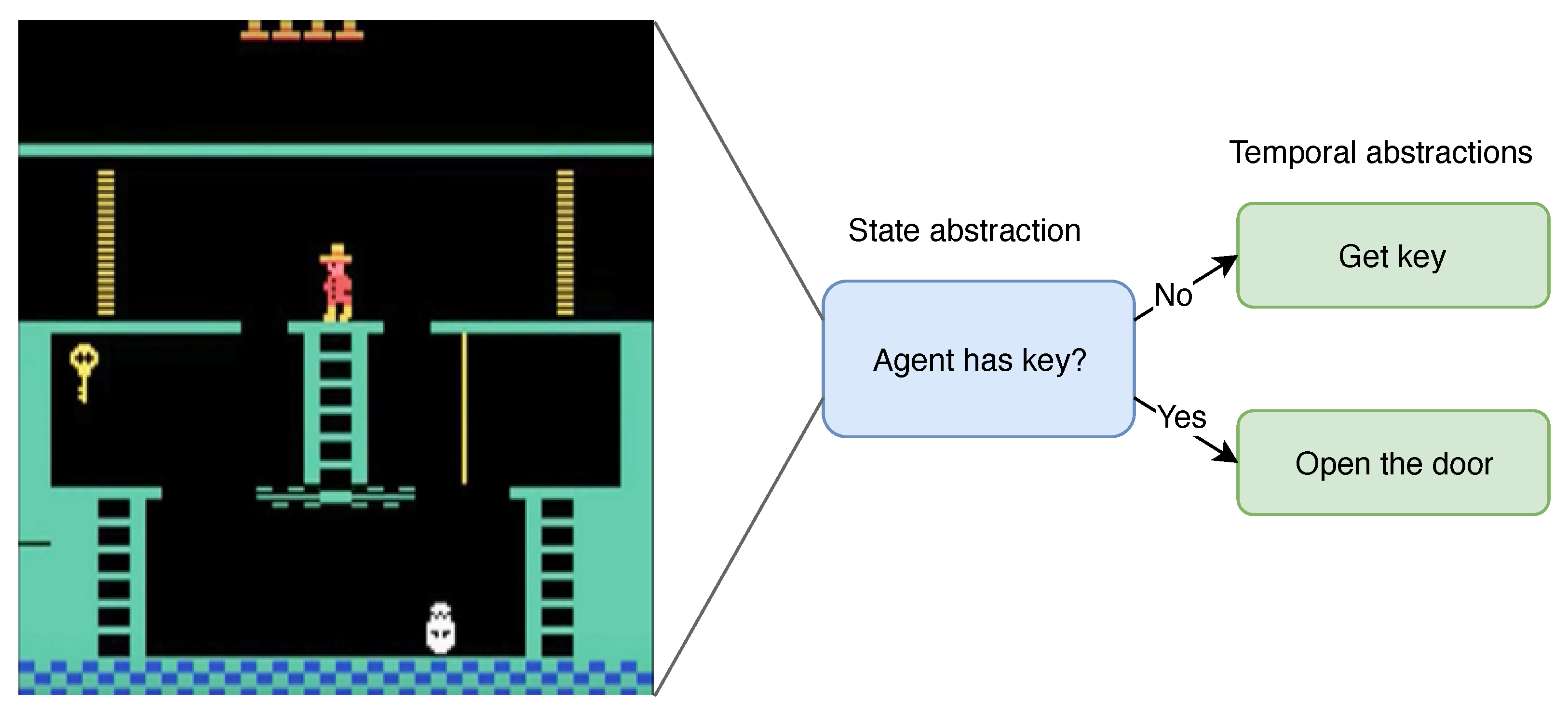
Table 1.
Summary table of the reviewed HRL frameworks.
| Problem-Specific Models | Options | Goal-Conditional | |
|---|---|---|---|
| Sub-behaviors | Problem-specific sub-behaviors that work together in order to solve a very specific task. | A more generic system of modules that work together to tackle a limited set of similar sub problems. | A generic system that is capable of expressing a wide range of sub-behaviors. |
| Capabilities | Intuitive way of modeling hierarchies of sub-behaviors. | - Generic framework capable of modeling sub-behaviors. - Transfers well in similar environments. - Various learning algorithms available. | - Generalization of sub-behaviors. - Capable of supporting a large amount of sub-behaviors. - Various learning algorithms available. |
| Challenges | - Not generally applicable. - Requires a lot of expert knowledge. - Lack of learning algorithms. | - Learning is often sample inefficient. - Difficult to share knowledge between options. - Limited scalable: only a few options at the same time are feasible. | - Efficient representation of subgoals. - How to efficiently sample goal-vectors during training, in order to maximize generalization over sub-behaviors. - Often suffers from instability. - Scaling to more than two levels remains difficult. |
| Required priors | Almost entirely hand-crafted. | Some expert knowledge required in the form of termination conditions, and intrinsic reward signals. | None, however intrinsic reward has been demonstrated to speed up training [155]. |
| Interpretability | High | High, however often due to introduced priors | Low, often uses latent-spaces. |
Table 2.
Evaluation of problem-specific algorithms.
| Algorithm | Training Method | Required Priors | Interpretable Elements | Transferrable Policy | Improvement |
|---|---|---|---|---|---|
| Feudal-Q | End-to-end | State-space division | None | No, problem-specific solution | More comprehensive exploration than flat Q-learning |
| HAM-Q | End-to-end | HAM | Trained HAMs | HAM language can be used to transfer knowledge | Significant improvement over flat Q-learning |
| MAXQ-Q | End-to-end | MAXQ decomposition | MAXQ decomposition | MAX-nodes | Faster training, compared to flat Q-learning |
| HEXQ | Staged | None | MAXQ decomposition | MAX-nodes | Automatic discovery of MAXQ decompositions |
| VISA | End-to-end | DBN model | MAXQ decomposition | MAX-nodes | More complex decomposition than HEXQ |
| HI-MAT | End-to-end | a successful trajectory | MAXQ decomposition | MAX-nodes | More compact hierarchies than VISA |
Table 3.
Evaluation of option algorithms.
| Algorithm | Training Method | Required Priors | Interpretable Elements | Transferrable Policy | Improvement |
|---|---|---|---|---|---|
| Diverse density | Staged | Number of options, successful trajectories | Subgoal states | Same environment | Automatic subgoal detection learns faster compared to using only primitive actions |
| h-DQN | Staged | Subgoals as pixel masks | Subgoals | Same environment | First HRL approach to hard-exploration in high-dimensional state-spaces |
| HiREPs | End-to-end | Number of options | None | No, problem-specific solutions | Improved performance over non-hierarchical REPS algorithm |
| STRAW | End-to-end | None | Macro-actions | No, problem-specific solutions | Improved performance in some Atari games |
| H-DRLN | Staged | Task curriculum | None | Same environment, similar tasks | Demonstrates building blocks for lifelong learning framework |
| Eigen-Options | Staged | Number of options | Subgoals | Same environment | Discovered options allow better exploration then bottleneck-based options |
| MLSH | Staged | Number of options | None | Transfer possible to tasks different from previously seen tasks | Faster training performance when applied on new tasks |
| DDO | Staged | Demonstrations | None | Solutions are task specific | Faster training in Atari RAM environments. |
| Option-Critic | End-to-end | Number of options | Termination probabilities | Same environment | First end-to-end algorithm |
Table 4.
Evaluation of goal-conditional algorithms.
| Algorithm | Training Method | Required Priors | Interpretable Elements | Transferrable Policy | Improvement |
|---|---|---|---|---|---|
| VIC | Staged | None | None | Same environment | Demonstrated capabilities of unsupervised learning in HRL |
| SNN | Staged | Proxy reward | Sub-behaviors | Same environment | Increased expressiveness and multimodality of sub-behaviors |
| FuN | End-to-end | None | None | Task-specific solutions | Significant improvement over Option-Critic |
| DIAYN | Staged | None | None | Same environment | Discovers more diverse sub-behavior than VIC |
| SAC-LSP | Staged and End-to-end | None, however reward shaping is supported | None | Same environment | Outperforms previously proposed non-hierarchical algorithms |
| HIRO | End-to-End | None | None | Same environment | Outperforms FuN, especially in sample efficiency |
| VALOR | Staged | None | None, sub-behaviors are encoded by a latent vector | Similar environments | Qualitatively better sub-behaviors than DIAYN and VIC |
Publisher’s Note: MDPI stays neutral with regard to jurisdictional claims in published maps and institutional affiliations. |
© 2022 by the authors. Licensee MDPI, Basel, Switzerland. This article is an open access article distributed under the terms and conditions of the Creative Commons Attribution (CC BY) license (https://creativecommons.org/licenses/by/4.0/).
Share and Cite
MDPI and ACS Style
Hutsebaut-Buysse, M.; Mets, K.; Latré, S. Hierarchical Reinforcement Learning: A Survey and Open Research Challenges. Mach. Learn. Knowl. Extr. 2022, 4, 172-221. https://doi.org/10.3390/make4010009
AMA Style
Hutsebaut-Buysse M, Mets K, Latré S. Hierarchical Reinforcement Learning: A Survey and Open Research Challenges. Machine Learning and Knowledge Extraction. 2022; 4(1):172-221. https://doi.org/10.3390/make4010009
Chicago/Turabian StyleHutsebaut-Buysse, Matthias, Kevin Mets, and Steven Latré. 2022. "Hierarchical Reinforcement Learning: A Survey and Open Research Challenges" Machine Learning and Knowledge Extraction 4, no. 1: 172-221. https://doi.org/10.3390/make4010009