KGEARSRG: Kernel Graph Embedding on Attributed Relational SIFT-Based Regions Graph


Information Technology Services, University of Naples “L’Orientale”, 80121 Naples, Italy
†
Current address: Via Nuova Marina, 59, 80133 Naples, Italy.
Mach. Learn. Knowl. Extr. 2019, 1(3), 962-973; https://doi.org/10.3390/make1030055
Submission received: 28 June 2019
/
Revised: 26 August 2019
/
Accepted: 27 August 2019
/
Published: 28 August 2019
(This article belongs to the Section Learning)
Abstract
:In real world applications, binary classification is often affected by imbalanced classes. In this paper, a new methodology to solve the class imbalance problem that occurs in image classification is proposed. A digital image is described through a novel vector-based representation called Kernel Graph Embedding on Attributed Relational Scale-Invariant Feature Transform-based Regions Graph (KGEARSRG). A classification stage using a procedure based on support vector machines (SVMs) is organized. Methodology is evaluated through a series of experiments performed on art painting dataset images, affected by varying imbalance percentages. Experimental results show that the proposed approach consistently outperforms the competitors.
1. Introduction
Support vector machines (SVMs) [1] have found applications in different fields such as image retrieval [2], handwriting recognition [3] and text classification [4]. In the case of imbalanced data, in which the number of negative patterns, easier to identify and classify, significantly exceeds the positive patterns, which are more difficult to identify and classify, the performance of SVM drops considerably. In general, classifiers perform poorly with imbalanced datasets because they are designed to work on sample data and the output is formulated from the simpler hypothesis that best fits the data. With imbalanced data, the simplest hypothesis is often that all patterns are classified as negative; in essence the positive patterns are not detected by the classifier, being included in the patterns classified as negative in a completely wrong way. Another important issue, which makes the classifier too specific, is sensitivity to noise, which in many cases leads to a wrong hypothesis. Specifically, some researchers modify the behavior of existing algorithms for the purpose of making them more immune to noisy instances. These approaches are designed for balanced datasets and, with highly imbalanced datasets, every pattern is classified as negative. Furthermore, the positive may be treated as noise and completely ignored by the classifier. A widely used approach is to bias the classifier to ensure more attention to the positive patterns. In this paper, the image classification problem applied to imbalanced datasets is addressed. In particular, an image is represented by a data structure Attributed Relational Scale-Invariant Feature Transform-based Regions Graph (ARSRG) [5]. This approach is used in order to capture local and structural image features. Moreover, ARSRG structures are mapped into a vector space through a graph kernel application. Graph kernels aim at bridging the gap between the high representational power and the flexibility of graphs in terms of feature vector representation. The images to be classified, also called target images, are encoded through a set of distances with model images. The final representation is called Kernel Graph Embedding on Attributed Relational Scale-Invariant Feature Transform-based Regions Graph (KGEARSRG). The classification stage is managed through SVM, using the One versus All (OvA) paradigm, with the appropriate kernel modification called Asymmetric Kernel Scaling (AKS) [6].
2. Related Work
One of the biggest challenges during the design of a classifier regards the resolution of the imbalance between the number of images belonging to a class focused by a user and the others that share some features with that class. The imbalance problem has been investigated in literature applied to the image classification field.
In [7] the authors compare the performance of artificial immune system-based image classification algorithms to the performance of Gaussian kernel-based SVM in problems with a high degree of class imbalance.
In [8] a methodology, based on resampling, developed to solve the class imbalance problem in the classification of thin-layer chromatography (TLC) images is introduced. In addition, two approaches are proposed for image classification. One based on a hierarchical classifier and another using a multiclassifier system. Both classifiers are trained and tested using balanced datasets.
In [9] an approach for building a classification system for imbalanced data based on a combination of several classifiers is presented. A final classification system combining all the single trained classifiers is built. The approach can be defined as a sort of local undersampling, since each classifier uses a part of the majority samples, or global oversampling since the minority class is replicated M times.
In [10] two genetic programming (GP) methods for image classification problems with class imbalance are developed and compared. The first works on adapting a fitness function in GP in order to evolve classifiers with good individual class accuracy, while the second implements a multi-objective approach to simultaneously evolve a set of classifiers along a trade-off surface representing minority and majority class accuracies.
In [11] a methodological approach to classification of pigmented skin lesions in dermoscopy images is presented. SVM is used for the classification step. The class imbalance problem is addressed using various sampling strategies and through Monte Carlo cross validation.
In [12] the problem of diagnosing genetic abnormalities by classifying a small image imbalanced database of fluorescence in situ hybridization signals of types having different frequencies of occurrence is addressed.
Finally, in [13] is investigated how class imbalance in the available set of training cases can impact the performance of the resulting classifier as well as properties of the selected set. The test phase is performed on a dataset for the problem of detecting breast masses in screening mammograms. Binary and k-nearest neighbor classifiers are adopted.
3. Kernel Graph Embedding on Attributed Relational SIFT-Based Regions Graph (KGEARSRG)
In this section a novel kernel graph with reference to the ARSRG structure is introduced. This representation is called Kernel Graph Embedding on Attributed Relational Scale-Invariant Feature Transform-based Regions Graph (KGEARSRG). Let be a dataset composed of N ARSRG structures in a D-dimensional space. The aim is to reduce the dataset into a low-dimensional space , such that ARSRG topological information is preserved from to . The framework attempts to find the optimal low dimensional vector representation that best characterizes the similarity relationship between the node pairs in ARSRG structures.
3.1. Graph-Based Image Representation
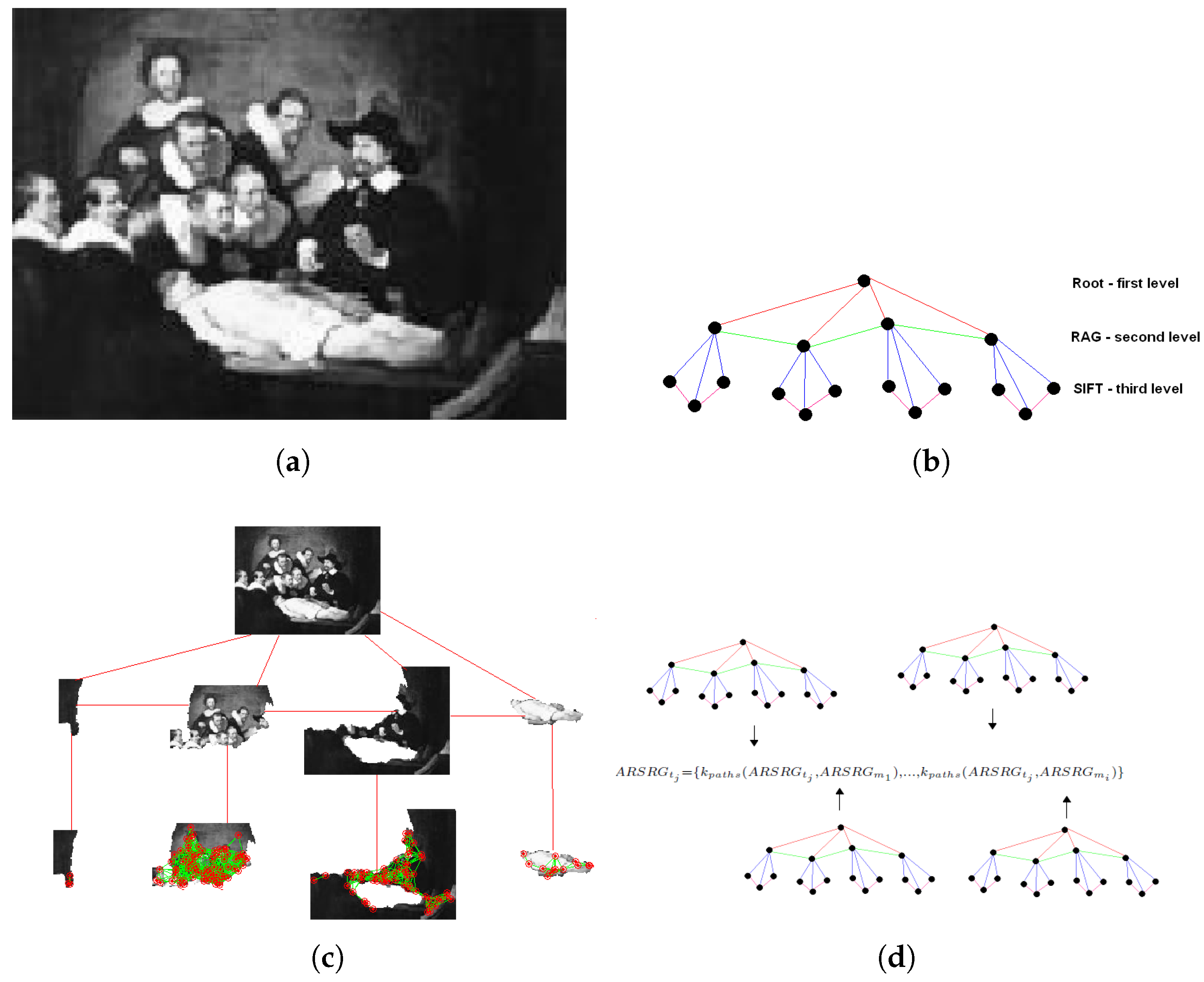
The Attributed Relational SIFT-based Regions Graph (ARSRG) [5] is adopted to represent images and is built based on two phases. The first phase, named feature extraction, provides regions of interest (ROIs) from images by means of a segmentation technique and constructs a Region Adjacency Graph (RAG) [14] to encode spatial relations between extracted regions. The second phase, named graph construction, provides the construction of a graph, named the Attributed Relational SIFT-based Regions Graph (ARSRG), formed by three levels: Root node, RAG nodes and leaf nodes. The root node encodes the whole image and is connected to all the RAG nodes at the second level. RAG nodes encode geometric information among different image regions. Thus, spatially adjacent regions in the image are represented by connected nodes. Finally, leaf nodes represent the set of SIFT [15] descriptors extracted from the image in order to ensure invariance to different conditions (view-point, illumination and scale). This level provides two types of configurations: region based, in which a keypoint is associated to a region based on its spatial coordinates, and region graph based, in which keypoints belonging to the same region are connected by edges to encode spatial information. ARSRG is created based on two different leaf nodes configurations.
3.2. Graph Embedding
The goal is to provide a fixed-dimensional vector space image representation in order to process the data for classification purposes. To this end, the concept of graph embedding is introduced. Given a labeled set of sample graphs, and the graph dissimilarity measure is . T can be any kind of graph set and can be any kind of dissimilarity measure. Subsequently, based on a selected set of prototypes from T, the dissimilarity of a given input graph g is computed to each prototype . This leads to m dissimilarities, , which can be represented in an m-dimensional vector . In this way, any graph can transformed from the training as well as any other graphs set into a vector of real numbers. More formally, given a graph domain G,
the training set of graphs, subject to the next mapping phase, and
a set of prototype graphs. The vector of mapping between T and P is defined as
where is any graph dissimilarity measure between graph g and the ith prototype. The distance does not obey the triangular inequality. Considering the graphs , , and the triangular inequality
Equation (4) is not verified as it deals with complex structures where the number of nodes and edges can be associated in a different way during the matching, and the distance varies according to the chosen metric. This is a very complex problem that cannot be generalized using the triangular inequality.
3.3. Kernel Graph Embedding
Kernel graph embedding is a framework that works with the purpose of extending the dot product space from a linear to a nonlinear case using the kernel trick. The goal is to map data from the original input space to an alternative higher dimensional space as
with being the implicit pairwise embedding between and . The concept of kernel graph embedding is applied in a particular way. Firstly, ARSRG structure extraction, from images stored in the entire dataset, is performed. After, the ARSRG set is divided into two subsets in the following way:
The first subset is composed of target images as in Equation (1), subset training T, while the second subset is composed of model images as in Equation (2), subset prototypes P. Now, the distance vector representing each ARSRG, belonging to a target set, is built as follows:
The vector components encode the distance between and all ARSRGs contained in the subset prototypes. Distance values are calculated through the kernel graph in [16] applied on ARSRG pairs, particularly
where and are the sets of all paths in and , located at the third level of structures in the form of SIFT Nearest-Neighbor Graphs (SNNGs). An SNNG is defined as follows:
where:
- is the set of nodes associated to SIFT keypoints;
- is the set of edges.
For each there is an edge if and only if . is a Euclidean distance applied to the x and y positions of keypoints in the image, is a threshold value and p stems from 1 to k, k being the size of . A path is, as usual, defined as a sequence of nodes, consisting of at least one node and without any repetitions of nodes. Defining paths as sequences of neighboring pairwise distinct edges allows to define kernels based on subpaths. In this context, edge walk and edge path are defined. Given a graph with and , an edge walk
is defined as a sequence of edges from to , where , with , is a neighbor of , i.e., and are neighbors if . An edge path p is defined as an edge walk without repetitions of the same edge. An edge path may contain the same node multiple times but every edge only once. An edge path p is an Euler path in the graph exactly consisting of the edges of p. In this case, edge paths are used. Moreover, is a positive definite kernel on two paths, defined as the product of kernels on edges and nodes along the paths. To this end, a relation is defined, where is a path and and x are graphs. if is the graph created removing all edges in from x. is then the set of all possible decompositions of the graph x via R into and . R is finite and its length is upper bounded by the number of edges, based on a finite number of paths in the graph. Now, a kernel on paths is defined as a product of kernels on nodes and edges in these paths, also named tensor product kernel. Moreover, a trivial graph kernel is defined for all pairs of graphs. Now, an all-paths kernel is defined as a positive definite R-convolution as
where and are the sets of all paths in and . In this case, kernel graph application requires a preprocessing step. ARSRGs are compared through the algorithm in [5], which provides SNNG pairs for the final application of the kernel graph. Essentially, edge path search is performed on graphs contained in the ARSRG regions. Based on this procedure, , in Equation (8), encodes the distance between SNNG pairs belonging to regions in the matching set. Finally, kernel matrix K may be expressed as:
More precisely, given the sets and in the equations, matrix K encodes all pairwise distances between the ARSRGs. In particular, each row of the matrix K corresponds to a vector-based representation of as in Equation (7). This demonstrates how the vector-based representation can be adopted for kernel matrix K and, subsequently, in the classification of ARSRG structures. Figure 1 shows an example of an image represented by KGEARSRG.
Computational Cost
The computational cost related to KGEARSRG can be divided into different parts:
- The computational cost for extracting SNNG pairs between image regions through SIFT match with graph matching.
- Kernel graph computation involves:
- (a)
- The direct product graph upper bounded by , where n is the number of nodes.
- (b)
- The inversion of the adjacency matrix of this direct product graph; standard algorithms for the inversion of an matrix require time.
- (c)
- The shortest-path kernel requires a Floyd-transformation algorithm which can be performed in time. The number of edges in the transformed graph is when the original graph is connected. Pairwise comparison of all edges in both transformed graphs is required to determine the kernel value. pairs of edges are considered, which results in a total runtime of .
4. Experimental Results
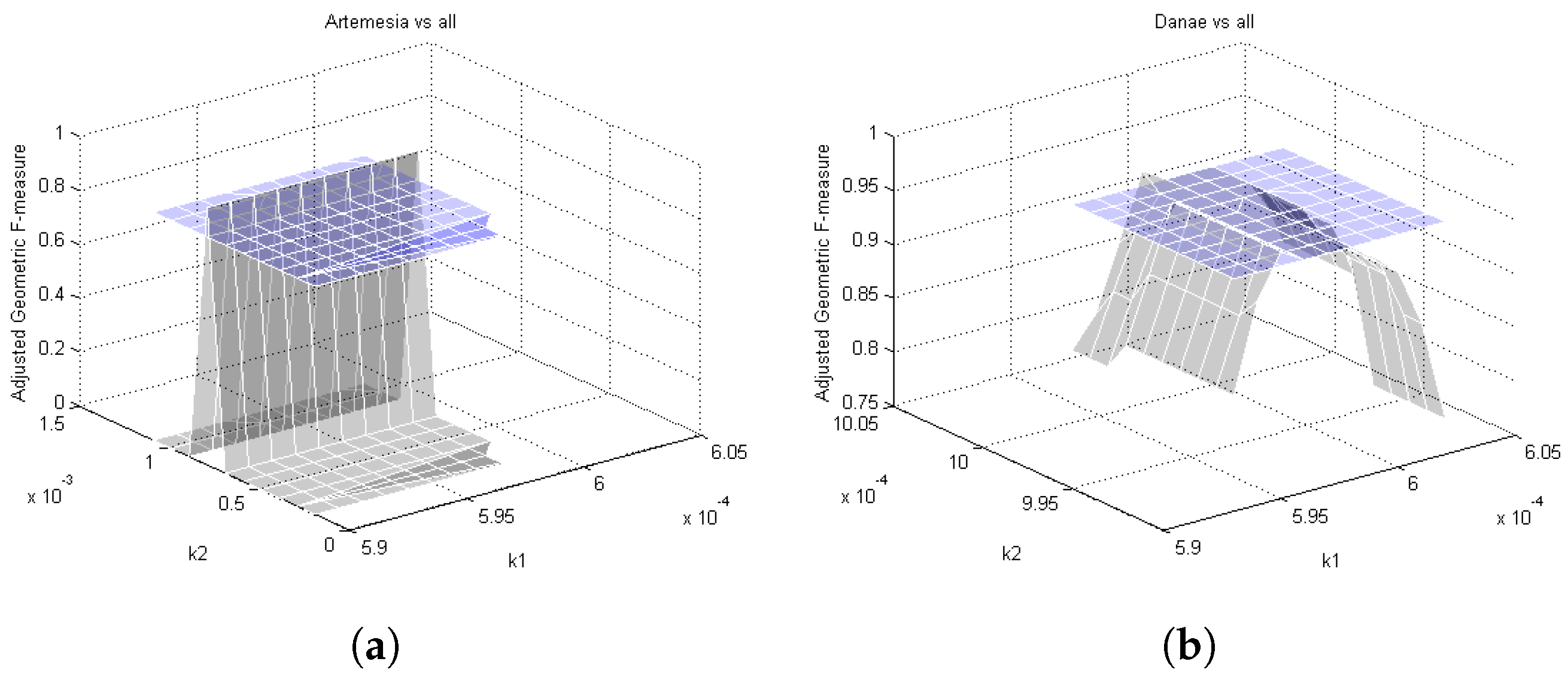
The proposed algorithm has been applied to the art painting classification problem [17]. The datasets adopted are publicly available and contain different digitized images of paintings together with the corresponding ground truth data. The testing phase is organized into different blocks. First a comparison with standard SVM [1] is performed. The second phase, differently, involves a comparison with C4.5 [18], RIPPER [19], L2 Loss SVM [20], L2 Regularized Logistic Regression [21] and ripple-down rule learner (RDR) [22]. Finally, performances are evaluated in terms of Adjusted F-measure (AGF) [6]. With reference to Equation (9), it is important to focus attention on two parameters. allows to connect two SIFT keypoints and is estimated based on the density and spatial proximity of keypoints. Clearly, the spatial proximity leads to a reduction of the value. k represents the number of SIFT keypoints, the size of , to be analyzed in order to construct the SNNG. Moreover, during classification, with reference to Equation (14), the values and are used to transform the kernel and are connected to the size of the input data of each class. The range adopted is variable, as they are very sensitive parameters, and can be easily understood through the x and y axes of the graphs in Figure 2 and Figure 3.
The framework has been developed in two different programming languages. The kernel was developed in Matlab code, while the part related to classification was developed in Java code, with integration in Waikato Environment for Knowledge Analysis (WEKA) (https://www.cs.waikato.ac.nz/ml/weka/).
4.1. Asymmetric Kernel Scaling (AKS) for Support Vector Machines
The main idea, to preserve local angles, consists in applying a conformal transformation. In [23], with purpose of improving SVM performance, a (quasi) conformal transformation on the kernel is adopted. The aim is to increase the break up between the two classes near the boundary and therefore to widen the resolution in this area. The general transformation form is:
where positive is defined. is Gaussian, and meets Mercer conditions, if and K are Gaussian.
The improvement consists in managing various training instances in the two classes [6]. The goal is to extend areas located near the sides of the separation, which represent the boundary on the surface, in order to compensate for its asymmetry related to minority instances. In the first instance, SVM provides an approximate boundary position. Subsequently, the negative and the positive points are segmented into two sets. In the second instance, the following kernel transformation is applied:
where and are free parameters and is given by:
The instance class relies on the location of the hyperplane where it falls, specifically with rerefence to the sign of . Support Vectors (SVs) are by definition the such that and b represents the bias; by doing this, the space is enlarged on different sides of the boundary surface, which makes it possible to equilibrate the imbalance due to the data. Proper values for and are adopted to manage the transformed kernel during classification and are estimated based on the size of the input data of each class.
4.2. OvA Classification Setting
The classification performance of the AKS classifier is tested over the standard OvA paradigm on different low, medium and high imbalanced image classification problems. One of the simplest multiclass classification schemes is to create N different binary classifiers, each one trained in order to distinguish the pattern of a single class among the patterns in remaining classes. When a new pattern is ready for classification, the N classifiers are run and the classifier that outputs the largest positive value is chosen. In the case shown, a skewed dataset is considered, where a positive minority class of patterns has to be recognized against a negative majority class. At this point, the application of the OvA schema is simple; each image of a target set, encoded by the KGEARSRG procedure, is submitted to the classification process; then the membership class associated to this image is considered against others present in the target set. This step is performed for all membership classes with the purpose of compensating the multiclass case.
4.3. Datasets
The first dataset [24] is composed of two sets of images belonging to 16 classes. The first set contains 15 paintings belonging to Olga’s gallery (http://www.abcgallery.com/index.html) and is named the originals set. The second set contains 100 photos of paintings, taken by tourists with different digital cameras, available on Travel Webshots (http://travel.webshots.com) and is named the photographs set. We adopt the originals set as the model set and the photographs set as the target set, with images to be classified. The second dataset [5] is composed of 99 painting photos taken from the Cantor Arts Center (http://museum.stanford.edu/). The images are divided into 33 classes. In addition, in order to apply image classification tasks, 10 additional images, belonging to 33 classes, have been added. We adopt the first 99 painting photos as the model set and the last 10 additional images as the target set, the images to be classified. Subsequently, the imbalance rates to formulate different classification problems are calculated. Table 1 and Table 2 show settings about the configuration of the datasets and, in particular, the imbalance rate (IR) in the last column is shown with reference to Equation (16).
IR is defined as the ratio between the percentage of images belonging to the majority class over the minority class.
4.4. AKS vs. SVM
This section describes the comparison between AKS and SVM. The experiments are conducted by performing, in the first instance, a standard SVM classification, using a Gaussian kernel with base 0.5 and , tuned through a grid search. Subsequently, the two step AKS described above is applied. In the second step of AKS, the classification with the transformed kernel is performed. Grid search and fivefold cross validation have been applied to find the optimal value of the parameters and AGF has been used as the performance measure.
It can be seen in Figure 2 that the proposed method needs a wide search in the parameters space for fine tuning and the performance is shown to be very sensitive to a good choice of parameters. Out of a narrow interval of and for effective improvement, performance tends to drop quickly. Comparing performance with a careful choice of parameters, the proposed approach consistently dominates standard SVM. Differently, in Figure 3 performances are higher only with a single peak with respect to standard SVM.
4.5. Comparison Results
Further tests have been conducted in order to perform a comparison with C4.5 [18], RIPPER [19], L2 Loss SVM [20], L2 Regularized Logistic Regression [21] and ripple-down rule learner (RDR) [22] for a complete set of OvA classification problems. The parameters of the competitors are submitted to a tuning procedure using a very wide range with respect to the parameters of the proposed method and are subsequently initialized randomly. The best performances are shown below. The results of the two datasets are different due to imbalance rates. In the dataset in [24], configuration includes approximately low, medium and high rates. It is a great dataset for a robust testing phase because it covers full cases of class imbalance problems. In the dataset in [5], imbalance rates are identical for all configurations. The behavior of classifiers can be analyzed through Table 3 and Table 4. Table 3 shows the results of the dataset in [24]. It can be seen that performances are significantly higher than in the comparison methods. The improvement provided by AKS lies in the accuracy of the classification of patterns belonging to the minority class, positive, which, during the relevance feedback evaluation, have a greater weight. Indeed, these latter are difficult to classify compared to patterns belonging to the majority class, negative. The results reach a high level of correct classification. This indicates that the improvements over existing techniques can be associated with two aspects. The first involves the vector-based image representation extracted through KGEARSRG. The second concerns the use of the AKS method for the classification stage. Table 4, in the same as previous the way, shows the improvement introduced by AKS. Finally, for both cases results indicate that the classification performance of AKS on the minority class is significantly higher than the corresponding performance of the others classifiers. It is clear that our approach has the intrinsic ability to more efficiently address classification problems that are extremely imbalanced. In other words, the AKS classifier retains the ability to correctly recognize patterns originating from the minority class compared to the majority class.
5. Conclusions
Data imbalance classification is a common challenge in many fields such as pattern recognition, bioinformatics and data mining. In this paper, the imbalance problem in image classification is addressed. A novel way to represent a digital image based on KGEARSRG is presented. This representation is proved to be very useful for mapping a dense graph space to a reduced space. The classification task is managed through the SVM method based on a transformed kernel, named AKS. Experimental results indicate that the combined approach of KGEARSRG and AKS has the intrinsic property of dealing more efficiently with highly imbalanced datasets. Specifically, the method identifies instances from the minority class more efficiently as compared to other classifiers in the same domain. In future, we will provide a comparison against MLPs, k-NN and a mixture of models for different classification problems having a serious degree of class imbalance.
Funding
This research received no external funding.
Acknowledgments
This work is dedicated to Alfredo Petrosino. With him I took my first steps in the field of computer science. During these years spent together, I learned firmness in achieving goals, love and passion for the work. I will be forever grateful. Thank you my great master.
Conflicts of Interest
The author declares no conflict of interest.
References
- Vapnik, V. Statistical Learning Theory; John Wiley and Sons: New York, NY, USA, 1998. [Google Scholar]
- Lan, T.; Yang, W.; Wang, Y.; Mori, G. Image retrieval with structured object queries using latent ranking SVM. In Proceedings of the European Conference Computer Vision, Florence, Italy, 7–13 October 2012; pp. 129–142. [Google Scholar]
- Hajj, N.; Awad, M. Isolated handwriting recognition via multi-stage Support Vector Machines. In Proceedings of the International Conference in Intelligent Systems, Sofia, Bulgaria, 6–8 September 2012; pp. 152–157. [Google Scholar]
- Ji, L.; Cheng, X.; Kang, L.; Li, D.; Li, D.; Wang, K.; Chen, Y. A SVM-Based Text Classification System for Knowledge Organization Method of Crop Cultivation. In Computer and Computing Technologies in Agriculture V; Springer: Berlin/Heidelberg, Germany, 2012; pp. 318–324. [Google Scholar] [Green Version]
- Manzo, M.; Petrosino, A. Attributed Relational Sift-based Regions Graph for art painting retrieval. In Proceedings of the ICIAP 2013, Naples, Italy, 9–13 September 2013; pp. 833–842. [Google Scholar]
- Maratea, A.; Petrosino, A.; Manzo, M. Adjusted F-measure and Kernel Scaling for Imbalanced Data Learning. Inf. Sci. 2014, 257, 331–341. [Google Scholar] [CrossRef]
- Sotiropoulos, D.N.; Tsihrintzis, G.A. Artificial Immune System-based Classification in Class-Imbalanced Image Classification Problems. In Proceedings of the 2012 Eighth International Conference on Intelligent Information Hiding and Multimedia Signal Processing, Piraeus-Athens, Greece, 18–20 July 2012; pp. 138–141. [Google Scholar]
- Sousa, A.; Mendonça, A.; Campilho, A. The class imbalance problem in TLC image classification. In Proceedings of the Image Analysis and Recognition, Póvoa de Varzim, Portugal, 18–20 September 2006; pp. 513–523. [Google Scholar]
- Molinara, M.; Ricamato, M.T.; Tortorella, F. Facing imbalanced classes through aggregation of classifiers. In Proceedings of the International Conference on Image Analysis and Processing, Modena, Italy, 10–14 September 2007; pp. 43–48. [Google Scholar]
- Bhowan, U.; Zhang, M.; Johnston, M. Genetic programming for image classification with unbalanced data. In Proceedings of the International Conference of Image and Vision Computing New Zealand, Wellington, New Zealand, 23–25 November 2009; pp. 316–321. [Google Scholar]
- Celebi, M.E.; Kingravi, H.A.; Uddin, B.; Iyatomi, H.; Aslandogan, Y.A.; Stoecker, W.V.; Moss, R.H. A methodological approach to the classification of dermoscopy images. Comput. Med. Imaging Graph. 2007, 31, 362–373. [Google Scholar] [CrossRef] [PubMed] [Green Version]
- Lerner, B.; Yeshaya, J.; Koushnir, L. On the classification of a small imbalanced cytogenetic image database. Trans. Comput. Bioinform. 2007, 4, 204–215. [Google Scholar] [CrossRef] [PubMed]
- Malof, M.; Mazurowski, M.A.; Tourassi, G.D. The effect of class imbalance on case selection for case-based classifiers: An empirical study in the context of medical decision support. Neural Netw. 2012, 25, 141–145. [Google Scholar] [CrossRef] [PubMed] [Green Version]
- Tremeau, A.; Colantoni, P. Regions adjacency graph applied to color image segmentation. Trans. Image Process. 2000, 9, 735–744. [Google Scholar] [CrossRef] [PubMed]
- Lowe, D.G. Distinctive image features from scale-invariant keypoints. Int. J. Comput. Vis. 2004, 60, 91–110. [Google Scholar] [CrossRef]
- Borgwardt, K.M.; Kriegel, H.P. Shortest-path kernels on graphs. In Proceedings of the Fifth IEEE International Conference on Data Mining (ICDM’05), Houston, TX, USA, 27–30 November 2005; pp. 74–81. [Google Scholar]
- Culjak, M.; Mikus, B.; Jez, K.; Hadjic, S. Classification of art paintings by genre. In Proceedings of the MIPRO 34th International Convention, Opatija, Croatia, 23–27 May 2011; pp. 1634–1639. [Google Scholar]
- Quinlan, J.R. C4.5: Programs for Machine Learning; Morgan Kaufmann Publishers: San Mateo, CA, USA, 1993. [Google Scholar]
- Cohen, W.W. Fast effective rule induction. In Proceedings of the 12th International Conference in Machine Learning, Tahoe City, CA, USA, 9–12 July 1995; Morgan Kaufmann: San Mateo, CA, USA, 1995; pp. 115–123. [Google Scholar]
- Boser, B.E.; Guyon, I.M.; Vapnik, V.N. A training algorithm for optimal margin classifiers. In Proceedings of the 5th Annual Workshop on Computational Learning Theory, Pittsburgh, PA, USA, 27–29 July 1992; pp. 144–152. [Google Scholar]
- Fan, R.E.; Chang, K.W.; Hsieh, C.J.; Wang, X.R.; Lin, C.J. LIBLINEAR: A library for large linear classification. J. Mach. Learn. Res. 2008, 9, 1871–1874. [Google Scholar]
- Dazeley, R.; Warner, P.; Johnson, S.; Vamplew, P. The Ballarat Incremental Knowledge Engine. In Proceedings of the 11th International Workshop on Knowledge Management and Acquisition for Smart Systems and Services, Daegue, Korea, 20 August–3 September 2010; pp. 195–207. [Google Scholar]
- Amari, S.; Wu, S. Improving svm classifiers by modifying kernel functions. Neural Netw. 1999, 12, 783–789. [Google Scholar] [CrossRef]
- Haladová, Z.; Šikudová, E. Limitations of the SIFT/SURF based methods in the classifications of fine art paintings. Internet J. Comput. Graph. Geom. 2010, 12, 40–50. [Google Scholar]
Figure 1.
Example of Kernel Graph Embedding on Attributed Relational SIFT-based Regions Graph (KGEARSRG) application. (a) Original image; (b) Attributed Relational SIFT-based Regions Graph (ARSRG) structure; (c) original image represented by ARSRG structure; (d) vector representation based on KGEARSRG.

Figure 2.
Parameter choice 1. The x and y axes represent the values of the parameters of the two methods, while on the z axis is plotted the AGF for two of the OvA configurations of the dataset in [24]: (a) Artemisia vs. all and (b) Danae vs. all. The gray and blue surfaces represent, respectively, the results with the AKS and SVM classifiers.

Figure 3.
Parameter choice 2. The x and y axes represent the values of the parameters of the two methods, while on the z axis is plotted the AGF for two of the OvA configurations on the dataset in [5]: (a) Class 4 vs. all and (b) class 19 vs. all. The gray and blue surfaces represent, respectively, the results with the AKS and SVM classifiers.


Table 1.
The one vs. all (OvA) configuration for the dataset in [24].
Table 1.
The one vs. all (OvA) configuration for the dataset in [24].
| Problem | Classification Problem | (%min,%maj) | IR |
|---|---|---|---|
| 1 | Artemisia vs. all | (3.00,97.00) | 32.33 |
| 2 | Bathsheba vs. all | (3.00,97.00) | 32.33 |
| 3 | Danae vs. all | (12.00,88.00) | 7.33 |
| 4 | Doctor_Nicolaes vs. all | (3.00,97.00) | 32.33 |
| 5 | HollyFamilly vs. all | (2.00,98.00) | 49.00 |
| 6 | PortraitOfMariaTrip vs. all | (3.00,97.00) | 32.33 |
| 7 | PortraitOfSaskia vs. all | (1.00,99.00) | 99.00 |
| 8 | RembrandtXXPortrai vs. all | (2.00,98.00) | 49.00 |
| 9 | SaskiaAsFlora vs. all | (3.00,97.00) | 32.33 |
| 10 | SelfportraitAsStPaul vs. all | (8.00,92.00) | 11.50 |
| 11 | TheJewishBride vs. all | (4.00,96.00) | 24.00 |
| 12 | TheNightWatch vs. all | (9.00,91.00) | 10.11 |
| 13 | TheProphetJeremiah vs all | (7.00,93.00) | 13.28 |
| 14 | TheReturnOfTheProdigalSon vs. all | (9.00,91.00) | 10.11 |
| 15 | TheSyndicsoftheClothmakersGuild vs. all | (5.00,95.00) | 19.00 |
| 16 | Other vs. all | (26.00,74.00) | 2.84 |
Table 2.
The OvA configuration for the dataset in [5].
Table 2.
The OvA configuration for the dataset in [5].
| Problem | Classification Problem | (%min,%maj) | IR |
|---|---|---|---|
| 1 | Class 4 vs. all | (1.00,9.00) | 9.00 |
| 2 | Class 7 vs. all | (1.00,9.00) | 9.00 |
| 3 | Class 8 vs. all | (1.00,9.00) | 9.00 |
| 4 | Class 13 vs. all | (1.00,9.00) | 9.00 |
| 5 | Class 15 vs. all | (1.00,9.00) | 9.00 |
| 6 | Class 19 vs. all | (1.00,9.00) | 9.00 |
| 7 | Class 21 vs. all | (1.00,9.00) | 9.00 |
| 8 | Class 27 vs. all | (1.00,9.00) | 9.00 |
| 9 | Class 30 vs. all | (1.00,9.00) | 9.00 |
| 10 | Class 33 vs. all | (1.00,9.00) | 9.00 |
| AGF | ||||||
|---|---|---|---|---|---|---|
| Problem | AKS | C4.5 | RIPPER | L2-L SVM | L2 RLR | RDR |
| 1 | 0.9414 | 0.5614 | 0.8234 | 0.6500 | 0.5456 | 0.8987 |
| 2 | 0.9356 | 0.8256 | 0.6600 | 0.8356 | 0.8078 | 0.7245 |
| 3 | 0.9678 | 0.8462 | 0.8651 | 0.4909 | 0.6123 | 0.7654 |
| 4 | 0.9746 | 0.8083 | 0.6600 | 0.4790 | 0.4104 | 0.6693 |
| 5 | 0.9654 | 0.7129 | 0.9861 | 0.8456 | 0.4432 | 0.6134 |
| 6 | 0.9342 | 0.5714 | 0.9525 | 0.8434 | 0.9525 | 0.5554 |
| 7 | 0.9567 | 0.6151 | 0.7423 | 0.5357 | 0.4799 | 0.6151 |
| 8 | 0.8345 | 0.4123 | 0.3563 | 0.7431 | 0.5124 | 0.7124 |
| 9 | 0.9435 | 0.9456 | 0.9456 | 0.8345 | 0.6600 | 0.6600 |
| 10 | 0.8456 | 0.4839 | 0.5345 | 0.4123 | 0.4009 | 0.5456 |
| 11 | 0.9457 | 0.9167 | 0.9088 | 0.9220 | 0.8666 | 0.9132 |
| 12 | 0.6028 | 0.5875 | 0.5239 | 0.4124 | 0.4934 | 0.5234 |
| 13 | 0.8847 | 0.7357 | 0.6836 | 0.7436 | 0.7013 | 0.5712 |
| 14 | 0.9376 | 0.9376 | 0.8562 | 0.8945 | 0.8722 | 0.8320 |
| 15 | 0.9765 | 0.8630 | 0.8897 | 0.8225 | 0.7440 | 0.8630 |
| 16 | 0.7142 | 0.5833 | 0.3893 | 0.4323 | 0.5455 | 0.5111 |
| AGF | ||||||
|---|---|---|---|---|---|---|
| Problem | AKS | C4.5 | RIPPER | L2-L SVM | L2 RLR | RDR |
| 1 | 0.9822 | 0.6967 | 0.5122 | 0.4232 | 0.4322 | 0.6121 |
| 2 | 0.9143 | 0.5132 | 0.4323 | 0.4121 | 0.4212 | 0.5323 |
| 3 | 0.9641 | 0.4121 | 0.4211 | 0.4213 | 0.3221 | 0.4323 |
| 4 | 0.9454 | 0.4332 | 0.1888 | 0.4583 | 0.3810 | 0.3810 |
| 5 | 0.9554 | 0.3810 | 0.2575 | 0.5595 | 0.3162 | 0.6967 |
| 6 | 0.9624 | 0.3001 | 0.1888 | 0.1312 | 0.3456 | 0.3121 |
| 7 | 0.9344 | 0.3810 | 0.5566 | 0.4122 | 0.4455 | 0.2234 |
| 8 | 0.9225 | 0.4333 | 0.1112 | 0.2575 | 0.1888 | 0.1888 |
| 9 | 0.9443 | 0.6322 | 0.1888 | 0.1888 | 0.6122 | 0.6641 |
| 10 | 0.9653 | 0.1897 | 0.5234 | 0.6956 | 0.1888 | 0.1121 |
© 2019 by the author. Licensee MDPI, Basel, Switzerland. This article is an open access article distributed under the terms and conditions of the Creative Commons Attribution (CC BY) license (http://creativecommons.org/licenses/by/4.0/).
Share and Cite
MDPI and ACS Style
Manzo, M. KGEARSRG: Kernel Graph Embedding on Attributed Relational SIFT-Based Regions Graph. Mach. Learn. Knowl. Extr. 2019, 1, 962-973. https://doi.org/10.3390/make1030055
AMA Style
Manzo M. KGEARSRG: Kernel Graph Embedding on Attributed Relational SIFT-Based Regions Graph. Machine Learning and Knowledge Extraction. 2019; 1(3):962-973. https://doi.org/10.3390/make1030055
Chicago/Turabian StyleManzo, Mario. 2019. "KGEARSRG: Kernel Graph Embedding on Attributed Relational SIFT-Based Regions Graph" Machine Learning and Knowledge Extraction 1, no. 3: 962-973. https://doi.org/10.3390/make1030055