A Systematic Literature Review of Cutting Tool Wear Monitoring in Turning by Using Artificial Intelligence Techniques

Abstract

In turning operations, the wear of cutting tools is inevitable. As workpieces produced with worn tools may fail to meet specifications, the machining industries focus on replacement policies that mitigate the risk of losses due to scrap. Several strategies, from empiric laws to more advanced statistical models, have been proposed in the literature. More recently, many monitoring systems based on Artificial Intelligence (AI) techniques have been developed. Due to the scope of different artificial intelligence approaches, having a holistic view of the state of the art on this subject is complex, in part due to a lack of recent comprehensive reviews. This literature review therefore presents 20 years of literature on this subject obtained following a Systematic Literature Review (SLR) methodology. This SLR aims to answer the following research question: “How is the AI used in the framework of monitoring/predicting the condition of tools in stable turning condition?” To answer this research question, the “Scopus” database was consulted in order to gather relevant publications published between 1 January 2000 and 1 January 2021. The systematic approach yielded 8426 articles among which 102 correspond to the inclusion and exclusion criteria which limit the application of AI to stable turning operation and online prediction. A bibliometric analysis performed on these articles highlighted the growing interest of this subject in the recent years. A more in-depth analysis of the articles is also presented, mainly focusing on six AI techniques that are highly represented in the literature: Artificial Neural Network (ANN), fuzzy logic, Support Vector Machine (SVM), Self-Organizing Map (SOM), Hidden Markov Model (HMM), and Convolutional Neural Network (CNN). For each technique, the trends in the inputs, pre-processing techniques, and outputs of the AI are presented. The trends highlight the early and continuous importance of ANN, and the emerging interest of CNN for tool condition monitoring. The lack of common benchmark database for evaluating models performance does not allow clear comparisons of technique performance.

1. Introduction

Cutting tools endure mechanical, thermal, and chemical conditions that induce wear, most importantly located on their flank face (flank wear) under nominal machining conditions. The workpieces produced with worn tools may exhibit poor quality, consisting of dimensional discrepancies, poor surface roughness and residual stresses that fall out of specifications. In order to limit downtime and risks for the machine and for the production quality, the cutting tools must be replaced in a timely manner [1]. Due to several wear mechanisms occurring simultaneously [2], the evolution of tool degradation is extremely variable even at steady cutting parameters, inducing the need for detection or prediction of wear. The continuous nature of the machining process does not allow direct measurement of the tool wear degradation. Furthermore, the evolution of different condition monitoring parameters with wear differs highly depending on the measured variable, which makes tool wear estimate extremely complex [3]. In consequence, it is estimated that only 50% to 80% of numerical control machining tool life is rationally used [4], hence important waste and losses. The industrial practice occasionally contributes to this trend, by using lower cutting parameter values in order to slow the wear process and replace the tool in time [5]. Therefore, the tool life estimate is a recurring research in machining, and several approaches have been attempted, from early empiric laws [6] to stochastic modeling [7], to more advanced statistical models such as the Proportional Hazards model [8], and in recent years, Artificial Intelligence (AI) methods.

With the rise of industry 4.0, the amount of monitoring data available for analysis increases, along with the capability of automation for industrial processes, including machining [9]. An increasing number of sensors are included in machine tools, accounting for the rise in data available, but also to the variety of variables being monitored. In this context, AI can be used in order to predict the state of tool wear based on sensors data in order to replace the cutting insert before adverse effects on production are met. Contrary to previous methods, AI also provides the capability of taking into account large data sets and continuous measurements of several sensors allows updated condition monitoring.

In a 2002 review of Artificial Neural Networks (ANN) used in tool wear monitoring in turning, Bernhard Sick covered the research of the previous decade [10]. Its long conclusions summarize the state of the art at the time, but remain specific to ANN, few applications of other techniques to tool wear monitoring existing at that time. Indeed, the AI techniques evolve rapidly and the last twenty years provided a large array of models with various input and output variables, which raised numerous methodological questions. In 2010, Abellan-Nebot and Romero Subirón [11] highlighted the lack of common methodologies for the development of AI in this framework and proposed guidelines for future experiments, regardless of the machining process, using Taguchi’s orthogonal arrays [11]. In a major review of 2013, Siddhpura and Paurobally [12] comprehensively reviewed the available variables for condition monitoring and the AI techniques for decision-making in turning [12]. More recently, taking into account the recent developments in deep learning techniques, Serin et al. [13] reviewed specifically the applications of deep learning to tool wear monitoring in machining [13]. In parallel, and specifically for milling, Mohanraj et al. [14] produced a short review on the tool condition monitoring techniques in milling, highlighting the main condition monitoring variables and summarizing the AI techniques used in decision-making relative to this process, highlighting the variety of techniques available and importance of feature extraction [14]. However, despite these reviews, which are either outdated or specific to a restricted portion of AI techniques, there is a lack of hindsight on the current variety of AI techniques applied to tool life estimate in turning, their inputs, pre-processing, and outputs.

In this paper, a brief overview of the background of tool wear in turning and AI techniques is presented in Section 2. Then, in Section 3, the standardized methodology of the systematic literature review is presented and applied to the current review [15]. For this analysis, research questions are identified, then the search process is described. In Section 4, a first bibliometric analysis is performed, then an in-depth analysis of the identified literature entries is proposed in Section 5. The results are discussed in Section 6 and formal answers to the research questions are formulated in Section 7. Finally, conclusions on each aspect of the review and perspectives on future research objectives are identified in Section 8.

2. Background in Turning Process and Artificial Intelligence

This section defines some important concepts that are used through this systematic literature review. First, the concept of tool wear in turning is presented, followed by the introduction of machine learning. This section does not constitute an exhaustive description of the subjects that it describes, but rather constitutes a comprehensive introduction to the specificities of tool wear and the AI techniques discussed in the following sections. A short introduction to some of the most used AI techniques used in this systematic literature review is presented in the appendices of this article (Appendix B.1, Appendix B.2, Appendix B.3, Appendix B.4, Appendix B.5 and Appendix B.6).

2.1. Tool Wear in Single Point Turning

Any machining operation induces tool wear. The causes of degradation of the tool can be numerous and of very varied origins. Among them, the main causes of degradation are adhesion, abrasion, tribochemical reactions and surface disruption [16]. The word “wear” groups together the surface interactions leading to all of these degradation mechanisms. The predominance of one mechanism over another depends on the cutting conditions and materials. In nominal cutting conditions, the main mechanism of wear is abrasive wear resulting in the degradation of the flank face. This type of wear is favoured by the tool manufacturers, as it is considered as the steadiest and most predictable [17,18]. Prominence of other kinds of wear generally comes from poor cutting parameters choice [8]. In turning, the main cutting parameters are: cutting speed, feed rate, and depth of cut. The workpiece material and the choice of cutting parameters each have an effect on the tool life.

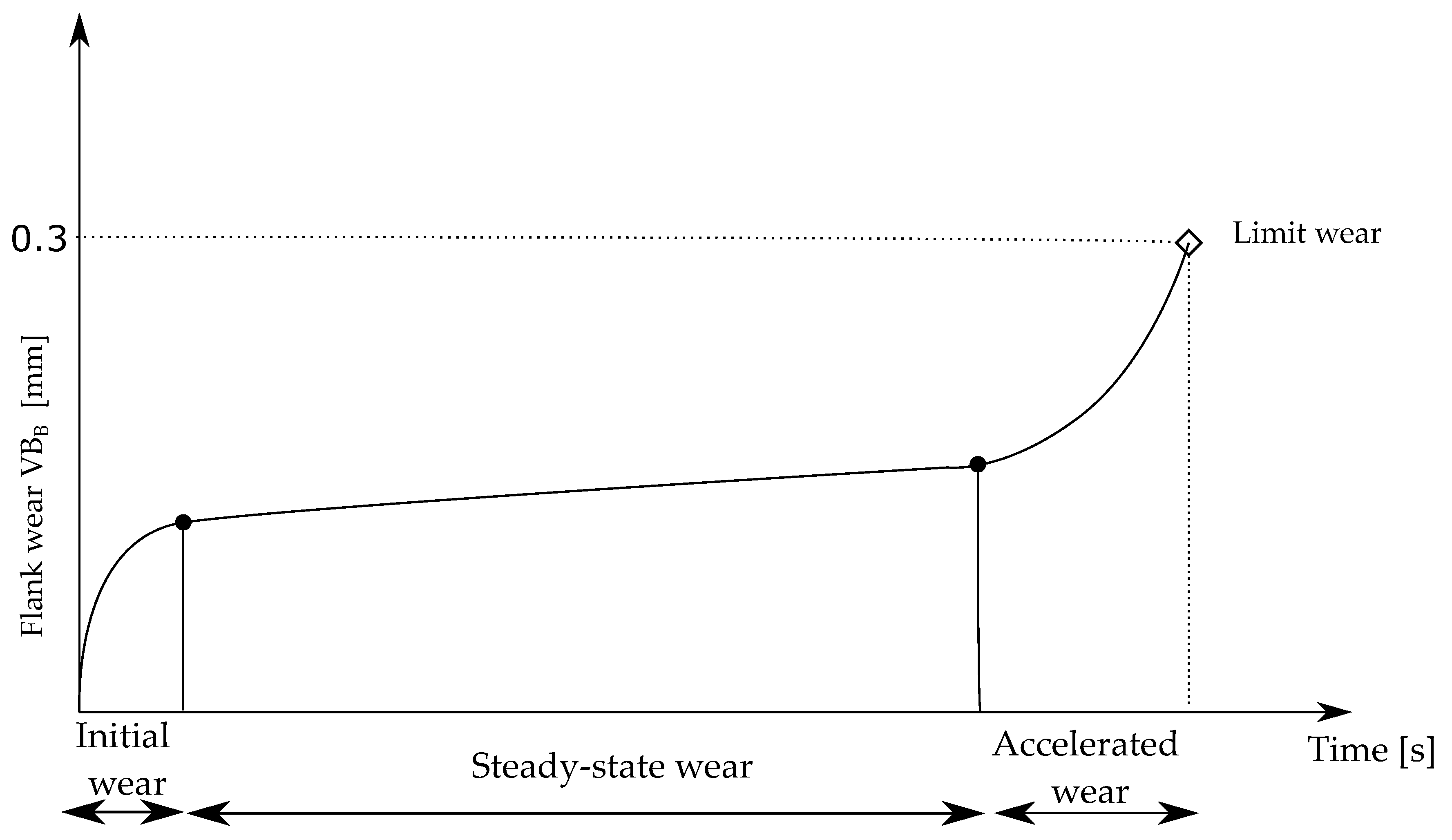
In the case of flank wear, the evolution of wear depends on the cutting condition and is constituted of three phrases (Figure 1):

• An initial wear zone. In this phase, the new insert starts to wear quickly. This period is generally short in regard of the cutting life;
• A steady-state region. In this region, the wear slowly gradually increases. The tool spends most of its life in this phase;
• Accelerated wear. This is the end-of-life of the cutting tool, the wear rate starts to increase significantly until the tool is worn. When the tool end-of-life criterion is reached, the tool is replaced by a new one.

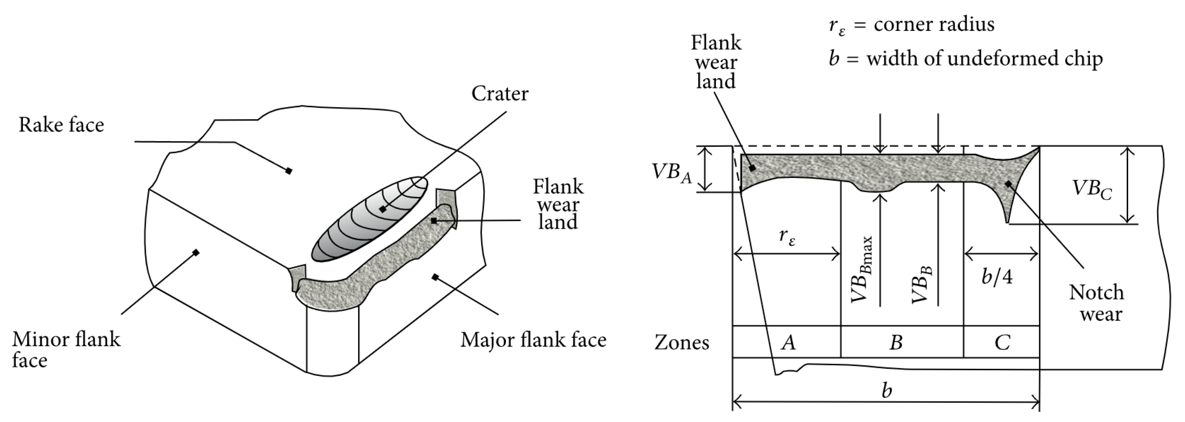
Defining an end-of-life criterion for a tool can be complex. Wear is generally accompanied by a degradation in the quality of the machined surface and compliance with required tolerances. The end-of-life criterion is thus variable, depending on the objective of the machining process. The ISO 3685 standard defines the value of ${\mathrm{VB}}_B$ as the end-of-life criterion for flank wear in the framework of single point turning tool life testing [19]. ${\mathrm{VB}}_B$ is defined as presented in Figure 2, and a tool is considered worn if the value of ${\mathrm{VB}}_B$ reaches 0.3 mm or ${\mathrm{VB}}_{B\max }$ is above 0.6 mm. In industrial applications, this criterion may vary depending on the machining purpose. The value of ${\mathrm{VB}}_B$ is obtained by directly measuring the wear land width on the flank face (Figure 2).

2.2. Artificial Intelligence

In the framework of this paper, the words “artificial intelligence” are often be used to be as general as possible. It regroups “machine learning” and “deep learning” approaches.

The AI paradigm finds its origin during the 1950s [21] and can be defined as: “an area of study concerned with making computers copy intelligent human behaviour” [22]. The word “intelligence” should be taken in the broad sense. Indeed, while the task of recognizing a cat from a dog is not considered as a marker of high intelligence in humans, achieving this task is considered as AI for machines. A definition for intelligence in this framework can be proposed as: “the computational part of the ability to achieve goals in the world” [23].

Machine learning (ML) algorithms can achieve different tasks without the intervention of human beings in the process; they therefore belong to a part of the AI paradigm. They are soft computing techniques in the way that they can adapt their architecture in order to achieve the desired task without having explicitly been programmed to do so. The process of adapting the architecture is called “learning”. A model learns through experience, in such a way that the model is influenced by the input data and the desired output. The interest of these techniques is that they are not only able to learn from the data but also to generalize the results for previously unseen data [24]. ML can therefore be defined as: “The use and development of computer systems that are able to learn and adapt without following explicit instructions, by using algorithms and statistical models to analyse and draw inferences from patterns in data” [22].

In the context of this Systematic Literature Review (SLR), AI methods can be applied to: detecting the failure of the tool, diagnosing the state of the tool or making a prognosis on the future state of the tool, this can be achieved in different ways. There are four AI families depending on whether it performs: regression, classification, clustering or pattern recognition.

A wide variety of AI techniques exists, varying by their architectures, the way they learn, their objectives, … In the following, six AI approaches are presented: Artificial Neural Network (ANN), Support Vector Machine (SVM), Hidden Markov Model (HMM), Convolutional Neural Network (CNN), Self-Organizing Map (SOM) and Fuzzy Inference System (FIS). The choice to present these techniques comes from their interest in the literature of this SLR. These techniques therefore do not represent all aspects of AI but regroup all the approaches that are presented in this SLR.

As part of this SLR and for comparison purposes, it was chosen to structure the use of a AI method into six steps:

• Data collection. The first step of using an AI approach is to collect information from the different sensors. In turning, numerous types of sensors are used, and the fundamental variables to which they relate have been extensively reviewed in the past [12]: accelerometers, strain gauges, microphones, etc.
• Features extraction. As the data come from different types of sensors, extracting the useful information of the signal is not always feasible without applying a pre-processing technique. These techniques make it possible to extract the useful information (or features) from the raw signal.
• Features selection. As all the features extracted from the previous step are not always useful, a selection of the best features is made. This is generally accomplished by a correlation analysis such as ANalysis Of VAriance (ANOVA) [25], Pearson’s analysis [26], etc. or through expert judgment.
• Input of the selected features into the AI. The number of inputs may vary depending on the approach.
• Inference. This is the output of the selected AI approach. Based on the model architecture and the input data, the AI produces an inference of the output.
• Accuracy. To discuss whether the outputs of the AI technique have a good performance, some indicators are computed.

These steps allow comparison of the different techniques, and they are discussed in Section 5.

3. Review Protocol

This SLR was conducted following the review protocol suggested by Kitchenham et al. [15,27]. The definition of a review protocol is a critical step because it ensures the repeatability of this review and reduces the researcher bias in the presented results. This protocol is composed of six stages with the objective of defining the framework of this SLR:

• Research questions. This step consists of defining the research questions that are addressed in this SLR.
• Search process. In this step, the methodology to obtain relevant literature entries is described.
• Inclusion and Exclusion criteria. The literature obtained from the previous step needs to be sorted in order to obtain only the literature entries that answer the research question. Therefore, in this step, paper selection criteria are defined in order to best answer the research question based on the title and abstract of the articles.
• Quality assessment. In this step, the content of the selected papers is analysed, and quality criteria are applied to reject papers that do not answer the research question.
• Data collection. In this step, the researchers extract the useful information from the selected studies.
• Data analysis. Finally, this step allows the presentation of the results in a relevant and comparable way.

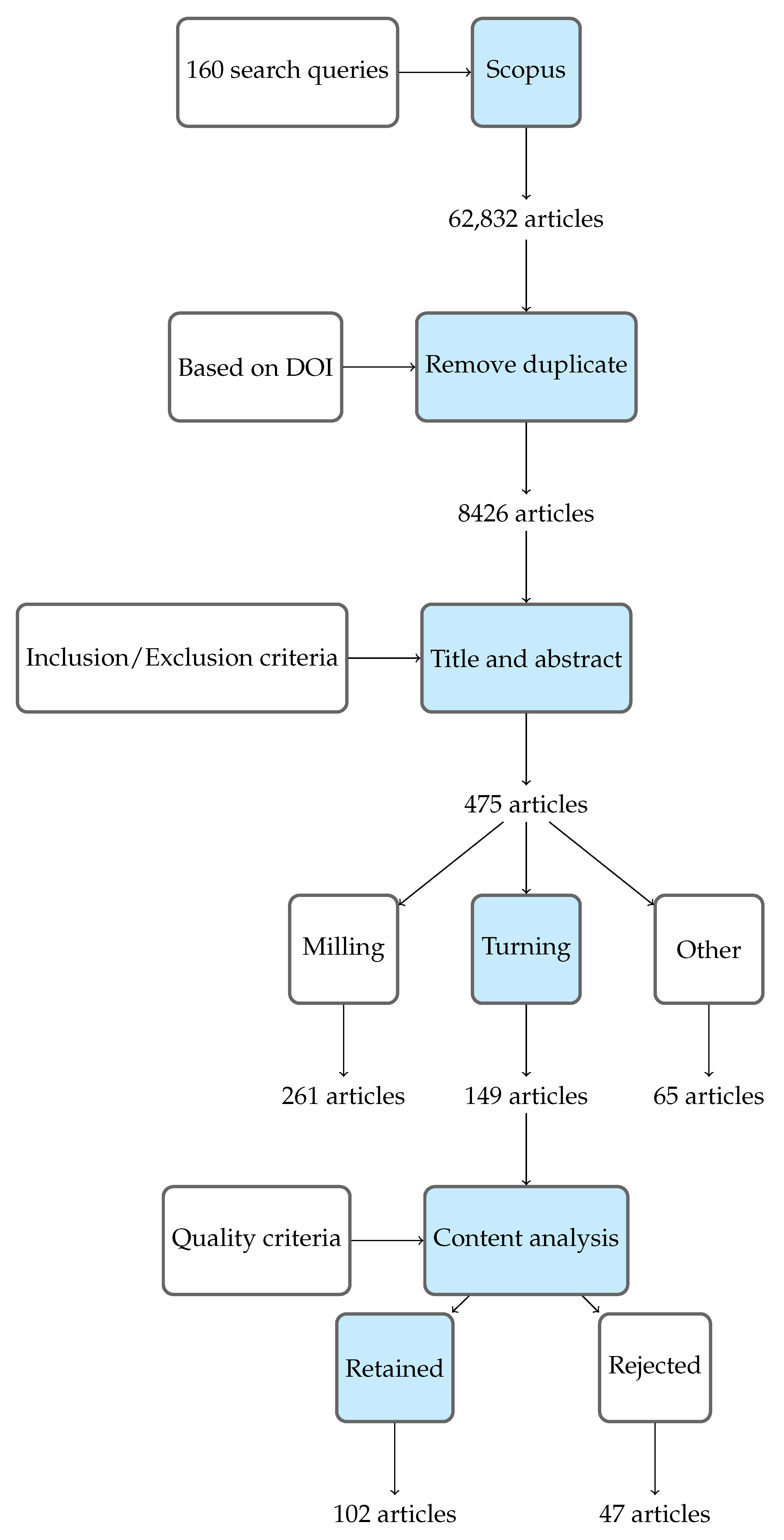
All six stages of this protocol are exposed in the remainder of Section 3. Figure 3 presents a summary of the research protocol with the corresponding results.

3.1. Research Questions

As presented in the introduction, the interest of AI techniques applied in manufacturing is a constantly growing subject. This subject is in fact too broad to be treated in, a single review. In consequence, the main research question of this review is intentionally limited to the use of AI techniques to monitor the tool wear in stable turning operations. The research question is expressed as:

RQ1 

How is the AI used in the framework of monitoring/predicting the condition of tools in a stable turning condition?

The formulation of this research question aims to precisely define the framework of this paper. The concepts of AI and ML have been described in Section 2.2. The words “monitoring/predicting” are used to encompass all monitoring cases, i.e., in real time or with a prediction of the future state of the tool. As many indicators can be used to monitor the tool, the word “condition” is used to encompass them all. The formulation “stable turning condition” aims to reject all papers that discuss chatter or tool breakage detection. As this research question mainly focuses on AI methods applied to the health of the tool, quality-oriented approaches which focus on workpieces are not considered in this review.

The research question is voluntarily broad, such that some sub-questions can be addressed:

RQ2 

What are the most used AI techniques used in this context?

RQ3 

What is the forecasting horizon of each of the identified AI techniques in this context?

RQ4 

What are the most common inputs used with the different identified AI techniques in this context?

RQ5 

What are the most used feature extraction techniques used in this context?

These research questions are answered throughout the SLR analysis process, and they are explicitly answered in Section 7.

3.2. Search Process

3.2.1. Database

To answer the research question, adequate databases should be consulted. The database must be as large as possible and related to the subject to have a representative panel of articles constituting the current state of the art. In this review, it was chosen to use the Scopus database as it regroups a large number of relevant journals from various publishers [28]. Due to the evolution of AI techniques and computing power, it was considered that articles dating from before 2000 were not representative of the current state of the art in the frame of this SLR. Thus, it was chosen to limit the search process over a 20-year period from January 2000 to December 2020. Furthermore, other studies also stated that before 2000 the vast majority of AI techniques used was ANN [29]. A literature review made in 2002 [10] already addresses this part of the literature [10].

3.2.2. Keywords

The search terms must be chosen to be the most general in the framework of the research question. It ensures that the research addresses the topic without introducing bias. The keywords used to perform the search in the Scopus database are listed in

Table 1. List of keywords. Wildcard character (*) includes these different forms of the “tool” word: “tool”, “tools”, and “tooling”.

Tool Part	Aims	Method	Indicator
Cutting tool *	Prediction	Artificial intelligence	Wear
Machining	Monitoring	Machine learning	Remaining useful life
	Reliability	Intelligent data analysis	Condition
	Prognosis	4.0	Data
	Assessment

. A semantic approach was chosen such that each search query is constructed with one element of each semantic part. It was chosen to compose the search query with four parts:

• the tool part;
• the aims part;
• the method part;
• the indicator part.

For the “tool part” in Table 1, the word cutting tool uses the wildcard character (*), which is used to include these different forms of the “tool” word: “tool”, “tools”, and “tooling”. A total of 160 research queries is constructed with this method, creating all possible combinations with the desired composition. The keywords used to build the search query are voluntarily broad and include all machining processes. The main advantage of this approach is that it allows for going through all the possible combinations, but it creates a significant amount of “duplicate” results which must be removed. This last step can easily be realized automatically.

As mentioned previously, the research was done in the Scopus database, each combination of keywords is entered individually, and the results are obtained with the “search within all fields” option. For the results of each piece of research, Scopus provided the following informations: Title, authors, year, DOI, abstract, document type, publisher, number of citation, …

From the 160 search queries, 62,832 articles were obtained. The duplicates were removed based on their DOI. This lead to 8426 unique articles. On average, every search made with this approach yielded 393 results. The most successful search query yielded 3180 results and was

• “machining” AND “prediction” AND “artificial intelligence” AND “data”

With only two results, the least successful search was

• “cutting tool*” AND “prognosis” AND “intelligent data analysis” AND “data”

From the 160 combinations of keywords, 19 combinations gave more than 1000 results. From these 19 combinations, it is possible to generalize a search query that would yield most results into this form:

• “machining” AND (“prediction” OR “monitoring”) AND (“artificial intelligence” OR “machine learning”) AND (“condition” OR “data” OR “wear”)

3.3. Inclusion and Exclusion Criteria

From the previous step in the procedure, 8426 articles are identified. Not all these articles are relevant to answer the research question. To assess the eligibility of each article, it has to be compared with some inclusion and exclusion criteria. These criteria are chosen in accordance with the perspectives of this review and try to be inclusive enough to find all the articles of interest while clearly delineating the research question. These criteria are listed below.

Inclusion Criteria:

IC1 

The paper describes the application of an AI method applied to cutting tools.

IC2 

The paper is about turning operation. This information must be clearly stated in the title or the abstract.

IC3 

The paper is written in English.

IC4 

The AI must provide information on the tool condition.

IC5 

The paper has been published between January 2000 and December 2020.

Exclusion Criteria:

EC1 

The paper must not include instabilities/chatter in the machining process.

EC2 

The paper must not be a review.

Based on titles and abstract of the identified articles, the inclusion and exclusion criteria were applied to obtain 475 results. At this stage, the inclusion criteria IC2 was not applied to obtain an overview of the application of AI techniques in different machining processes. From the 475 results, 149 articles are in turning, 261 are in milling, and 65 in other machining processes (Figure 3). These relevant articles are spread across all search queries; in other words, they are distributed uniformly over the 8426 articles identified. It confirms that the semantic approach used to build the search terms was successful. In the following steps, the criteria IC2 is applied such that only articles about turning are analysed.

Due to the large number of articles and the risk to introduce some bias in the sorting previously described, this stage was performed in parallel simultaneously by two researchers. After the independent rating phase, in case of disagreement, a discussion took place to make a final decision for these articles as proposed by Kitchenham [15]. As it is a manual sorting step, it can introduce some bias into the choice of the selected article depending on the appreciation of the researchers. To measure the inter-rater reliability, the Cohen’s kappa statistic ($\kappa$) was used [30]. This indicator measures the agreement among raters and is computed as:

$$\kappa =\frac{P_o-P_e}{1-P_e}$$

(1)

with $P_o$ (observed value: 0.93) the observed agreement and $P_e$ (observed value: 0.64) the probability of random agreement. After sorting, the obtained $\kappa$ value was 0.8, which indicates that the raters were in “almost perfect agreement” [30]. This means that the defined criteria were applied in the same way by both researchers. This ensures that the vast majority of relevant articles dealing with the subject of this SLR have been identified and provides quality assessment of the sorting process.

3.4. Article Quality Assessment

The previous steps identify 149 articles about turning (Figure 3). These articles were selected based on their title and abstract, but their contents may still not correspond to the research question of this SLR. The quality of the content of the 149 articles is compared with quality criteria that helps to answer the research questions. The quality assessment is often used to assess differences in the execution of studies [15]. In this SLR, this list of quality indicator is proposed:

QA1 

The paper correspond to the inclusion criteria.

QA2 

The paper presents a clear data input description.

QA3 

The origin of the data are clearly defined.

QA4 

The paper clearly describes its methodology.

QA5 

The pre-processing on the data are explicitly mentioned (if any).

QA6 

The paper presents an indicator for the quality of their results.

If two or more of these criteria are not met, the paper is rejected. Based on the quality indicators, the rejected articles are articles that do not contribute to answering the research question or do not provide enough information to be fairly compared with others. The analysis of content and the application of these criteria results in 102 articles retained and 47 articles rejected (Figure 3).

3.5. Data Collection and Data Analysis

By following the procedure previously described, 102 articles are selected to be presented in the SLR (Figure 3). In what follows, two types of analyses are performed:

• A descriptive analysis (Section 4). This part discusses the trends in the literature and shows the state of the art on the research question. Bibliometric information such as year of publication, authors, number of citations are discussed. A text mapping is also presented.
• An in-depth analysis of the AI techniques used (Section 5). A detailed analysis of the content of the articles is carried out and presented in the form of tables. Each category of AI is discussed individually and relevant information in each category are presented. Criteria such as input data, pre-processing, and output are discussed.

4. Bibliometrics Analysis

From the 102 articles identified with the procedure described above (Section 3), a bibliometric analysis is performed. The aim of this analysis is to present the trend in the literature and give a meaningful picture of the state of the art. As described above, this analysis focuses on the 102 previously identified articles from the last 20 years in the context of AI applied to cutting tools in turning operation.

4.1. Distribution in Time

The distribution of the number of publications per year allows for finding if a subject is of interest among researchers. This makes it possible to show trends over the years and reflects the research interest in a subject. Knowledge of these trends allows researchers to align their efforts in particular topics to solve current technological challenges.

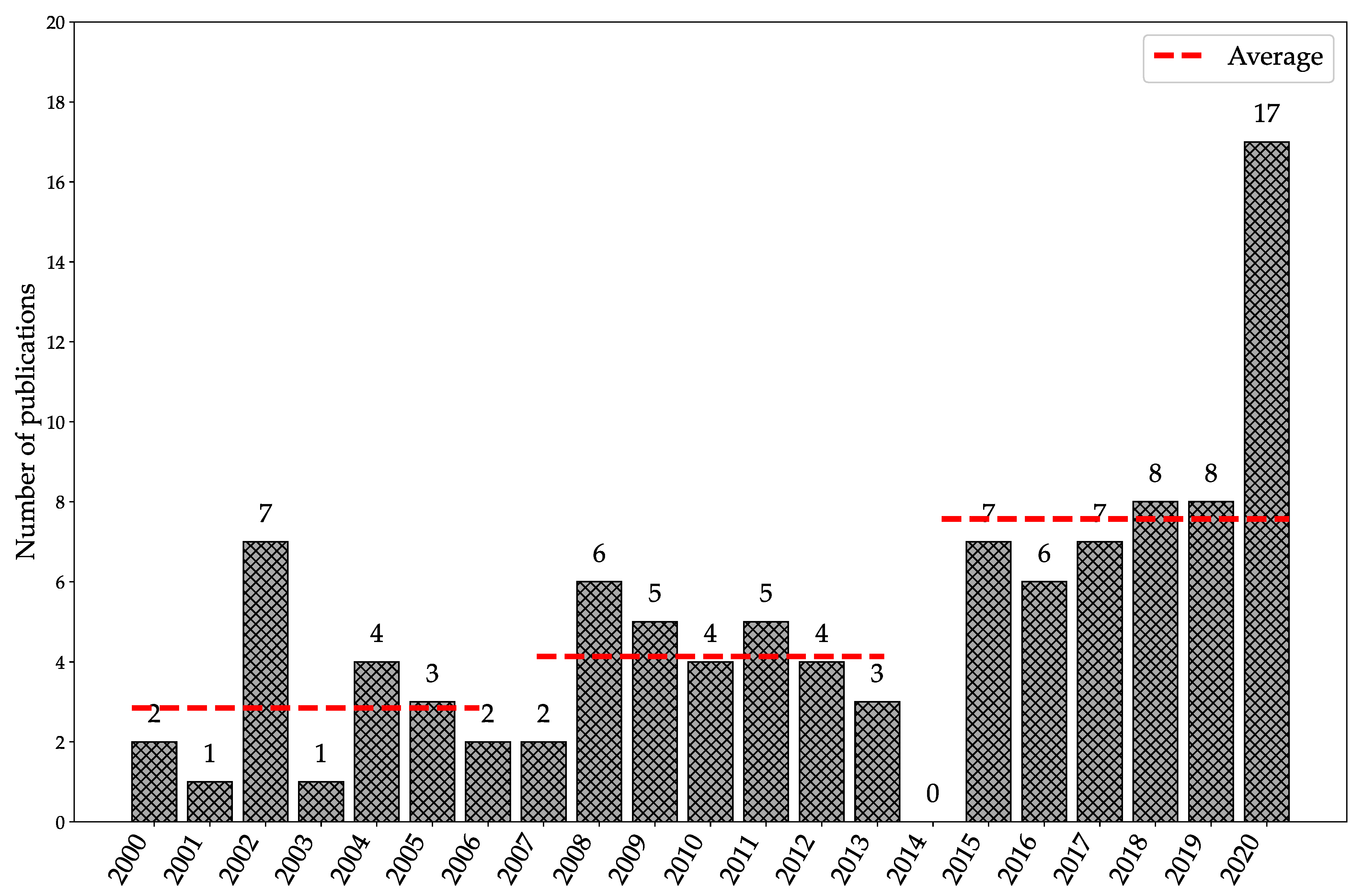
The distribution of publications between 2000 and 2020 is presented in Figure 4. It can be observed that there is a steady growth in the number of articles which reflects the growing interest in the use of AI in the industrial sector. This may be related with the evolution of AI techniques and also the amount of data generated by machine tools in the framework of industry 4.0. From Figure 4, it is possible to divide the timeline into three identical periods of seven years: from the period of 2000 to 2006, there is an average of 2.85 articles per year, from the period of 2007 to 2013, there is an average of 4.14 articles per year and from the period of 2013 to 2020, there is an average of 7.57 articles per year. It is observed that the year 2020 was particularly rich in the number of publications which may indicate the rise of a hot topic in the literature.

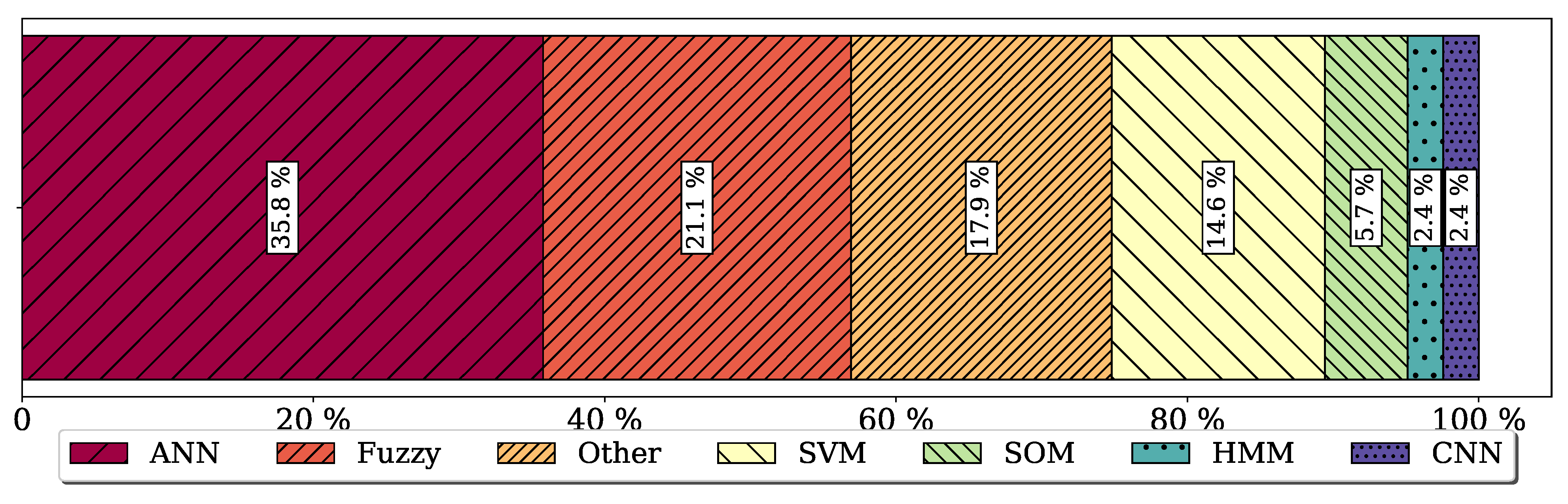
4.2. Repartition of AI Type

From the content analysis of the selected papers, seven “types” of AI stand out. The categorization is the reflection of the occurrence of these techniques in the literature:

• Artificial Neural Network (ANN) (Appendix B.1).
• Fuzzy approach (FIS and ANFIS models) (Appendix B.2).
• Support Vector Machine (SVM) (Appendix B.3).
• Self Organizing Map (SOM) (Appendix B.4).
• Hidden Markov Model (HMM) (Appendix B.5).
• Convolutional Neural Network (CNN) (Appendix B.6).
• Other. This category regroups techniques that individually are not sufficiently represented to have their own category. It includes AI techniques such as: decisions trees, K-nearest neighbour classifier, etc.

These different techniques are the subject of an in-depth analysis in Section 5, including tables summarizing the review results. To be exhaustive and take into account articles that in addition to the AI approach addressed a non-AI approach, the category “other (not AI)” has been added.

The repartition of the type of AI used to monitor the tool wear is presented in Figure 5. From this figure, it is observed that the majority of articles focuses on the following AI techniques: ANN, Fuzzy and SVM. These three techniques represent about 60% of all articles. The other techniques, i.e., SOM, HMM, CNN and “other” together represent the remaining 40% of the literature.

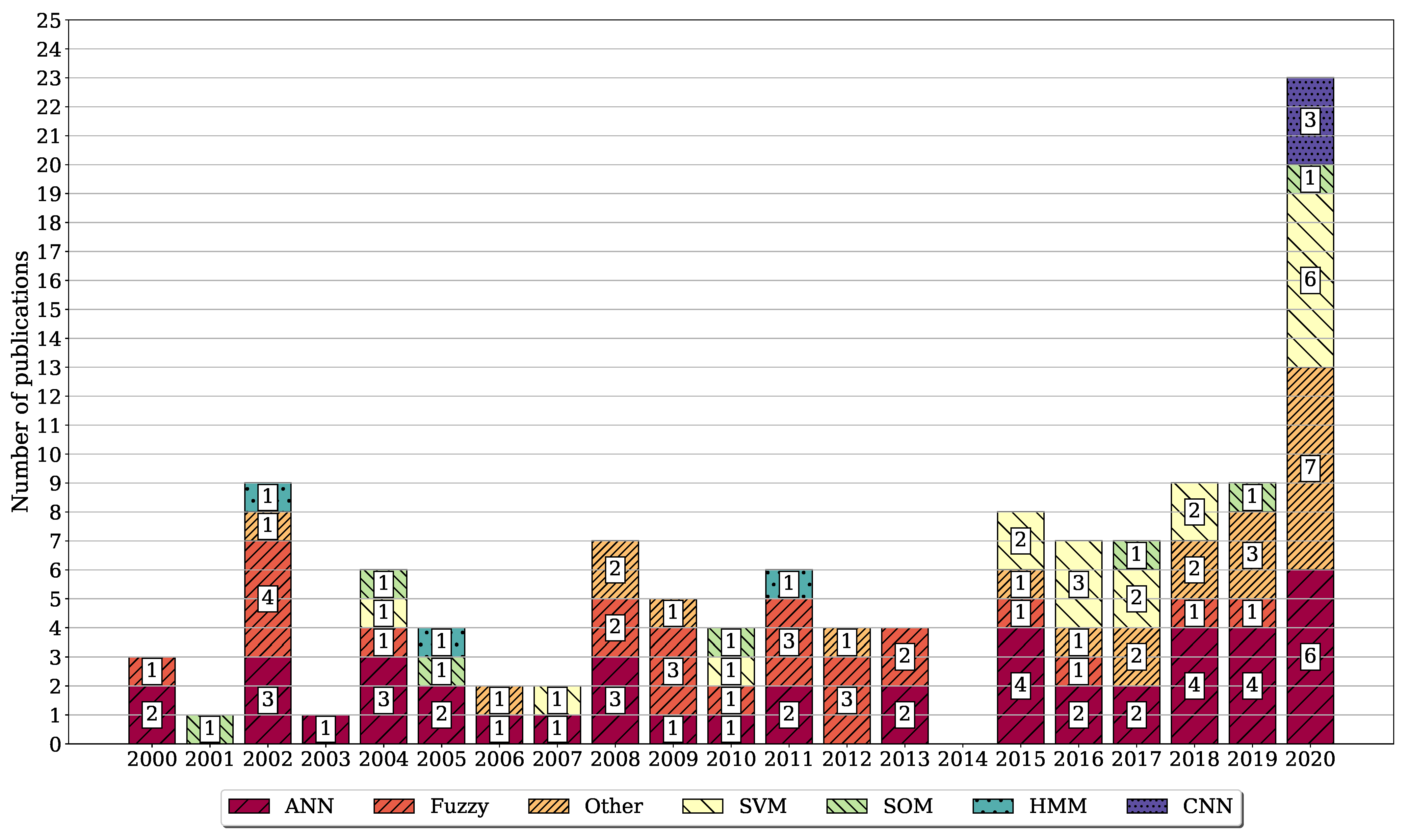
The repartition of the type of AI by year is presented in Figure 6. It should be noted that some articles discuss several independent AI techniques, which explains why the numbers are not consistent with the repartition by year in Figure 4. This figure allows observing some trends in the literature:

• The interest for the ANN approach occupies an almost constant proportion of the literature through the years.
• The SVM approach has seen a growing interest in the last five years.
• The fuzzy logic approach aroused great interest up to 2011, but it seems less represented in recent years.
• Techniques such as HMM and SOM are not sufficiently represented to observe any tendencies.
• The CNN approach was first observed in 2020. Therefore, no conclusion can be drawn as to its use. It will be necessary to monitor its use in future years to observe if this is a hot topic of ongoing research.
• The other AI techniques have a growing interest too. This may indicate an interest to test new approaches.

The choice to carry out an analysis of the literature over the last 20 years therefore makes it possible to observe the evolution in interest of each of the AI techniques. This allows for identifying all the approaches that have been tried and which approaches are raising the most interest for future trends.

4.3. Citations Analysis

Analysing the number of citations helps to identify the most influential papers in a subject. In this SLR, seven types of AI have been identified, and the top 3 of the most cited articles in each technique is presented in Table 2. The number of citations comes from the Scopus database and reports this value as of 1 January 2021. In Table 2, as the HMM and CNN approaches include only three articles, all articles are listed, resulting in a citation number of 0 for 3 articles.

Hereafter, the top 3 of the most cited articles in all categories of AI are presented (in boldfacetype in Table 2):

• The most cited article is [31] (Salgado and Alonso, 2007) and concerns the uses of SVM with easily accessible signals such as sound, motor current and cutting parameters to make a real-time estimation of ${\mathrm{VB}}_B$.
• The second paper that receives the most attention is [32] (Wang et al., 2002). It uses an HMM approach using a pre-processed vibration signal to classify the state of the tool (“new tool” or “worn tool”).
• The third most cited paper is [33] (Balazinski et al., 2002) and concerns the use of ANN and Artificial Neural Network Based Fuzzy Inference System (ANNBFIS) with the feed rate, cutting force and feed force as input signals to estimate the tool wear (${\mathrm{VB}}_B$).

On average, all identified articles are cited 18 times. Even if the HMM approach is not strongly represented in the literature (Section 4.1), it appears that that publication [32] has been cited a significant number of times. However, this citation analysis may present some bias. Indeed, for a paper to accumulate citations, it has to be published for a sufficient time to be read and cited. It is therefore normal to observe a majority of papers published before 2015 in this analysis. Note that the number of citations was not always available for all 102 articles.

Table 2. Top 3 most cited articles by AI techniques, three globally most cited articles in boldface type.

Technique	No. Citation	Article
ANN	94	[33] “Tool condition monitoring using artificial intelligence methods” Balazinski et al., 2002
	90	[34] “Online metal cutting tool condition monitoring” Dimla and Lister 2000
	83	[35] “Prediction of flank wear by using back propagation neural network modelling when cutting hardened H-13 steel with chamfered and honed CBN tools” Özel and Nadgir 2002
Fuzzy	94	[33] “Tool condition monitoring using artificial intelligence methods” Balazinski et al., 2002
	63	[36] “Tool wear monitoring using neuro-fuzzy techniques: a comparative study in a turning process” Gajate et al., 2012
	61	[37] “Online tool wear prediction system in the turning process using an adaptive neuro-fuzzy inference system” Rizal et al., 2013
SVM	135	[31] “ An approach based on current and sound signals for in-process tool wear monitoring” Salgado and Alonso 2007
	45	[38] “On machine tool prediction of flank wear from machined surface images using texture analyses and support vector regression” Dutta et al., 2016
	33	[39] “Identification of features set for effective tool condition monitoring by acoustic emission sensing” Sun et al., 2004
SOM	94	[40] “Wear monitoring in turning operation using vibration and strain measurements” Scheffer and Heyns 2001
	17	[41] “ Tool wear monitoring—an intelligent approach” Rao and Srikant 2004
	10	[42] “Condition monitoring of the cutting process using a self organized spiking neural network map” Silva 2010
Other	69	[43] “ Tool condition monitoring based on numerous signal features” Jemielniak et al., 2012
	15	[44] “Fusion of hard and soft computing techniques in indirect online tool wear monitoring” Sick 2002
	12	[45] “Metacognitive learning approach for online tool condition monitoring” Pratama et al., 2019
HMM	125	[32] “ Hidden Markov Model-based tool wear monitoring in turning” Wang et al., 2002
	20	[46] “ A comparative evaluation of neural networks and hidden Markov models for monitoring turning tool wear” Scheffer et al., 2005
	0	[47] “Tool wear intelligence measure in cutting process based on HMM” Kang and Guan 2011
CNN	1	[9] “ A qualitative tool condition monitoring framework using convolution neural network and transfer learning” Mamledesai et al., 2020
	0	[48] “Indirect cutting tool wear classification using deep learning and chip colour analysis” Pagani et al., 2020
	0	[49] “A U-net-based approach for tool wear area detection and identification” Miao et al., 2021

Table 2. Top 3 most cited articles by AI techniques, three globally most cited articles in boldface type.

Technique	No. Citation	Article
ANN	94	[33] “Tool condition monitoring using artificial intelligence methods” Balazinski et al., 2002
	90	[34] “Online metal cutting tool condition monitoring” Dimla and Lister 2000
	83	[35] “Prediction of flank wear by using back propagation neural network modelling when cutting hardened H-13 steel with chamfered and honed CBN tools” Özel and Nadgir 2002
Fuzzy	94	[33] “Tool condition monitoring using artificial intelligence methods” Balazinski et al., 2002
	63	[36] “Tool wear monitoring using neuro-fuzzy techniques: a comparative study in a turning process” Gajate et al., 2012
	61	[37] “Online tool wear prediction system in the turning process using an adaptive neuro-fuzzy inference system” Rizal et al., 2013
SVM	135	[31] “ An approach based on current and sound signals for in-process tool wear monitoring” Salgado and Alonso 2007
	45	[38] “On machine tool prediction of flank wear from machined surface images using texture analyses and support vector regression” Dutta et al., 2016
	33	[39] “Identification of features set for effective tool condition monitoring by acoustic emission sensing” Sun et al., 2004
SOM	94	[40] “Wear monitoring in turning operation using vibration and strain measurements” Scheffer and Heyns 2001
	17	[41] “ Tool wear monitoring—an intelligent approach” Rao and Srikant 2004
	10	[42] “Condition monitoring of the cutting process using a self organized spiking neural network map” Silva 2010
Other	69	[43] “ Tool condition monitoring based on numerous signal features” Jemielniak et al., 2012
	15	[44] “Fusion of hard and soft computing techniques in indirect online tool wear monitoring” Sick 2002
	12	[45] “Metacognitive learning approach for online tool condition monitoring” Pratama et al., 2019
HMM	125	[32] “ Hidden Markov Model-based tool wear monitoring in turning” Wang et al., 2002
	20	[46] “ A comparative evaluation of neural networks and hidden Markov models for monitoring turning tool wear” Scheffer et al., 2005
	0	[47] “Tool wear intelligence measure in cutting process based on HMM” Kang and Guan 2011
CNN	1	[9] “ A qualitative tool condition monitoring framework using convolution neural network and transfer learning” Mamledesai et al., 2020
	0	[48] “Indirect cutting tool wear classification using deep learning and chip colour analysis” Pagani et al., 2020
	0	[49] “A U-net-based approach for tool wear area detection and identification” Miao et al., 2021

4.4. Journal Analysis

The 102 identified articles appear in 61 journals from 23 publishers. The most influential journals with more than three articles cited in this SLR are identified:

• The International Journal of Advanced Manufacturing Technology is the most represented journal with 10 articles;
• Journal of Intelligent Manufacturing is the second most represented journal with eight articles;
• Proceedings of the Institution of Mechanical Engineers, Part B: Journal of Engineering Manufacture with five articles;
• International Journal of Machine Tools and Manufacture with four articles.

The other articles come from either journals or conference proceedings that generally have only a single article taken into account in the framework of this SLR.

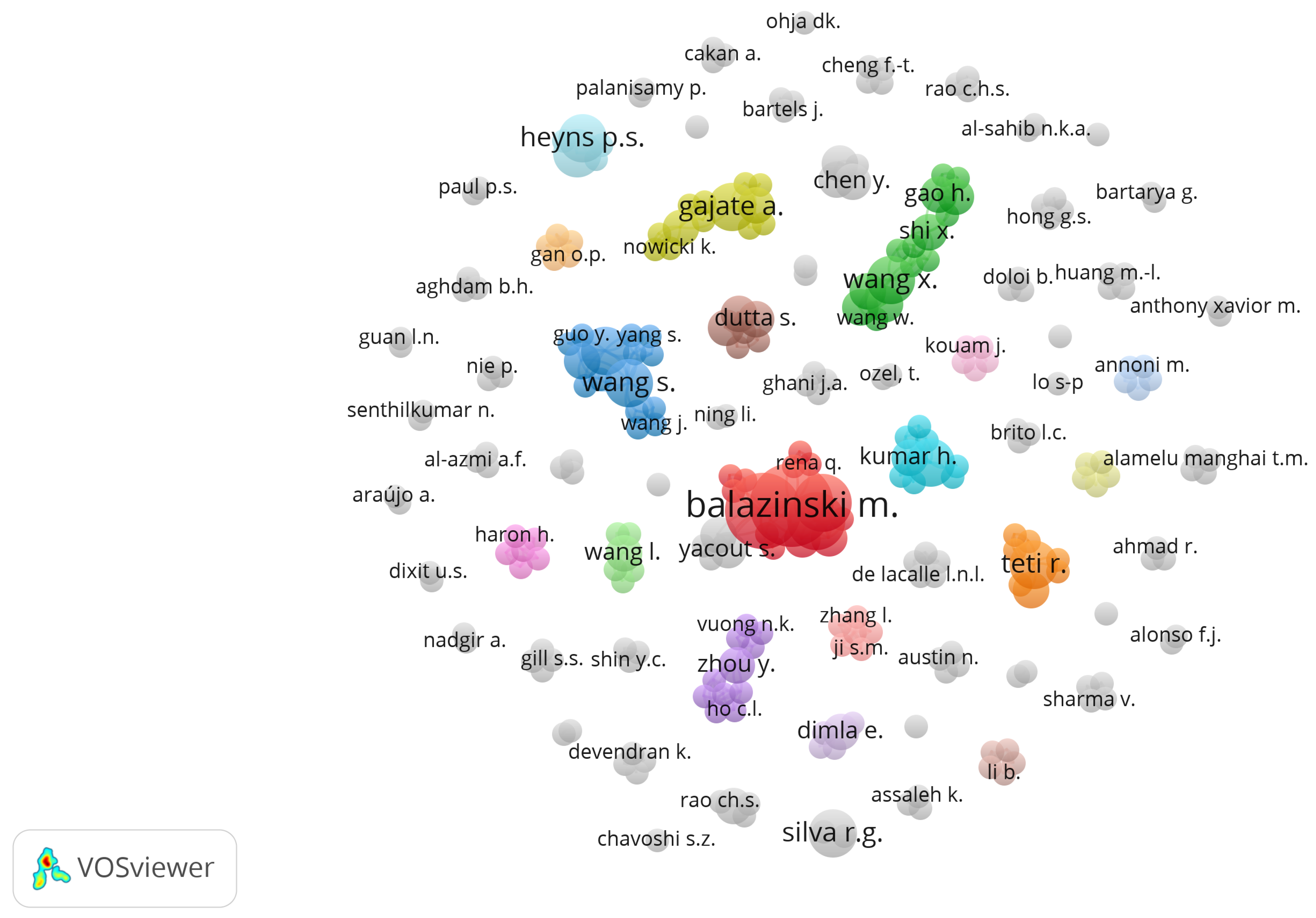
4.5. Authors

The identified articles were written by 280 different authors. Among those, only 13 authors have published more than three articles on this subject.

A co-authorship analysis is performed using VOSViewer (a tool for creating, visualizing and exploring meaningful map of items of interest [50]). A mapping of the different authors is presented in Figure 7. The size of each item (authors name and associated circles) indicates the occurrence of the authors in the literature. A larger circle means that the corresponding author appeared more in this SLR. Each cluster represents an author group, i.e., usual co-authors. The larger a cluster, the more authors there are in it. It is observed that there are some clusters which are larger and bigger than the others. This is generally a specific lab that works on the subject of this SLR. It is observed that most of the clusters are isolated, and there is no link between them. This does not mean that the authors do not cite each other, but it does indicate that there is very little inter-lab collaboration in the redaction of articles beyond usual co-authors.

5. In Depth Analysis

Below, an analysis of the content of the articles is carried out from the different categories of AI, namely ANN, Fuzzy, SVM, SOM, HMM, CNN, and other. This analysis is broken down into two stages:

• The content of the articles is presented in table form (

  Table A1. General summary of ANN-related publications.

  Article	Method	Material	Input	Output	Pre-Processing	Comments
  [53]	ANN	Inconel 718	Cutting forces AE Vibration	Estimation of VB	Time/frequency	3 layers: 3 to 7 neurons in the hidden layer
  [71]	Recurrent neural network (RNN)	mild steel	Cutting forces Vibration Acoustic (audible)	Estimation of VB	Statistic	Best performance with 6 to 9 neurons in hidden layers
  [54]	ANN	steel EN8	Cutting speed Cutting forces Feed Depth of cut	Estimation of VB	None	3 layers: 5 inputs; 1hidden (5 to 10 neurons); 1 output
  [55]	ANN	hardened bearing steel (61HRC)	Cutting forces Vibration	Estimation of VB	Statistic	Multi layer perceptron
  [111]	Regression neural networks	high manganese cast steel	Cutting speed Cutting forces Vibration Feed Depth of cut Temperature	Estimation of VB	Normalization
  [70]	Generalized regression neural network with improved fruit fly optimzation	high manganese cast steel	Cutting speed Feed Depth of cut	Estimation of VB	Normalization	93% accuracy
  [52]	Back Propagation NN	aluminum alloy 7050	Vibration Acoustic (audible)	Classification	Time/frequency	3 layers: 8-11-3; 3 states classification up to 92.5% accuracy
  [72]	ANN	steel	Other	RUL	None
  [56]	ANN	Ti6Al4V	AE Vibration	Estimation of VB	Statistic	Best results with 3-3-1 and 3-6-1
  [76]	ANN, fuzzy logic and regression (not AI)	AISI 4140	Cutting speed Feed Depth of cut	Estimation of VB	None
  [66]	ANN	AISI 4140	Cutting speed Cutting forces Vibration Feed Depth of cut	Estimation of VB	None	shape: 5-14-6-1-1
  [57]	ANN	AISI 316	Cutting forces AE Vibration	Other	Time/frequency Statistic	3 layers: 6-x-1. Output: percentage of tool life
  [74]	ANN and case based reasoning	steel AISI 304; AISI D2; AISI 52100	Cutting speed Feed Depth of cut Other	RUL Other		Output: Tool life and tool-shim interface temperature
  [112]	ANN	steel (AISI 4340)	Cutting speed Feed Depth of cut
  [75]	ANN and regression model (not AI)	3 different steel	Cutting speed Feed Depth of cut Other	Estimation of VB Other	None	Comparison with multiple linear regression model. Output: surface roughness and flank wear
  [68]	ANN and SVM	steel (AISI 4340 AND 52100 hardenend)	Surface texture	Estimation of VB	None	Reflectiveness of the surface; 28 ANN: 6 Multi Layer Perceptron (MLP), 3 MLP with Principal Component Analysis (MLPPCA), 3 Generalized FeedForward (GFF), 3 Radial Basis Function, 3 Time Delay Neural Network, 3 time-lag recurrent network (TLRN), 3 Recurrent Network, 2 linear regression (LR), 1 probabilistic neural network (PNN) and 1 SVM models
  [67]	ANN and regression (not AI)	steel (AISI 4340)	Cutting speed Cutting forces Feed Depth of cut Other Temperature	Estimation of VB	Other	Architecture: 6-4-5-4-1. Comparison with regression
  [58]	ANN and CANFIS	7075 alloy	Cutting speed Feed Depth of cut	Estimation of VB	None	Co-Active Neuro Fuzzy Inference System (CANFIS)
  [113]	ANN	grey cast iron	Cutting speed Cutting time Feed Depth of cut	Other	None	Output: Cutting forces (estimation of flank wear)
  [114]	ANN and polynomial classifiers	mild steel	Cutting speed Cutting forces AE Cutting time Feed	Estimation of VB	Other Statistic	ANN 90% accuracy and classifier 85%
  [115]	ANN	AISI 52100 bearing steel	Cutting speed Cutting time Feed Depth of cut Other	Estimation of VB	Normalization	3 layers: 5-7-1
  [59]	ANN and regression model (not AI)	steel AISI H13	Cutting speed Feed Depth of cut	Estimation of VB Other	None	3 layers and 5 neurons in the hidden layer. Output: Flank wear and surface roughness
  [60]	ANN	EN-8 steel	Cutting speed Cutting time Feed Depth of cut Other Temperature		None	3 layers and 5 neurons in the hidden layers. There is a mathematical relationship to predict the tool wear. The AI does not predict directly the wear
  [35]	ANN	hardened (55HRC) H-13 steel tube	Cutting speed Cutting forces Cutting time Other	Estimation of VB	Other
  [77]	Neural networks	Experiment AISI 1045 steels	Cutting speed Feed Depth of cut Motor info	Estimation of VB	Other	Machine learning process optimal linear associative memory (MLP OLAM)
  [116]	Random Forest; gradient boosting regression, neural network and Support vector regression	hardened steel (58 HRC)	Cutting speed Cutting forces AE Vibration Feed Depth of cut Other	Estimation of VB	Time/frequency Statistic Frequency domain
  [104]	Classifier: Decision tree, K-neighbour, Random forest; Regressor: MLP, Random Forest, SVM, Naive Bayes, gradient boosting	Generation on Python (turning case)	Cutting forces Motor info	Classification Estimation of VB	None	2 states classification
  [61]	ANN and Response Surface Methodology (RSM) (Not AI)	/	Cutting speed Feed Depth of cut	Estimation of VB	None	3 layers: 5 neurons in the hidden layer; Activation function: “tansig”; Better results with the AI approach
  [117]	MLP ANN	Die steel	Vibration	Classification	Frequency domain	2 states classification; 87% accuracy
  [62]	ANN	Ti6Al4V	Cutting forces AE	Estimation of VB	Statistic	3 layers with 9, 18 or 27 neurons in the hidden layer
  [118]	ANN (MLFFNN)	steel EN 24	AE	Estimation of VB	Frequency domain
  [41]	SOM, neuro-fuzzy, ANN	EN-8 Steel	Cutting forces	Classification Estimation of VB	None	ANN: 3 layers: 2-3-1; SOM: classification
  [63]	ANN	/	Acoustic (audible) Surface texture	Estimation of VB	Other Frequency domain	3 layers: 3-4-1
  [85]	Hybrid: ANN and fuzzy modelling	SAE 6150 chromim-vanadium alloy steel	Cutting forces AE Vibration	Estimation of VB	Statistic Frequency domain
  [34]	ANN	EN24 steel	Cutting forces Vibration	Classification	Normalization	3 layers MLP: 7-20-1; 7 States classification
  [64]	ANN	steel aisi 1040	Cutting forces Cutting time Surface roughness Other Temperature	Estimation of VB	Normalization	3 layers: 3 neurons in the hidden layer
  [119]	ANN	100Cr-6 and 54CrV4	Cutting speed Cutting forces AE Feed	Estimation of VB	Statistic Frequency domain	SOM for correlation analysis
  [46]	ANN and HMM	From another study	Cutting forces	Classification Estimation of VB	Time/frequency Statistic Frequency domain	Comparison between the two approaches: similar results
  [33]	ANN; Fuzzy decisions support logic (rules set by the researcher); Artificial Neural Network Based Fuzzy Inference System (ANNBFIS)	/	Cutting forces Feed	Estimation of VB	None	For ANN 3 layers: 5 neurons in the hidden layers
  [65]	ANN	Another study - EN-24-steel	Cutting speed Feed Depth of cut	Estimation of VB	None	3 layers: 3-7-1. More than 90% accuracy
  [73]	Neural network	mild steel	Cutting speed Feed Depth of cut	RUL	Normalization	Comparison with regression
  [101]	ANFIS and BPNN	Stainless steel 304 L	Cutting forces	Classification Estimation of VB	Statistic	2 states classification
  [120]	ANN	hardened AISI 52100 (literature) and experiment on AISI H-13	Cutting speed Cutting forces Feed Other	Estimation of VB Other	Statistic	3 layers: 8 to 13 neurons in the hidden layer. Comparison with regression: AI perform better
  [121]	ANN	AISI D2	Cutting speed Cutting time Feed	Estimation of VB	None

  ,

  Table A2. General summary of fuzzy logic related publications.

  Article	Method	Material	Input	Output	Pre-Processing	Comment
  [83]	Decision tree (j48) and fuzzy logic	steel	Vibration	Classification	Statistic	95% accuracy
  [76]	ANN, fuzzy logic and regression (not IA)	AISI 4140	Cutting speed Feed Depth of cut	Estimation of VB	None
  [84]	Type 2 fuzzy model	Titanium Metal Matrix Composite	AE	Estimation of VB	Other
  [85]	Hybrid: ANN and fuzzy modelling	SAE 6150 chromim-vanadium alloy steel	Cutting forces AE Vibration	Estimation of VB	Statistic Frequency domain
  [86]	Takagi–Sugeno–Kang (TSK) Fuzzy Approach Based on Subtractive Clustering Method	steel	Cutting forces Feed	Estimation of VB	None
  [87]	Takagi–Sugeno–Kang (TSK) Fuzzy Approach Based on Subtractive Clustering Method	steel	Cutting forces	Estimation of VB	None
  [88]	Fuzzy method	/	Cutting forces Feed	Estimation of VB	None	2 approaches: one with the knwoledge given by the researcher and one automatic genetic algorithm
  [33]	ANN; Fuzzy decisions support logic (rules set by the researcher); Artificial neural network based fuzzy inference system (ANNBFIS)	/	Cutting forces Feed	Estimation of VB	None	For ANN 3 layers: 5 neurons in the hidden layers

  ,

  Table A3. General summary of neuro-fuzzy related publications.

  Article	Method	Material	Input	Output	Pre-Processing	Comment
  [89]	ANFIS	steel 1215.	Cutting forces	Estimation of VB	Time/frequency	5 layers; 4 different activation function: sigmoid, triangular, gaussian, bell-shaped
  [90]	Type 2 basis function network	steel/ inconel/ Ti6Al4V	AE Vibration Motor info	Estimation of VB	Normalization
  [91]	ANFIS	steel	Cutting forces Feed	Estimation of VB	Statistic
  [37]	ANFIS	hardened JIS S45C carbon steel	Cutting speed Feed Depth of cut Other	Estimation of VB	Other	Features extraction with Z-filter
  [36]	ANFIS	From another study	Cutting forces AE Vibration Cutting time	Estimation of VB	Normalization	Inductive, transductive and evolving neuro-fuzzy systems
  [92]	ANFIS	cryogenically treated AISI M2 high speed steel	Cutting speed Cutting time Other	Estimation of VB	None
  [93]	ANFIS	D2 X115Cr VMo121 steel	Surface texture Temperature Motor info	Estimation of VB	None	Accuracy up to 98%
  [94]	Fuzzy with a new Takagi–Sugeno–Kang (TSK) modelling	steel	Cutting forces Feed	Estimation of VB	None
  [58]	ANN and CANFIS	7075 alloy	Cutting speed Feed Depth of cut	Estimation of VB	None	Co-Active Neuro Fuzzy Inference System
  [95]	Transductive-Weighted Neuro-Fuzzy Inference System (TWNFIS)	From another study	Cutting forces AE Vibration	Estimation of VB	None	More than 90% accuracy
  [96]	ANFIS compared with Hybrid approach	steel EN 24 and FG15	Cutting forces AE Vibration Cutting time	Estimation of VB	Normalization	comparison between Transductive Weighted Neuro-Fuzzy Inference System (TWNFIS), ANFIS and Hybrid Incremental Modeling (HIM). HIM outperform the other
  [41]	SOM, neuro-fuzzy, ANN	EN-8 Steel	Cutting forces	Classification Estimation of VB	None	ANN: 3 layers: 2-3-1; SOM: classification
  [97]	Evolving extended Takagi–Sugeno based neuro-fuzzy algorithm	Inconel 718	Cutting forces AE	Estimation of VB	Statistic
  [98]	Localized fuzzy neural network (LFNN)	45 middle carbide steel workpiece	Cutting forces AE	Classification	Time/frequency
  [33]	ANN; Fuzzy decisions support logic (rules set by the researcher); Artificial neural network based fuzzy inference system (ANNBFIS)	/	Cutting forces Feed	Estimation of VB	None	For ANN 3 layers: 5 neurons in the hidden layers
  [99]	ANFIS	steel	Cutting forces AE	Classification	Statistic	Best with triangular and bell function
  [100]	ANFIS	FG15 cast iron	Cutting forces AE Vibration Cutting time	Estimation of VB	Other	Around 82% accuracy
  [101]	ANFIS and Back Propagation NN	Stainless steel 304 L	Cutting forces	Classification Estimation of VB	Statistic	2 states classification

  ,

  Table A4. General summary of SVM-related publications.

  Article	Method	Material	Input	Output	Pre-Processing	Comment
  [51]	SVM	high strength steel (45CrNiMoVA)	Cutting forces Vibration Surface texture	Estimation of VB	Time/frequency Statistic Frequency domain	Grid search-SVR, Genetic algorithm SVR, Particle swarm optimizer-SVR and Grid-search SVR
  [103]	Gravitational search algorithm coupled with least square support vector machine model	steel	Cutting forces	Classification	Time/frequency Normalization Statistic	3 states classification
  [2]	SOM; SVM; k-nearest neighbour	steel AISI D6	Vibration	Classification	Normalization Statistic Frequency domain	Accuracy up to 92%; 2 states classification
  [102]	SVR modified	/	Other	Prediction of Vb	Normalization	Forecasting at $t+1$
  [122]	SVM and decision tree	steel (1.4542)	Motor info	Classification	Time/frequency Normalization Frequency domain	2 states classification; above 90% accuracy
  [123]	SVM	ZMn13 high manganese cast steel	Cutting speed Cutting time Feed Depth of cut	Estimation of VB	None	Nelder–Mead Leave One Out-Least squares Support Vector Machines (NM-LOO-LSSVM), Particle Swarm Optimization-LSSVM (PSO-LSSVM) and LSSVM. Best performances with NM-LOO-LSSVM
  [124]	SVM	superalloy	AE Acoustic (audible) Feed Depth of cut Motor info	Classification Estimation of VB	Time/frequency Other	Optimization with genetic alogrithms
  [68]	ANN and SVM	steel (AISI 4340 AND 52100 hardened)	Surface texture	Estimation of VB	None	Reflectiveness of the surface; 28 ANN: 6 Multi Layer Perceptron (MLP), 3 MLP with Principal Component Analysis (MLPPCA), 3 Generalized FeedForward (GFF), 3 Radial Basis Function, 3 Time Delay Neural Network, 3 time-lag recurrent network (TLRN), 3 Recurrent Network, 2 linear regression (LR), 1 probabilistic neural network (PNN) and 1 SVM models
  [116]	Random Forest; gradient boosting regression, neural network and Support vector regression	hardened steel (58 HRC)	Cutting speed Cutting forces AE Vibration Feed Depth of cut Other	Estimation of VB	Time/frequency Statistic Frequency domain
  [104]	Classifier: Decision tree, K-neighbour, Random forest; Regressor: MLP, Random Forest, SVM, Naive Bayes, gradient boosting	Generation on Python (turning case)	Cutting forces Motor info	Classification Estimation of VB	None	2 states classification
  [105]	v-SVR	steel #50	Cutting forces	Estimation of VB	Time/frequency Statistic	Comparison with BPNN
  [125]	SVM	C50 steel	Surface texture	Classification	Other	3 states classification
  [38]	SVM	C50 steel	Surface texture	Estimation of VB	Other
  [126]	SVM	GH4169	AE	Classification	Time/frequency Other Frequency domain	4 states classification
  [31]	LSSVM	steel AISI 1040	Cutting forces Acoustic (audible)	Estimation of VB	Statistic
  [39]	SVM	ASSAB705/760 steel	AE	Classification	Time/frequency Statistic	80-85% accuracy
  [106]	v-SVR	#50 steel	Cutting forces	Classification	Normalization Statistic	2 states classification. 96% accuracy
  [127]	SVM	AISI 01	Surface texture	Estimation of VB	Other	Genetic algorithm

  ,

  Table A5. General summary of SOM-related publications.

  Article	Method	Material	Input	Output	Pre-Processing	Comment
  [2]	SOM; SVM; k-nearest neighbour	steel AISI D6	Vibration	Classification	Normalization Statistic Frequency domain	Accuracy up to 92%; 2 states classification
  [107]	SOM	steel EN1A1	Cutting forces Vibration Acoustic (audible) Feed Motor info	Classification	Statistic Frequency domain
  [128]	SOM	mild steel	AE Vibration Cutting time	Classification	Statistic
  [42]	Self organizing spiking neural network map	mild steel	Cutting forces Vibration Acoustic (audible)	Classification	Statistic Frequency domain
  [41]	SOM, neuro-fuzzy, ANN	EN-8 Steel	Cutting forces	Classification Estimation of VB	None	ANN: 3 layers: 2-3-1; SOM: classification
  [40]	SOM	Industrial in South Africa (piston manufacturer)	Cutting forces Vibration	Classification	Time/frequency Statistic Frequency domain	3 × 3 output
  [129]	Self organizing map (SOM)	cast iron	Cutting forces Vibration	Classification	Time/frequency Statistic Frequency domain

  ,

  Table A6. General summary of HMM-related publications.

  Article	Method	Material	Input	Output	Pre-Processing	Comment
  [47]	HMM	45# steel	Cutting forces Vibration	Classification	Other Normalization Frequency domain
  [46]	ANN and HMM	From another study	Cutting forces	Classification Estimation of VB	Time/frequency Statistic Frequency domain	Comparison between the 2 approaches: similar results
  [32]	Discrete Hidden Markov Model (DHMM)	AISI 8620 steel	Vibration	Classification	Time/frequency	2 states classification; more than 97% accuracy

  ,

  Table A7. General summary of CNN-related publications.

  Article	Method	Material	Input	Output	Pre-Processing	Comment
  [49]	convolutional neural network (U-Net)	45# steel	Surface texture	Estimation of VB	Other
  [48]	CNN and functional data analysis	low carbon steel (25CrMo4)	Surface texture	Classification	Other	3 states classification; around 90% accuracy;
  [9]	CNN	steel	Surface texture	Classification	Other	2 states classification

  and

  Table A8. General summary of publications related to various other methods.

  Article	Method	Material	Input	Output	Pre-Processing	Comment
  [130]	Logical Analysis of data (AI classifier); Logical analysis of survival curves (LASC)	titanium metal matrix composite	Cutting forces	Remaining Useful Life (RUL)	None	Non AI outperform AI
  [2]	SOM; SVM; k-nearest neighbour	steel AISI D6	Vibration	Classification	Normalization Statistic Frequency domain	Accuracy up to 92%; 2 states classification
  [131]	Nearest-Neighbour-like algorithm using non-nested Generalized Exemplar (NNGE)	steel	Vibration	Classification	Statistic	4 states classification up to 100% accuracy
  [83]	Decision tree (j48) and fuzzy logic	steel	Vibration	Classification	Statistic	95% accuracy
  [122]	SVM and decision tree	steel (1.4542)	Motor info	Classification	Time/frequency Normalization Frequency domain	2 states classification; above 90% accuracy
  [132]	linear regression, decision trees, random forests, k-nearest neighbours, adaptive boosting, bootstrap aggregating and gradient boosting	inconel 718	Cutting forces	Estimation of VB	Statistic
  [133]	Hybrid dynamic neural network (HDNN)	steel (different alloy)	Motor info	Estimation of VB	Statistic
  [134]	Logical analysis of data (LAD)	steel (AISI 1045)	Cutting forces Feed	Classification	None
  [74]	ANN and case based reasoning	steel AISI 304; AISI D2; AISI 52100	Cutting speed Feed Depth of cut Other	RUL Other		Output: Tool life and tool-shim interface temperature
  [135]	Novelty detection	steel	Cutting forces	Estimation of VB	Statistic Frequency domain	Up to 100% accuracy
  [114]	ANN and polynomial classifiers	mild steel	Cutting speed Cutting forces AE Cutting time Feed	Estimation of VB	Other Statistic	ANN 90% accuracy and classifier 85%
  [136]	Hybrid neural network	AISI 52100 bearing steel	Cutting speed Cutting time Feed Depth of cut Other	Estimation of VB Other	Other	Training with an extended Kalman filter. Activation function: Sigmoid and optimization of the network
  [44]	Hybrid approach	/	Cutting forces	Estimation of VB	Other	Physical model use to convert the features
  [48]	CNN and functional data analysis	low carbon steel (25CrMo4)	Surface texture	Classification	Other	3 states classification; around 90% accuracy;
  [137]	Naive Bayes classifier	Oil hardened Nickel steel	Cutting forces Vibration	Classification	Time/frequency	4 states classification. 96% accuracy with the cutting forces and 70% with the vibration signal
  [138]	Random forest; Gradient boosting method (GBM); regression model	steel	Cutting forces Vibration	Estimation of VB Other	Frequency domain	Output: tool wear and surface roughness
  [116]	Random Forest; gradient boosting regression, neural network and Support vector regression	hardened steel (58 HRC)	Cutting speed Cutting forces AE Vibration Feed Depth of cut Other	Estimation of VB	Time/frequency Statistic Frequency domain
  [104]	Classifier: Decision tree, K-neighbour, Random forest; Regressor: MLP, Random Forest, SVM, Naive Bayes, gradient boosting	Generation on Python (turning case)	Cutting forces Motor info	Classification Estimation of VB	None	2 states classification
  [139]	Functional Series Time dependent AutoRegressive Moving Average (FS-TARMA)	AISI 1045 steels	Vibration	Other		Output: Vibration signal
  [45]	Metacognitive learning approach (Rclass)	low carbon alloy steel	Cutting speed Cutting forces Vibration Feed Depth of cut	Classification	None
  [43]	Hierarchical algorithm	Inconel 625	Cutting forces AE Vibration	Other	Time/frequency Statistic Frequency domain	Output: percentage of tool life
  [140]	Self adjusting monitoring system	45 middle carbide steel workpiece	Cutting forces AE	Estimation of VB	Time/frequency Statistic Frequency domain	Regroups multiple approach

  ). Note that some articles present several approaches, such that they can appear multiple time in the tables of related techniques.
• A general analysis of the content of the tables for each technique is carried out (Section 5.1, Section 5.2, Section 5.3, Section 5.4, Section 5.5, Section 5.6 and Section 5.7). For each AI approach, a presentation of the most used: inputs, pre-processing and output is presented in the form of figures that relate the number of article using the corresponding approach. If there is less than four articles for a technique, a short summary of each article is presented. The articles that compare their results with others approach is also listed. Finally, a small conclusion is made highlighting the use of each AI technique.

The presentation of the articles follows the logical steps to use the AI technique (Section 2.2):

• Data collection. In this SLR, the sensors used to obtain the data are not explicitly presented, as previous reviews covered the subject extensively [12].
• Features extraction. This is the pre-processing of the data, for the sake of this SLR, these techniques have been grouped into different categories:

  (a)

  Statistical approach. This approach extracts descriptive statistics such as: mean, kurtosis, skewness, …, from the temporal signal.

  (b)

  Frequency approach. This approach extracts information from the frequency domain. In this SLR, this is commonly achieved by a Fast Fourier Transform (FFT).

  (c)

  Time-frequency approach. This approach extracts information from the time-frequency domain. In this SLR, this is generally done with a Wavelet Package decomposition.

  (d)

  Normalization. It consists of scaling the variables between 0 to 1. This allows the AI to learn in a more stable and faster way.

  (e)

  Others. This regroups specific approaches. In this SLR, the “others” category generally refers to features extracted from images.

  (f)

  None. An article which does not explicitly describe any pre-processing techniques is found in this category. Note that some sort of pre-processing is always needed.

  More detailed descriptions of these approaches exist in the literature [40,51,52].
• Features selection. To avoid any confusion, this part is not systematically presented in this SLR. Indeed, the articles rarely present the feature selection extensively and, in many cases, the selection is made by the authors. Since little and incomplete information is available in the articles, it is therefore not relevant to compare the articles on this point.
• Input In this review, a categorization of the input data is realized, and the input is categorized as: cutting speed, feed rate, depth of cut, cutting time, spindle information, cutting forces, Acoustic Emission (AE), vibration, surface roughness, images, temperature, and others. The first three inputs listed above are data characterizing the cutting conditions of the turning operation. These data are not correlated with the health of the tool but are usually used to give context to the other measured data. In this study, these data are presented in the “input” column in the different tables of results and figures related to the approach.
• Inference In this SLR, the output is categorized in: classification, estimation of ${\mathrm{VB}}_B$, prediction of ${\mathrm{VB}}_B$, remaining useful life (RUL) and others. The difference between “estimation” and “prediction” aims at disambiguating the word “prediction” used by authors indistinctly for “estimation” (i.e., “monitoring of the current state of the tool”) and “prediction” (i.e., “prediction of the future state of the tool”). This nuance is discussed in Section 6.
• Accuracy Comparing the accuracy of different AI techniques is complex, as different authors use different indicators (Root Mean Squared Error, Mean Absolute Error, accuracy term, …) to evaluate their approach. Categorizing the results would be too subjective as it would be necessary to define precision intervals. As all the approaches are very different and use various datasets, it was chosen to refer to each article authors’ assessment to judge the accuracy of the approach. All articles cited in this SLR have obtained a “good” performance. Objectively, the average accuracy of all classification methods is around 90%. As it is discussed in the following sections, the majority of authors that performed a comparison of an AI approach against a standard statistical approach have shown that the AI approach performed better than the statistical approach.

This approach allows for identifying the different trends in the literature for each AI selected techniques. It also allows for highlighting the difficulties and opportunities offered by each approach.

5.1. ANN

As presented in the bibliometric analysis (Section 4), the artificial neural network is the most popular decision-making method used to monitor the tool life. An explanation of this approach is presented in Appendix B.1, and Table A1 presents the 44 articles about ANN.

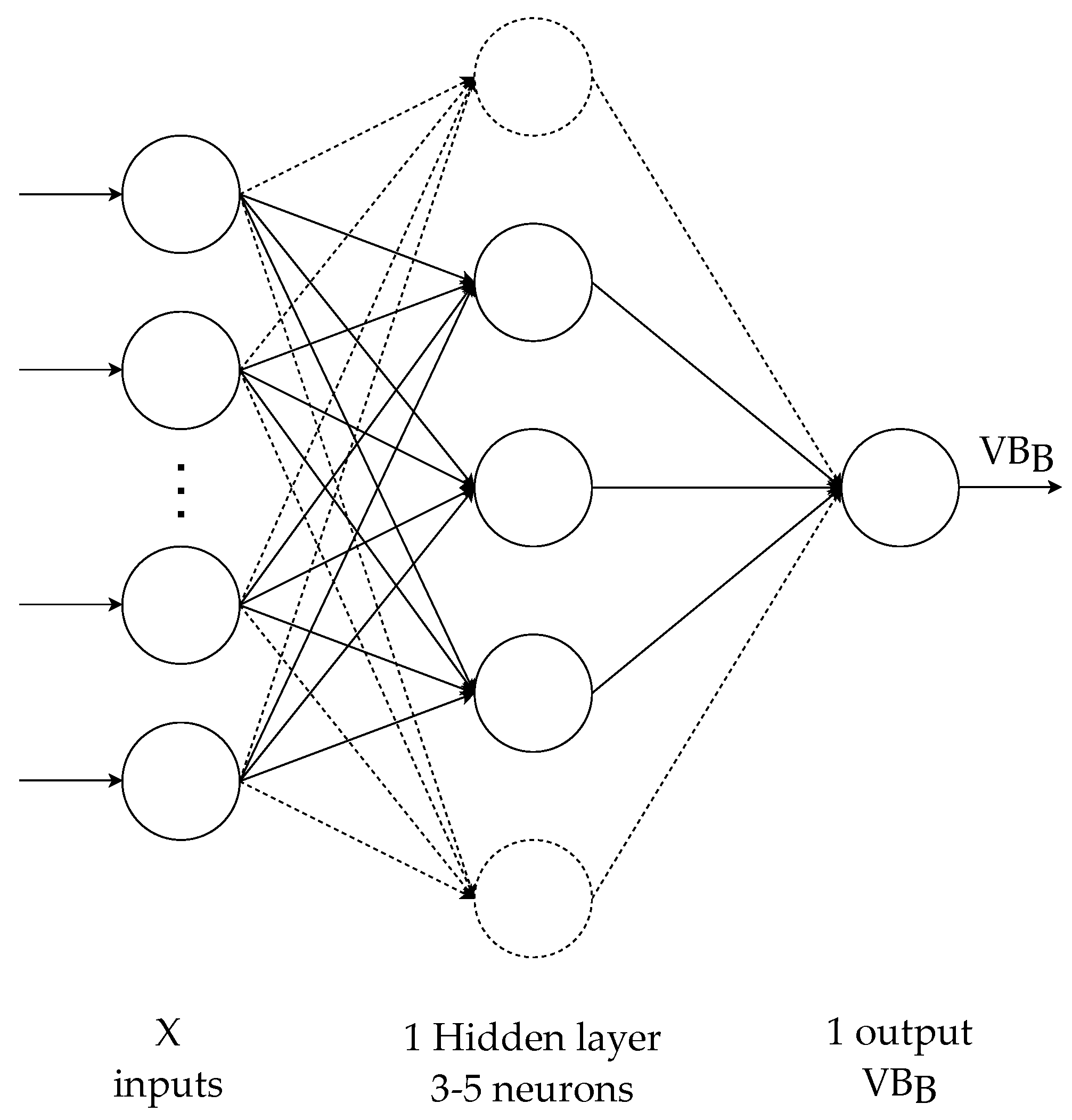
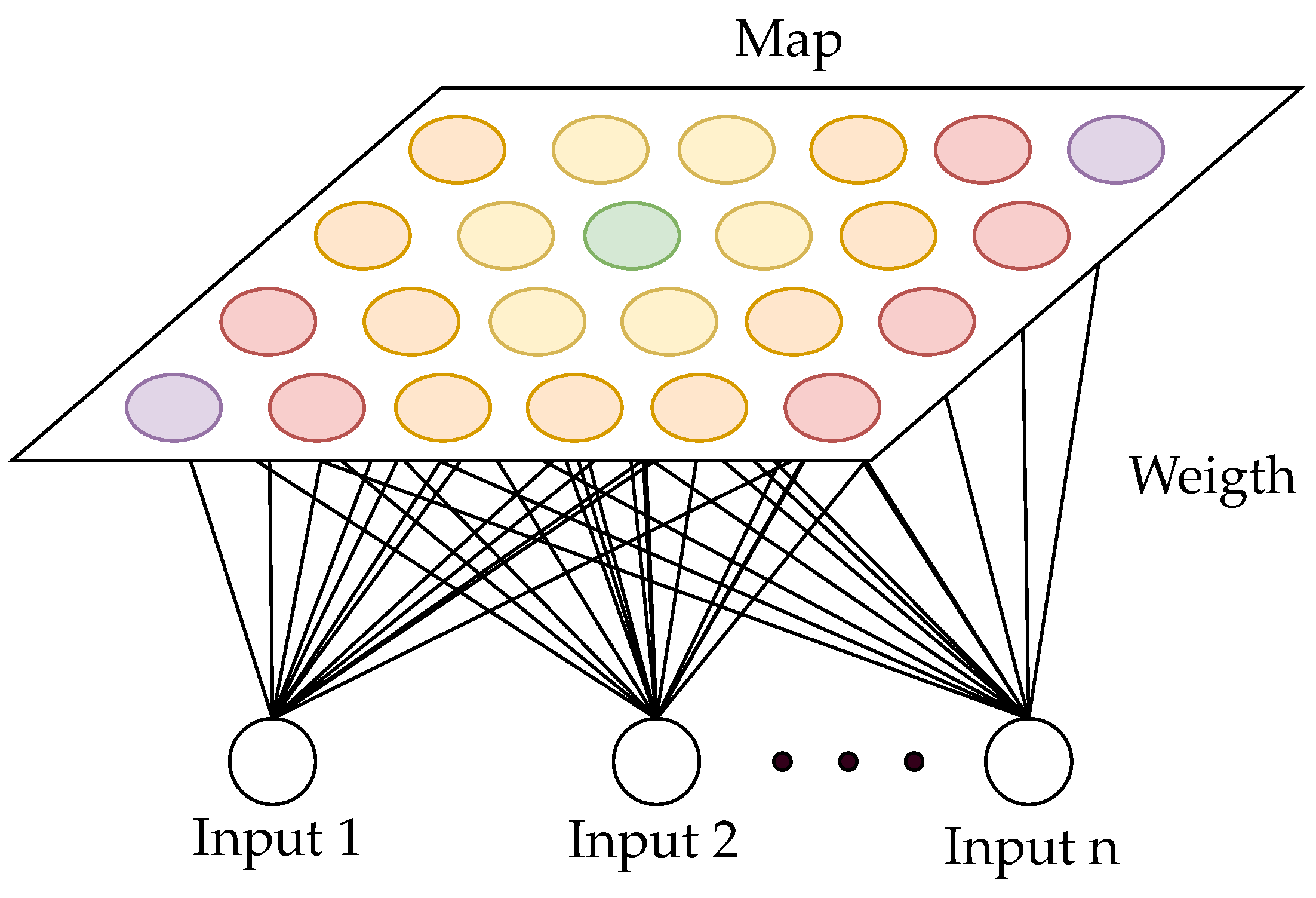
5.1.1. General Architecture of the Neural Network

The architecture of a neural network is often defined by trial and error and can have a major influence on the quality of the results. From the 44 papers about ANN, 17 propose an architecture with one hidden layer [33,41,46,52,53,54,55,56,57,58,59,60,61,62,63,64,65], two propose an architecture with two hidden layers [66,67] and the rest does not give any information about the network architecture. From these papers, the most common architecture of the neural network to monitor the tool wear is presented in Figure 8. This architecture is composed of three layers: one input layer, one hidden layer and one output layer. The number of neurons in the input layer depends on the data used as inputs. In the hidden layer, the number of neurons is around 3 to 5. Finally, the output layer is generally composed of one neuron that gives information about ${\mathrm{VB}}_B$ (Figure 8). This architecture therefore appears to be the most efficient to resolve the subject of this SLR. Apart from the network architecture, other considerations exist. An exhaustive comparison of different types of NN is presented in [68]. The influence of the optimizer is studying in [69,70]. A comparison between different architectures and activation functions is made in [55]. It is also worth noting that [71] proposes an approach based on a recurrent neural network.

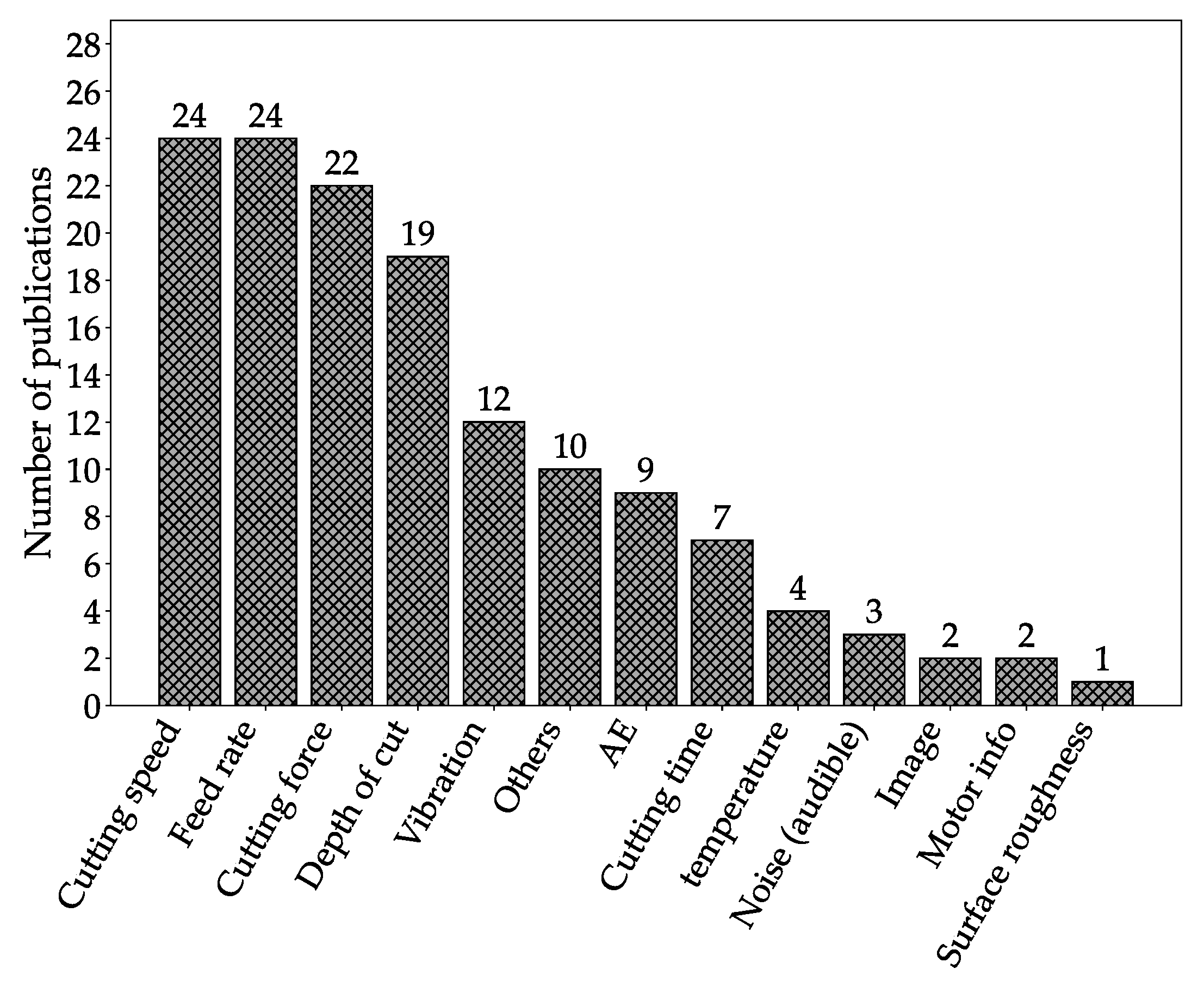
5.1.2. Input

The different features used as input of the neural network, based on the 44 articles on the subject, are presented in Figure 9. The six most used features are: cutting speed, cutting forces, feed, depth of cut, vibration and acoustic emission (AE). In these data, only three are dependent on the state of the tool: cutting forces, vibration and AE. The three others are cutting parameters that are necessary to help the neural network to identify the cutting conditions.

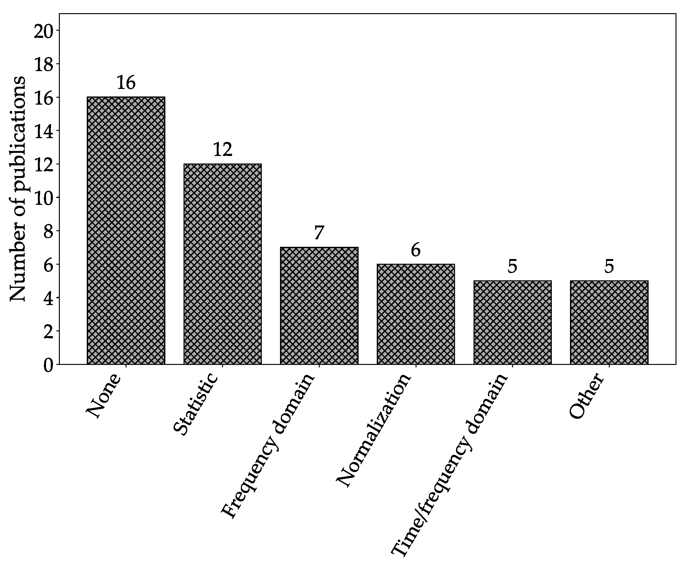
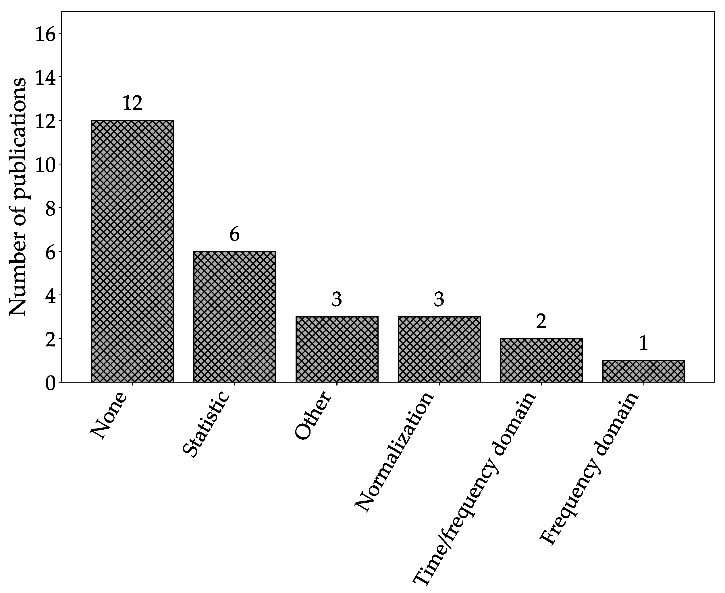
5.1.3. Pre-Processing

To extract useful information about these signals, pre-processing techniques are employed. Figure 10 shows the pre-processing techniques used in this context. As the two most used pre-processing techniques are: None and Statistic, it appears that, for ANN, complex techniques are not always required. When a pre-processing is applied, it is a very simple one that consists of computing the skewness, kurtosis, etc. Note that the category “None” refers to articles that do not present the pre-processing technique used. As some sort of pre-processing is always needed, it indicates that these articles only compute simple statistic value on the “raw” signal from the sensors such that it does not require extensive presentation of the pre-processing technique. This observation confirmed what is presented in Appendix B.1: ANN is robust to noisy data such that advanced pre-processing techniques are not needed for all the inputs.

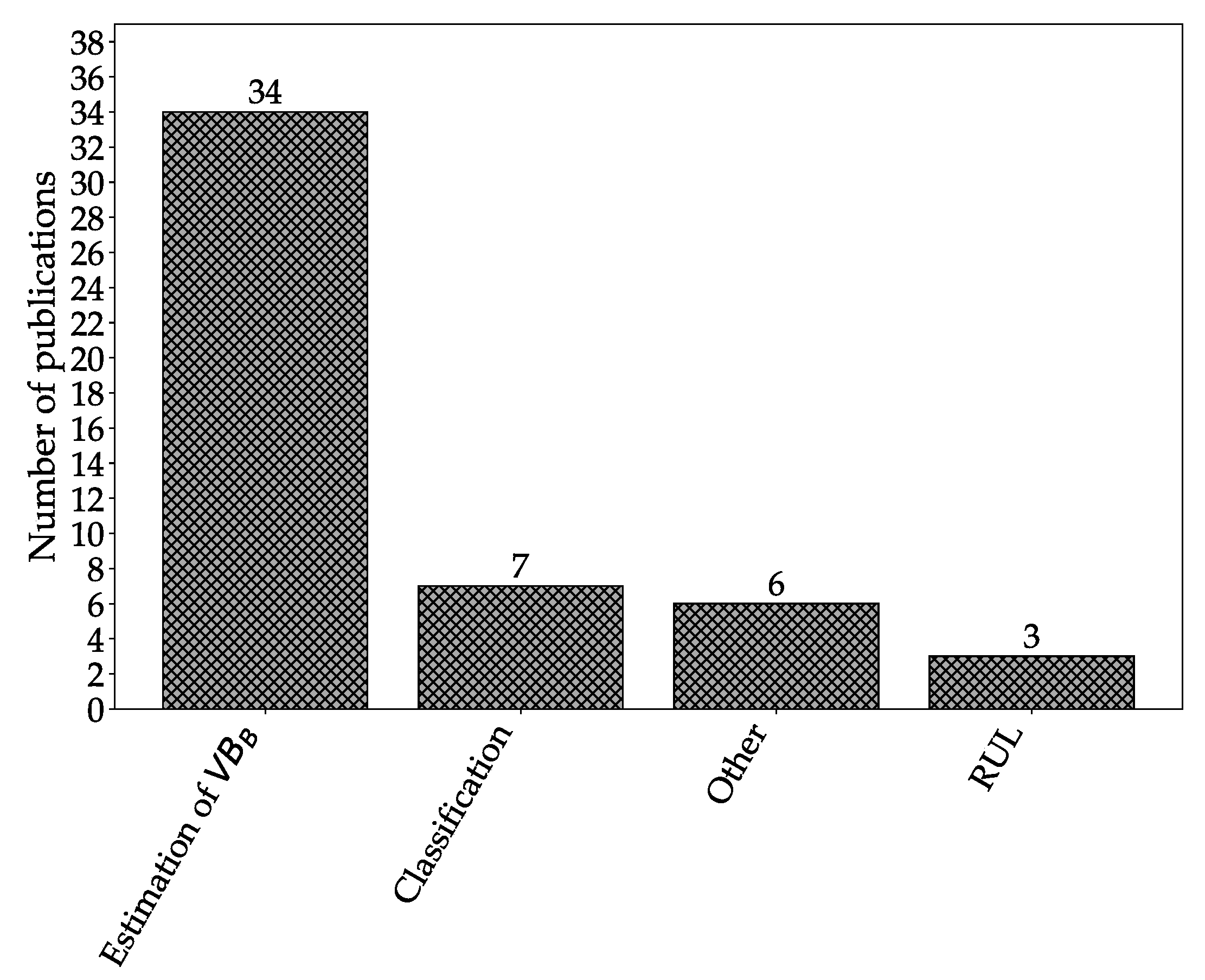
5.1.4. Output

The output of the neural network is presented in Figure 11. The vast majority of papers use the ANN as a regressor to estimate the value of ${\mathrm{VB}}_B$ in real time (“estimation of ${\mathrm{VB}}_B$” in Table A1 and Figure 11). Some papers also use the neural network as a classifier, and the classification is on average performed for three states. The RUL is used in [72,73] with the latter giving an upper and lower limit for its prediction. Some articles use a different approach: [57] monitors the percentage of tool life, [74] monitors the tool life and tool-shim interface temperature, [75] monitors the surface roughness to latter predict the flank wear and [59] monitors surface roughness and flank wear.

5.1.5. Comparison

Some articles present the results of the ANN by comparing its performance with those of classical regression methods [59,61,67,73,75,76,77]. Some of them also completely describe a regression method in their approach [59,61,67,75,76]. In all these papers, the observation is that ANN performs better than the classical regression methods. The advantage of ANN over the regression model is its ability to continuously learn from the data, making it more efficient at monitoring the tool wear.

5.1.6. Conclusions

The great interest in this technique can be explained by its history in the framework of tool monitoring. Indeed, before the year 2000, the majority of publications concerning the use of AI applied to cutting tools concerned the use of neural networks [10]. This can be explained by the ease of implementing neural networks and the great interest that this technique received among researchers. Today, many accessible libraries make it possible to code a neural network easily, e.g., in Python, TensorFlow [78] and Scikit-Learn [79] are two commonly used libraries. It is also well known that ANN are efficient to model highly nonlinear models which is our case of interest [80]. One of the major drawbacks of ANN is its “black box” aspect. In today industries, the explicability of AI is a subject of great interest [81,82] but, by the number of articles about ANN, it appears that this consideration is not an obstacle to the development of this approach.

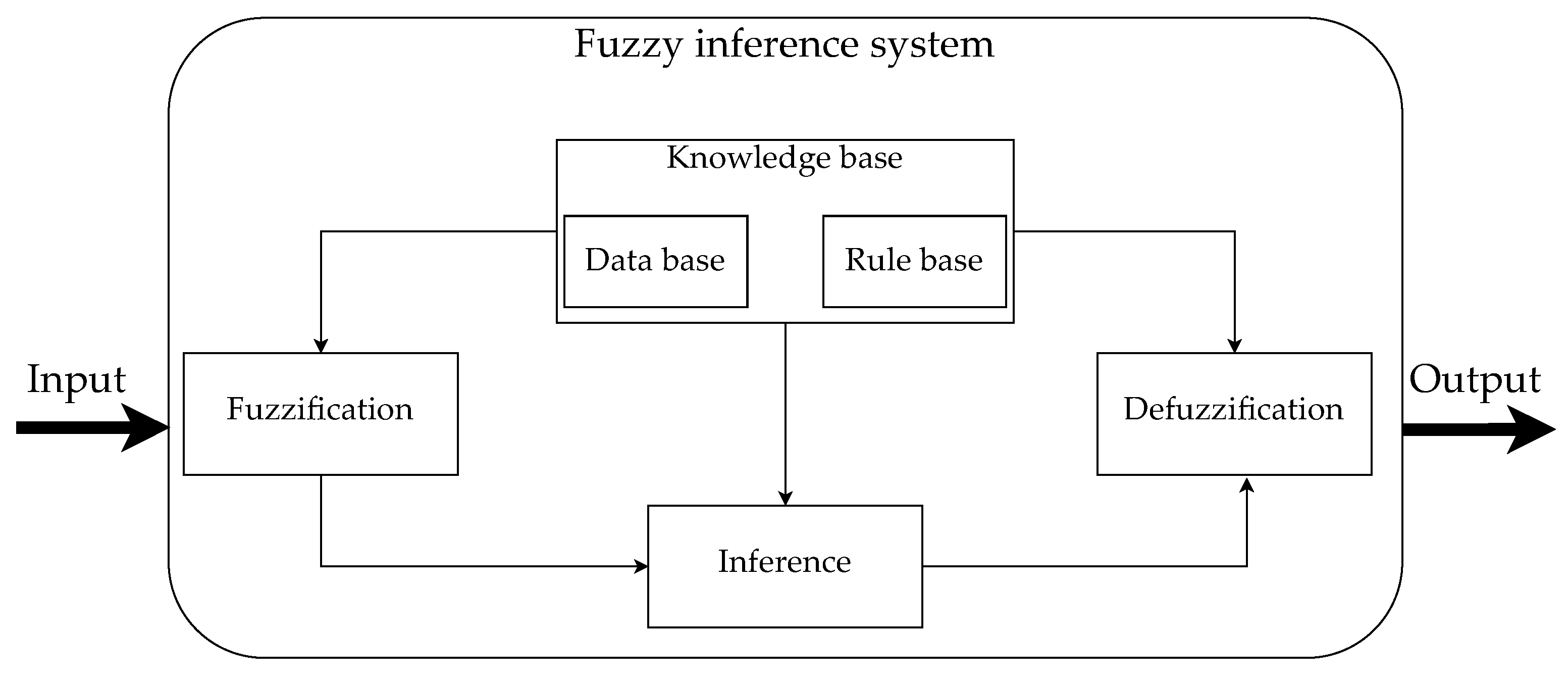
5.2. Fuzzy Inference System and ANFIS

This section presents the results for the ANFIS and FIS approaches. It was chosen to group these two approaches because the observations made in the following are identical for both. The 26 articles are presented in Table A2 for the FIS and Table A3 for the neuro-fuzzy approach.

5.2.1. Presentation of the Articles

There are 8 articles about FIS: [33,76,83,84,85,86,87,88] and 18 articles for the neuro-fuzzy approach: [33,36,37,41,58,89,90,91,92,93,94,95,96,97,98,99,100,101]. For the inference system, it is important to note that, out of the 8 articles, five articles have the author Balazinski Marek (and Baron Luc for four of these articles) in the author list which explains the similarity in the approaches presented in these articles ([33,84,86,87,88]).

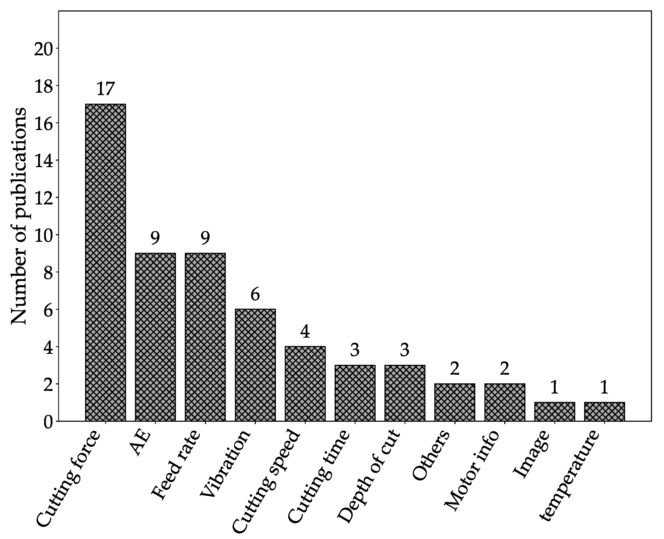
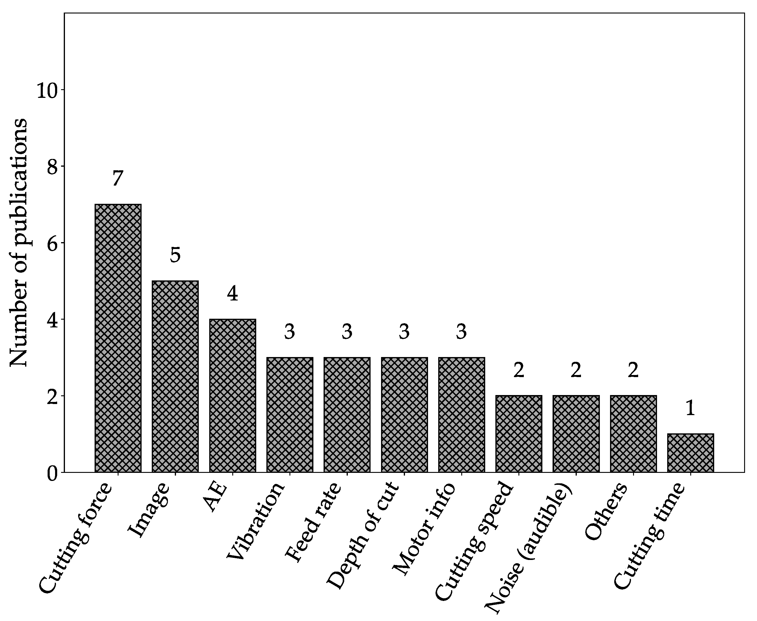
5.2.2. Input

The inputs used for the fuzzy models are presented in Figure 12. It is observed that the most used input is the cutting forces followed by the AE and feed rate signals. With 17 out of 26 articles using it, the cutting force is the most used input signal. A particular approach using temperature as well as the power and voltage of the machine as input signal is presented in [93].

5.2.3. Pre-Processing

The pre-processing technique use is presented in Figure 13. The most used pre-processing techniques are: None and Statistic. It indicates that the fuzzy logic approaches do not require elaborated pre-processing technique to obtain a good accuracy.

5.2.4. Output

The output of the fuzzy models is presented in Figure 14. The vast majority of articles use the fuzzy logic to monitor the flank wear ${\mathrm{VB}}_B$.

5.2.5. Comparison

For the FIS, the papers [86,87] perform a comparison of their approach that uses a Tagaki–Sugeno–Kang Fuzzy Approach Based on Subtractive Clustering Method with a neural network, neuro-fuzzy and Mamdani fuzzy logic. The approaches proposed in these papers have a lower root mean squared error on the prediction of ${\mathrm{VB}}_B$.

5.2.6. Conclusions

The fuzzy approaches occupied a large amount of the literature around the 2010s; today, they are much less represented in the literature. There is nothing that explain this decline in interest. It seems that the interest by the researcher has evolved such that these approaches have been replaced. The interest of fuzzy approaches lies mainly in their explicable aspect. Unlike neural networks, a fuzzy approach is not a black box. This is a great feature, especially in shop floor applications where the fuzzy approach can be of interest by providing more information than a simple prediction. In [41], the low processor time is also cited as a key feature of the fuzzy approach compared with neural networks.

5.3. SVM

As mentioned in Section 4.2, SVM received great interest over the past five years and is one of the most used techniques to monitor the tool wear with 18 articles. A presentation of these articles is provided in Table A4.

5.3.1. Input

The input features used for the SVM approach are presented in Figure 15. It is observed that the most used input is the cutting force. It also appears that the use of images to generate features is more commonly used in this AI technique than with other approaches (except CNN).

5.3.2. Pre-Processing

Due to the sensibility of SVM to noise and outliers, it appears that this approach requires more pre-processing on the data than ANN. Indeed as Figure 16 shows, the vast majority of the approaches show the use of a pre-processing technique. This pre-processing is performed in the time-frequency domain and some statistical features are computed.

5.3.3. Output

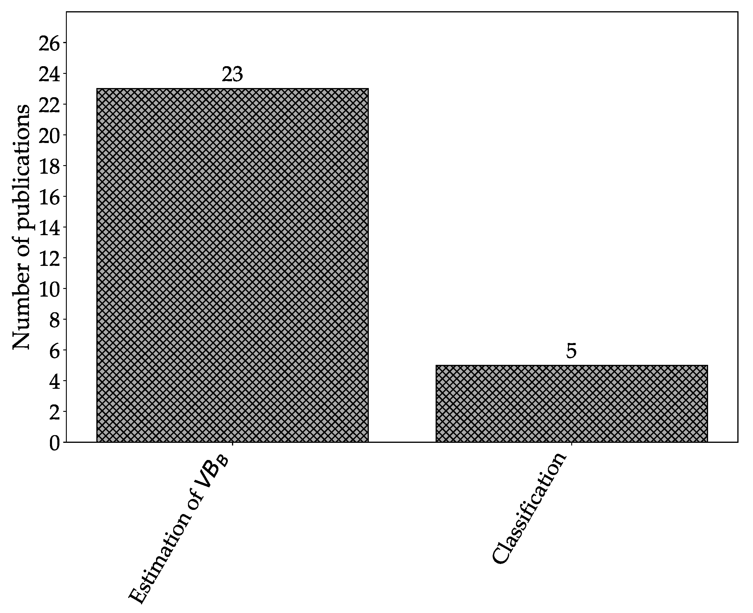
The output of the SVM is presented in Figure 17. As described, SVM was initially only used in classification purpose. Here, the number of articles that use SVM for regression and classification are almost the same.

5.3.4. Comparison and Particular Approaches

In a particular article [102], the authors use the SVM approach to make a short-term prediction of ${\mathrm{VB}}_B$ at time t and also at time $t+1$ (“prediction of ${\mathrm{VB}}_B$”). This approach uses SVM coupled with a genetic algorithm to perform this task. A comparison is realized with an AutoRegressive Integrated Moving Average (ARIMA) model and the SVM approach developed in that paper. The authors demonstrate that the SVM approach performs better than the ARIMA model.

In another instance, it is proposed to use the cutting forces to classify the state of the tool into three states (“initial”, “normal” and “severe” wear) [103]. The cutting forces are pre-processed with several techniques: normalization, statistical features and time-frequency domain. This is followed by a correlation analysis to find the best features. These features are used as input of a Gravitational Search Algorithm–Least Square Support Vector Machine model (GSA-LSSVM). In this entry, the authors compare the results obtained with this technique with other related methods such as: K-Nearest Neighbour(k-NN), Feed Forward Neural Network (FFNN), Classification And Regression Tree (CART) and Linear Discriminant Analysis (LDA). The classification obtained with the GSA-LSSVM model outperforms the others. However, most other authors using SVM in this context compare SVM with ANN, and they show that SVM is more accurate (in classification and regression) than ANN [31,104,105,106]. Some authors also compare the results obtained with SVM and other AI techniques: [31,103,104,105,106].

5.3.5. Conclusions

Applications of SVM appeared later in the literature and remain a relatively modern approach. As this method is more dependent on the quality of the input data, some feature extraction is required to improve the quality of the inference. Fitting the correct parameter in the SVM approach is a complex task, but it appears that the quality of the inference made with this approach is at least at the same level as with an ANN approach. In practice, this method may be more difficult to implement in the industrial sector due to its sensibility to noisy data, and it needs a pre-processing approach. However, SVM has the advantage of a good generalization performance which could make this approach particularly interesting in the future.

5.4. SOM

Only 7 articles described this approach and are presented in Table A5.

5.4.1. Input

The inputs of the SOM are presented in Figure 18. Due to the nature of this approach, only inputs that are highly correlated with the tool wear are used. Indeed, the cutting parameters such as cutting speed, depth of cut, feed rate, etc. are not used as input of the SOM contrary to other approaches.

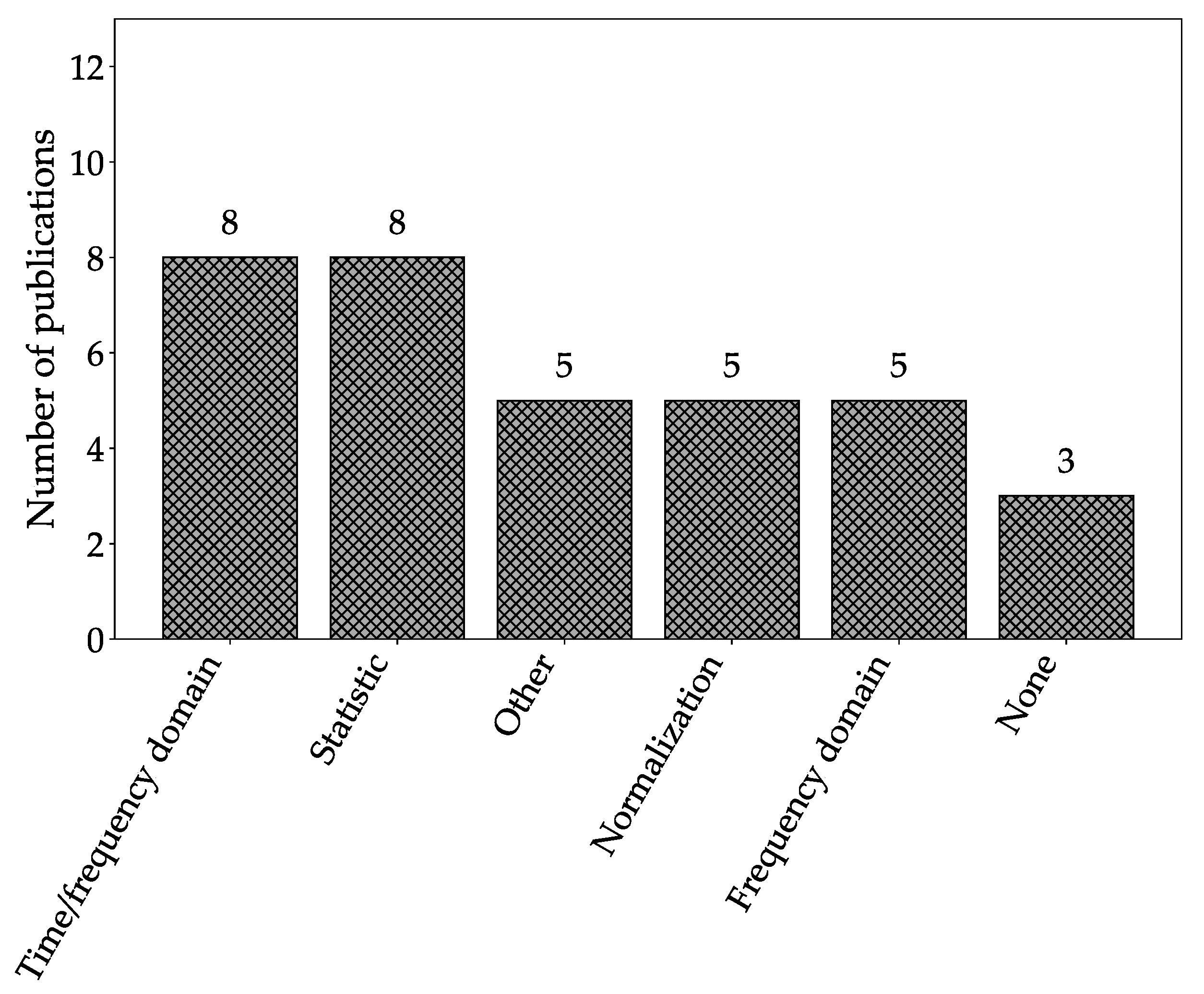
5.4.2. Pre-Processing

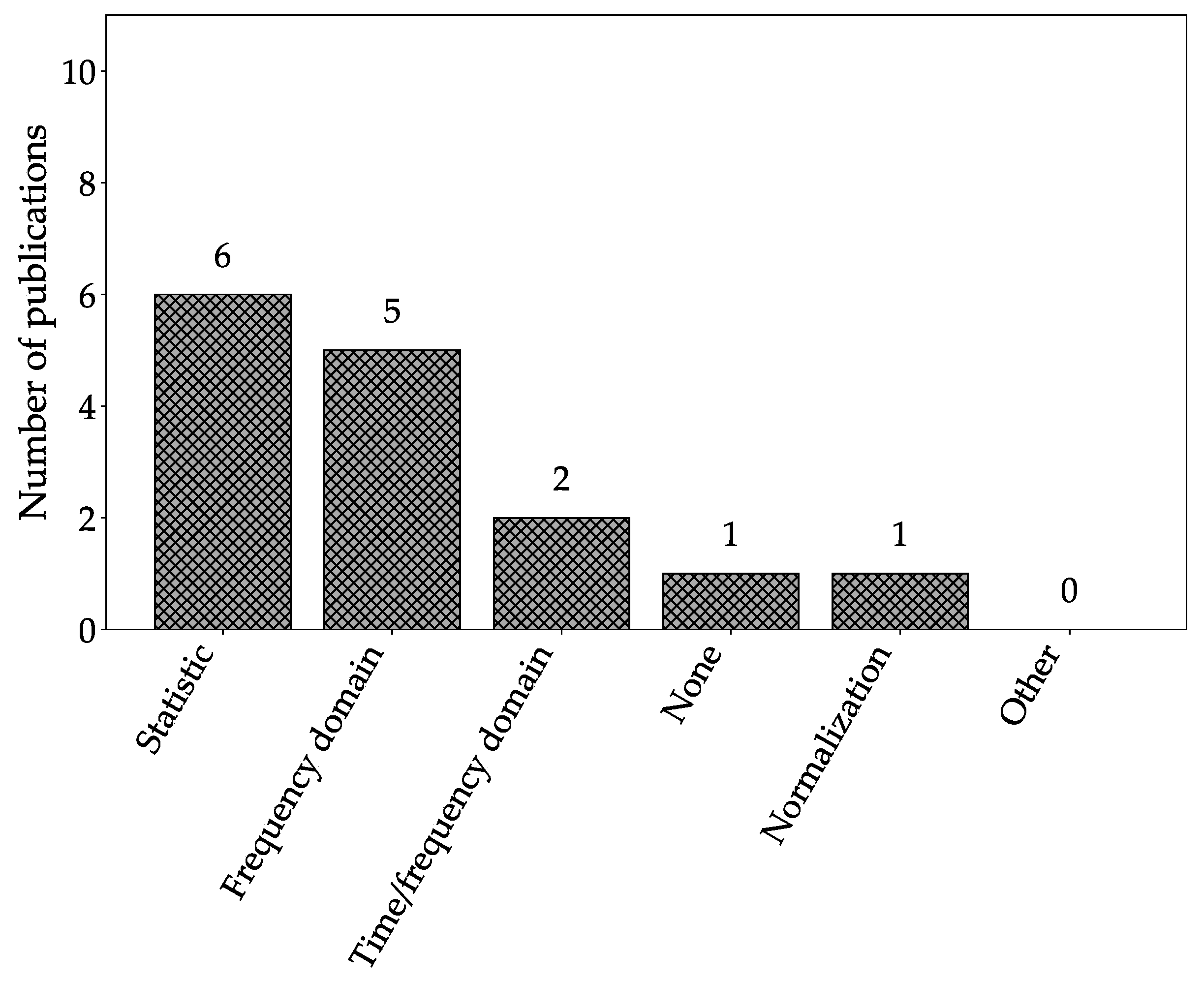
The pre-processing techniques used are presented in Figure 19. It is observed that the statistical features and frequency domain features are the most used pre-processing approaches. As presented in Appendix B.4, this method is generally robust against noisy data but computing the kurtosis, skewness, average value, etc. is an easily accessible way of improving the results obtained with this approach and reducing the learning time.

5.4.3. Output

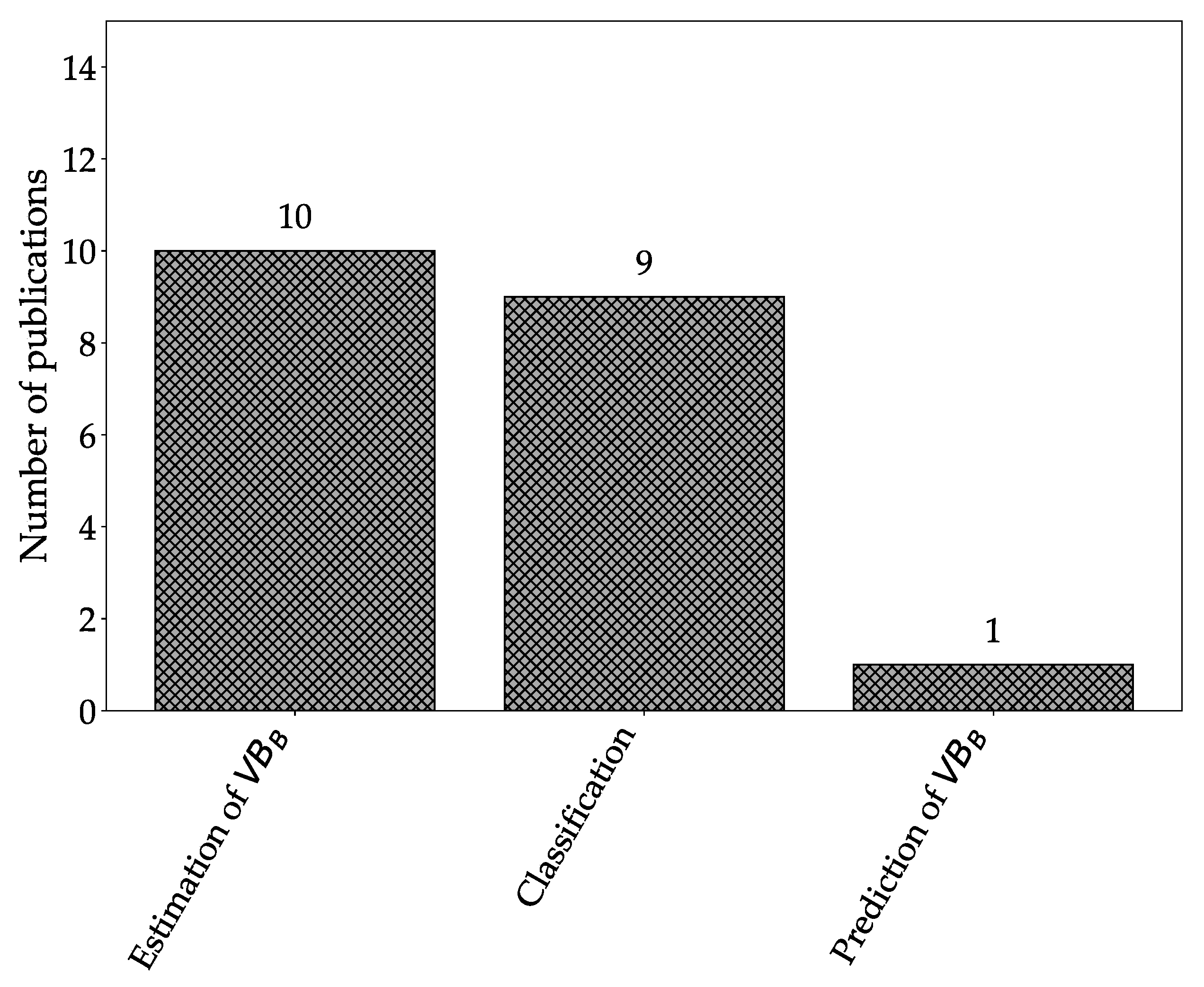
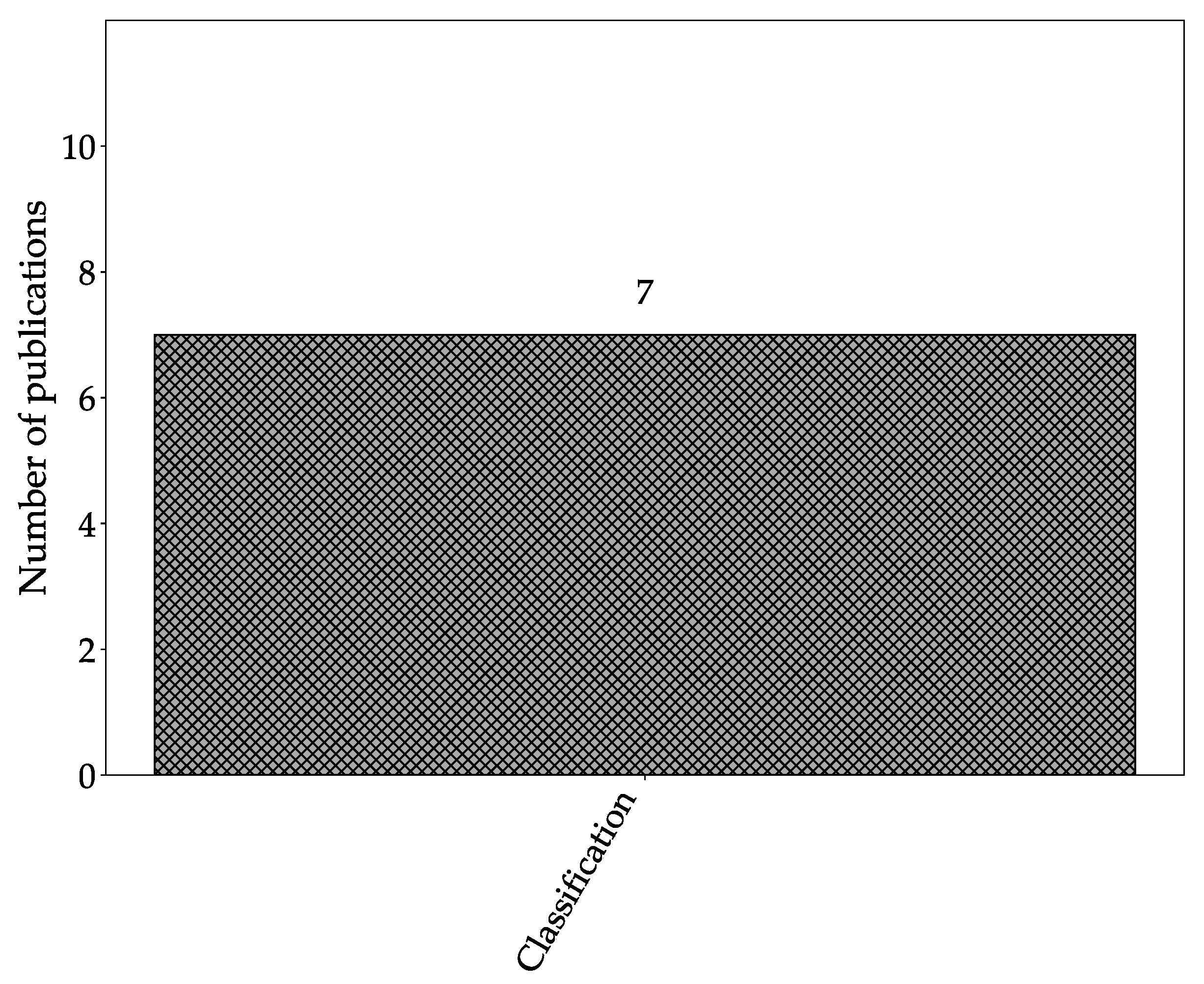
This approach is only able to perform classification as observed in Figure 20.

5.4.4. Comparison

Some articles present the SOM with another method. In [2], a comparison between SOM, SVM and k-nearest neighbour approach is realized. In [41], the use of SOM, neuro-fuzzy and ANN is discussed and software is presented for shop-floor application. In general, the SOM approach does not outperform the others but proposes a simple and accessible classification solution. However, the lack of generalization capabilities of this approach requires training under all cutting conditions, which is not always necessary with other methods.

5.4.5. Conclusions

The SOM approach is quite different from the others by its unsupervised learning aspect. Some authors use this aspect to try to select the best features independently of classical correlation approaches [107]. Other uses this aspect to work with imbalanced data and uni-sensor approach [2]. In an industrial application, imbalanced data often constitute the only available data, and this technique can therefore be used in this context. The advantage of low computation time is also highlighted [41].

5.5. HMM

The HMM approach is not strongly represented in the literature with only 3 articles: [32,46,47]. These articles are presented in Table A6. They are all used to perform a classification on the tool state.

5.5.1. Presentation of the Articles

In Ref. [32], a discrete hidden model uses the wavelet transformation on the vibration signal in the feed direction to classify the tool state within two states (“sharp” or “worn” tool). This approach achieves a hit rate up to 97%. The authors try this approach under different training conditions (e.g., length of training data and variation of observation sequence length), and the HMM performs well in all conditions.

In Ref. [47], a Discrete Hidden Markov Model (DHMM) is used in combination with an SOM. They use the cutting force and the acceleration to monitor the state of the tool and these features are pre-processed with a FFT and coded with a SOM. Their approach performed well, and a processing time of around 0.2 s is reported, which makes this approach usable in online applications.

In Ref. [46], the use of ANN is compared to an HMM to monitor the tool wear. The cutting force signal is used as input, pre-processed with multiple techniques: statistical (mean, skewness, etc.), frequency (FFT, PSD) and time-frequency (wavelet and spectrogram). The best features are chosen by the researcher following a correlation analysis. It is concluded that both approaches perform well with the advantage of HMM to be extremely easy to train but limited to a certain amount of output values (classification).

5.5.2. Conclusions

Even if this approach presents only 3 papers in the literature, the results reported in these publications show that this technique is capable of realizing a good quality classification. In theory, there are Markov models capable of performing a regression, but these have not been tested yet in the literature. As the classification of the tool state is not the most common approach, the low interest in this technique can be explained by this consideration. Moreover, as stated in one of these articles, in comparison, a neural network is able to have the same precision as an HMM. However, the neural network needs a little more trial and error to determine the best architecture for learning [46]. HMM therefore does not seem to present any major advantages, which leads researchers to not favour this approach over another.

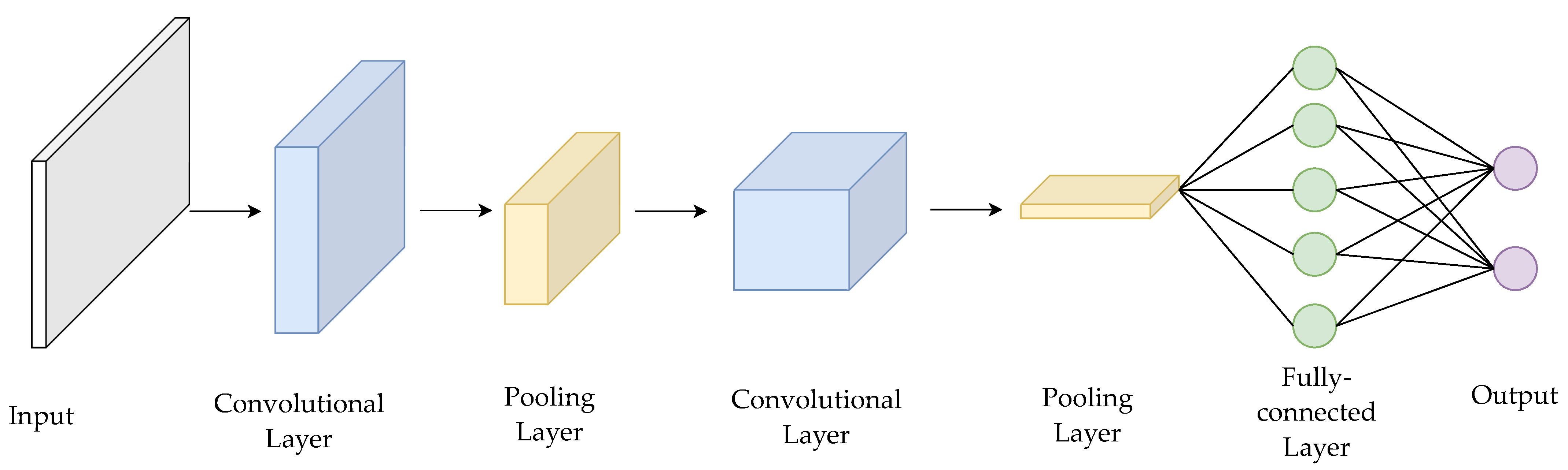
5.6. CNN

The use of CNN has recently emerged. Only 3 articles discuss the use of CNN to monitor the tool wear: [9,48,49]. They are presented in Table A7. All of these articles have been published in 2020 showing a new interest in this techniques (see Section 4.2). These articles almost use the same approach.

5.6.1. Presentation of the Articles

In [49], the authors used the image of the insert to compute the value of ${\mathrm{VB}}_B$. This is achieved by identifying the wear area on the tool. The identification of this zone makes it possible to count the number of pixels which allows finding the dimensions of the wear zone. The authors perform a data augmentation on the initial dataset to improve the robustness of the CNN. In [9], a similar approach is followed, but the images of the insert are used directly to classify the state of the tool. In this study, the classification is made within two classes: “GO/NO GO”. Both articles report accuracy greater than 90%.

Based on the dependency of chip colour on the cutting tool temperature, and the influence of tool wear on tool temperature, it has been proposed to use the chip colour to monitor the tool wear [48]. Images of the chip are pre-processed to remove the background and a kernel density estimation is performed. They show that this density estimation is more efficient on the hue channel from the Hue Saturation Value (HSV) channels of the images. This is used as an input of the CNN which performs a classification around three classes depending on the class of the wear: “New”, “Medium” and “High”. They achieve accuracy of above 90%. A comparison is made with a functional data analysis (FDA) classifier, and it fails to beat the CNN.

5.6.2. Conclusions

The late interest in this technique can be explained by the complexity to obtain a significant number of images for the datasets. Indeed, this technique uses images of the tool which can be impractical to obtain in industrial applications. These approaches work greatly in laboratory conditions but still require human intervention to achieve them. Comparing this approach with the others presented in this paper, automating this approach seems more difficult. In addition, in real production applications, turning is often performed with cutting fluids which can further complicate image capture. Indeed, the conditions for taking images must be consistent and the light must be controlled so as not to influence the neural networks [48]. Today, to our knowledge, there is no automated machine allowing the introduction of a capture system of this type which may explain the low interest raised by this technique. This lack of interest can also be explained by the false belief that CNN is more difficult to implement than ANN [108]. Furthermore, this approach requires stopping the machining process to allow the picture to be taken which removes all the interest of monitoring in real time. However, the advantage of this approach is that it makes it possible to directly measure the wear on the tool rather than going through correlated indicators such as the cutting forces, for example. Automating this approach would be equivalent to automating the measurement of ${\mathrm{VB}}_B$, which would provide important data for other forecasting techniques. By using the chip colour instead, it could then be possible to carry out the measurement without interrupting the process [48].

5.7. Other

This section covers all approaches that are not related to the other categories. The articles are presented in Table A8. It can be noted that, among these methods, there is a majority of decision trees and classifiers. These approaches are generally compared in pairs with others, hence they do not have a dedicated section in this SLR.

5.8. General Conclusions

Table 3. Comparison of the three most used: input, pre-processing and output for each approaches.

	ANN	ANFIS & FIS	SVM	SOM	HMM	CNN
Nb of articles	44	18 & 8	18	7	3	3
Input	Cutting Speed (24)	Cutting Force (17)	Cutting Force (7)	Vibration (6)	Cutting Force (2)	Image(3)
	Feed rate (24)	AE (9)	Image (5)	Cutting force (5)	Vibration (2)	/
	Cutting force (22)	Feed rate (9)	AE (4)	Noise (2)	/	/
Pre-processing	None (16)	None (12)	Time-frequency (8)	Statistic (6)	Time-frequency (2)	Image processing (3)
	Statistic (12)	Statistic (6)	Statistic (8)	Frequency domain (5)	Frequency (2)	/
	Frequency domain (7)	Other (3)	Other (5)	Time-frequency (2)	Normalization (1)	/
Output	Estimation of ${\mathrm{VB}}_B$ (34)	Estimation of ${\mathrm{VB}}_B$ (23)	Estimation of ${\mathrm{VB}}_B$ (10)	Classification (7)	Classification (3)	Classification (2)
	Classification (7)	Classification (5)	Classification (9)	/	Estimation of ${\mathrm{VB}}_B$ (1)	Estimation of ${\mathrm{VB}}_B$ (1)
	Other (6)	/	Prediction of ${\mathrm{VB}}_B$ (1)	/	/	/

summarizes the top 3 inputs, pre-processing, and outputs for each AI techniques. From this table, the different methods are compared.

For ANN, 2 of the 3 most used inputs are cutting parameters: cutting speed and feed rate. This extensive use of cutting parameters as input signal appears to be specific to ANN as this characteristic is not observed for other methods. All AI techniques extensively use the cutting force as input signal as it is present in the top 3 of each AI technique (except CNN). Vibration and AE signal are also commonly used. It is worth noting that, except for CNN, SVM is the second method that uses features extracted from images as input.

ANN and ANFIS/FIS techniques do not appear to require elaborate pre-processing as most of the articles do not specify the pre-processing techniques employed (“None” in Table 3). SVM, SOM, HMM and CNN all require special attention to the feature extraction techniques, especially SVM and HMM, which benefit from more advanced pre-processing techniques in the time-frequency domain. For the majority of methods, the computation of simple statistic characteristic on the signal is commonly used. By its nature, CNN does not require the same kind of pre-processing technique as it mainly uses images as input.

Two outputs are predominant in the use of AI techniques: estimation of ${\mathrm{VB}}_B$ and classification. In the analysis of AI technique by year (Section 4.1), it was shown that ANN, fuzzy and SVM techniques are predominant in the literature. It is observed that these three techniques are the only ones with “Estimation of ${\mathrm{VB}}_B$” as the most represented output. Indeed, approaches such as SOM, HMM and CNN are mainly focused on classification. It is therefore observed that techniques monitoring the value of ${\mathrm{VB}}_B$ are favoured over a simple classification purpose.

As it is discussed in Section 6, comparing AI methods on the results they are able to achieve is not possible. Since each approach is carried out on a different dataset, with different indicators, with different inputs, etc. comparing these results would not provide a clear and unbiased analysis of the literature. Despite this fact, it is described in the previous sections that articles that compare the AI techniques with classical methods such as statistical model, show that the AI techniques outperform the classical models.

6. Discussion

As indicated by the various authors of the identified publications, all approaches presented in this SLR were able to obtain good results in monitoring the cutting tool health, some authors were even able to obtain more than 90% accuracy. The majority of these approaches have the common point to monitor the value of ${\mathrm{VB}}_B$ to assess the tool state. Unfortunately, there are few other approaches that try to evaluate the tool health differently. Some papers try to monitor the tool wear with other indicators such as its percentage of elapsed tool life, and others try to predict the RUL. This lack of other approaches may come from the difficulty to define a clear end-of-life criterion to cutting tools. In the ISO 3685 standard [19], the maximum value for ${\mathrm{VB}}_B$ is set to 0.3 mm as the end-of-life criterion, but, in real application, this value may not represent the cutting tool end-of-life, depending on the industrial applications and its tolerances. As this end-of-life can be very variable, having approaches based on the RUL or other time indicator can be very difficult to adopt for industrial applications. It is therefore understandable why researchers are more interested in the value of ${\mathrm{VB}}_B$ rather than trying to define a precise end-of-life criterion. It is up to the AI user to define the criteria corresponding to its application. By proposing an approach that monitors ${\mathrm{VB}}_B$, the researchers ensure that their method can be applicable in real applications.

Knowing the current condition of a tool is obviously of great interest in condition monitoring. However, as the industry evolves, predictive monitoring tends to be the preferred approach. The current state of the art shows that there is too little research done to meet the future needs of industries in predictive maintenance, i.e., to predict the coming evolution of the tool condition. In recent years, advanced statistical models tend to answer this problem but still require a lot of tuning to obtain results. The use of AI could perhaps meet these needs of industries while guaranteeing models robust enough to be implemented on shop-floor applications. At this stage, it is not possible to assess whether this lack of interest in predictive maintenance is due to a lack of interest from the researchers or if it comes from a publication bias. Indeed, in this SLR are only listed articles that present relatively good results, and this may either be due to the fact that all techniques were always able to perform well, or that the publications which do not get good results are not published or not submitted for publication. It is therefore possible that, currently, research in predictive maintenance is not published due to a possible lack of results.

Due to the different nature of the AI techniques, it is not possible to make a comparison between each of them. Many articles compare their approach with other methods. In this SLR, these articles are listed and their results presented, although they are often contradictory. Indeed, an approach presented in any of the selected articles is often presented to be the most effective compared with others. Given these contradictions, it is impossible to identify the best approach, if one exists. This may come from two reasons: (i) the publication bias previously discussed (the papers are not submitted or published if their approach is not better than another one), (ii) there is no best approach. Moreover, out of 102 articles, 98 performed a test campaign to obtain their dataset. As these data have been collected with different cutting conditions, materials, tools, … it is not relevant to compare the results of these approaches. In turning, there is no benchmark dataset allowing for fairly comparing all the approaches, whereas benchmarks exist for other categories of machining. In milling, for example, some datasets are available on the NASA website [109], on the PHM website [110], … This lack of unified benchmarking in turning does not allow a clear view of the performance and is a clear limitation of the comparison of performances in all these articles, which can therefore only be analysed objectively on the bases of their methodology instead of their results. The results obtained are therefore highly dependent on the quality of the data recovered during the tests and some data may be more fitted to certain approaches than others. Consequently, the pooling of various test data would allow the establishment of benchmarks. These benchmarks should aim to be the most representative of industrial reality. This lack of unified dataset can also be in relation with the co-authorship analysis performed in Section 4.5: as there is little inter-laboratory collaboration in the topic of this SLR, no data are shared between researchers.

It is also observed that the title of the articles could be confusing. Indeed, many articles incorrectly used the word “prediction” to talk about “monitoring”. As a matter of fact, out of the 102 identified articles, 34 wrongly use the word “prediction” in their title and 62 in their title or abstract. The word prediction, in the English language, normally evokes the future state as defined in the Oxford dictionary: “Prediction is a statement that says what you think will happen” [22]. As shown in this SLR, the majority of articles actually use the AI technique as a monitoring system (i.e., to produce an estimate in real time). There is no forecasting of the future state. This abuse of language likely leads to confusion given the previous remark on the emergence of predictive maintenance.

7. Answers to the Research Questions

This section presents an answer to the research questions identified in Section 3.1. The answers to these questions are distributed through this SLR, but the main results are summarized here.

RQ1 

How is AI used in the framework of monitoring/predicting the condition of tools in stable turning condition?

This question is answered throughout this SLR and RQ2 to RQ5. Several approaches have been mentioned and there is not one that stands out from the others (mainly due to the lack of unified benchmark). Each approach can find its place depending on the means and equipment made available to the monitoring system. However, as discussed in Section 6, it appears that, in the current state of the art, too few papers concern the evolution of ${\mathrm{VB}}_B$, as they rather monitor the current state of the tool, which could be a problem in the framework of predictive maintenance in industry 4.0.

RQ2 

What are the most used AI techniques used in this context?

In Section 5 of this SLR, all the AI methods were presented. Among them, there does not appear to be a more efficient approach than another. Each approach has its advantages and disadvantages. However, it appears in Section 4.2 that approaches from neural networks, fuzzy logic and support vector machines are particularly present in the literature. They all have the ability to be integrated into workshops. Neural network approaches have the advantage of having been widely studied but have a “black box” aspect which could cause reluctance in practice. Fuzzy logic seems to no longer be considered even though they had the advantage of presenting the results in an easily understandable way. In addition, finally, SVM approaches seem to perform as good as ANN and fuzzy approaches but require special attention to data pre-processing and the choice of parameters.

RQ3 

What is the forecasting horizon of each of the identified AI techniques in this context?

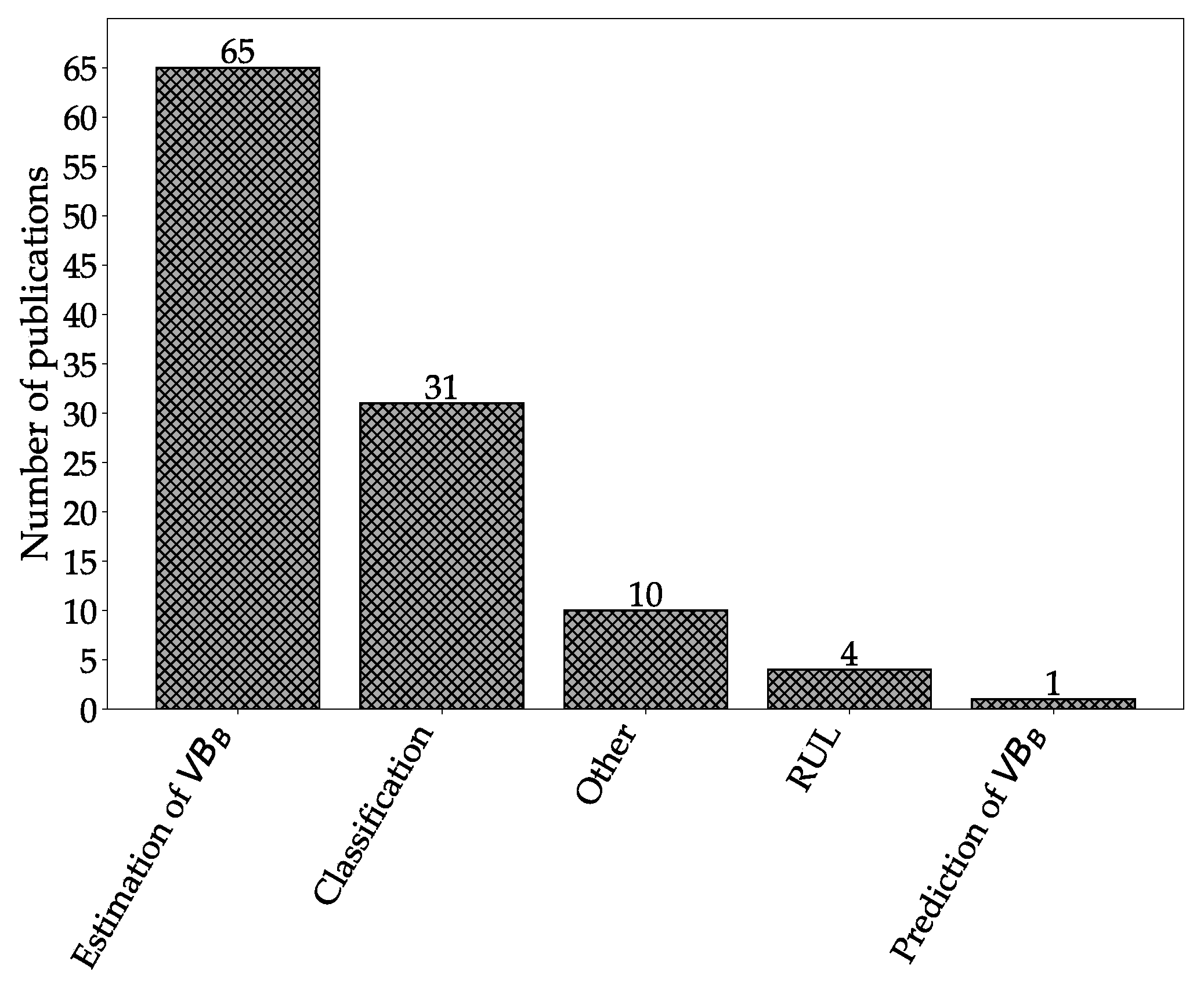
Figure 21 presents the outputs of all the AI techniques presented in this article. It appears that the majority of articles use AI to monitor the current state of tool wear (estimation of ${\mathrm{VB}}_B$). A classification purpose is also realised to detect the actual state of the tool. Some papers also present other kinds of output such as the percentage of tool life. Only five articles propose an approach that consist of a prediction of the future state. This is achieved by computing the remaining useful life (RUL) or a prediction of ${\mathrm{VB}}_B$ at a future time (generally called “$t+1$”). As discussed in Section 6, there is a lack of application in predictive maintenance and the actual state of the art is limited to the actual monitoring of the tool.

RQ4 

What are the most common inputs used with the different identified AI techniques in this context?

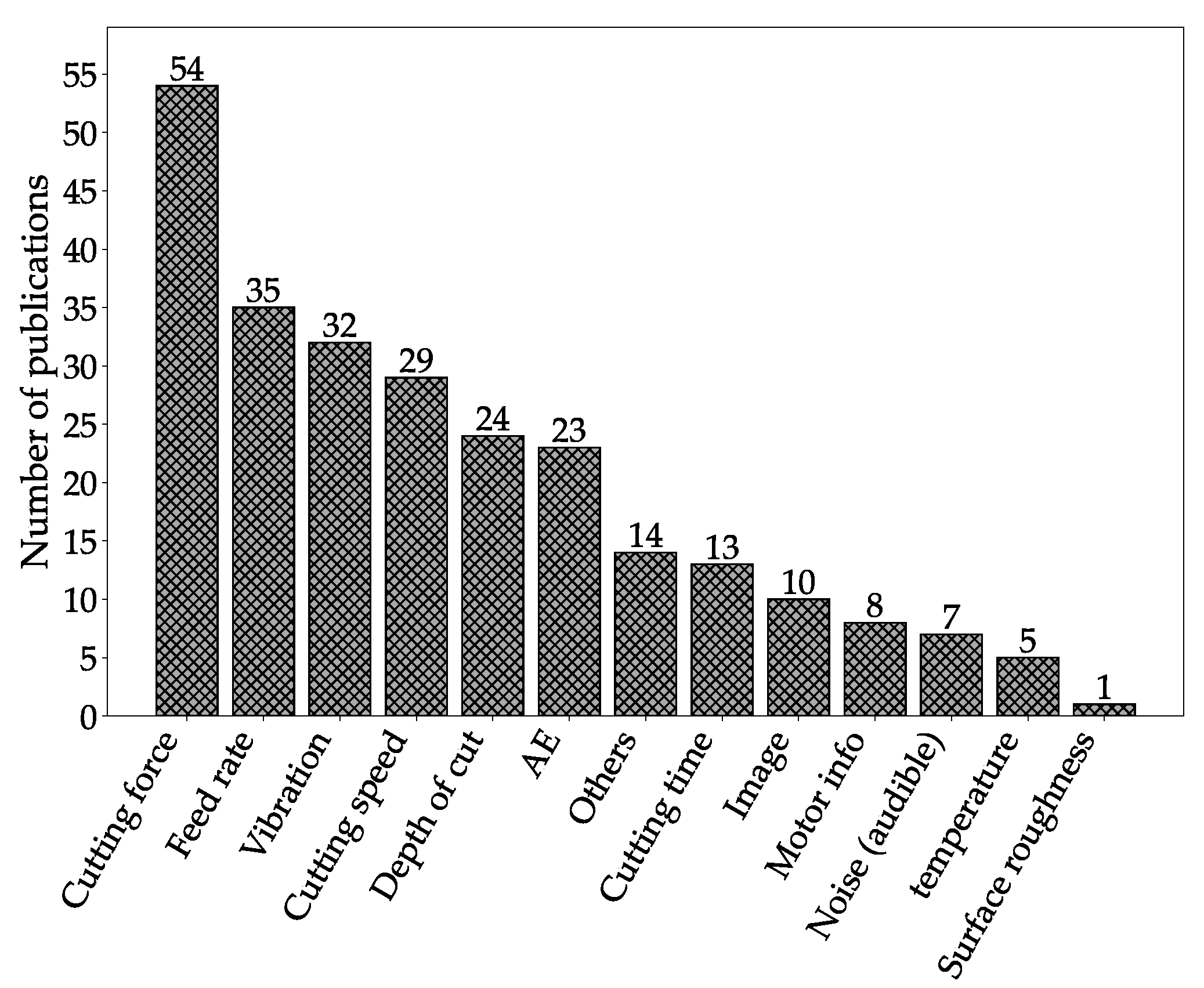
As AI techniques are data-driven, the most common features have a high correlation with the cutting tool state. The repartition of all input data for all techniques is presented in Figure 22. The cutting force is the main input as it appears in 54 of the 102 articles. Features that correspond to the cutting conditions such as: feed rate, cutting speed, and depth of cut are also used a lot. These features are generally constant through the cutting process but are important to give context to the correlated data such as the cutting force, vibration signal, … These cutting parameters thus have a significant impact in the ability of the AI technique to perform the monitoring of the tool.

RQ5 

What are the most used features extraction techniques in this context?

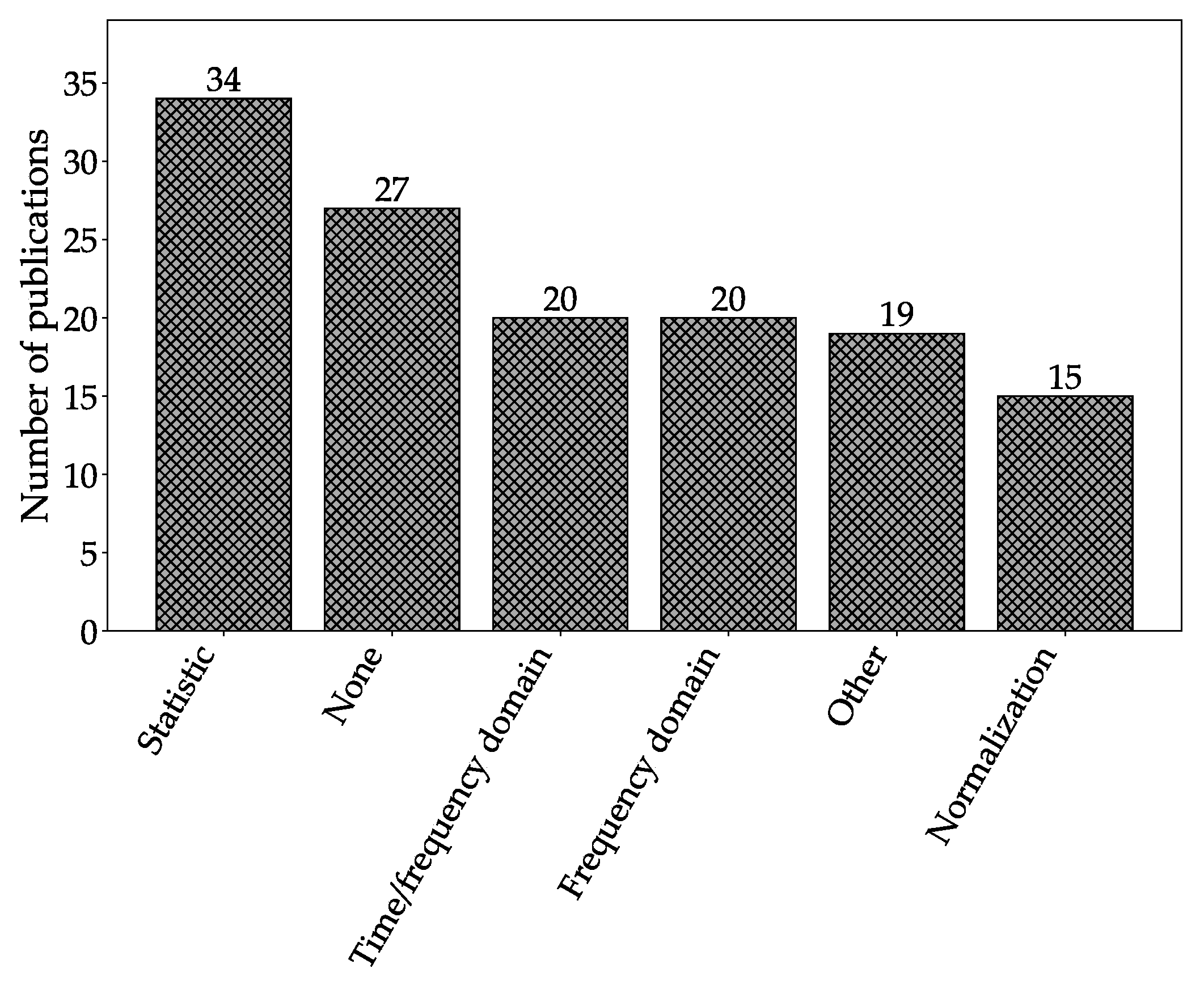
The features extraction technique for each AI approach is presented in Section 5. Figure 23 presents the repartition of all pre-processing techniques in this SLR. It is important to note that, depending on the approach, the pre-processing technique can be different. For example, it is observed that using ANN does not need much pre-processing while, for SVM, the pre-processing technique is necessary.

8. Conclusions

This paper presents a systematic literature review covering the use of AI techniques in the monitoring of cutting tool health in stable turning condition. The review protocol allowed for identifying 8426 articles in which 102 articles are corresponding to criteria of interest (Section 3). The review protocol followed the procedure recommended by Kitchenham [15]. During the definition of the research procedure, a new approach that aims to improve the quality of it was proposed. Some conclusions can be made about them:

• In the research procedure for this SLR, the choice to use a semantic approach to build the keywords was successful. It was chosen to construct each search query with a combination of four keywords so that each correspond to one part of the semantic approach (Section 3.2.2). The results show that this approach allows for browsing all of the literature on the subject of interest. However, it needs some additional sorting steps such as removing the “duplicated” items. Due to the number of articles identified, this last step cannot be performed manually. This approach is particularly interesting in the context of a systematic literature review.
• In the research procedure, to evaluate the inter-rater reliability, the Cohen’s kappa [30] was used to evaluate the agreement among raters (Section 3.3). This gives an unbiased judgement of the quality of the sorting which ensures that the research was carried out in an unbiased manner.

The bibliometric analysis of the 102 articles was performed in Section 4 and shows the trends in the literature over the last 20 years. Several aspects were discussed including the distribution of the number of articles per year (Section 4.1), the number of article citations (Section 4.3), the identification of reference journals (Section 4.4), and a discussion on the authors (Section 4.5). Some general conclusions can be drawn:

• There is a growing interest in the use of AI techniques to monitor the tool wear in turning operation. This is observed by the increasing number of publications by year in this domain (Section 4.1).
• Approaches using neural networks are predominant in the subject of this SLR with 44 articles (Section 4.2). This may be linked to the ease of implementation of this type of technique and to its robustness to handle noisy data. Fuzzy logic and SVM approaches are also often used by the researchers with 26 and 18 articles, respectively.

An in-depth analysis of the six AI approaches identified in this SLR was carried out and presented in the form of Table A1, Table A2, Table A3, Table A4, Table A5, Table A6, Table A7 and Table A8. A discussion for each approach was performed in Section 5. Some general comments can be provided:

• Some articles compare the AI techniques and the classical statistical approach. It appears that the AI techniques outperform the classical approach. The main advantage of the AI technique over the classical approaches is that the AI are able to easily adapt to multiple cutting conditions without any further researcher expertise. This makes AI an interesting approach in the industrial context.
• Almost all the articles presented in this systematic literature review perform a dedicated test campaign to obtain their own data. This makes it difficult to determine the best approach. An establishment of a benchmark dataset would allow for comparing the different approaches on the same data allowing the researchers to have a clear view of the best approach.
• There is a vast variety of approaches to monitor the tool wear, but the accuracy is usually above 90%. It indicates that, no matter the approach, AI techniques can be used to monitor the tool health. Due to the wide variety of approaches and the differences in the AI techniques employed, producing an effective horizontal comparison between the methods is not feasible.
• The forecasting horizon is actually limited to the real-time monitoring with only a few applications corresponding to predictive maintenance.

To conclude this SLR, some future scopes that need to be addressed in the use of AI to monitor the tool wear are highlighted:

• The implementation of a common benchmark dataset is needed to allow an objective comparison of the performance of proposed approaches.
• Since all the approaches mainly focus on real-time monitoring of the tool state, the predictive maintenance aspects need to be considered a priority.

References

- Ambhore, N.; Kamble, D.; Chinchanikar, S.; Wayal, V. Tool Condition Monitoring System: A Review. Mater. Today Proc. 2015, 2, 3419–3428. [Google Scholar] [CrossRef]
- Brito, L.C.; da Silva, M.B.; Duarte, M.A.V. Identification of cutting tool wear condition in turning using self-organizing map trained with imbalanced data. J. Intell. Manuf. 2021, 32, 127–140. [Google Scholar] [CrossRef]
- Kuntoğlu, M.; Aslan, A.; Pimenov, D.Y.; Usca, Ü.A.; Salur, E.; Gupta, M.K.; Mikolajczyk, T.; Giasin, K.; Kapłonek, W.; Sharma, S. A Review of Indirect Tool Condition Monitoring Systems and Decision-Making Methods in Turning: Critical Analysis and Trends. Sensors 2020, 21, 108. [Google Scholar] [CrossRef] [PubMed]
- Liu, C.; Li, Y.; Hua, J.; Lu, N.; Mou, W. Real-time cutting tool state recognition approach based on machining features in NC machining process of complex structural parts. Int. J. Adv. Manuf. Technol. 2018, 97, 229–241. [Google Scholar] [CrossRef]
- Yılmaz, B.; Karabulut, E.; Güllü, A. Performance analysis of new external chip breaker for efficient machining of Inconel 718 and optimization of the cutting parameters. J. Manuf. Process. 2018, 32, 553–563. [Google Scholar] [CrossRef]
- Taylor, F.W. On the Art of Cutting Metals. In Annual Meeting of the ASME; The American Society of Mechanical Engineers: New York, NY, USA, 1906; pp. 3–248. [Google Scholar]
- Halila, F.; Czarnota, C.; Nouari, M. Analytical stochastic modeling and experimental investigation on abrasive wear when turning difficult to cut materials. Wear 2013, 302, 1145–1157. [Google Scholar] [CrossRef]
- Equeter, L.; Ducobu, F.; Rivière-Lorphèvre, E.; Serra, R.; Dehombreux, P. An Analytic Approach to the Cox Proportional Hazards Model for Estimating the Lifespan of Cutting Tools. J. Manuf. Mater. Process. 2020, 4, 27. [Google Scholar] [CrossRef] [Green Version]
- Mamledesai, H.; Soriano, M.A.; Ahmad, R. A Qualitative Tool Condition Monitoring Framework Using Convolution Neural Network and Transfer Learning. Appl. Sci. 2020, 10, 7298. [Google Scholar] [CrossRef]
- Sick, B. On-line and inderect tool wear monitoring in turning with artificial neural networks: A review of more than a decade of research. Mech. Syst. Signal Process. 2002, 16, 487–546. [Google Scholar] [CrossRef]
- Abellan-Nebot, J.V.; Romero Subirón, F. A review of machining monitoring systems based on artificial intelligence process models. Int. J. Adv. Manuf. Technol. 2010, 47, 237–257. [Google Scholar] [CrossRef]
- Siddhpura, A.; Paurobally, R. A review of flank wear prediction methods for tool condition monitoring in a turning process. Int. J. Adv. Manuf. Technol. 2013, 65, 371–393. [Google Scholar] [CrossRef]
- Serin, G.; Sener, B.; Ozbayoglu, A.M.; Unver, H.O. Review of tool condition monitoring in machining and opportunities for deep learning. Int. J. Adv. Manuf. Technol. 2020, 109, 953–974. [Google Scholar] [CrossRef]
- Mohanraj, T.; Shankar, S.; Rajasekar, R.; Sakthivel, N.R.; Pramanik, A. Tool condition monitoring techniques in milling process—A review. J. Mater. Res. Technol. 2020, 9, 1032–1042. [Google Scholar] [CrossRef]
- Kitchenham, B. Procedures for Performing a Systematic Reviews; Technical Report; Keele University: Keele, UK, 2004. [Google Scholar]
- Klocke, F. Manufacturing Processes 1; RWTHedition; Springer: Berlin/Heidelberg, Germany, 2011. [Google Scholar]
- Sandvik Coromant. Training Handbook—Metal Cutting Technology; AB Sandvik Coromant: Sandviken, Sweden, 2017. [Google Scholar]
- Seco Tools. Turning Catalog and Technical Guide, 2nd ed.; Seco Tools AB: Fagersta, Sweden, 2018. [Google Scholar]
- ISO 3685—Tool Life Testing with Single-Point Turning Tools. 1993. Available online: https://www.iso.org/fr/standard/9151.html (accessed on 9 December 2021).
- Jozić, S.; Lela, B.; Bajić, D. A New Mathematical Model for Flank Wear Prediction Using Functional Data Analysis Methodology. Adv. Mater. Sci. Eng. 2014, 2014, 1–8. [Google Scholar] [CrossRef] [Green Version]
- Pham, D.T.; Pham, P.T. Artificial intelligence in engineering. Int. J. Mach. Tools Manuf. 1999, 39, 937–949. [Google Scholar] [CrossRef]
- Hornby, A.S. Oxford Advanced Learner’s Dictionary; Oxford University Press: Oxford, UK, 2010. [Google Scholar]
- Mccarthy, J. What Is Artificial Intelligence? 2004. Available online: http://jmc.stanford.edu/articles/whatisai/whatisai.pdf (accessed on 9 December 2021).
- El Naqa, I.; Li, R.; Murphy, M.J. (Eds.) Machine Learning in Radiation Oncology; Springer International Publishing: Cham, Switzerland, 2015. [Google Scholar]
- Sthåle, L.; Wold, S. Analysis of variance (ANOVA). Chemom. Intell. Lab. Syst. 1989, 6, 259–272. [Google Scholar] [CrossRef]
- Schober, P.; Boer, C.; Schwarte, L.A. Correlation Coefficients. Anesth. Analg. 2018, 126, 1763–1768. [Google Scholar] [CrossRef]
- Kitchenham, B.; Pearl Brereton, O.; Budgen, D.; Turner, M.; Bailey, J.; Linkman, S. Systematic literature reviews in software engineering—A systematic literature review. Inf. Softw. Technol. 2009, 51, 7–15. [Google Scholar] [CrossRef]
- Burnham, J.F. Scopus Database: A Review. Biomed. Digit. Libr. 2006, 3, 1–8. [Google Scholar] [CrossRef] [PubMed] [Green Version]
- Wen, J.; Li, S.; Lin, Z.; Hu, Y.; Huang, C. Systematic literature review of machine learning based software development effort estimation models. Inf. Softw. Technol. 2012, 54, 41–59. [Google Scholar] [CrossRef]
- Landis, J.R.; Koch, G.G. The Measurement of Observer Agreement for Categorical Data. Biometrics 1977, 33, 159. [Google Scholar] [CrossRef] [Green Version]
- Salgado, D.; Alonso, F. An approach based on current and sound signals for in-process tool wear monitoring. Int. J. Mach. Tools Manuf. 2007, 47, 2140–2152. [Google Scholar] [CrossRef]
- Wang, L.; Mehrabi, M.G.; Kannatey-Asibu, E. Hidden Markov Model-based Tool Wear Monitoring in Turning. J. Manuf. Sci. Eng. 2002, 124, 651–658. [Google Scholar] [CrossRef]
- Balazinski, M.; Czogala, E.; Jemielniak, K.; Leski, J. Tool condition monitoring using artificial intelligence methods. Eng. Appl. Artif. Intell. 2002, 15, 73–80. [Google Scholar] [CrossRef]
- Dimla, D.; Lister, P. On-line metal cutting tool condition monitoring. Int. J. Mach. Tools Manuf. 2000, 40, 769–781. [Google Scholar] [CrossRef]
- Özel, T.; Nadgir, A. Prediction of flank wear by using back propagation neural network modeling when cutting hardened H-13 steel with chamfered and honed CBN tools. Int. J. Mach. Tools Manuf. 2002, 42, 287–297. [Google Scholar] [CrossRef]
- Gajate, A.; Haber, R.; del Toro, R.; Vega, P.; Bustillo, A. Tool wear monitoring using neuro-fuzzy techniques: A comparative study in a turning process. J. Intell. Manuf. 2012, 23, 869–882. [Google Scholar] [CrossRef] [Green Version]
- Rizal, M.; Ghani, J.A.; Nuawi, M.Z.; Haron, C.H.C. Online tool wear prediction system in the turning process using an adaptive neuro-fuzzy inference system. Appl. Soft Comput. 2013, 13, 1960–1968. [Google Scholar] [CrossRef]
- Dutta, S.; Pal, S.K.; Sen, R. On-machine tool prediction of flank wear from machined surface images using texture analyses and support vector regression. Precis. Eng. 2016, 43, 34–42. [Google Scholar] [CrossRef]
- Sun, J.; Hong, G.S.; Rahman, M.; Wong, Y.S. Identification of feature set for effective tool condition monitoring by acoustic emission sensing. Int. J. Prod. Res. 2004, 42, 901–918. [Google Scholar] [CrossRef]
- Scheffer, C.; Heyns, P. Wear monitoring in turning operations using vibration and strain measurements. Mech. Syst. Signal Process. 2001, 15, 1185–1202. [Google Scholar] [CrossRef]
- Rao, C.S.; Srikant, R.R. Tool wear monitoring—An intelligent approach. Proc. Inst. Mech. Eng. Part B J. Eng. Manuf. 2004, 218, 905–912. [Google Scholar] [CrossRef]
- Silva, R.G. Condition monitoring of the cutting process using a self-organizing spiking neural network map. J. Intell. Manuf. 2010, 21, 823–829. [Google Scholar] [CrossRef]
- Jemielniak, K.; Urbański, T.; Kossakowska, J.; Bombiński, S. Tool condition monitoring based on numerous signal features. Int. J. Adv. Manuf. Technol. 2012, 59, 73–81. [Google Scholar] [CrossRef] [Green Version]
- Sick, B. Fusion of hard and soft computing techniques in indirect, online tool wear monitoring. IEEE Trans. Syst. Man Cybern. Part C (Appl. Rev.) 2002, 32, 80–91. [Google Scholar] [CrossRef]
- Pratama, M.; Dimla, E.; Lai, C.Y.; Lughofer, E. Metacognitive learning approach for online tool condition monitoring. J. Intell. Manuf. 2019, 30, 1717–1737. [Google Scholar] [CrossRef] [Green Version]
- Scheffer, C.; Engelbrecht, H.; Heyns, P.S. A comparative evaluation of neural networks and hidden Markov models for monitoring turning tool wear. Neural Comput. Appl. 2005, 14, 325–336. [Google Scholar] [CrossRef]
- Kang, J.; Guan, L.N. Tool Wear Intelligence Measure in Cutting Process Based on HMM. Appl. Mech. Mater. 2011, 52–54, 482–487. [Google Scholar] [CrossRef]
- Pagani, L.; Parenti, P.; Cataldo, S.; Scott, P.J.; Annoni, M. Indirect cutting tool wear classification using deep learning and chip colour analysis. Int. J. Adv. Manuf. Technol. 2020, 111, 1099–1114. [Google Scholar] [CrossRef]
- Miao, H.; Zhao, Z.; Sun, C.; Li, B.; Yan, R. A U-Net-Based Approach for Tool Wear Area Detection and Identification. IEEE Trans. Instrum. Meas. 2021, 70, 1–10. [Google Scholar] [CrossRef]
- Van Eck, N.J.; Waltman, L. VOSviewer Manual Version 1.6.16. 2020. Available online: https://www.vosviewer.com/documentation/Manual_VOSviewer_1.6.16.pdf (accessed on 9 December 2021).
- Cheng, M.; Jiao, L.; Shi, X.; Wang, X.; Yan, P.; Li, Y. An intelligent prediction model of the tool wear based on machine learning in turning high strength steel. Proc. Inst. Mech. Eng. Part B J. Eng. Manuf. 2020, 234, 1580–1597. [Google Scholar] [CrossRef]
- Du, M.; Wang, P.; Wang, J.; Cheng, Z.; Wang, S. Intelligent Turning Tool Monitoring with Neural Network Adaptive Learning. Complexity 2019, 2019, 8431784. [Google Scholar] [CrossRef] [Green Version]
- Segreto, T.; D’Addona, D.; Teti, R. Tool wear estimation in turning of Inconel 718 based on wavelet sensor signal analysis and machine learning paradigms. Prod. Eng. 2020, 14, 693–705. [Google Scholar] [CrossRef]
- SK, T.; Shankar, S. Tool wear prediction in hard turning of EN8 steel using cutting force and surface roughness with artificial neural network. Proc. Inst. Mech. Eng. Part C J. Mech. Eng. Sci. 2020, 234, 329–342. [Google Scholar] [CrossRef]
- Twardowski, P.; Wiciak-Pikuła, M. Prediction of Tool Wear Using Artificial Neural Networks during Turning of Hardened Steel. Materials 2019, 12, 3091. [Google Scholar] [CrossRef] [PubMed] [Green Version]
- Caggiano, A. Tool Wear Prediction in Ti-6Al-4V Machining through Multiple Sensor Monitoring and PCA Features Pattern Recognition. Sensors 2018, 18, 823. [Google Scholar] [CrossRef] [Green Version]
- Karam, S.; Centobelli, P.; D’Addona, D.M.; Teti, R. Online Prediction of Cutting Tool Life in Turning via Cognitive Decision Making. Procedia CIRP 2016, 41, 927–932. [Google Scholar] [CrossRef]
- Zare Chavoshi, S. Tool flank wear prediction in CNC turning of 7075 AL alloy SiC composite. Prod. Eng. 2011, 5, 37–47. [Google Scholar] [CrossRef]
- Palanisamy, P.; Shanmugasundaram, S. Modelling of tool wear and surface roughness in hard turning using regression and artificial neural network. Int. J. Mach. Mach. Mater. 2008, 4, 76. [Google Scholar] [CrossRef]
- Rao, C.H.S.; Rao, D.N.; Rao, R.N.S. Online prediction of diffusion wear on the flank through tool tip temperature in turning using artificial neural networks. Proc. Inst. Mech. Eng. Part B J. Eng. Manuf. 2006, 220, 2069–2076. [Google Scholar] [CrossRef]
- Tamang, S.; Chandrasekaran, M. Modeling and optimization of parameters for minimizing surface roughness and tool wear in turning Al/SiCp MMC, using conventional and soft computing techniques. Adv. Prod. Eng. Manag. 2015, 10, 59–72. [Google Scholar] [CrossRef] [Green Version]
- Caggiano, A.; Napolitano, F.; Teti, R. Dry Turning of Ti6Al4V: Tool Wear Curve Reconstruction Based on Cognitive Sensor Monitoring. Procedia CIRP 2017, 62, 209–214. [Google Scholar] [CrossRef]
- Ji, S.M.; Zhang, L.; Wan, Y.; Zhang, X.; Yuan, J.L.; Zhang, L. Research of Intelligent Tool Condition Monitoring Technology Based on Multi-Information Fusion. Mater. Sci. Forum 2004, 471–472, 187–191. [Google Scholar] [CrossRef]
- Srikant, R.R.; Krishna, P.V.; Rao, N.D. Online tool wear prediction in wet machining using modified back propagation neural network. Proc. Inst. Mech. Eng. Part B J. Eng. Manuf. 2011, 225, 1009–1018. [Google Scholar] [CrossRef]
- Choudhury, S.; Bartarya, G. Role of temperature and surface finish in predicting tool wear using neural network and design of experiments. Int. J. Mach. Tools Manuf. 2003, 43, 747–753. [Google Scholar] [CrossRef]
- Salimi Asl, A.; Erdem, A.; Rafighi, M. Applying a multi sensor system to predict and simulate the tool wear using of artificial neural networks. Sci. Iran. 2017, 24, 2864–2874. [Google Scholar] [CrossRef] [Green Version]
- Paul, P.S.; Varadarajan, A. ANN assisted sensor fusion model to predict tool wear during hard turning with minimal fluid application. Int. J. Mach. Mach. Mater. 2013, 13, 398. [Google Scholar] [CrossRef]
- Cakan, A.; Evrendilek, F.; Ozkaner, V. Data-driven simulations of flank wear of coated cutting tools in hard turning. Mechanika 2016, 21, 486–492. [Google Scholar] [CrossRef]
- Chang, W.Y.; Wu, S.J.; Hsu, J.W. Investigated iterative convergences of neural network for prediction turning tool wear. Int. J. Adv. Manuf. Technol. 2020, 106, 2939–2948. [Google Scholar] [CrossRef]
- Kang, L.; Xiong, X.; Yi, L.; Guo, Y. A Study of Cutting Tool Wear Prediction Utilizing Generalized Regression Neural Network with Improved Fruit Fly Optimization. In Proceedings of the 2018 Prognostics and System Health Management Conference (PHM-Chongqing), Chongqing, China, 26–28 October 2018; pp. 1–7. [Google Scholar]
- Silva, R.; Araújo, A. A Novel Approach to Condition Monitoring of the Cutting Process Using Recurrent Neural Networks. Sensors 2020, 20, 4493. [Google Scholar] [CrossRef]
- Mikołajczyk, T.; Nowicki, K.; Bustillo, A.; Yu Pimenov, D. Predicting tool life in turning operations using neural networks and image processing. Mech. Syst. Signal Process. 2018, 104, 503–513. [Google Scholar] [CrossRef]
- Ojha, D.; Dixit, U. An economic and reliable tool life estimation procedure for turning. Int. J. Adv. Manuf. Technol. 2005, 26, 726–732. [Google Scholar] [CrossRef]
- Xavior, M.A.; Anouncia, S.M. Artificial neural networks and case-based reasoning models for predicting tool life and tool-shim interface temperature. Int. J. Serv. Oper. Manag. 2016, 24, 379. [Google Scholar] [CrossRef]
- Senthilkumar, N.; Tamizharasan, T. Flank wear and surface roughness prediction in hard turning via artificial neural network and multiple regressions. Aust. J. Mech. Eng. 2015, 13, 31–45. [Google Scholar] [CrossRef]
- Rajeev, D.; Dinakaran, D.; Kanthavelkumaran, N.; Austin, N. Predictions of Tool Wear in Hard Turning of AISI4140 Steel through Artificial Neural Network, Fuzzy Logic and Regression Models. Int. J. Eng. 2018, 31, 32–37. [Google Scholar]
- de Farias, A.; de Almeida, S.L.R.; Delijaicov, S.; Seriacopi, V.; Bordinassi, E.C. Simple machine learning allied with data-driven methods for monitoring tool wear in machining processes. Int. J. Adv. Manuf. Technol. 2020, 109, 2491–2501. [Google Scholar] [CrossRef]
- Abadi, M.; Barham, P.; Chen, J.; Chen, Z.; Davis, A.; Dean, J.; Devin, M.; Ghemawat, S.; Irving, G.; Isard, M.; et al. Tensorflow: A System for Large-Scale Machine Learning. In Proceedings of the 12th USENIX Symposium on Operating Systems Design and Implementation (OSDI ’16), Savannah, GA, USA, 2–4 November 2016; pp. 1–20. [Google Scholar]
- Pedregosa, F.; Varoquaux, G.; Gramfort, A.; Michel, V.; Thirion, B.; Grisel, O.; Blondel, M.; Prettenhofer, P.; Weiss, R.; Dubourg, V.; et al. Scikit-learn: Machine Learning in Python. J. Mach. Learn. Res. 2011, 12, 2825–2830. [Google Scholar]
- Fiesler, E.; Beale, R. Handbook of Neural Computation; IOP Publishing and Oxford University Press: Bristol, UK; Philadelphia, PA, USA; New York, NY, USA, 1996. [Google Scholar]
- Adler, P.; Falk, C.; Friedler, S.A.; Nix, T.; Rybeck, G.; Scheidegger, C.; Smith, B.; Venkatasubramanian, S. Auditing black-box models for indirect influence. Knowl. Inf. Syst. 2018, 54, 95–122. [Google Scholar] [CrossRef] [Green Version]
- Ras, G.; van Gerven, M.; Haselager, P. Explanation Methods in Deep Learning: Users, Values, Concerns and Challenges. In Explainable and Interpretable Models in Computer Vision and Machine Learning; Springer: Cham, Switzerland, 2018. [Google Scholar]
- Shantisagar, K.; Jegadeeshwaran, R.; Sakthivel, G.; Alamelu Manghai, T.M. Vibration Based Tool Insert Health Monitoring Using Decision Tree and Fuzzy Logic. Struct. Durab. Health Monit. 2019, 13, 303–316. [Google Scholar] [CrossRef] [Green Version]
- Ren, Q.; Baron, L.; Balazinski, M.; Botez, R.; Bigras, P. Tool wear assessment based on type-2 fuzzy uncertainty estimation on acoustic emission. Appl. Soft Comput. 2015, 31, 14–24. [Google Scholar] [CrossRef]
- Kuo, R. Multi-sensor integration for online tool wear estimation through artificial neural networks and fuzzy neural network. Eng. Appl. Artif. Intell. 2000, 13, 249–261. [Google Scholar] [CrossRef]
- Ren, Q.; Balazinski, M.; Baron, L. Uncertainty prediction for tool wear condition using type-2 tsk fuzzy approach. In Proceedings of the 2009 IEEE International Conference on Systems, Man and Cybernetics, San Antonio, TX, USA, 11–14 October 2009; pp. 660–665. [Google Scholar]
- Ren, Q.; Balazinski, M.; Baron, L.; Jemielniak, K. Tool condition monitoring using the TSK fuzzy approach based on subtractive clustering method. In New Frontiers in Applied Artificial Intelligence; Nguyen, N.T., Borzemski, L., Grzech, A., Ali, M., Eds.; Springer: Berlin/Heidelberg, Germany, 2008; Volume LNAI 5027, pp. 1–10. [Google Scholar]
- Achiche, S.; Balazinski, M.; Baron, L.; Jemielniak, K. Tool wear monitoring using genetically-generated fuzzy knowledge bases. Eng. Appl. Artif. Intell. 2002, 15, 303–314. [Google Scholar] [CrossRef]
- Marani, M.; Zeinali, M.; Kouam, J.; Songmene, V.; Mechefske, C.K. Prediction of cutting tool wear during a turning process using artificial intelligence techniques. Int. J. Adv. Manuf. Technol. 2020, 111, 505–515. [Google Scholar] [CrossRef]
- Zhang, B.; Katinas, C.; Shin, Y.C. Robust Tool Wear Monitoring Using Systematic Feature Selection in Turning Processes with Consideration of Uncertainties. J. Manuf. Sci. Eng. 2018, 140, 081010. [Google Scholar] [CrossRef]
- Ren, Q.; Achiche, S.; Jemielniak, K.; Bigras, P. An enhanced adaptive neural fuzzy tool condition monitoring for turning process. In Proceedings of the 2016 IEEE International Conference on Fuzzy Systems (FUZZ-IEEE), Vancouver, BC, Canada, 24–29 July 2016; pp. 1976–1982. [Google Scholar]
- Gill, S.S.; Singh, R.; Singh, J.; Singh, H. Adaptive neuro-fuzzy inference system modeling of cryogenically treated AISI M2 HSS turning tool for estimation of flank wear. Expert Syst. Appl. 2012, 39, 4171–4180. [Google Scholar] [CrossRef]
- Basari, A.; Jaya, A.; Muhamad, M.; Rahman, M.; Hashim, S.; Haron, H. Application of ANFIS in Predicting TiAlN Coatings Flank Wear. In Proceedings of the 2011 Third International Conference on Computational Intelligence, Modelling & Simulation, Langkawi, Malaysia, 20–22 September 2011; pp. 57–62. [Google Scholar]
- Ren, Q.; Balazinski, M.; Baron, L.; Jemielniak, K. TSK fuzzy modeling for tool wear condition in turning processes: An experimental study. Eng. Appl. Artif. Intell. 2011, 24, 260–265. [Google Scholar] [CrossRef]
- Gajate, A.; Haber, R.E.; Alique, J.R.; Vega, P.I. Transductive-Weighted Neuro-Fuzzy Inference System for Tool Wear Prediction in a Turning Process. In Lecture Notes in Computer Science (Including Subseries Lecture Notes in Artificial Intelligence and Lecture Notes in Bioinformatics); Corchado, E., Wu, X., Oja, E., Herrero, Á., Baruque, B., Eds.; Springer: Berlin/Heidelberg, Germany, 2009; Volume LNAI 5572, pp. 113–120. [Google Scholar]
- Penedo, F.; Haber, R.E.; Gajate, A.; del Toro, R.M. Hybrid Incremental Modeling Based on Least Squares and Fuzzy K-NN for Monitoring Tool Wear in Turning Processes. IEEE Trans. Ind. Inform. 2012, 8, 811–818. [Google Scholar] [CrossRef]
- Massol, O.; Li, X.; Gouriveau, R.; Zhou, J.H.; Gan, O.P. An exTS based neuro-fuzzy algorithm for prognostics and tool condition monitoring. In Proceedings of the 2010 11th International Conference on Control Automation Robotics & Vision, Singapore, 7–10 December 2010; pp. 1329–1334. [Google Scholar]
- Gao, H.; Xu, M.; Shi, X.; Huang, H. Tool Wear Monitoring Based on Localized Fuzzy Neural Networks for Turning Operation. In Proceedings of the 2009 Sixth International Conference on Fuzzy Systems and Knowledge Discovery, Tianjin, China, 14–16 August 2009; Volume 4, pp. 417–420. [Google Scholar]
- Lo, S.P. The Application of an ANFIS and Grey System Method in Turning Tool-Failure Detection. Int. J. Adv. Manuf. Technol. 2002, 19, 564–572. [Google Scholar] [CrossRef]
- Sharma, V.S.; Sharma, S.K.; Sharma, A.K. Cutting tool wear estimation for turning. J. Intell. Manuf. 2008, 19, 99–108. [Google Scholar] [CrossRef]
- Liu, T.I.; Song, S.D.; Liu, G.; Wu, Z. Online monitoring and measurements of tool wear for precision turning of stainless steel parts. Int. J. Adv. Manuf. Technol. 2013, 65, 1397–1407. [Google Scholar] [CrossRef]
- Huang, M.L.; Yang, J.S.; Wu, J.Y.; Chang, S.H. Wear value prediction of CNC turning tools based on ν-GSVR with a new hybrid evolutionary algorithm. J. Appl. Sci. Eng. 2020, 23, 369–378. [Google Scholar]
- Kong, D.; Chen, Y.; Li, N. Monitoring tool wear using wavelet package decomposition and a novel gravitational search algorithm–least square support vector machine model. Proc. Inst. Mech. Eng. Part C J. Mech. Eng. Sci. 2020, 234, 822–836. [Google Scholar] [CrossRef]
- Vikash Kumar, K.; Sivasankara Raju, R. Statistical Modeling and Optimization of Al-MMCs Reinforced with Coconut Shell Ash Particulates. In Lecture Notes in Mechanical Engineering; Deepak, B., Parhi, D., Jena, P.C., Eds.; Springer Nature: Singapore, 2020; pp. 703–712. [Google Scholar]
- Kong, D.; Chen, Y.; Li, N.; Tan, S. Tool wear monitoring based on kernel principal component analysis and v-support vector regression. Int. J. Adv. Manuf. Technol. 2017, 89, 175–190. [Google Scholar] [CrossRef]
- Li, N.; Chen, Y.; Kong, D.; Tan, S. Force-based tool condition monitoring for turning process using v-support vector regression. Int. J. Adv. Manuf. Technol. 2017, 91, 351–361. [Google Scholar] [CrossRef]
- Silva, R.G.; Wilcox, S.J. Feature evaluation and selection for condition monitoring using a self-organizing map and spatial statistics. Artif. Intell. Eng. Des. Anal. Manuf. 2019, 33, 1–10. [Google Scholar] [CrossRef]
- O’Shea, K.; Nash, R. An Introduction to Convolutional Neural Networks. pp. 1–11. 2015. Available online: http://xxx.lanl.gov/abs/1511.08458 (accessed on 10 November 2021).
- Agogino, A.; Goebel, K. Milling Data Set. BEST Lab, UC Berkeley, NASA Ames Prognostics Data Repository. Available online: https://ti.arc.nasa.gov/tech/dash/groups/pcoe/prognostic-data-repository/ (accessed on 9 December 2021).
- Prognostics, T.; Society, H.M. 2010 PHM Society Conference Data Challenge. Available online: https://phmsociety.org/phm_competition/2010-phm-society-conference-data-challenge/ (accessed on 9 December 2021).
- Kang, L.; Wang, S.; Wang, S.; Ma, C.; Yi, L.; Zou, H. Tool wear monitoring using generalized regression neural network. Adv. Mech. Eng. 2019, 11, 1–10. [Google Scholar] [CrossRef] [Green Version]
- Mandal, N.; Mondal, B.; Doloi, B. Application of Back Propagation Neural Network Model for Predicting Flank Wear of Yttria Based Zirconia Toughened Alumina (ZTA) Ceramic Inserts. Trans. Indian Inst. Met. 2015, 68, 783–789. [Google Scholar] [CrossRef]
- Sarma, D.K.; Dixit, U.S. Neural network modelling of forces and indirect prediction of tool wear in turning of grey cast iron with ceramic tool. Int. J. Mach. Mach. Mater. 2010, 8, 55–75. [Google Scholar] [CrossRef]
- Deiab, I.; Assaleh, K.; Hammad, F. Application of sensor fusion and polynomial classifiers to tool wear monitoring. In Proceedings of the 2008 5th International Symposium on Mechatronics and Its Applications, Amman, Jordan, 27–29 May 2008; pp. 1–6. [Google Scholar]
- Wang, X.; Wang, W.; Huang, Y.; Nguyen, N.; Krishnakumar, K. Design of neural network-based estimator for tool wear modeling in hard turning. J. Intell. Manuf. 2008, 19, 383–396. [Google Scholar] [CrossRef]
- Shen, Y.; Yang, F.; Habibullah, M.S.; Ahmed, J.; Das, A.K.; Zhou, Y.; Ho, C.L. Predicting tool wear size across multi-cutting conditions using advanced machine learning techniques. J. Intell. Manuf. 2020, 32, 1753–1766. [Google Scholar] [CrossRef]
- Gangadhar, N.; Kumar, H.; Narendranath, S.; Sugumaran, V. Condition Monitoring of Single Point Cutting Tools Based on Machine Learning Approach. Int. J. Acoust. Vib. 2018, 23, 131–137. [Google Scholar] [CrossRef]
- Srinidhi, R.; Sharma, V.; Sukumar, M.; Venkatesha, C.S. Correlative Flank Wear Analysis of Single Point Turning Inserts Using Acoustic Emission and Artificial Intelligence Techniques. In Proceedings of the ASME 2008 International Mechanical Engineering Congress and Exposition, Volume 7: Emerging Technologies, Recent Advances in Engineering, Boston, MA, USA, 31 October–6 November 2008; pp. 143–149. [Google Scholar]
- Scheffer, C.; Kratz, H.; Heyns, P.; Klocke, F. Development of a tool wear-monitoring system for hard turning. Int. J. Mach. Tools Manuf. 2003, 43, 973–985. [Google Scholar] [CrossRef]
- Özel, T.; Karpat, Y. Predictive modeling of surface roughness and tool wear in hard turning using regression and neural networks. Int. J. Mach. Tools Manuf. 2005, 45, 467–479. [Google Scholar] [CrossRef]
- Quiza, R.; Figueira, L.; Paulo Davim, J. Comparing statistical models and artificial neural networks on predicting the tool wear in hard machining D2 AISI steel. Int. J. Adv. Manuf. Technol. 2008, 37, 641–648. [Google Scholar] [CrossRef]
- Neef, B.; Bartels, J.; Thiede, S. Tool Wear and Surface Quality Monitoring Using High Frequency CNC Machine Tool Current Signature. In Proceedings of the 2018 IEEE 16th International Conference on Industrial Informatics (INDIN), Porto, Portugal, 18–20 July 2018; pp. 1045–1050. [Google Scholar]
- Yang, S.; Wang, S.; Yi, L.; Xue, H.; Cao, Y.; Sun, S. A novel monitoring method for turning tool wear based on support vector machines. Proc. Inst. Mech. Eng. Part B J. Eng. Manuf. 2016, 230, 1359–1371. [Google Scholar] [CrossRef]
- Zhang, K.F.; Yuan, H.Q.; Nie, P. A method for tool condition monitoring based on sensor fusion. J. Intell. Manuf. 2015, 26, 1011–1026. [Google Scholar] [CrossRef]
- Bhat, N.N.; Dutta, S.; Vashisth, T.; Pal, S.; Pal, S.K.; Sen, R. Tool condition monitoring by SVM classification of machined surface images in turning. Int. J. Adv. Manuf. Technol. 2016, 83, 1487–1502. [Google Scholar] [CrossRef]
- Tao, R.; Zhang, Y.; Wang, L.; Zhao, X. Research of Tool State Recognition Based on CEEMD-WPT; Springer International Publishing: Cham, Switzerland, 2018; Volume 11064, pp. 59–70. [Google Scholar]
- Qian, Y.; Tian, J.; Liu, L.; Zhang, Y.; Chen, Y. A tool wear predictive model based on SVM. In Proceedings of the 2010 Chinese Control and Decision Conference, Xuzhou, China, 26–28 May 2010; pp. 1213–1217. [Google Scholar]
- Silva, R.G.; Reis, R. Adaptive self-organizing map applied to lathe tool condition monitoring. In Proceedings of the 2017 22nd IEEE International Conference on Emerging Technologies and Factory Automation (ETFA), Limassol, Cyprus, 12–15 September 2017; pp. 1–6. [Google Scholar]
- Al-Sahib, N.K.A.; Bachaa, A.M. Tool Wear Monitoring in Turning Operation Using Vibration and Strain Measurement with Neural Network. In Proceedings of the ASME 2005 International Mechanical Engineering Congress and Exposition, Manufacturing Engineering and Materials Handling, Parts A and B, Orlando, FL, USA, 5–11 November 2005; pp. 783–792. [Google Scholar]
- Elsheikh, A.; Yacout, S.; Ouali, M.S.; Shaban, Y. Failure time prediction using adaptive logical analysis of survival curves and multiple machining signals. J. Intell. Manuf. 2020, 31, 403–415. [Google Scholar] [CrossRef]
- Saran, J.; Elangovan, M.; Sugumaran, V. Tool wear monitoring using NNGE algorithm. Int. J. Mech. Prod. Eng. Res. Dev. 2019, 9, 53–62. [Google Scholar]
- Murua, M.; Suárez, A.; de Lacalle, L.N.L.; Santana, R.; Wretland, A. Feature extraction-based prediction of tool wear of Inconel 718 in face turning. Insight-Non-Destr. Test. Cond. Monit. 2018, 60, 443–450. [Google Scholar] [CrossRef]
- Yang, H.C.; Li, Y.Y.; Hung, M.H.; Cheng, F.T. A cyber-physical scheme for predicting tool wear based on a hybrid dynamic neural network. J. Chin. Inst. Eng. 2017, 40, 614–625. [Google Scholar] [CrossRef]
- Shaban, Y.; Yacout, S.; Balazinski, M.; Jemielniak, K. Cutting tool wear detection using multiclass logical analysis of data. Mach. Sci. Technol. 2017, 21, 526–541. [Google Scholar] [CrossRef]
- Azmi, A.F.A.; Habaibeh, A.A.; Redgate, J. Rapid design of tool-wear condition monitoring systems for turning processes using novelty detection. Int. J. Manuf. Technol. Manag. 2009, 17, 232. [Google Scholar] [CrossRef]
- Wang, X.; Huang, Y.; Nguyen, N.; Krishnakumar, K. CBN tool flank wear modelling using Hybrid Neural Network. Int. J. Mechatron. Manuf. Syst. 2008, 1, 83. [Google Scholar] [CrossRef]
- Aralikatti, S.S.; Ravikumar, K.N.; Kumar, H.; Nayaka, H.S.; Sugumaran, V. Comparative Study on Tool Fault Diagnosis Methods Using Vibration Signals and Cutting Force Signals by Machine Learning Technique. Struct. Durab. Health Monit. 2020, 14, 127–145. [Google Scholar] [CrossRef]
- Vuong, N.K.; Xue, Y.; Liu, S.; Zhou, Y.; Wu, M. Predicting Surface Roughness and Flank Wear in Turning Processes. In Proceedings of the 2020 IEEE International Conference on Prognostics and Health Management (ICPHM), Detroit, MI, USA, 8–10 June 2020; Volume 2020, pp. 1–6. [Google Scholar]
- Aghdam, B.H.; Cigeroglu, E.; Sadeghi, M.H. Output Only Functional Series Time Dependent AutoRegressive Moving Average (FS-TARMA) Modelling of Tool Acceleration Signals for Wear Estimation. In Structural Health Monitoring and Damage Detection, Volume 7; Niezrecki, C., Ed.; Springer International Publishing: Cham, Switzerland, 2015; pp. 111–122. [Google Scholar]
- Gao, H.; Gao, H.; Chen, C.; Su, Y.; Xu, M. The Investigation of A Self-adjusting Tool Wear Monitoring System. In Proceedings of the 2006 International Conference on Mechatronics and Automation, Luoyang, China, 25–28 June 2006; pp. 1690–1694. [Google Scholar]
- Abraham, A. Artificial Neural Networks. In Handbook of Measuring System Design; John Wiley & Sons, Ltd.: Chichester, UK, 2005. [Google Scholar]
- Zadeh, L.A. Fuzzy Set. In Fuzzy Sets, Fuzzy Logic, and Fuzzy Systems; World Scientific: Singapore, 1996; pp. 394–432. [Google Scholar]
- Jang, J.S. ANFIS: Adaptive-network-based fuzzy inference system. IEEE Trans. Syst. Man Cybern. 1993, 23, 665–685. [Google Scholar] [CrossRef]
- Castillo, O.; Melin, P.; Kacprzyk, J.; Pedrycz, W. Type-2 Fuzzy Logic: Theory and Applications. In Proceedings of the 2007 IEEE International Conference on Granular Computing (GRC 2007), Fremont, CA, USA, 2–4 November 2007; p. 145. [Google Scholar]
- Lei, Y. Individual Intelligent Method-Based Fault Diagnosis. In Intelligent Fault Diagnosis and Remaining Useful Life Prediction of Rotating Machinery; Butterworth-Heinemann: Oxford, UK, 2017; pp. 67–174. [Google Scholar]
- Steinwart, I.; Christmann, A. Support Vector Machines; Information Science and Statistics; Springer: New York, NY, USA, 2008; Volume 14. [Google Scholar]
- Rozenberg, G.; Back, T.; Kok, J.N. Handbook of Natural Computing; Springer: Berlin/Heidelberg, Germany, 2012; Volume 1–4, pp. 1–2051. [Google Scholar]
- Cai, Q.; He, H.; Man, H. Imbalanced evolving self-organizing learning. Neurocomputing 2014, 133, 258–270. [Google Scholar] [CrossRef]
- Ching, W.K.; Huang, X.; Ng, M.K.; Siu, T.K. Markov Chains; International Series in Operations Research & Management Science; Springer: Boston, MA, USA, 2013; Volume 189. [Google Scholar]
- Rabiner, L. A tutorial on hidden Markov models and selected applications in speech recognition. Proc. IEEE 1989, 77, 257–286. [Google Scholar] [CrossRef]
- Aghdam, H.H.; Heravi, E.J. Guide to Convolutional Neural Networks: A Practical Application to Traffic-Sign Detection and Classification; Springer International Publishing: Cham, Switzerland, 2017. [Google Scholar]
Figure 1.
Tool life for a given cutting speed.
Figure 2.
Tool wear standardized measurement [19]. Image from Jozić et al. [20] under Creative Commons Attribution License [20].
Figure 3.
Methodology pursued to identify the 102 articles.
Figure 4.
Number of publications per year in turning.
Figure 5.
Global repartition by type of AI.
Figure 6.
Chronological repartition of the type of AI—Note that some articles present several AI techniques.
Figure 7.
Author mapping using VOSViewer.
Figure 8.
General form of an ANN used for tool condition monitoring.
Figure 9.
Repartition of inputs for ANN techniques.
Figure 10.
Repartition of pre-processing for ANN techniques.
Figure 11.
Repartition of outputs for ANN techniques.
Figure 12.
Repartition of inputs for fuzzy techniques.
Figure 13.
Repartition of pre-processing for fuzzy techniques.
Figure 14.
Repartition of outputs for fuzzy techniques.
Figure 15.
Repartition of SVM inputs.
Figure 16.
Repartition of SVM pre-processing.
Figure 17.
Repartition of SVM outputs.
Figure 18.
Repartition of SOM inputs.
Figure 19.
Repartition of SOM pre-processing.
Figure 20.
Repartition of SOM outputs.
Figure 21.
Output variables of all the approaches.
Figure 22.
Input variables of all the approaches.
Figure 23.
Feature extraction techniques of all the approaches.