

A Novel Customised Load Adaptive Framework for Induction Motor Fault Classification Utilising MFPT Bearing Dataset


School of Engineering, Cardiff University, Queen’s Buildings, 14–17 The Parade, Cardiff CF24 3AA, UK
*
Author to whom correspondence should be addressed.
Machines 2024, 12(1), 44; https://doi.org/10.3390/machines12010044
Submission received: 4 December 2023
/
Revised: 1 January 2024
/
Accepted: 3 January 2024
/
Published: 8 January 2024
(This article belongs to the Special Issue Monitoring and Fault Identification Based on Artificial Intelligence Methods)
Abstract
:This research presents a novel Customised Load Adaptive Framework (CLAF) for fault classification in Induction Motors (IMs), utilising the Machinery Fault Prevention Technology (MFPT) bearing dataset. CLAF represents a pioneering approach that extends traditional fault classification methodologies by accounting for load variations and dataset customisation. Through a meticulous two-phase process, it unveils load-dependent fault subclasses that have not been readily identified in traditional approaches. Additionally, new classes are created to accommodate the dataset’s unique characteristics. Phase 1 involves exploring load-dependent patterns in time and frequency domain features using one-way Analysis of Variance (ANOVA) ranking and validation via bagged tree classifiers. In Phase 2, CLAF is applied to identify mild, moderate, and severe load-dependent fault subclasses through optimal Continuous Wavelet Transform (CWT) selection through Wavelet Singular Entropy (WSE) and CWT energy analysis. The results are compelling, with a 96.3% classification accuracy achieved when employing a Wide Neural Network to classify proposed load-dependent fault subclasses. This underscores the practical value of CLAF in enhancing fault diagnosis in IMs and its future potential in advancing IM condition monitoring.
1. Introduction
Bearings are fundamental components in diverse industrial applications, such as Induction Motors (IMs), turbines, medical devices, and aerospace [1]. The IM is prevalent in industrial processes due to its affordability, reliability, and robustness, representing 85% of global energy consumption. However, with the advent of Industry 4.0, there is a growing emphasis on data utilisation, focusing on interpreting vast amounts of data for early fault diagnosis to prevent critical downtimes. Current research efforts aim to enhance fault classification accuracy through data-centric machine learning models, encompassing multi-channel fault classification [2], parameter optimisation [3], and transfer learning for signal feature extraction [4]. The monitoring and fault diagnosis of IM, which heavily rely on bearings, are subjects of extensive research [1,5]. Various fault detection techniques, including acoustic emission, motor current consumption, temperature, and vibration signal-based methods, have demonstrated reliability and effectiveness [6]. Vibration signal-based diagnostics represent a well-established method for the Condition-Based Maintenance (CBM) of bearings, as defects generate vibration impulses on bearing surfaces [7]. However, this diagnostic method requires sensors to be directly attached to machines, making them susceptible to noise [8,9]. Strategically placing sensors on rolling bearings allows the direct observation of these signals to determine the bearing’s condition [10].
In recent years, there has been a growing interest in detecting faults in induction motors, given their crucial role in various industries such as the electric power sector, manufacturing, and services. The overall vibration-based machine condition monitoring framework involves three key steps: signal collection using sensors, signal analysis through processing techniques, and fault detection and health assessment using a classification algorithm [11]. Consequently, efforts have been focused on developing reliable and cost-effective methods for diagnosing faults in induction motors. Early detection of potential failures is crucial to proactively prevent significant damage to machinery [12,13,14,15,16,17]. Despite the recognised importance of feature extraction and selection in intelligent diagnosis systems, there is a noticeable gap in the literature, particularly concerning evaluating load impact [18,19,20]. This gap invites further exploration—a void in our understanding of how varying loads influence the manifestation of faults. While previous research has explored areas such as estimating remaining useful life from run-to-failure datasets [18], the impact of loads on faults remains relatively unexplored. Radial impact was discussed in [21], where the authors used traditional statistical indicators to study the effects of inner and outer faults in bearings under different loads. They proposed a combination of indicators such as Kurtosis × RMS, Kurtosis × Peak, and RMS × Peak for early fault detection in bearings using the Society for Machinery Failure Prevention Technology (MFPT) bearings dataset, which includes inner and outer race faults. A similar analysis was conducted on the Case Western Reserve University (CWRU) dataset, involving a thorough investigation and comparison of a wide range of traditional and new vibration indicators for detecting bearing defects and monitoring their progression [22].
While extensive research has explored fault classification under varying loads, the subtle repercussions of load variations on the intrinsic nature of faults have persistently evaded attention. This research addresses two limitations of existing technology. It explores how radial load characteristics influence fault behaviours, employing advanced methods like time and frequency domain feature extraction, feature reduction, and Continuous Wavelet Transform (CWT) for time-frequency analyses. The study introduces a paradigm shift in induction motor fault classification through the proposed Customised Radial Load Assessment Framework (CLAF), integrating time and frequency domain features, CWT, Wavelet Singular Entropy (WSE), CWT energy and novel load-dependent fault subclasses. CLAF will be customised and tested on the MFPT-bearing dataset to uncover intricate load-dependent patterns, providing a profound understanding of the interplay between load dynamics and bearing fault behaviour. The research yields impactful contributions:
- Comprehensive time and frequency analysis: This study conducts a comprehensive time and frequency domain analysis under six load conditions. This analysis highlights patterns and variations in fault severity, providing valuable insights into IM behaviour.
- Optimal Continuous Wavelet Transform (CWT) approach: The selection of an optimal CWT approach using WSE contributes to improved signal processing for time–frequency feature extraction, denoising, and pattern recognition.
- Revealing load-dependent fault subclasses: This represents an innovative extension of traditional fault classification methods. It effectively accommodates load variations and customisation, making it adaptable to different IM datasets. This research identifies and classifies load-dependent fault subclasses, including mild, moderate, and severe, which enhances the understanding of fault severity in different load scenarios.
- Proposing a Customised Load Assessment Framework (CLAF): The research introduces a novel CLAF, representing a pioneering approach in fault classification for Induction Motors (IMs). CLAF extends traditional fault classification methodologies by considering load variations and dataset customisation.
The paper’s structure is as follows: Section 2 covers the theoretical background and state-of-the-art research. Section 3 details the dataset and research methodology. Section 4 discusses the experimental results and evaluation of both phases. Lastly, Section 5 concludes the paper and suggests future research directions.
2. Background and Related Work
2.1. Feature Extraction Domains
There are three primary domains for feature extraction: the time domain, frequency domain, and time–frequency domain. These distinct domains are employed to capture unique insights into signal behaviour:
2.1.1. Time Domain Analysis
Traditional Statistical Features (TSFs) are fundamental measures in the time domain derived from vibration or time series data. These features collectively capture the temporal characteristics of signals, enabling the examination of behaviour over time. Analysing vibration signals in the time domain is crucial for understanding signal dynamics and detecting anomalies or faults [9]. The formulas and descriptions of TSFs are presented in Table 1 [9,21,23,24].
2.1.2. Frequency Domain Analysis
Extracting features from the frequency domain offers insights into data’s periodic components and harmonic structures, represented in Table 1 [25,26,27]. Frequency domain analysis of vibration signals involves examining amplitude variations across different frequencies, contributing to a better understanding of vibration behaviour [9,11]. Frequency domain features such as Root-Mean-Square Frequency (RMSF), Centre Frequency (CF), and Total Harmonic Distortion (THD) are vital in analysing a signal’s power distribution and harmonics [9]. The Signal-to-Noise Ratio (SNR) and SINAD (Signal-to-Noise and Distortion Ratio), expressed in decibels (dB), merge time and frequency domain aspects, aiding in gearbox fault analysis [27].
On the other hand, spectral feature extraction transforms a signal from the time to the frequency domain, revealing its frequency content [28]. In rotating machine fault diagnosis, the autoregressive (AR) model, especially with the forward–backwards approach, improves classification over traditional methods [29,30]. This model, effective in bearing diagnosis, isolates noise and fault impulses dependent on the optimal AR order [31]. The resulting spectral features from the AR model, such as Peak amplitude, peak frequency, and Band Power, and formulas and descriptions, are shown in Table 2.
2.1.3. Time–Frequency Domain Analysis
Time–frequency domain analysis, crucial for understanding non-stationary data, merges time and frequency data to examine signal frequency over time intervals [32]. Techniques like the wavelet transform, using mother wavelets like Amor, Bump, and Morse, are vital in localising frequency information in time [33]. The Continuous Wavelet Transform (CWT) and Wavelet Singular Entropy (WSE) are especially effective in fault diagnostics [6]. CWT offers a two-dimensional view of the signal across time and frequency [34]. Meanwhile, WSE, derived from wavelet singular values, quantifies signal complexity [26,32]. CWT is mathematically expressed as in Equation (2), with coefficients indicating the wavelet’s scale and position represented in Equation (3) [35]:
where denotes the wavelet coefficient at a specific scale, , and position, τ. The term is the scaling factor that instead stretches or compresses the wavelet, while τ is the translation factor that shifts the wavelet along the signal’s time axis. The function reptresents the scaled and translated versions of the mother wavelet. Different mother wavelets yield distinct wavelet coefficients, highlighting varied facets of the signal [35].
On the other hand, WSE is calculated based on the singular values obtained from the wavelet transform of the signal. It reflects the uncertainty of the energy distribution of the characteristic mode of the analysed signal. A smaller WSE indicates a more straightforward and concentrated energy distribution, while a higher WSE suggests a more complex and dispersed energy distribution. The singular values are non-negative and arranged in descending order. The WSE can be defined as [32]:
where λi denotes the i-th singular value from the wavelet transform, representing the magnitude of coefficients in the analysis. The sum Σλi is the total of all singular values, providing a normalisation factor. The logarithmic component, log(λi/Σλi), calculates the entropy, capturing the distribution complexity of the signal’s energy [33].
WSEk = −∑(λi/Σλi) log(λi/Σλi),
2.2. One-Way Analysis of Variance (ANOVA) Feature Selection
In real-world scenarios, the extracted feature set is not equally important. Certain features hold more relevance for the final classification task than others. Conversely, some features could adversely affect classification accuracy, hampering the algorithms’ abilities to generalise patterns. One-way Analysis of Variance (ANOVA) can be employed to select the most robust subset of features from the entire set [36], a significant challenge encountered in structural health monitoring when collecting data through sensor networks. The challenge pertains to extracting crucial components and valuable features for detecting damage. Structural dynamic measurements often exhibit complex time-varying behaviour, making them susceptible to dynamic changes in their time-frequency characteristics [6]. In this paper, the changes in features caused by load variations will be examined, and these changes will be related to the time-frequency domain. To streamline the analysis, one-way ANOVA, a well-established and reliable methodology for feature reduction, will be employed. This technique will be used to select a subset of the most significant features, allowing a focus on the most relevant aspects of the data [36,37,38].
2.3. State-of-The-Art and Research Gaps
Bearing fault diagnosis is recognised as a pattern recognition challenge, underscoring the importance of dominant eigenvectors for fault features. Accurate feature identification is critical for enhancing diagnostic system reliability. Studies like [12] used wavelet scattering transform-based features, and [13] employed statistical time and frequency domain features to contribute to induction motor fault classification. Other techniques include time-domain features from current signals [14], homogeneity and kurtosis from electrical current during motor startup [15], and the use of CWT for fault diagnosis, as seen in [16]. This method, tested on CWRU and MFPT datasets, demonstrated superior diagnostic accuracy and stability. Another approach, proposed in [17], applied a multimodal image fusion preprocessing approach for Induction Motor (IM) fault classification using thermal images, which enhanced fault classification accuracy trained using ResNet-18 and SqueezeNet. The field of induction motor fault classification remains an active area of research, focusing on optimal feature extraction and selection techniques and leveraging various machine learning methods.
The approach increasingly leans towards treating it as a pattern recognition challenge in bearing fault diagnosis, relying on dominant eigenvectors to represent fault features, enabling a more reliable detection and categorisation of bearing faults [3].
To determine the exact location and intensity of a bearing defect, various Vibration Signal Analysis (VSA) techniques are available, broadly categorised into time domain, frequency domain, and time–frequency domain analyses [22]. Feature extraction in machine learning for bearing fault diagnosis is pivotal, particularly in analysing vibration signals, resulting in a multi-domain feature set. The goal is often to derive features with strong discriminatory capabilities [9]. Time–domain features assume a stationary signal, but signals often exhibit changes in statistical properties over time [39]. However, obtaining suitable features may require a long period of recorded signals, making it expensive, time-consuming, or even impossible for certain fault types or with complex equipment [5]. RMS and kurtosis are commonly used in the time domain, especially kurtosis, which is highly effective in early fault detection [24].
In contrast, frequency domain features demand higher computational effort than their time domain counterparts and operate under the assumption of a wide-sense stochastic signal [20]. Fast Fourier Transform (FFT), while powerful in stationary conditions, has limitations when applied to non-stationary data. Non-stationary data refer to signals that change over time or exhibit variations in their frequency content. In such cases, FFT’s assumption of a constant frequency spectrum over the entire signal duration does not hold. Alternative time–frequency signal processing techniques have been developed to address this limitation [5]. Nevertheless, transitioning to the time–frequency domain analysis, which combines time and frequency information to understand the signal’s frequency band over a specific time interval [32], offers a localised signal analysis by considering smaller time segments. This approach proves valuable for non-stationary signals, where the frequency content changes over time [10]. The CWT is a powerful tool for analysing non-linear and non-stationary data in the time–frequency domain. It outperforms other techniques, such as the short-time Fourier transform (STFT), Gabor transforms, wavelet transforms, and Wigner–Ville transforms, effectively addressing the limitations of the FFT in dealing with such data [40,41]. The wavelet transform can analyse specific regions within a larger signal without sacrificing spectral details, unveiling concealed facets undetected by alternative methods [34]. This enables the distinctly different analysis of both frequency and time domains, breaking down signals into various frequency components and analysing each component with the time domain corresponding to its specific scale [42]. It is crucial, however, to carefully consider or create the most suitable wavelet foundation [41]. A 2022 study explored the effectiveness of three prevalent mother wavelet functions in conjunction with pre-trained CNNs on the automatic classification of an electrocardiogram (ECG) dataset. Specifically, the study used AlexNet and SqueezeNet, which revealed that Amor and Morse wavelet functions enhanced class recognition with AlexNet. In contrast, the Bump wavelet function demonstrated superior classification accuracy with pre-trained SqueezeNet [24].
Beyond CWT, techniques such as wavelet entropy, wavelet packet energy entropy, and wavelet singular entropy were also utilized. Wavelet entropy, combining wavelet transform and Shannon entropy, captures complexity and information content within signals at different scales or frequencies. In the Continuous Wavelet Transform realm, this approach is valuable for analysing time–frequency representations and revealing patterns associated with structural damage [41,43]. Examined on IM bearings, optimal contentious transform wavelet selection [41] and indicating the complexity of the analysed transient signal in the time–frequency domain [32] allows distinguishing between transients with different complexities intuitively and quantitatively. Wavelet energy, measuring the energy distribution across different scales in the wavelet transform of a signal, was used to track changes in energy over time for fault localisation and categorisation [44]. This information is then employed to create a set of features for classification, followed by artificial neural network training to categorise these features.
Researchers have increasingly focused on the diagnostics of various operational parameters of bearings, such as friction torque, radial internal clearance, and slippage. In a notable 2023 study, researchers investigated the friction torque behaviours of thrust ball bearings with self-driven textured guiding surfaces. This study aimed to facilitate the starved lubrication conditions often encountered in rolling bearings by introducing innovative textures on the guiding surfaces. Notably, the results indicated that implementing a gradient groove texture could significantly reduce the friction torque of bearings. This texture facilitates a one-way self-driving function for liquid droplets, highlighting its potential for practical applications in bearing design [45]. Another 2023 piece of research explored the impact of various surface textures, including dimples, grooves, and gradient grooves, on thrust ball bearings’ vibration and friction torque behaviours. The study found that the gradient texture effectively reduces vibration acceleration and friction torque [46]. Furthermore, research on the slipping behaviour of H7006C angular contact ball bearings under operational conditions demonstrated similar benefits from this texture design in reducing vibration and friction torque, thus enhancing bearing performance [47].
On the other hand, a notable research gap exists in our understanding of the influence of varying loads on the manifestation of faults [18]. Previous research has delved into areas such as estimating the remaining useful life from run-to-failure datasets [18], but the domain of load’s impact on faults remains relatively unexplored. The radial impact was discussed in [21], where traditional statistical indicators were used to study the effects of inner and outer faults in bearings under different loads. The Society for Machinery Failure Prevention Technology (MFPT) bearings dataset was utilised for proposing combinations of indicators like Kurtosis × RMS, Kurtosis × Peak, and RMS × Peak for early fault detection, including inner and outer race faults. A similar analysis was conducted on the Case Western Reserve University (CWRU) dataset, thoroughly investigating various traditional and new vibration indicators for detecting bearing defects and monitoring their progression [22].
In recent years, detecting faults in Induction Motors has gained considerable attention, given their crucial role in various industries. As a result, there has been a focused effort to develop reliable and cost-effective methods for diagnosing faults in Induction Motors (IM). The early detection of potential failures is paramount, as it can prevent significant machinery damage [12,13,14,15,16,17]. Despite the recognised significance of feature extraction and selection within intelligent diagnosis systems, assessing load impact has not received proportional attention in the literature [18,19]. A noticeable gap emerges in intelligent diagnosis systems where feature extraction and selection are crucial [20], especially in evaluating load impact [11]. Extensive research has explored fault classification under varying loads, but the nuanced effects of load variations on the intrinsic nature of faults have not been thoroughly addressed. The following (Section 3) will introduce the proposed novel Customised Load Adaptive Framework (CLAF).
3. Methodology
The Customised Load Adaptive Framework (CLAF) proposed in this research is a two-phase approach designed to enhance our understanding of how radial loads influence system behaviour, especially in the presence of faults and varying load conditions. The term ‘Customised’ is used because this framework can be tailored to any dataset; in this study, it is specifically customised for the MFPT-bearing dataset. Additionally, it is referred to as ‘Load Adaptive’ because it emphasises and deepens our understanding of how load changes impact induction motor (IM) defects, resulting in changes in time and frequency domain patterns and the identification of load-dependent subclasses (mild, moderate, and severe) through CWT energy analysis. This approach primarily focuses on a tailored assessment of load effects and is implemented using MATLAB R2023a.
3.1. Phase 1: Time and Frequency Domain Load-Dependent Pattern Analysis
Phase 1 unveils load-dependent patterns in varying load conditions, as depicted in Figure 1, shedding light on the intricate interplay between load dynamics and bearing fault behaviour through the following steps:
- Data preprocessing and general load-dependent feature extraction: the MFPT-bearing dataset is segmented into smaller, manageable portions, involving the division of the continuous signal into smaller segments stored as separate CSV files.
- Data segmentation and load-dependent subfile creation: time and frequency domain features are extracted from the segmented data, focusing on assessing feature variations during faults and their sensitivity to load changes.
- Time and frequency domain feature extraction from data segmentation: generate a load-dependent time and frequency feature set, where an initial load-dependent feature set is created for use in the following step.
- Significant load-dependent feature selection and validation: select and validate the most significant load-dependent features using an iterative one-way ANOVA approach. Then, validate this feature set by assessing the accuracy of different classifiers.
3.2. Phase 2: Customised Load Adaptive Framework (CLAF) for IM Fault Classification
In Phase 2, this research customises explicitly the methodology for the MFPT-bearing dataset, focusing on wavelet transform and load-dependent subclasses (Figure 2). The research explored different Continuous Wavelet Transform approaches to find the optimal CWT approach. The optimal approach was determined using Wavelet Singular Entropy (WSE), followed by preprocessing and load effect assessment, resulting in the proposed CLAF. This framework introduced a new dimension to traditional fault classification by considering load variation dataset customisation, revealing load-dependent fault subclasses’ signatures absent in conventional approaches:
- CWT signal encoding and optimal technique selection: various Continuous Wavelet Transform methods are explored to represent signals concerning fault types, leading to the selection of the most appropriate approach (Amor, Bump, or Morse).
- CWT energy assessment for each load factor: this step involves preprocessing, health condition classification, and categorisation into thirteen classes corresponding to specific load levels. The research calculates Wavelet Singular Entropy and mean energy, providing insights into fault severity and energy distribution.
- Customised Load Adaptive Framework (CLAF): the research proposes load-dependent fault subclasses tailored to assess radial load impact under different conditions, incorporating insights gained from the analysis for a customised evaluation.
- CLAF Validation: we train different classifiers on proposed load-dependent subclasses to examine the classification accuracy of the proposed classes.
3.3. Dataset
This research comprises two phases, each dedicated to investigating the radial effects of loads under various operational conditions, encompassing both faulty and normal (non-faulty) health conditions utilising the Machinery Fault Prevention Technology (MFPT)-bearing dataset. The experimental setup for the MFPT-bearing dataset involved a test rig equipped with a NICE bearing, including a roller diameter of 0.235 inches, a pitch diameter of 1.245 inches, and eight rolling elements positioned at a contact angle of zero degrees. This setup allowed vibration data to be collected under various loading conditions, accurately replicating both bearings with faults and those without faults for comprehensive fault analysis research. The Normal (formerly called ‘baseline’) data were collected under a 270 lb load, with a sampling rate of 97,656 samples per second (SPS) over 6 s. Simultaneously, fault signals originating from Inner Race Defect (IRD) or Inner Race Fault (IRF) and Outer Race Defect (ORD) or Outer Race Fault (ORF) were acquired from the bearing test rig, shown in Figure 3 under six different load conditions, 50, 100, 150, 200, 250, and 300 lbs, all while maintaining a constant speed of 25 Hz [48,49].
An essential aspect of this study involves categorising the severity of load-dependent fault subclasses within the MFPT-bearing dataset. This categorisation is based on changes in wavelet energy compared to the Normal health condition, with a 20% increase classified as mild severity, 20% to 50% as moderate severity, and anything exceeding 50% as severe. While acknowledged as an assumption, this categorisation is a fundamental component of the methodology, ensuring a structured and systematic approach to assessing fault severity under varying load scenarios. The results obtained from this novel framework will be presented in Section 4, covering Phase 1 and Phase 2.
4. Results and Discussion
4.1. Phase 1: Radial Load Features Assessment Framework
This phase involves data preprocessing for data preprocessing, general feature extraction, and segmentation and data segmentation for load factor subset creation.
4.1.1. Step1: Data Preprocessing and General Load-Dependent Feature Extraction
The dataset was categorised for separate analysis to assess the load-dependent impact in fault scenarios, with a specific focus on IRF, as presented in Table 3, and ORF, as shown in Table 4. This study involved a comparison of six different load values (50, 100, 150, 200, 250, and 300 lbs) against the Normal (fault-free) health condition at 270 lbs. The Normal dataset served as a baseline for comparative analysis, aiding in identifying distinctive features that indicate the presence of a fault in both IRF and ORF datasets.
General Load-Dependent Behaviour Analysis
This study conducted general time and frequency domain feature extraction, resulting in 13 features for IRF (Table 5) and ORF (Table 6). Additionally, spectral features were extracted using an Autoregressive (AR) model with an order of 15, focusing on two significant resonant peaks in the frequency spectrum and providing five additional load-dependent feature patterns, as detailed in Table 7. Key findings regarding the impact of changing radial load on these extracted features are as follows: Firstly, the Clearance Factor exhibited a noticeable decrease, with increasing radial loads for both IRF and ORF. Specifically, IRF decreased by 12.1% (from 40.039 at load 50 to 35.238 at load 300), while ORF experienced a decrease of about 68.0% (from 10.263 at load 50 to 27.176 at load 300). Secondly, the Crest Factor consistently decreased with higher radial loads, showing a decrease of approximately 16.0% for IRF (from 15.462 at load 50 to 12.998 at load 300) and a comparable reduction of roughly 50.6% for ORF (from 6.393 at load 50 to 12.918 at load 300). Lastly, Mean and RMS values significantly increased, with higher radial loads for both IRF and ORF. Specifically, IRF exhibited an increase of approximately 10.9% in its mean (from 23.059 at load 150 to 25.585 at load 300), while ORF showed a substantial increase of about 294.9% in its mean (from 4.928 at load 100 to 19.433 at load 300).
In Table 7, variations in peak amplitudes (PeakAmp1 and PeakAmp2), peak frequencies (PeakFreq1 and PeakFreq2), and Band Power for both IRF and ORF across a range of load factors (from 50 to 300 lbs) were observed. Notably, with increasing radial load, Inner Faults exhibited higher peak amplitudes at 300 lbs compared to ORF, while their peak frequencies tended to converge. Furthermore, Band Power showed a more pronounced rise as load factors increased, especially for IRF, underscoring its sensitivity to load variations. When compared to the reference condition at a load factor of 270, we observed significant differences in peak amplitudes and frequencies, highlighting the discernible impact of varying loads on fault characteristics.
Further exploration is needed to fully understand the nuanced impact of each load factor through detailed feature extraction (as seen in Figure 4b for IRF and Figure 4c for ORF loads). Analysing standard deviation (Std) and range across various features revealed distinctions between IRF and ORF types:
In the frequency domain, PeakFreq1 and PeakFreq2 show notable variability, with IRF having lower variability in PeakFreq1 (510.38 vs. 1788.4) compared to ORF. Regarding impulse characteristics, IRF exhibits higher variability in ImpulseFactor (7.6174 vs. 5.5733), indicating diverse impulse characteristics compared to ORF. ClearanceFactor exhibits more significant variability for IRF (11.237 vs. 7.4289), indicating significant changes in mechanical conditions. Vibration amplitudes also vary, with IRF showing higher variability in PeakValue (8.2942 vs. 5.4215). Additionally, IRF features display more pronounced changes in vibration characteristics compared to ORF, as seen in kurtosis (12.08 vs. 5.3444), Skewness (0.41466 vs. 0.13983), Std (0.40479 vs. 0.23206), RMS (0.40468 vs. 0.22898), and ShapeFactor (0.25877 vs. 0.11854). Signal quality parameters (SNR and SINAD) vary more in ORF, indicating alterations in signal-to-noise characteristics. These insights contribute to a comprehensive understanding of vibration signals’ dynamic response to IRF and ORF conditions, aiding condition monitoring and load-dependent behaviour analysis for fault detection.
4.1.2. Step2: Data Segmentation and Load-Dependent Subfile Creation
First, the dataset was categorised by normal and fault types, each corresponding to load conditions of 50, 100, 150, 200, 250, and 300 lbs. Then, based on different sampling rates, the Normal baseline signals were differentiated from fault signals IRF and ORF. The Normal baseline signals were captured at 97,656 samples per second (SPS) for 6 s, while fault signals were sampled at 48,828 SPS for 3 s. Subfiles were created to enhance statistical robustness, each containing 2500 vibration data points. This led to 117 subfiles for the Normal baseline and 58 subfiles for each fault category (IRF and ORF), strengthening both the sample size and signal integrity; see Table 8. Such meticulous preparation establishes a solid foundation for the subsequent one-way ANOVA analysis, enabling the identification of significant variations in vibration signals linked to different load levels and fault occurrences.
4.1.3. Step3: Time and Frequency Domain Feature Extraction from Data Segmentation
Section 4.1.1 discussed the impact of load variations on features. In this stage, we generate load-dependent time and frequency features from Table 8 subfiles for IRF, ORF, and Normal conditions. This allows for detailed analysis and subsequent one-way ANOVA feature ranking.
First, ten time domain features, Shape Factor, Peak Value, Clearance Factor, Impulse Factor, Mean, Crest Factor, Kurtosis, RMS, Std, and Skewness, were extracted. Second, there were three general frequency domain features: SINAD (Signal-to-Noise-and-Distortion Ratio), SNR (Signal-to-Noise Ratio), and THD (Total Harmonic Distortion). Third, Autoregressive (AR) model estimation was applied to transform the time domain signal into the frequency domain to extract specific spectral features: peak amplitude, peak frequency and Band Power.
This research explored two AR models for spectral feature extraction: one of order two with a single peak (Figure 5a) and another of order fifteen with five peaks (Figure 5b). This strategic approach aimed to unravel how the complexity of modelling influences the representation of frequency components in the signal. The order-two model, being simpler, offers a foundational perspective, capturing fundamental frequency components. These features are extracted within a smaller frequency band of 600–18,000 Hz, excluding peaks beyond 18,000 Hz. On the other hand, the order-fifteen model, with its higher complexity, aspires to provide a more detailed and nuanced representation of intricate frequency variations. Here, feature extraction focuses on a smaller band of frequencies between 10,000–25,000 Hz, excluding peaks after 25,000 Hz. Five spectral peaks were extracted for each signal, generating five frequency features for each peak.
The first AR model added three extra features to the 13 time and frequency domain features. Conversely, the second autoregressive model generated a more extensive set of 24 features, including general time and frequency domain features and 11 features derived explicitly from the autoregressive model. The disparity in feature count primarily resulted from variations in the extracted frequency domain features. When testing different AR models, the decision to calculate peak amplitude and peak frequency for each peak aimed to achieve a more detailed and adaptable analysis of the signal’s spectral characteristics. This approach acknowledges variations in frequency modes captured by different models, facilitating the identification and individual analysis of each peak.
This exploration is conducted to assess the trade-off between model simplicity and accuracy, a crucial consideration for diagnostic applications like fault detection. Furthermore, testing different peak configurations allows for a nuanced understanding of how the chosen models identify and distinguish peaks in the frequency spectrum. In essence, this approach yields valuable insights into the suitability of various model configurations for capturing the diverse characteristics of the signal under investigation.
4.1.4. Step 4: Significant Load-Dependent Feature Selection and Validation
Diverse classifier algorithms were systematically examined, focusing on optimal accuracy and minimal confusion. AR models with different peak counts were explored, with the first model (order two, peak one) and the second model (order fifteen, peak five) achieving the highest performance. Subsequently, the dataset was split into testing (20%), validation (20%), and training (60%) subsets, with five-fold cross-validation for testing accuracy comparison. Feature richness varied with peak counts, where the first model showcased robust performance with a single peak, emphasising the power of a strategically selected minimal feature. The second model, with five peaks, offered a more detailed representation of spectral characteristics. Features scoring below 20 ANOVA scores were excluded, refining the selection based on substantial impact. This step highlighted load-changing trends on extracted features, providing valuable insights into load impact during faults. Key steps include feature subset selection, classifier training, and selecting the highest-performing classifier with the optimal feature set. One-way ANOVA was employed to determine statistically significant variations in feature values across load conditions, aligning with the project’s aim to analyse load condition influences comprehensively. ANOVA ranking was used to systematically rank features based on their significance in distinguishing fault types. The values associated with ANOVA ranking represent the effectiveness of each feature in differentiating between groups in vibration signal data.
- (a)
- Autoregressive (AR) Model: Order Two, Peak = 1
Features in the first AR model were reduced based on their ANOVA scores, with lower-scoring features removed first, as shown in Figure 6: features with ANOVA scores below 20 were excluded, while those exceeding thresholds of 350, 370, and 600 were considered. Accordingly, 13, 8, 7, and 2 features were retained for subsequent experiments. These were designed to investigate the impact of various feature combinations on classification accuracy, thereby improving our insight into the link between feature selection and model performance.However, Table 9 comprehensively explores classifier performance across various feature selection thresholds, revealing notable insights. With the top 13 features, Boosted Trees exhibited superior adaptability, achieving the highest accuracy at 74.1%, emphasising the discriminative power of the selected features. The reduction to the top 8 and 7 features demonstrated a trade-off between feature reduction and accuracy, with Boosted Trees maintaining a competitive edge. However, the drastic reduction to only two features significantly impacted accuracy across all classifiers, particularly affecting Fine Gaussian SVM. Notably, the increase to 629 features did not proportionally enhance performance, suggesting a saturation point beyond which additional features may introduce noise. These findings underscore the nuanced relationship between feature selection and classifier performance, with Boosted Trees showcasing robustness across diverse feature sets.
- (b)
- Autoregressive (AR) Model: Order Fifteen, Peak = 5
In the context of the second AR model, applying the one-way ANOVA Rank generated 24 spectral features, a notable increase from the initial 16; see Figure 7. These spectral features, which include time domain features like SINAD and SNR, alongside the frequency domain feature peakfrequency2, contribute to a comprehensive feature set. The top 19 features chosen for classifier training were exported to the classification learner, reserving 20% of the data for testing.
The second AR model (Order 15) and peak five features exhibit compelling insights into classifier performance across distinct feature selection thresholds; see Figure 7. Utilising the top 19 features, Bagged Trees and Cubic SVM achieved remarkable accuracy scores of 86.4%, underlining the efficacy of these classifiers in leveraging a relatively more extensive set of features (Table 10). The reduction to the top 14 features maintained high accuracy across all classifiers, emphasising their robustness. Notably, even with a more stringent selection of 14 features, all classifiers sustained accuracy levels above 80%, indicating resilience to feature reduction. The decrease to the top 13, 11, and 8 features demonstrated a nuanced trade-off between feature reduction and accuracy, with Bagged Trees consistently leading in performance. The findings reinforce the adaptability of the classifiers to varying feature sets, providing valuable insights for future considerations in feature selection strategies for this AR model and peak feature combination.
The effectiveness of a classifier heavily depends on the chosen features, showing a delicate balance between feature quantity and classification accuracy. Simply adding more features can sometimes reduce performance because of overfitting. Therefore, features with high ANOVA scores are preferable for training a machine learning model, as they are more likely to enhance its accuracy. Moreover, different classifiers exhibit varied sensitivities to feature selection, with some performing well with a concise set of informative features while others benefit from a more extensive feature set. In the context of the AR model, considering the number of peaks proves crucial. Utilising multiple peaks enhances sensitivity to changes in spectral composition, accommodates the potential introduction of new peaks, and furnishes a fine-grained feature set that adeptly captures the distinct contribution of each frequency component.
Summary of Selected Features
The 86.4% accuracy of the testing dataset is credited to 14 key features derived from an AR model (order 15, peak = 5), covering time-domain, frequency domain, and spectral categories. These features, such as shape factor, peak value, clearance factor, impulse factor, mean, crest factor, kurtosis, RMS, standard deviation, band power, and various peak amplitudes and frequencies, are distinctly represented through a color scheme in histograms (Table 11). The ‘Load Factor Color Code Legend’ aids in differentiating load factors associated with inner race fault, outer race fault, and normal operations. Out of a total of 24 features, these 14 were selected for their superior class discrimination ability.
The color coding in the histograms is crucial for demonstrating the distribution of these features and their impact on the Bagged Trees classifier’s accuracy. Specific colors indicate strong feature discrimination for certain load conditions. For example, the shape factor histogram clearly separates the IR_300 load factor (purple color), the peak value excels in distinguishing the IRF_250 class (light green), the clearance factor is more effective for the normal class, and the impulse factor better identifies the ORF_150 class. This indicates the necessity of a collection of features with varied segregation capabilities for effective classification.
Figure 7’s one-way ANOVA ranking is essential in this context, pinpointing features that accurately differentiate between load conditions and assisting in selecting an optimal feature subset for classifier training. This methodical approach is validated by the classification accuracy, confirming the chosen features’ ability to precisely identify specific load factors under various conditions.
4.2. Phase 2: Customised Load Adaptive Framework (CLAF) for IM Fault Classification
This section This section delves into time–frequency feature analysis for different fault types, focusing on the Continuous Wavelet Transform (CWT) applied to vibration signals with various mother wavelets. The best wavelet function was identified using Wavelet Singular Entropy, aiding in the development of the Customised Load Adaptive Framework (CLAF) for the MFPT-bearing dataset.
4.2.1. Step1: CWT Signal Encoding and Optimal Technique Selection
This step involved determining the optimal CWT mother wavelet approach for the MFPT-bearing dataset using CWT Time–Frequency Diagrams and Wavelet Singular Entropy (WSE), enabling effective feature extraction, denoising, and pattern recognition.
CWT Vibration Signal Time–Frequency Analysis
The analysis was initiated with the original MFPT-bearing dataset, categorised into IRF, ORF, and Normal health conditions. The objective was to evaluate the capability of Continuous Wavelet Transform (CWT) in fault recognition, given its suitability for time-frequency analysis. CWT generates wavelet scalograms, 2D representations illustrating the local energy density across time and frequency, offering insights into system behaviour over time. Scalograms present time on the x-axis and scale on the y-axis, providing a comprehensive view of time-frequency domain characteristics compared to one-dimensional signals. The CWT effectively filters transient and non-smooth signal segments, shown in Table 12. In Figure 8a, 12 impulses in the inner vibration signal, corresponding to the bearing’s IRF frequency, are observed. This results in 12 distinct peaks in the 2D time-frequency diagram in Table 12, with more apparent patterns produced by the Amor and Morse wavelets. Similarly, in Figure 8b, eight peaks for ORF faults are observed, with the most distinct pattern generated by Amor wavelets in Table 12. In contrast, in Figure 8c, a lack of clear patterns or features is observed in the Normal health condition signal, regardless of the wavelet used; refer to Table 12. The count of distinct peaks is valuable for distinguishing between IRF, ORF, and Normal health conditions. To quantitatively validate the selection of the optimal mother wavelet, Wavelet Singular Entropy (WSE) will be employed in the next section.
Wavelet Singular Entropy Analysis for Appropriate CWT Selection
A meticulous comparison of Wavelet Singular Entropy (WSE) scores identified the most suitable mother wavelet function for fault scenarios. The largest WSE score indicates a more scattered signal with a less noticeable pattern, likely representing the Normal health condition; see Figure 8c. WSE is a crucial quantitative measure for CWT, guiding the selection of effective wavelet foundations in wavelet analysis. The chosen mother wavelet significantly influences denoising, signal preservation, and feature extraction, enhancing the frequency spectrum of the denoised signal [6,41]. Average WSE was subsequently calculated in the process of selecting the optimal mother wavelet function by comparing WSE scores across different wavelet types [33]. The selection process involves evaluating () scores across various mother wavelet functions:
where is the wavelet transform coefficient obtained from W, and fs (Hz) is the sampling frequency that determines the number of samples taken per second. The range of summation depends on the number of wavelet coefficients obtained from the transform and the chosen wavelet scale. Each coefficient corresponds to a specific scale, j, and time, t, capturing information about the signal’s frequency content and time location [32,33].
Afterwards, is calculated in Equation (6), where D represents the dataset (e.g., Normal, IRF, or ORF), W represents the wavelet type (e.g., ‘Bump’, ‘Morse’, ‘Amor’), and N is the total number of datasets. Subsequently, the average mean WSE score ( across all datasets for specific wavelets is determined in Equation (7):
Table 13 scores provide valuable insights into energy distribution patterns in signals under different fault conditions, with two randomly chosen datasets assessed using WSE:
- Bump:
The Wavelet Singular Entropy (WSE) scores for the inner fault are low (0.017424 and 0.039571), indicating a more concentrated energy distribution and simpler signals. In contrast, the outer fault exhibits higher scores (2.0282 and 1.7431), suggesting a more complex energy distribution. In the Normal health condition, the scores are relatively low (1.4832 and 1.5995), indicating a simpler energy distribution.
- 2.
- Morse:
In the case of the inner fault, low scores (0.011188 and 0.022887) suggest simpler signals. Conversely, the outer fault displays higher scores (2.311 and 2.2253), indicating a more complex energy distribution. In the Normal condition, the scores are relatively low (2.2357 and 2.836), suggesting a simpler energy distribution.
- 3.
- Amor:
Low scores (0.0090466 and 0.019031) indicate simpler signals for the inner fault. The outer fault, however, shows a positive score (0.61065), suggesting a more dispersed energy distribution. In the Normal condition, higher scores (2.6529, 5.3807, and 15.826) indicate more complex energy distributions.
The mother of wavelet analysis can be summarised in Figure 9, where it shows the visual comparison; the “Amor” wavelet type shows relatively better discrimination between the Normal and faulty conditions, as it exhibits lower WSE scores for the faulty conditions compared to the Normal health condition. However, based on the analysis of the WSE scores, three wavelet coefficients were evaluated: Morse, Bump, and Amor. For the Normal health condition dataset, the Morse coefficient had an average WSE score of 2.53585, the Bump coefficient had a score of 1.54135, and the Amor coefficient had the highest score of 10.60335, indicating a more dispersed energy distribution. When considering the inner fault dataset, the Morse, Bump, and Amor coefficients had average WSE scores of 0.0170375, 0.0284975, and 0.0140388, respectively. For the outer fault dataset, the average WSE scores were 2.26815, 1.88565, and 1.631775 for the Morse, Bump, and Amor coefficients, respectively. The results show that the Amor coefficient exhibited the highest average WSE score for the Normal health condition dataset, suggesting a distinct energy distribution. This makes the Amor coefficient a potential candidate for identifying Normal health conditions compared to faulty ones.
4.2.2. Step 2: CWT Energy Assessment for Each Load Factor
In this section, we use the data segmentation subfiles described in Table 8 in Section 4.1.2. for further mean energy analysis per load factor for inner and outer race fault types per load factor i, and calculate the wavelet energy values using the CWT technique. Let represent the vibration signal for load factor i at time . The CWT coefficients are denoted as , where j represents the selected wavelet scale [6,44]. Following these steps
- Extract the vibration signal for load factor i: .
- Perform the CWT on the vibration signal: ; see Equation (8). The scale used in this study was 5.
- Calculate the wavelet energy for each scale j, , in Equation (9):
Hence, the concept of “scale” j is crucial in understanding the CWT technique in wavelet analysis. The CWT is a method used to examine signals at various scales, allowing the detection of different frequency components in a signal with varying levels of detail. Each scale j corresponds to a specific width of the analysing wavelet, a mathematical function used in the transformation process. Smaller scales represent narrower wavelets sensitive to high-frequency details, enabling the capture of rapid signal variations. Conversely, larger scales correspond to wider wavelets, capturing lower-frequency signal components with broader coverage but less fine detail. In equations involving wavelet analysis, such as , the squared absolute value of wavelet coefficients at a particular scale j and for a specific load factor i is calculated. This squared magnitude is summed across time t, resulting in the computation of the wavelet energy at that scale j. This energy measure provides valuable insights into the contribution of different frequency components to the overall energy content of the signal [44].
Subsequently, the mean energy tables for each load factor i, covering inner and outer faults and normal conditions, were created by aggregating the calculated wavelet energy values. Let be the vector of wavelet energy values for load factor i. Then, calculate the mean wavelet energy wavelet, for each load factor i by taking the average of the wavelet energy values across all scales:
Here, building upon the foundation of wavelet energy, the mean wavelet energy is computed by averaging energy values over all scales. This metric provides a concise yet powerful representation of the energy behaviour post-fault for each load factor.
CWT Energy Assessment for Each Load Factor Using Optimal CWT Technique
In the assessment of mean energy values for IRF and ORF with load factor 270 as the Normal condition shown in Table 14, the following observations were made: For inner bearings, load factor 270 (Normal condition) exhibited a mean energy value of 5.7012, indicating a lower energy content. Load factors 50, 100, and 150 had mean energy values ranging from 24.915 to 27.547, indicating a relatively lower energy content, while load factors 200, 250, and 300 showed mean energy values ranging from 32.199 to 36.147, suggesting a higher energy content and a more pronounced presence of inner faults. Similarly, load factors 50, 100, 150, 200, and 250 for outer bearings had mean energy values ranging from 5.4309 to 7.6992, indicating a relatively lower energy content than load factor 270. Load factor 270 (Normal condition) had a mean energy value of 5.7012, representing the Normal (fault-free) health conditions with a lower energy content. Load factor 300 exhibited a mean energy value of 18.612, indicating a substantial 226.88% increase compared to Normal conditions.
In summary, ORF and IRF showed notable increases in mean energy with distinct patterns. ORF exhibited the highest increase at load factor 300 (226.88%), while inner faults showed higher increases, with the highest at load factor 250 (533.49%). The variability in increases ranged from 2.08% to 226.88% for outer faults and 337.68% to 533.49% for IRF. IRF generally displayed higher percentage increases than outer faults, providing insights for effective fault detection and system management.
Two-Sample t-Test for Significance Testing
In this study, a two-sample t-test was conducted using MATLAB R2023a to assess differences in mean CWT energy between the Normal load condition (LoadFactor 270 lbs) and other loads (50, 100, 150, 200, 250, 300 lbs) for IRF in Figure 10 and ORF in Figure 11. Individual t-tests for each load factor determined whether the mean energy of the Normal load significantly differed from other loads, with a significance level of 0.05. Results consistently demonstrated a clear and significant distinction in mean CWT energy between the Normal condition and various loads. The null hypothesis (H0), suggesting no significant difference in CWT mean energy between LoadFactor 270 and other load factors, was rejected in favour of the alternative hypothesis (H1), indicating a substantial distinction. This finding held true for IRF and ORF load factors, with low p-values, large sample sizes, substantial t-values, and confidence intervals, all supporting the robustness and reliability of these results.
4.2.3. Step 3: Customised Load Adaptive Framework
The Load Index, developed based on optimal CWT energy to capture the influence of load variations during fault occurrences, serves as a qualitative representation of the effects of varying loads on bearing behaviour. Subsequently, bearing faults were categorised into load-dependent subclasses, displaying distinct severity levels: mild, moderate, and severe, using CLAF. This comprehensive classification allows for understanding how varying loads contribute to the manifestation and progression of bearing faults, by following these steps:
- Calculate normalised energy values
For each load factor i, the normalised CWT energy values were calculated using min–max scaling. This process ensures that the wavelet energy values range between 0 and 1.The normalization is expressed by Equation (11):
In this normalised range, 0 represents the minimum energy value in the dataset, and 1 represents the maximum energy value in the dataset. All other energy values are linearly scaled within this range. Here, represents the minimum wavelet energy value across all load factors and scales, and represents the maximum wavelet energy value across all load factors and scales.
- 2.
- Identify Normal Condition Indices
represents the indices corresponding to the Normal condition. In the context of the analysis, it refers to the indices where the load factor is 270, which is considered the Normal condition or baseline. These indices are used to calculate the deviation from the Normal condition for each load factor and wavelet energy value.
In the mathematical notation, is a set of indices i for which the load factor is equal to 270:
- 3.
- Quantify deviation: calculate deviation from Normal condition:where deviations fro*m the Normal condition are calculated, highlighting differences between the normalised energy values and the baseline. When a load factor is not within , the corresponding normalised energy value is considered. Otherwise, the deviation is set to zero.
- 4.
- Severity of Changing Load: Threshold Setting
- 4.1
- Define adjustable severity thresholds
- 4.2
- Categorise the severity based on the deviation magnitude and threshold:
Hence, the severity of deviations is categorised to assess the impact post-fault. Adjustable severity thresholds differentiate between ‘Mild’, ‘Moderate’ and ‘Severe’ conditions and then store severity as a cell array value. This step is vital in determining the gravity of the machinery’s response to various fault scenarios, enabling efficient resource allocation, timely interventions, and preventing potential escalations. In this paper, the authors chose the following thresholds, which can be adjusted according to the application: mild_threshold = 0.2; moderate_threshold = 0.5.
- 5.
- Categorise Severity Based on the Deviation Magnitude
The normalised energy values allow us to effectively compare the energy levels of different load factors, as they are all scaled within the same range. However, it is essential to note that the normalised energy values are not directly related to the severity categorisation (‘Mild’, ‘Moderate’, or ‘Severe’). The severity categorisation is based on the ‘Deviation’ column, which represents the deviation of each load factor’s mean energy from the mean energy of the Normal condition. Following are the inner and outer fault types after the assessment, shown in Table 15 for both IRF and ORF:
- IRF Customised Load Factor Assessment:
Min–max scaling was employed to normalise the energy values, transforming the original energy values into a range of [0, 1]. In this normalised range, 0 signifies the minimum energy value in the dataset, while 1 represents the maximum energy value. All other energy values are linearly scaled within this range. The ‘Normalised Energy’ column in the provided table reflects the energy values post min–max scaling, where one corresponds to the maximum energy value. For instance, the energy value of ‘LoadFactor’ 250 is relatively the highest compared to other load factors in the dataset, evidenced by its proximity to 1 in the normalised range.
Conversely, ‘LoadFactor’ 50, ‘LoadFactor’ 100, and ‘LoadFactor’ 150 had normalised energy values around 0.14, indicating their energy values were closer to the lower end of the normalised range (0). These load factors exhibited lower energy values compared to others in the dataset. Notably, the normalised energy values did not directly correspond to severity categorisation (‘Mild’, ‘Moderate’, or ‘Severe’). The severity categorisation was based on the ‘Deviation’ column, which represents the deviation of each load factor’s mean energy from the mean energy of the Normal condition.
- 2.
- ORF-Type Customised Load Factor Assessment:
Long-duration operation at higher load factors for the ORF significantly influences degradation. Across load factors 50, 100, 150, 200, and 250, the mean energy values ranged from 5.4309 to 7.6992, indicating relatively lower energy content in the vibration signals compared to load factor 270, which represents the Normal condition with a mean energy value of 6.0981. The Normal condition exhibited relatively lower energy levels, as expected. However, load factor 300 stood out with a higher mean energy value of 18.612, suggesting that the associated outer fault condition had a notably higher energy content in the vibration signals than the other load factors. This detailed energy analysis provides valuable insights into the variations associated with different load factors and fault conditions, enhancing the understanding of the degradation process.
4.2.4. Step 4: CLAF Validation
The proposed CLAF is an early warning system that identifies potential issues based on the customised load-dependent fault subclasses. This approach enhances the efficiency of the CLAF, displaying time domain data grouped by the four framework classes.
Time and frequency domain features were then extracted by creating a feature subset, training classifiers, and selecting optimal features based on accuracy. This dataset is detailed in Section 4.1.4(b), “Classification and Features Selection using Second: Autoregressive (AR) Model (Order 15) and Peak Five”, where 24 features from both time and frequency domains were generated within the 2500–25,000 Hz frequency band. Each signal contributes five spectral peaks, resulting in five frequency features for each peak.Following this, a one-way ANOVA test was conducted, see Figure 12:
Features below an ANOVA score of 26, referring to Figure 12, were excluded from further study. This step aimed to enhance the selection process by concentrating on features with a more significant impact. Observing the initial trial’s high accuracy, the author systematically reduced the number of features, utilising accuracy as a metric for efficient feature reduction. This reduction process was carried out gradually, guided by accuracy measures. Subsequently, several classifiers were evaluated in the study, with their performance meticulously documented across various feature subsets. The training dataset, comprising 813 subfolders, was divided into 60% for training, 20% for validation, and 20% for testing. A five-fold cross-validation was implemented to ensure robust performance assessment. The feature selection process, guided by one-way ANOVA scores, began with the top 20 features (score > 26) and systematically narrowed down to the top 5 features (score > 240), allowing for refined classifier selection based on accuracy and efficiency.
Table 16 shows that the RUSBoostedTrees model, tested with the top 20 features, achieved a notable accuracy of 93.8% and required a training time of 11.539 s. The Fine Tree model, utilising 17 features, matched this accuracy but with a reduced training time of 4.393 s. However, the Wide Neural Network, which employed only the top 10 features (with a score > 161), achieved the highest accuracy of 96.3% in 18.155 s. This exceptional performance can be attributed to the Wide Neural Network’s efficient single-layer architecture, comprising 100 neurons and utilising the ReLU activation function without regularisation (Lambda set to 0). This configuration and a validation accuracy of 91% achieved over 57 iterations underscores its effectiveness. The careful selection of these top 10 features was crucial for maintaining the network’s interpretability and ensuring superior testing performance.
Such a high level of accuracy demonstrates the nuanced understanding of fault patterns by the Customized Load Adaptive Framework (CLAF) and its capability to effectively distinguish between mild, moderate, and severe fault categories under different load scenarios.
5. Conclusions
This research proposes a new approach known as the Customised Load Adaptive Framework (CLAF) for classifying faults in Induction Motors (IM) into load-dependent fault subclasses, namely ‘Mild’, ‘Moderate’, and ‘Severe’ fault categories. This framework provided a comprehensive understanding of fault severity under varying load conditions, offering a profound and insightful method for fault analysis. Specifically tailored to the MFPT-bearing dataset, this research highlighted patterns in time and frequency domain features under six different loads and has demonstrated how fault severity varies across various load conditions through the utilisation of an optimal Continuous Wavelet Transform (CWT) energy approach selected by Wavelet Singular Entropy (WSE).
In this research, CLAF has undergone two phases: In Phase 1, load-dependent patterns in time and frequency domain features were explored using one-way Analysis of Variance (ANOVA) ranking, and validation was carried out via bagged tree classifiers. Significant findings from Phase 1 have revealed consistent deviations in key features for both fault types, with Inner Race Fault (IRF) displaying more pronounced alterations. The one-way ANOVA test has ranked the shape factor feature as the most significant, followed by peak value, while Total Harmonic Distortion (THD) has shown no significance. Two different autoregressive models were employed in frequency domain feature extraction. Subclassification based on these extracted features for each load revealed distinct patterns, aiding in identifying load-induced patterns and improving understanding of the relationship between loads and feature expression in bearing health assessment. The approach that used bagged tree classifiers with the top 19 features, as determined by one-way ANOVA scores, was identified as the highest-performing classifier, achieving an accuracy of 86.4%.
In Phase 2, WSE determined ‘Amor’ as the optimal CWT method, surpassing alternatives like ‘Bump’ and ‘Morse’ in the Normal health condition dataset. This phase underscored a significant correlation between fault severity and load factors, remarkably when loads exceeded 300 lb. Severe outer faults demonstrated a notable 226.88% increase in CWT energy compared to the Normal conditions. Similarly, inner faults exhibited significant energy increases at different load levels, with a rise of 491%, 533.49%, and 464.25% at 200 lb, 250 lb, and 300 lb, respectively. A two-sample t-test confirmed the significance of these results. Consequently, the study successfully defined load-dependent fault subclasses within the MFPT-bearing dataset, establishing specific thresholds for mild, moderate, and severe fault levels based on the energy deviation from normal conditions, as indicated by the optimal CWT method. The CLAF framework was validated for its load-dependent subclass creation using time and frequency domain features, achieving a 96.3% classification accuracy with a Wide Neural Network (WNN) and the top 10 features ranked by one-way ANOVA. It has been particularly effective in classifying severe faults with 100% accuracy, moderate faults at 88.3%, and mild faults at 97.8%, demonstrating its capability to detect nuanced fault variations under different load conditions in IMs. These results underscore the significant practical benefits of CLAF in enhancing fault diagnosis for IMs and its potential in advancing condition monitoring.
Future work will explore multimodal aspects and integrate decision fusion within the CLAF framework. This innovative approach extends beyond traditional fault classification methods by accommodating load variations and enabling dataset customisation. Consequently, the versatility of CLAF is not confined to the MFPT-bearing dataset alone; it can also be tailored to other IM datasets. Such advancements hold significant potential for enhancing condition monitoring in IMs in the future.
Author Contributions
Conceptualization, S.Z.H. and M.P.; methodology, S.Z.H. and M.P.; software, S.Z.H.; validation, Y.L. and M.P.; formal analysis, S.Z.H. and M.P.; investigation, M.P.; resources, S.Z.H.; data curation, S.Z.H.; writing—original draft preparation, S.Z.H.; writing—review and editing, S.Z.H., M.P. and Y.L.; visualisation, S.Z.H.; supervision, M.P.; project administration, S.Z.H., M.P. and Y.L.; funding acquisition, S.Z.H., M.P. and Y.L. All authors have read and agreed to the published version of the manuscript.
Funding
This research received no external funding.
Institutional Review Board Statement
Not applicable.
Informed Consent Statement
Not applicable.
Data Availability Statement
Condition Based Maintenance Fault Database for Testing of Diagnostic and Prognostics Algorithms Available online: https://www.mfpt.org/fault-data-sets/ (accessed on 30 October 2023) [49].
Acknowledgments
Special thanks to the Saudi Arabian Ministry of Education for their support and to the Society for Machinery Failure Prevention Technology for providing the publicly available dataset used in this study.
Conflicts of Interest
The authors declare no conflicts of interest.
References
- Alshorman, O.; Irfan, M.; Saad, N.; Zhen, D.; Haider, N.; Glowacz, A.; Alshorman, A. A Review of Artificial Intelligence Methods for Condition Monitoring and Fault Diagnosis of Rolling Element Bearings for Induction Motor. Shock Vib. 2020, 8843759. [Google Scholar] [CrossRef]
- Cinar, E. A Sensor Fusion Method Using Deep Transfer Learning for Fault Detection in Equipment Condition Monitoring. In Proceedings of the 2022 International Conference on INnovations in Intelligent SysTems and Applications (INISTA), Biarritz, France, 8–12 August 2022; pp. 1–6. [Google Scholar]
- Nemani, V.; Bray, A.; Thelen, A.; Hu, C.; Daining, S. Health Index Construction with Feature Fusion Optimization for Predictive Maintenance of Physical Systems. Struct. Multidiscip. Optim. 2022, 65, 349. [Google Scholar] [CrossRef]
- Ye, L.; Ma, X.; Wen, C. Rotating Machinery Fault Diagnosis Method by Combining Time-Frequency Domain Features and Cnn Knowledge Transfer. Sensors 2021, 21, 8168. [Google Scholar] [CrossRef] [PubMed]
- Resendiz-Ochoa, E.; Osornio-Rios, R.A.; Benitez-Rangel, J.P.; Romero-Troncoso, R.D.J.; Morales-Hernandez, L.A. Induction Motor Failure Analysis: An Automatic Methodology Based on Infrared Imaging. IEEE Access 2018, 6, 76993–77003. [Google Scholar] [CrossRef]
- Silik, A.; Noori, M.; Altabey, W.A.; Ghiasi, R.; Wu, Z. Comparative Analysis of Wavelet Transform for Time-Frequency Analysis and Transient Localization in Structural Health Monitoring. SDHM Struct. Durab. Heal. Monit. 2021, 15, 1–22. [Google Scholar] [CrossRef]
- Iunusova, E.; Gonzalez, M.K.; Szipka, K.; Archenti, A. Early Fault Diagnosis in Rolling Element Bearings: Comparative Analysis of a Knowledge-Based and a Data-Driven Approach. J. Intell. Manuf. 2023. [Google Scholar] [CrossRef]
- Li, J.; Ying, Y.; Ren, Y.; Xu, S.; Bi, D.; Chen, X.; Xu, Y. Research on Rolling Bearing Fault Diagnosis Based on Multi-Dimensional Feature Extraction and Evidence Fusion Theory. R. Soc. Open Sci. 2019, 6, 181488. [Google Scholar] [CrossRef]
- Shi, Z.; Li, Y.; Liu, S. A Review of Fault Diagnosis Methods for Rotating Machinery. In Proceedings of the 2020 IEEE 16th International Conference on Control & Automation (ICCA), Singapore, 9–11 October 2020; pp. 1618–1623. [Google Scholar]
- Zhang, X.; Zhao, B.; Lin, Y. Machine Learning Based Bearing Fault Diagnosis Using the Case Western Reserve University Data: A Review. IEEE Access 2021, 9, 155598–155608. [Google Scholar] [CrossRef]
- Ahmed, H.; Nandi, A.K. Compressive Sampling and Feature Ranking Framework for Bearing Fault Classification With Vibration Signals. IEEE Access 2018, 6, 44731–44746. [Google Scholar] [CrossRef]
- Toma, R.N.; Gao, Y.; Piltan, F.; Im, K.; Shon, D.; Yoon, T.H.; Yoo, D.S.; Kim, J.M. Classification Framework of the Bearing Faults of an Induction Motor Using Wavelet Scattering Transform-Based Features. Sensors 2022, 22, 8958. [Google Scholar] [CrossRef]
- Nayana, B.R.; Geethanjali, P. Improved Identification of Various Conditions of Induction Motor Bearing Faults. IEEE Trans. Instrum. Meas. 2020, 69, 1908–1919. [Google Scholar] [CrossRef]
- Toma, R.N.; Prosvirin, A.E.; Kim, J.M. Bearing Fault Diagnosis of Induction Motors Using a Genetic Algorithm and Machine Learning Classifiers. Sensors (Switzerland) 2020, 20, 1884. [Google Scholar] [CrossRef]
- Martinez-Herrera, A.L.; Ferrucho-Alvarez, E.R.; Ledesma-Carrillo, L.M.; Mata-Chavez, R.I.; Lopez-Ramirez, M.; Cabal-Yepez, E. Multiple Fault Detection in Induction Motors through Homogeneity and Kurtosis Computation. Energies 2022, 15, 1541. [Google Scholar] [CrossRef]
- Yuan, L.; Lian, D.; Kang, X.; Chen, Y.; Zhai, K. Rolling Bearing Fault Diagnosis Based on Convolutional Neural Network and Support Vector Machine. IEEE Access 2020, 8, 137395–137406. [Google Scholar] [CrossRef]
- Hejazi, S.; Packianather, M.; Liu, Y. Novel Preprocessing of Multimodal Condition Monitoring Data for Classifying Induction Motor Faults Using Deep Learning Methods. In Proceedings of the 2022 IEEE 2nd International Symposium on Sustainable Energy, Signal Processing and Cyber Security (iSSSC), Gunupur Odisha, India, 15–17 December 2022; pp. 1–6. [Google Scholar]
- Zhang, H.; Borghesani, P.; Randall, R.B.; Peng, Z. A Benchmark of Measurement Approaches to Track the Natural Evolution of Spall Severity in Rolling Element Bearings. Mech. Syst. Signal Process. 2022, 166, 108466. [Google Scholar] [CrossRef]
- Han, T.; Zhang, L.; Yin, Z.; Tan, A.C.C. Rolling Bearing Fault Diagnosis with Combined Convolutional Neural Networks and Support Vector Machine. Meas. J. Int. Meas. Confed. 2021, 177, 109022. [Google Scholar] [CrossRef]
- Narayan, Y. Hb VsEMG Signal Classification with Time Domain and Frequency Domain Features Using LDA and ANN Classifier Materials Today: Proceedings Hb VsEMG Signal Classification with Time Domain and Frequency Domain Features Using LDA and ANN Classifier. Mater. Today Proc. 2021, 37, 3226–3230. [Google Scholar] [CrossRef]
- Jain, P.H.; Bhosle, S.P. Study of Effects of Radial Load on Vibration of Bearing Using Time-Domain Statistical Parameters. IOP Conf. Ser. Mater. Sci. Eng. 2021, 1070, 012130. [Google Scholar] [CrossRef]
- Jain, P.H.; Bhosle, S.P. Analysis of Vibration Signals Caused by Ball Bearing Defects Using Time-Domain Statistical Indicators. Int. J. Adv. Technol. Eng. Explor. 2022, 9, 700–715. [Google Scholar] [CrossRef]
- Liu, M.K.; Weng, P.Y. Fault Diagnosis of Ball Bearing Elements: A Generic Procedure Based on Time-Frequency Analysis. Meas. Sci. Rev. 2019, 19, 185–194. [Google Scholar] [CrossRef]
- Pinedo-Sánchez, L.A.; Mercado-Ravell, D.A.; Carballo-Monsivais, C.A. Vibration Analysis in Bearings for Failure Prevention Using CNN. J. Brazilian Soc. Mech. Sci. Eng. 2020, 42, 628. [Google Scholar] [CrossRef]
- Granados-Lieberman, D.; Huerta-Rosales, J.R.; Gonzalez-Cordoba, J.L.; Amezquita-Sanchez, J.P.; Valtierra-Rodriguez, M.; Camarena-Martinez, D. Time-Frequency Analysis and Neural Networks for Detecting Short-Circuited Turns in Transformers in Both Transient and Steady-State Regimes Using Vibration Signals. Appl. Sci. 2023, 13, 12218. [Google Scholar] [CrossRef]
- Tian, B.; Fan, X.; Xu, Z.; Wang, Z.; Du, H. Finite Element Simulation on Transformer Vibration Characteristics under Typical Mechanical Faults. In Proceedings of the 9th International Conference on Power Electronics Systems and Applications, (PESA 2022), Hong Kong, China, 20–22 September 2022; pp. 1–4. [Google Scholar] [CrossRef]
- Kumar, V.; Mukherjee, S.; Verma, A.K.; Sarangi, S. An AI-Based Nonparametric Filter Approach for Gearbox Fault Diagnosis. IEEE Trans. Instrum. Meas. 2022, 71, 351661. [Google Scholar] [CrossRef]
- MathWorks Analyze and Select Features for Pump Diagnostics. Available online: https://www.mathworks.com/help/predmaint/ug/analyze-and-select-features-for-pump-diagnostics.html (accessed on 27 November 2023).
- Hu, L.; Zhang, Z. EEG Signal Processing and Feature Extraction; Hu, L., Zhang, Z., Eds.; Springer Singapore: Singapore, 2019; ISBN 978-981-13-9112-5. [Google Scholar]
- Metwally, M.; Hassan, M.M.; Hassaan, G. Diagnosis of Rotating Machines Faults Using Artificial Intelligence Based on Preprocessing for Input Data. In Proceedings of the 26th IEEE Conference of Open Innovations Association FRUCT (FRUCT26), Yaroslavl, Russia, 23–25 April 2020. [Google Scholar]
- Djemili, I.; Medoued, A.; Soufi, Y. A Wind Turbine Bearing Fault Detection Method Based on Improved CEEMDAN and AR-MEDA. J. Vib. Eng. Technol. 2023, 1–22. [Google Scholar] [CrossRef]
- He, Z.; Fu, L.; Lin, S.; Bo, Z. Fault Detection and Classification in EHV Transmission Line Based on Wavelet Singular Entropy. IEEE Trans. Power Deliv. 2010, 25, 2156–2163. [Google Scholar] [CrossRef]
- Zhang, H.; Zhang, S.; Qiu, L.; Zhang, Y.; Wang, Y.; Wang, Z.; Yang, G. A Remaining Useful Life Prediction Method Based on Time–Frequency Images of the Mechanical Vibration Signals. Sci. Rep. 2022, 12, 17887. [Google Scholar] [CrossRef]
- Kaji, M.; Parvizian, J.; van de Venn, H.W. Constructing a Reliable Health Indicator for Bearings Using Convolutional Autoencoder and Continuous Wavelet Transform. Appl. Sci. 2020, 10, 8948. [Google Scholar] [CrossRef]
- Amanollah, H.; Asghari, A.; Mashayekhi, M. Damage Detection of Structures Based on Wavelet Analysis Using Improved AlexNet. Structures 2023, 56, 105019. [Google Scholar] [CrossRef]
- Zhang, Y.; Guo, H.; Zhou, Y.; Xu, C.; Liao, Y. Recognising Drivers’ Mental Fatigue Based on EEG Multi-Dimensional Feature Selection and Fusion. Biomed. Signal Process. Control 2023, 79, 104237. [Google Scholar] [CrossRef]
- Suresh, S.; Naidu, V.P.S. Mahalanobis-ANOVA Criterion for Optimum Feature Subset Selection in Multi-Class Planetary Gear Fault Diagnosis. JVC/Journal Vib. Control 2022, 28, 3257–3268. [Google Scholar] [CrossRef]
- Alharbi, A.H.; Towfek, S.K.; Abdelhamid, A.A.; Ibrahim, A.; Eid, M.M.; Khafaga, D.S.; Khodadadi, N.; Abualigah, L.; Saber, M. Diagnosis of Monkeypox Disease Using Transfer Learning and Binary Advanced Dipper Throated Optimization Algorithm. Biomimetics 2023, 8, 313. [Google Scholar] [CrossRef]
- Sayyad, S.; Kumar, S.; Bongale, A.; Kamat, P.; Patil, S.; Kotecha, K. Data-Driven Remaining Useful Life Estimation for Milling Process: Sensors, Algorithms, Datasets, and Future Directions. IEEE Access 2021, 9, 110255–110286. [Google Scholar] [CrossRef]
- Toma, R.N.; Toma, F.H.; Kim, J. Comparative Analysis of Continuous Wavelet Transforms on Vibration Signal in Bearing Fault Diagnosis of Induction Motor. In Proceedings of the 2021 International Conference on Electronics, Communications and Information Technology (ICECIT), Khulna, Bangladesh, 14–16 September 2021; pp. 1–4. [Google Scholar]
- Guo, T.; Zhang, T.; Lim, E.; Lopez-Benitez, M.; Ma, F.; Yu, L. A Review of Wavelet Analysis and Its Applications: Challenges and Opportunities. IEEE Access 2022, 10, 58869–58903. [Google Scholar] [CrossRef]
- Ozaltin, O.; Yeniay, O. A Novel Proposed CNN–SVM Architecture for ECG Scalograms Classification. Soft Comput. 2023, 27, 4639–4658. [Google Scholar] [CrossRef]
- Li, D.; Cao, M.; Deng, T.; Zhang, S. Wavelet Packet Singular Entropy-Based Method for Damage Identification in Curved Continuous Girder Bridges under Seismic Excitations. Sensors (Switzerland) 2019, 19, 4272. [Google Scholar] [CrossRef] [PubMed]
- Jayamaha, D.K.J.S.; Lidula, N.W.A.; Rajapakse, A.D. Wavelet-Multi Resolution Analysis Based ANN Architecture for Fault Detection and Localization in DC Microgrids. IEEE Access 2019, 7, 145371–145384. [Google Scholar] [CrossRef]
- Wu, C.; Yang, K.; Ni, J.; Lu, S.; Yao, L.; Li, X. Investigations for Vibration and Friction Torque Behaviors of Thrust Ball Bearing with Self-Driven Textured Guiding Surface. Friction 2023, 11, 894–910. [Google Scholar] [CrossRef]
- Ambrożkiewicz, B.; Syta, A.; Georgiadis, A.; Gassner, A.; Litak, G.; Meier, N. Intelligent Diagnostics of Radial Internal Clearance in Ball Bearings with Machine Learning Methods. Sensors 2023, 23, 5875. [Google Scholar] [CrossRef]
- Yang, F.; Song, M.; Ma, X.; Guo, N.; Xue, Y. Research on H7006C Angular Contact Ball Bearing Slipping Behavior under Operating Conditions. Lubricants 2023, 11, 298. [Google Scholar] [CrossRef]
- Bechhoefer, E. A Quick Introduction to Bearing Envelope Analysis. J. Chem. Inf. Model. 2016, 53, 1–10. [Google Scholar]
- Bechhoefer, E. Condition Based Maintenance Fault Database for Testing of Diagnostic and Prognostics Algorithms. Available online: https://www.mfpt.org/fault-data-sets/ (accessed on 30 October 2023).
Figure 1.
Phase 1: Time-and-frequency-domain load-dependent pattern analysis.

Figure 2.
Phase 2: Customised Load Adaptive Framework (CLAF) for IM fault classification.

Figure 3.
Computer-aided drawings of defects made on (a) Outer Race; (b) Inner Race [22].
Figure 3.
Computer-aided drawings of defects made on (a) Outer Race; (b) Inner Race [22].

Figure 4.
Std and range of time and frequency domain extracted features (a) for (b) IRF and (c) ORF.
Figure 4.
Std and range of time and frequency domain extracted features (a) for (b) IRF and (c) ORF.

Figure 5.
AR model: (a) order two and peak = 1; (b) order fifteen and peak = 5.

Figure 6.
One-way ANOVA ranking including spectral features extracted by AR model (a) order two, peak = 1.
Figure 6.
One-way ANOVA ranking including spectral features extracted by AR model (a) order two, peak = 1.

Figure 7.
One-way ANOVA ranking including spectral features extracted by AR model (b) order fifteen, peak = 5.
Figure 7.
One-way ANOVA ranking including spectral features extracted by AR model (b) order fifteen, peak = 5.

Figure 8.
(a) IRF signal trace peaks count (represented by red boxes) for InnerRaceFault_vload_1 dataset, (b) ORF signal trace peaks count for OuterRaceFault_3 dataset (represented by red boxes) and (c) Normal signal trace for baseline_1 dataset, no peaks were detected.
Figure 8.
(a) IRF signal trace peaks count (represented by red boxes) for InnerRaceFault_vload_1 dataset, (b) ORF signal trace peaks count for OuterRaceFault_3 dataset (represented by red boxes) and (c) Normal signal trace for baseline_1 dataset, no peaks were detected.

Figure 9.
Mean absolute WSE values for different mother of wavelets.

Figure 10.
Two samples’ t-test results compare IRF load factors (50, 100, 150, 200, 250, 300) with normal load conditions (LoadFactor 270).
Figure 10.
Two samples’ t-test results compare IRF load factors (50, 100, 150, 200, 250, 300) with normal load conditions (LoadFactor 270).

Figure 11.
Two samples’ t-test results compare ORF load factors (50, 100, 150, 200, 250, 300) with normal load conditions (LoadFactor 270).
Figure 11.
Two samples’ t-test results compare ORF load factors (50, 100, 150, 200, 250, 300) with normal load conditions (LoadFactor 270).

Figure 12.
One-way ANOVA ranking AR model order fifteen; peaks = 5.


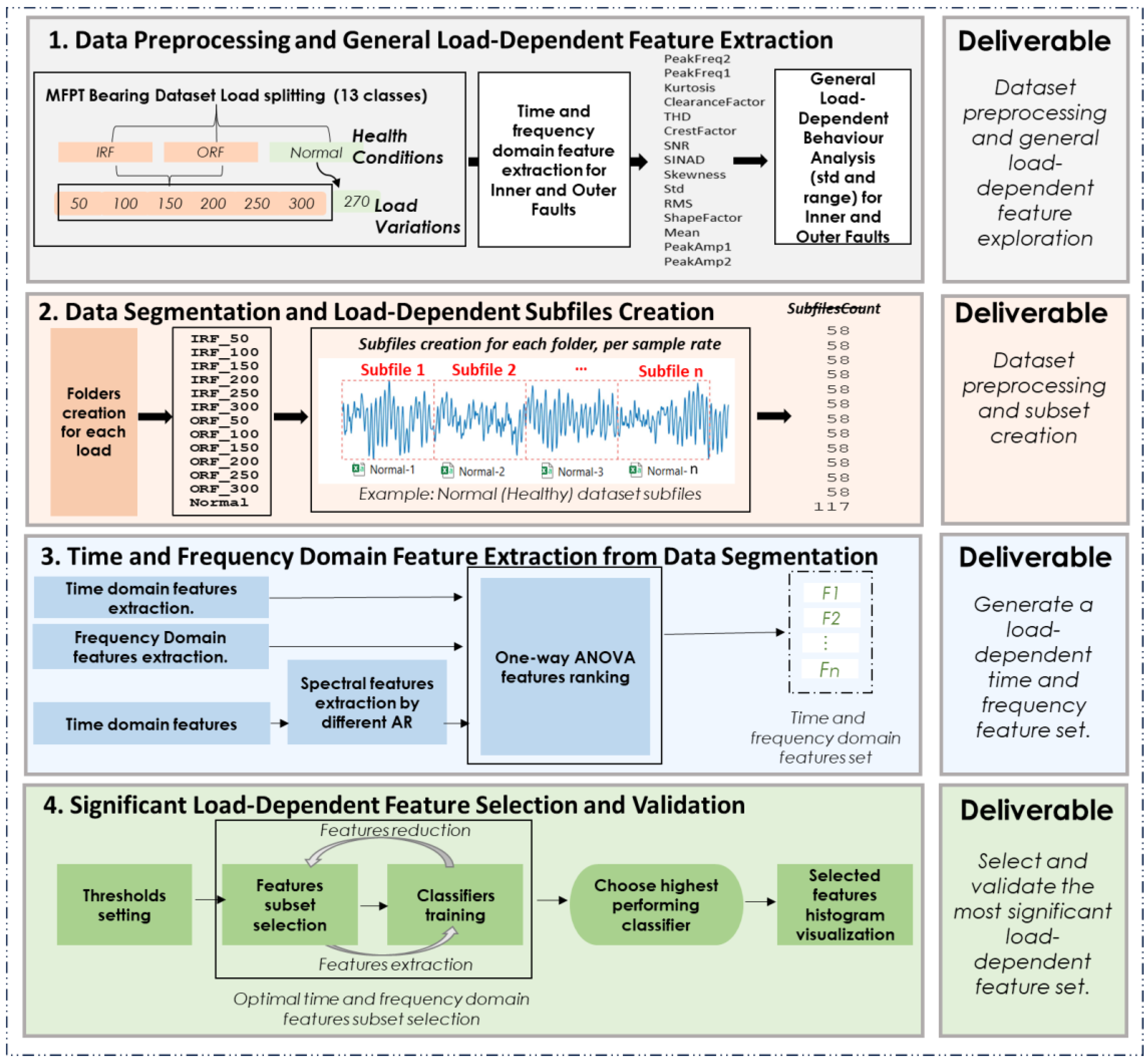
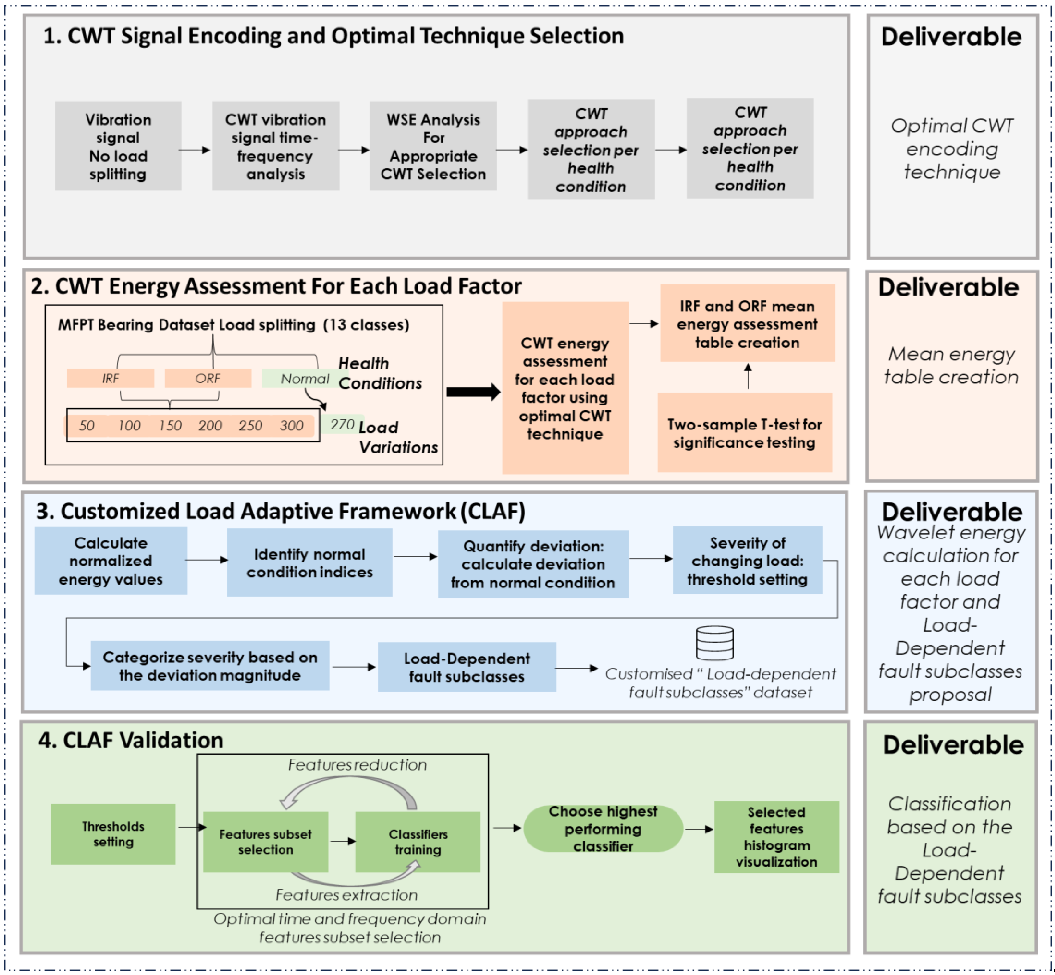
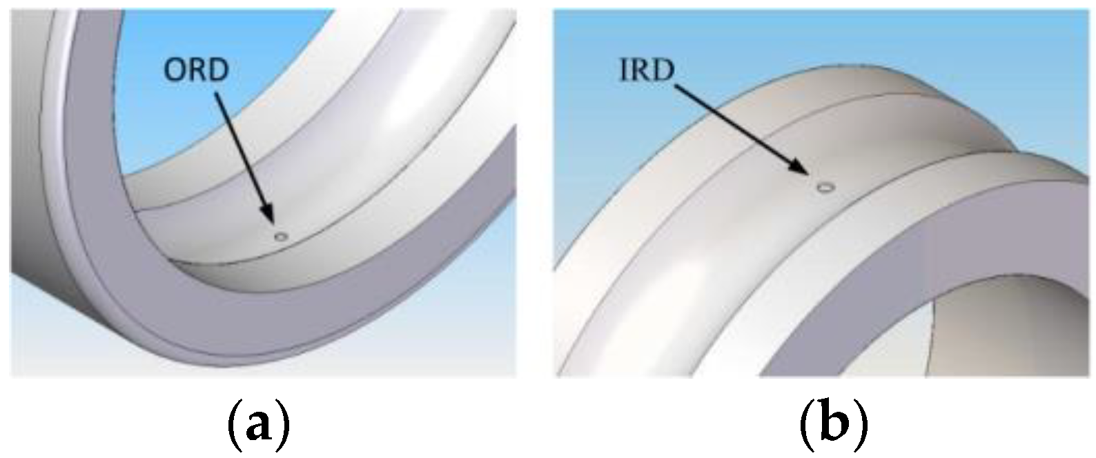
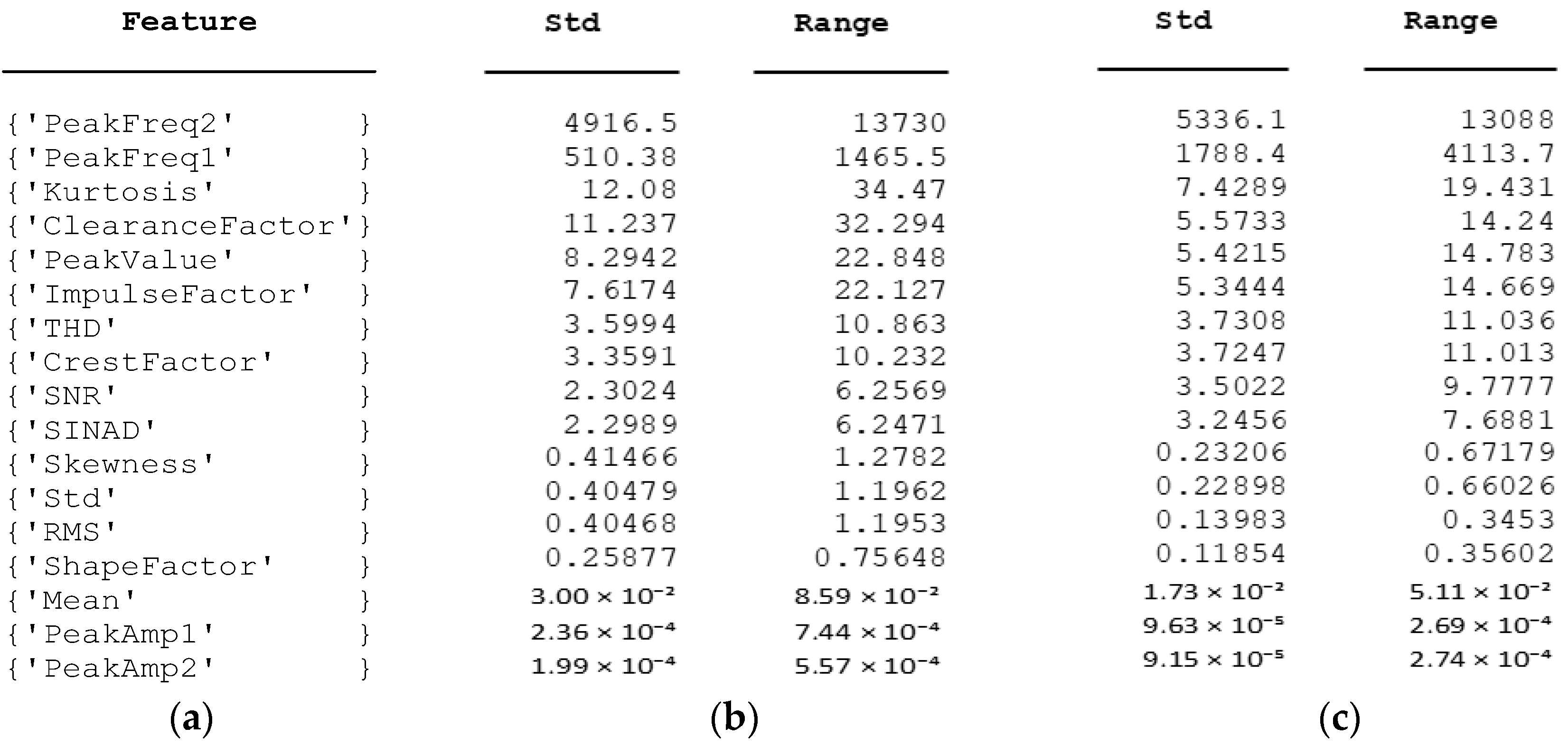
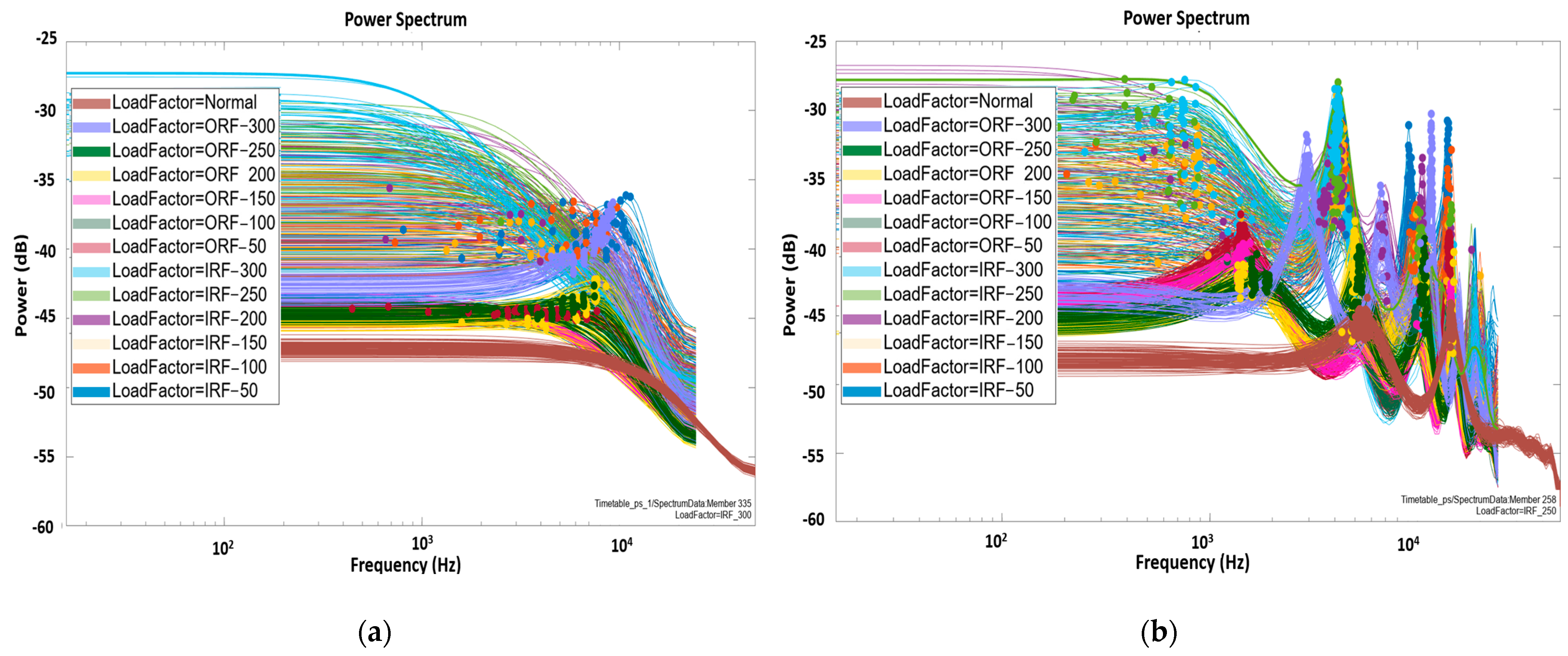
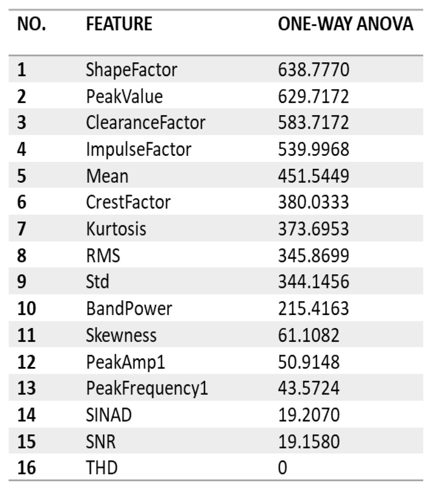
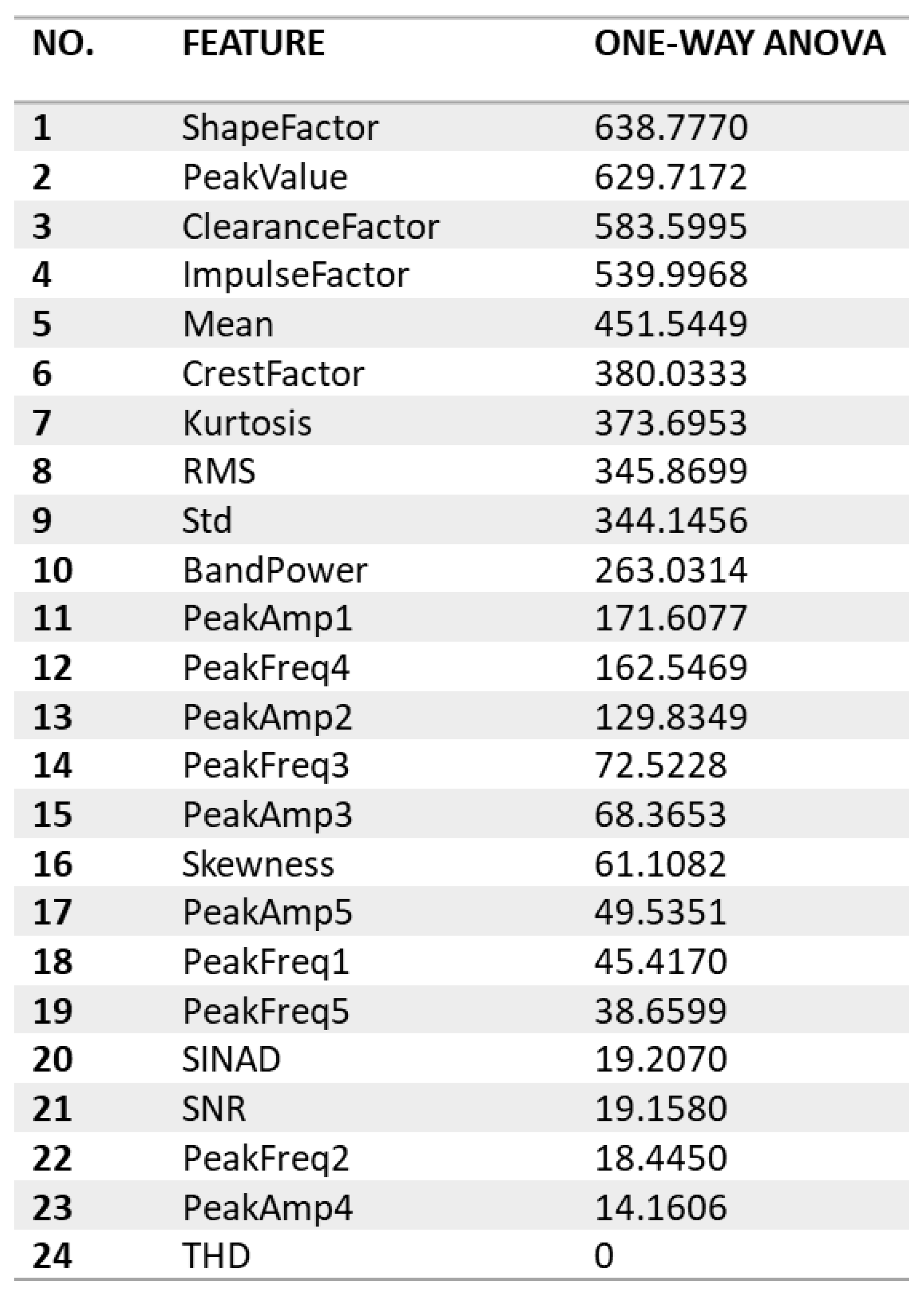
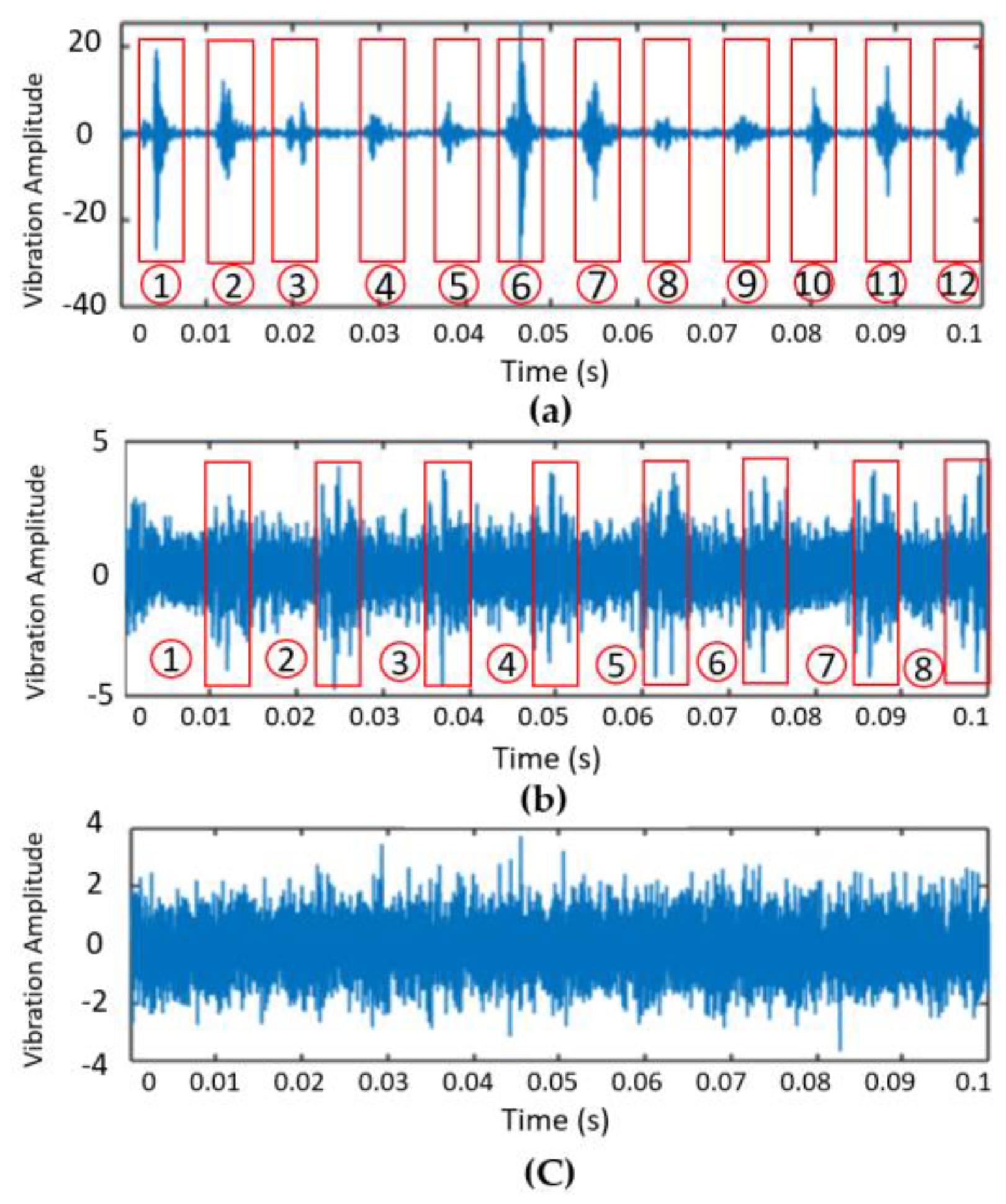
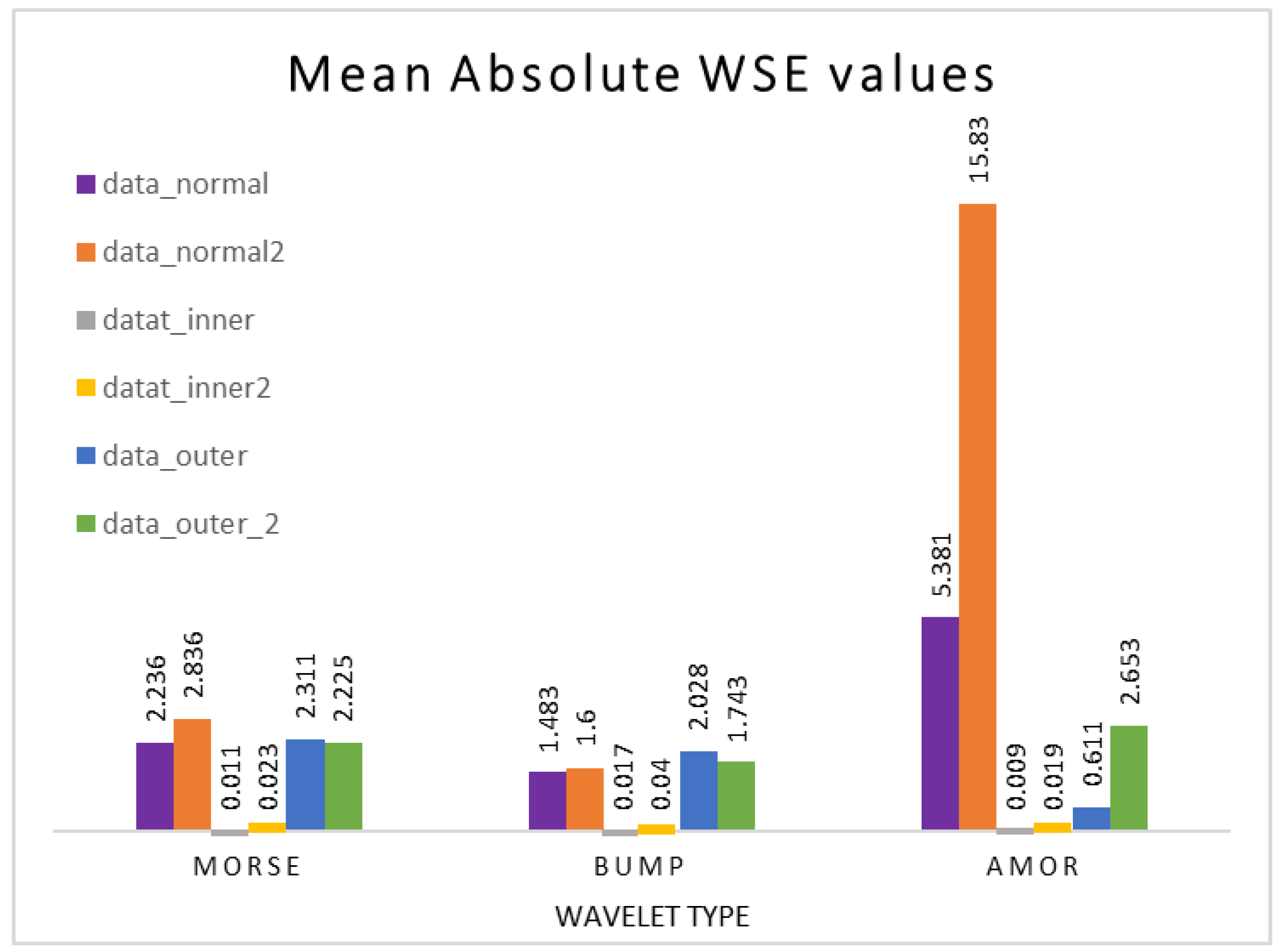
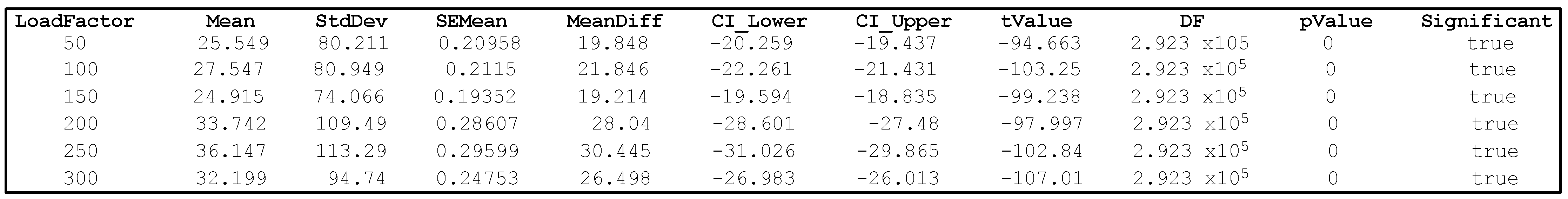
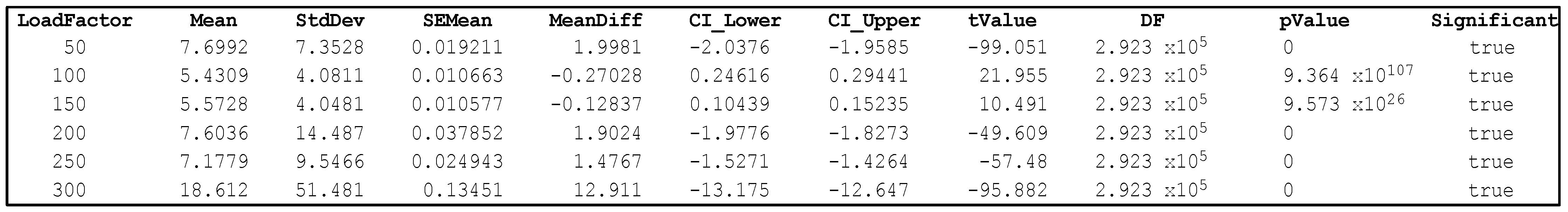
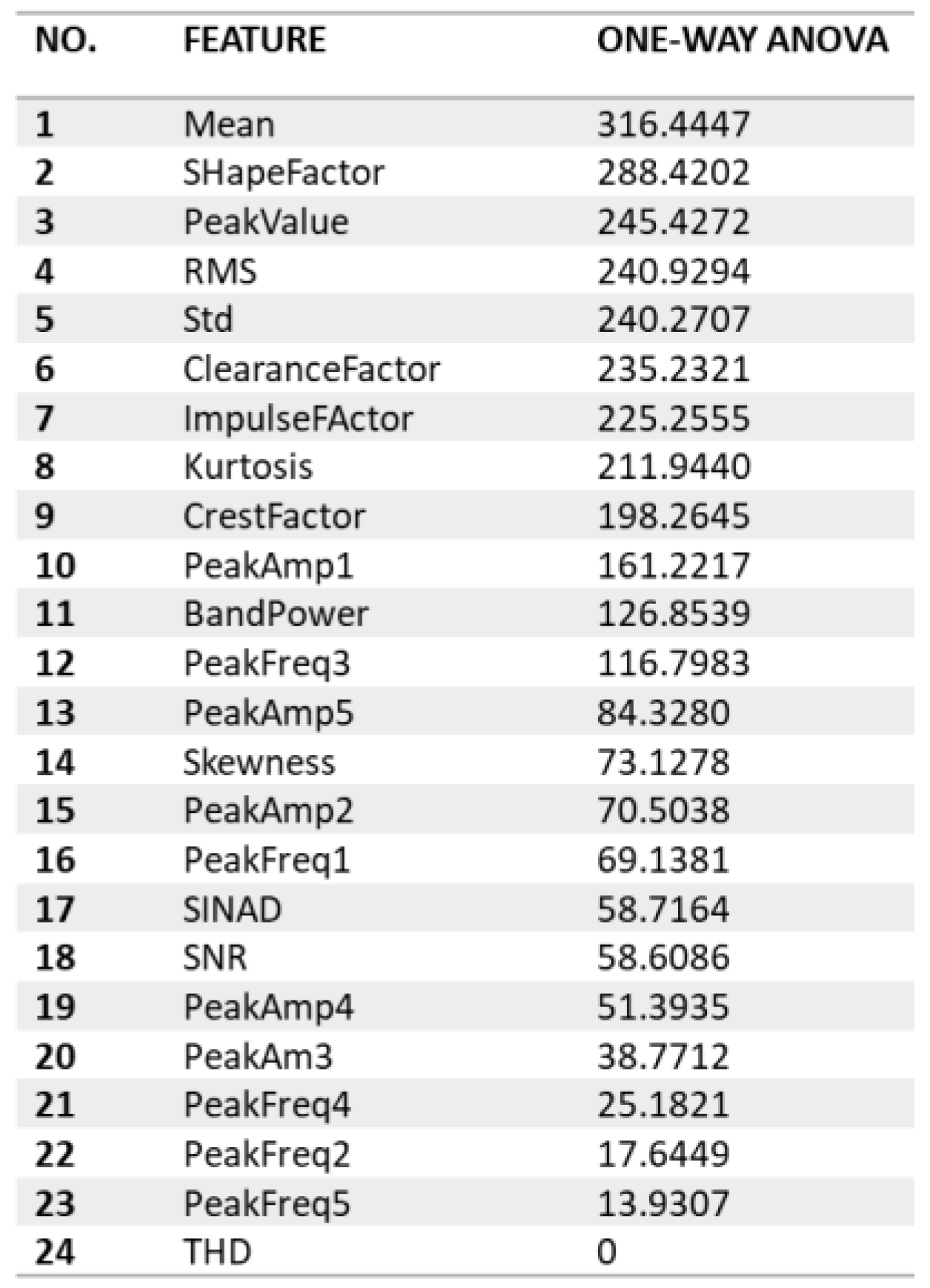
Table 1.
Traditional statistical features.
| Parameter | Formula | Description |
|---|---|---|
| Peak or Max | The highest amplitude value is observed within a given signal or dataset. | |
| Root Mean Square (RMS) | Gives a measure of the magnitude of the signal. | |
| Skewness | Measures the asymmetry of the distribution about the mean. | |
| Standard deviation (std) | The square root of the variance represents the average deviation from the mean. | |
| Kurtosis | Indicates the “tailedness” of the distribution. A high kurtosis might indicate the presence of outliers or impulses in the signal. | |
| Crest Factor | The ratio of the peak amplitude to its RMS value indicates the relative sharpness of peaks. | |
| Peak to Peak | Difference between the maximum and minimum values of the signal. | |
| Impulse Factor | Highlights the impulsive behaviours indicative of machinery faults. |
In the table, N is the sample size, represents individual data points and is the average data point.
Table 2.
Frequency domain features.
| Parameter | Formula | Description | |
|---|---|---|---|
| Harmonic Features | THD | Frequency domain, measuring the distortion caused by harmonics in the signal. | |
| SNR | Compares the level of a desired signal to the level of background noise. | ||
| SINAD | A measure of signal quality compares the level of desired signal to the level of background noise and harmonics. | ||
| Spectral Features | Peak amplitude | Represents the highest point (or peak) of the signal’s waveform when viewed in the frequency domain. | |
| Peak frequency | Corresponds to the frequency component that is most prominent or dominant in the signal. | ||
| Band power | Quantifies the total energy within a specific frequency range, providing insights into the distribution of signal energy across the spectrum. | ||
In the context of frequency domain analysis, is the amplitude of the fundamental frequency, and is the amplitude of the i-th harmonic. For SNR and SINAD calculations, is the signal power, is the noise power, and is the power of harmonic distortion. Peak amplitude is the frequency domain’s complex value at bin . is the complex value at frequency bin ‘f’, and represents its squared magnitude.
Table 3.
IRF dataset splitting per load.
| Inner Fault Dataset | Code | Load (lbs/kg) | Sampling Rate (Hz) | Duration (s) |
|---|---|---|---|---|
| baseline_2 | data_normal | 270/122.47 | 97,656 | 6 |
| InnerRaceFault_vload_2 | IRF_50 | 50/22.68 | 48,828 | 3 |
| InnerRaceFault_vload_3 | IRF_100 | 100/45.36 | 48,828 | 3 |
| InnerRaceFault_vload_4 | IRF_150 | 150/68.04 | 48,828 | 3 |
| InnerRaceFault_vload_5 | IRF_200 | 200/90.72 | 48,828 | 3 |
| InnerRaceFault_vload_6 | IRF_250 | 250/113.40 | 48,828 | 3 |
| InnerRaceFault_vload_7 | IRF_300 | 300/136.08 | 48,828 | 3 |
Table 4.
ORF dataset splitting per load.
| Outer Fault Dataset | Code | Load (lbs/kg) | Sampling Rate (Hz) | Duration (s) |
|---|---|---|---|---|
| baseline_2 | data_normal | 270/122.47 | 97,656 | 6 |
| OuterRaceFault_vload_2 | ORF_50 | 50/22.68 | 48,828 | 3 |
| OuterRaceFault_vload_3 | ORF_100 | 100/45.36 | 48,828 | 3 |
| OuterRaceFault_vload_4 | ORF_150 | 150/68.04 | 48,828 | 3 |
| OuterRaceFault_vload_5 | ORF_200 | 200/90.72 | 48,828 | 3 |
| OuterRaceFault_vload_6 | ORF_250 | 250/113.40 | 48,828 | 3 |
| OuterRaceFault_vload_7 | ORF_300 | 300/136.08 | 48,828 | 3 |
Table 5.
General time and frequency domain features (IRD).
| LoadFactor (lbs) | Clearance Factor | Crest Factor | Impulse Factor | Kurtosis | Mean | Peak Value | RMS | Shape Factor | Skewness | Std | SINAD * | SNR * | THD * |
|---|---|---|---|---|---|---|---|---|---|---|---|---|---|
| 50 | 40.04 | 15.462 | 28.69 | 27.97 | −0.22 | 27.50 | 1.78 | 1.86 | 0.62 | 1.76 | −21.32 | −21.307 | −5.36 |
| 100 | 37.30 | 14.488 | 26.96 | 30.53 | −0.22 | 26.59 | 1.84 | 1.86 | 0.87 | 1.82 | −21.05 | −21.027 | −0.53 |
| 150 | 33.30 | 13.249 | 24.31 | 33.13 | −0.22 | 23.06 | 1.74 | 1.84 | 1.28 | 1.72 | −19.05 | −19.046 | −10.06 |
| 200 | 38.15 | 13.537 | 26.92 | 37.28 | −0.21 | 27.38 | 2.02 | 1.99 | 1.15 | 2.01 | −18.22 | −18.208 | −6.31 |
| 250 | 37.52 | 13.022 | 26.18 | 37.49 | −0.20 | 27.14 | 2.08 | 2.01 | 0.72 | 2.08 | −17.70 | −17.684 | −5.46 |
| 300 | 35.24 | 12.998 | 25.17 | 35.30 | −0.19 | 25.58 | 1.97 | 1.94 | 0.68 | 1.96 | −17.35 | −17.341 | −8.41 |
| 270 ** | 7.75 | 5.230 | 6.56 | 3.02 | −0.14 | 4.65 | 0.89 | 1.25 | 0.00 | 0.88 | −23.60 | −23.598 | −11.39 |
* Frequency domain features. ** Normal health condition.
Table 6.
General time and frequency domain features (ORF).
| LoadFactor (lbs) | Clearance Factor | Crest Factor | Impulse Factor | Kurtosis | Mean | Peak Value | RMS | Shape Factor | Skewness | Std | SINAD * | SNR * | THD * |
|---|---|---|---|---|---|---|---|---|---|---|---|---|---|
| 50 | 10.26 | 6.39 | 8.48 | 5.09 | −0.19 | 6.35 | 0.99 | 1.33 | 0.04 | 0.98 | −14.41 | −14.40 | −11.97 |
| 100 | 9.15 | 5.84 | 7.62 | 4.40 | −0.18 | 4.93 | 0.84 | 1.31 | −0.01 | 0.82 | −13.15 | −13.12 | −9.06 |
| 150 | 9.54 | 6.10 | 7.94 | 4.04 | −0.18 | 5.21 | 0.85 | 1.30 | −0.04 | 0.83 | −12.59 | −12.56 | −9.934 |
| 200 | 21.81 | 12.46 | 17.67 | 11.90 | −0.17 | 12.28 | 0.99 | 1.42 | 0.31 | 0.97 | −17.54 | −17.52 | −5.54 |
| 250 | 15.03 | 9.07 | 12.30 | 6.59 | −0.16 | 8.66 | 0.96 | 1.36 | 0.12 | 0.94 | −16.09 | −16.06 | −4.92 |
| 300 | 27.18 | 12.92 | 20.80 | 17.69 | −0.16 | 19.43 | 1.50 | 1.61 | 0.27 | 1.50 | −15.10 | −15.10 | −14.69 |
| 270 ** | 7.75 | 5.23 | 6.56 | 3.02 | −0.14 | 4.65 | 0.89 | 1.25 | 0.01 | 0.88 | −23.60 | −23.60 | −11.39 |
* Frequency domain features. ** Normal health condition.
Table 7.
Spectral features by AR model (IRF and ORF).
| LoadFactor | PeakAmp1 | PeakAmp2 | PeakFreq1 | PeakFreq2 | BandPower | |||||
|---|---|---|---|---|---|---|---|---|---|---|
| Inner | Outer | Inner | Outer | Inner | Outer | Inner | Outer | Inner | Outer | |
| 50 | 0.00034 | 0.000109 | 0.00031 | 0.000093 | 4363.937 | 1413.267 | 13,991.090 | 14,179.042 | 1.474 | 0.454 |
| 100 | 0.00046 | 0.000075 | 0.00012 | 0.000028 | 4256.059 | 1379.739 | 13,968.668 | 14,258.280 | 1.476 | 0.322 |
| 150 | 0.00046 | 0.000080 | 0.00005 | 0.000036 | 4191.394 | 1377.111 | 14,127.206 | 14,462.995 | 1.330 | 0.327 |
| 200 | 0.00031 | 0.000063 | 0.00011 | 0.000058 | 4025.383 | 4947.698 | 10,622.786 | 1391.188 | 1.663 | 0.461 |
| 250 | 0.00061 | 0.000058 | 0.00009 | 0.000049 | 4124.988 | 1621.552 | 10,365.553 | 5212.034 | 1.807 | 0.430 |
| 300 | 0.00077 | 0.000302 | 0.00058 | 0.000296 | 4081.332 | 2915.517 | 748.668 | 11,675.566 | 1.618 | 1.101 |
| Normal 270 | 0.00003 | 0.000028 | 0.00003 | 0.000028 | 5490.855 | 5490.855 | 14,478.764 | 14,478.764 | 0.279 | 0.302 |
Table 8.
Dataset segmentation and subfiles creation demonstration.
| Dataset Segmentation | CSV Files | Code | Load Factor | Subfiles Count |
|---|---|---|---|---|
Example on baseline (Normal) with Matlab code. The segment is based on ratio, i.e., each segment in inner and outer fault contains 2500 samples, and each sample in Normal condition contains 5000 data points.   |  | IRF_50 | {‘IRF−50’} | 58 |
| IRF_100 | {‘IRF−100’} | 58 | ||
| IRF_150 | {‘IRF−150’} | 58 | ||
| IRF_200 | {‘IRF−200’} | 58 | ||
| IRF_250 | {‘IRF−250’} | 58 | ||
| IRF_300 | {‘IRF−300’} | 58 | ||
| ORF_50 | {‘ORF−50’ } | 58 | ||
| ORF_100 | {‘ORF−100’ } | 58 | ||
| ORF_150 | {‘ORF−150’} | 58 | ||
| ORF_200 | {‘ORF−200’} | 58 | ||
| ORF_250 | {‘ORF−250’} | 58 | ||
| ORF_300 | {‘ORF−300’} | 58 | ||
| Normal | {‘Normal’} | 117 |
Table 9.
Classifier performance across feature selection thresholds for AR model (a) and peak = 1.
| No. of Features Used in Classifier Training | Classifier Name | Accuracy Score on the Testing Dataset |
|---|---|---|
| Top 13 >20 | Boosted Trees | 74.1% |
| Top 8 >345 | Narrow Neural Network | 72.8% |
| Top 7 >373 | Bilayered Neural Network | 73.5% |
| Top 2 >629 | Fine Gaussian SVM | 59.9% |
Table 10.
Classifier performance across feature selection thresholds for AR model (b) order fifteen, peak = 5.
Table 10.
Classifier performance across feature selection thresholds for AR model (b) order fifteen, peak = 5.
| Number of Selected Features from ANOVA Ranking | Classifier | Accuracy Score on the Testing Dataset |
|---|---|---|
| Top 19 >20 | Bagged trees | 86.4% |
| Top 14 >72 | Cubic SVM | 86.4% |
| Top 13 >129 | Quadratic SVM | 83.3% |
| Top 11 >171 | Quadratic Discriminant | 84.6% |
| Top 8 >345 | Quadratic SVM | 76.5% |
Table 11.
Top 14 selected features distinguishing load-dependent fault types: a histogram visualization.
Table 11.
Top 14 selected features distinguishing load-dependent fault types: a histogram visualization.
| Load Factor Color Code Legend for the Top 14 Features Ranked by One-Way ANOVA | |||
|---|---|---|---|
 | |||
| Features (ANOVA Rank) | Features Histogram | Features (ANOVA Rank) | Features Histogram |
| 1. Shape Factor |  | 2. Peak Value |  |
| 3. ClearanceFactor |  | 4. ImpulseFactor |  |
| Mean |  | 6. CrestFactor |  |
| 7. Kurtosis |  | 8. RMS |  |
| 9. Standard deviation |  | 10. Band Power |  |
| 11. Peak Amplitude1 |  | 12. Peak Frequency4 |  |
| 13. Peak Amplitude 2 |  | 14. PeakFrequency3 |  |
Table 12.
Comparative Visualisation of Health Condition Signals: 2D Time–Frequency Diagrams Using Three Types of Mother Wavelet Functions.
Table 12.
Comparative Visualisation of Health Condition Signals: 2D Time–Frequency Diagrams Using Three Types of Mother Wavelet Functions.
| Health State | Inner | Outter | Normal |
|---|---|---|---|
| Dataset | InnerRaceFault_vload_1 | ‘OuterRaceFault_3.mat’ | ‘baseline_1.mat’ |
| 2D time-frequency diagrams | |||
| Bump |  | ||
| Morse |  | ||
| Amor |  | ||
The color bar adjacent to the scalogram represents the magnitude of the wavelet coefficients. Colors closer to red indicate higher values, which may correspond to signal peaks or areas of high power, while colors closer to blue represent lower values.
Table 13.
WSE scores comparison with three types mother of wavelet functions.
| Health State | Training Set | Code | Morse | Bump | Amor |
|---|---|---|---|---|---|
| Normal | baseline_1 | data_normal | 2.236 | 1.483 | 5.381 |
| baseline_2 | data_normal2 | 2.836 | 1.600 | 15.830 | |
| WSE Avg. for 0.1 s | 2.536 | 1.541 | 10.603 | ||
| Inner | InnerRaceFault_vload_1 | datat_inner | 0.011 | 0.017 | 0.009 |
| InnerRaceFault_vload_2 | datat_inner2 | 0.023 | 0.040 | 0.019 | |
| WSE Avg. for 0.1 s | 0.017 | 0.028 | 0.014 | ||
| Outer | OuterRaceFault_3 | data_outer | 2.311 | 2.028 | 0.611 |
| OuterRaceFault_1 | data_outer_2 | 2.225 | 1.743 | 2.653 | |
| WSE Avg. for 0.1 s | 2.268 | 1.886 | 1.632 | ||
Table 14.
IRF and ORF CWT mean energy.
| Inner Race Fault Type | Outer Race Fault Type | |||
|---|---|---|---|---|
| Load Factor (lbs) | MeanEnergy | Mean Energy Increase % | MeanEnergy | Mean Energy Increase % |
| 50 | 25.549 | 347.70% | 7.699 | 35.16% |
| 100 | 27.547 | 383.65% | 5.431 | 4.76% |
| 150 | 24.915 | 337.68% | 5.573 | 2.08% |
| 200 | 33.742 | 491.88% | 7.604 | 33.35% |
| 250 | 36.147 | 533.49% | 7.178 | 25.90% |
| 270 | 5.7012 | 0% (baseline) | 5.701 | 0% (baseline) |
| 300 | 32.199 | 464.25% | 18.612 | 226.88% |
Table 15.
IRF and ORF load-dependent subclasses through CLAF.
| LoadFactor (lb) | Mean Energy | NormalizedEnergy | Deviation | Load-Dependent Subclasses | ||||
|---|---|---|---|---|---|---|---|---|
| Fault Type | Inner | Outer | Inner | Outer | Inner | Outer | Inner | Outer |
| 50 | 25.549 | 7.6992 | 0.14035 | 0.05758 | 0.1403 | 0.05758 | {‘Mild’} | {‘Mild’} |
| 100 | 27.547 | 5.4309 | 0.15053 | 0.023062 | 0.15053 | 0.023062 | {‘Mild’} | {‘Mild’} |
| 150 | 24.915 | 5.5728 | 0.14063 | 0.031372 | 0.14063 | 0.031372 | {‘Mild’} | {‘Mild’} |
| 200 | 33.742 | 7.6036 | 0.28444 | 0.092816 | 0.28444 | 0.092816 | {‘Moderate’} | {‘Mild’} |
| 250 | 36.147 | 7.1779 | 0.29911 | 0.061822 | 0.29911 | 0.061822 | {‘Moderate’} | {‘Mild’} |
| 270 | 5.7012 | 5.7012 | 0.00930 | 0.027659 | 0 | 0 | {‘Normal’} | {‘Normal’} |
| 300 | 32.199 | 18.612 | 0.23412 | 0.89814 | 0.23412 | 0.89814 | {‘Moderate’} | {‘Severe’} |
Table 16.
CLAF load-dependent subclasses classifiers training on various feature subsets.
| Classifier | ANOVA Ranking | TTime 1 | Validation Dataset | Testing Dataset | ||||
|---|---|---|---|---|---|---|---|---|
| (s) | VA 2 | NA 3 | MA 4 | MoA 5 | SA 6 | Overall Accuracy | ||
| RUSBoostedTrees | Top 20 >26 | 11.539 | 92.6% | 100% | 92.4% | 91.2% | 100% | 93.8% |
| Fine Tree | Top 17 >58.6 | 4.393 | 92.6% | 100% | 95.7% | 82.4% | 100% | 93.8% |
| Wide neural network | Top 10 >161 | 18.155 | 91.2% | 100% | 97.8% | 88.2% | 100% | 96.3% |
| Cubic SVM | Top7 (a) >215 | 8.1055 | 93.1% | 100% | 96.7% | 82.4% | 100% | 94.4% |
| Medium Gaussian SVM | Top 7 (b) | 5.8059 | 91.6% | 100% | 96.7% | 82.4% | 100% | 94.4% |
| Fine Gaussian SVM | Top 5 >240 | 12.711 | 92.9% | 100% | 97.8% | 82.4% | 100% | 95.1% |
1 TTime is the training time, 2 VA is the validation accuracy, 3 NA is the normal (fault-free) condition accuracy, 4 MA is the mild state accuracy, 5 MoA is the moderate state accuracy, and 6 SA is the severe state accuracy.
Disclaimer/Publisher’s Note: The statements, opinions and data contained in all publications are solely those of the individual author(s) and contributor(s) and not of MDPI and/or the editor(s). MDPI and/or the editor(s) disclaim responsibility for any injury to people or property resulting from any ideas, methods, instructions or products referred to in the content. |
© 2024 by the authors. Licensee MDPI, Basel, Switzerland. This article is an open access article distributed under the terms and conditions of the Creative Commons Attribution (CC BY) license (https://creativecommons.org/licenses/by/4.0/).
Share and Cite
MDPI and ACS Style
Hejazi, S.Z.; Packianather, M.; Liu, Y. A Novel Customised Load Adaptive Framework for Induction Motor Fault Classification Utilising MFPT Bearing Dataset. Machines 2024, 12, 44. https://doi.org/10.3390/machines12010044
AMA Style
Hejazi SZ, Packianather M, Liu Y. A Novel Customised Load Adaptive Framework for Induction Motor Fault Classification Utilising MFPT Bearing Dataset. Machines. 2024; 12(1):44. https://doi.org/10.3390/machines12010044
Chicago/Turabian StyleHejazi, Shahd Ziad, Michael Packianather, and Ying Liu. 2024. "A Novel Customised Load Adaptive Framework for Induction Motor Fault Classification Utilising MFPT Bearing Dataset" Machines 12, no. 1: 44. https://doi.org/10.3390/machines12010044
Note that from the first issue of 2016, this journal uses article numbers instead of page numbers. See further details here.