Future Runoff Variation and Flood Disaster Prediction of the Yellow River Basin Based on CA-Markov and SWAT

Abstract

The purpose of this paper is to simulate the future runoff change of the Yellow River Basin under the combined effect of land use and climate change based on Cellular automata (CA)-Markov and Soil & Water Assessment Tool (SWAT). The changes in the average runoff, high extreme runoff and intra-annual runoff distribution in the middle of the 21st century are analyzed. The following conclusions are obtained: (1) Compared with the base period (1970–1990), the average runoff of Tangnaihai, Toudaoguai, Sanmenxia and Lijin hydrological stations in the future period (2040–2060) all shows an increasing trend, and the probability of flood disaster also tends to increase; (2) Land use/cover change (LUCC) under the status quo continuation scenario will increase the possibility of future flood disasters; (3) The spring runoff proportion of the four hydrological stations in the future period shows a decreasing trend, which increases the risk of drought in spring. The winter runoff proportion tends to increase; (4) The monthly runoff proportion of the four hydrological stations in the future period tends to decrease in April, May, June, July and October. The monthly runoff proportion tends to increase in January, February, August, September and December.

1. Introduction

The Chinese government promoted the “ecological protection and high quality development of the Yellow River Basin” as a national development strategy in 2019, and pointed out that there are some problems to be solved in the basin, such as water shortage. With its rapid increase in population and the rapid expansion of the economy, water shortage is becoming more and more serious [1], which restricts its high quality and rapid development. Runoff is an important part of water resources in the Yellow River Basin. Therefore, the analysis and simulation of runoff change is very important for the management and effective utilization of water resources in the Yellow River Basin.

Many scholars have simulated future runoff variation in different rivers, such as the Yellow River [2,3,4], Hoeya River [5], Altmühl River [6], Beijiang River [7], and the upper reaches of the Grande River [8]. For example, Li et al. [9] simulated the future runoff variation in the upper reaches of the Yellow River under two climate scenarios (A2 and B2) using seven CMIP3 models. The results showed that the runoff will tend to decrease in the future, and the probability and severity of flood and drought disasters will all increase. Li et al. [10] simulated the runoff variation in the source region of the Yellow River from 2010 to 2020 under two climate scenarios (A2 and B2), and showed that the runoff will decrease gradually in the future. Wei et al. [11] imported the climatic data from the BCC-CSM1.1 model into the Variable Infiltration Capacity (VIC) hydrological model and estimated the runoff change in the upper reaches of the Yellow River from 2011 to 2050. The results indicated that, compared with the runoff from 1971 to 2010, the runoff in this area increases by 2.65%, 2.66% and 8.07%, respectively, under the three representative concentration path (RCP) scenarios (RCP2.6, RCP4.5 and RCP8.5). Lu et al. [12] used RegCM4 to predict the runoff changes in the source area of the Yellow River from 2041 to 2060 under three RCP scenarios (RCP2.6, RCP4.5 and RCP8.5). The results showed that the runoff increases by more than 3%. There are some inconsistent results in the existing studies, which may be caused by the use of different global climate model data.

In fact, the runoff change is the result of the joint action of many factors. In addition to climate factors, soil type, topographical features and land use/cover change (LUCC), which are also the input to the Soil & Water Assessment Tool (SWAT) model, are also key factors affecting the change in runoff; however, the soil type and topographical features do not change in a short time [13,14,15]. LUCC affects the hydrological cycle process by changing transpiration and surface confluence [16,17,18], and then affects its runoff and its intra-annual runoff distribution. However, previous studies have only considered the impact of climate change on the future runoff of the Yellow River basin, but did not take into account the impact of LUCC on the future runoff, which may be due to the lack of high-resolution land use data.

The purpose of this paper is to simulate the future runoff change in the Yellow River Basin under the combined effect of land use and climate change. Firstly, the cellular automata (CA)-Markov model was applied to simulate the land use data of the Yellow River Basin in 2050 under the status quo continuation scenario. Then, the SWAT model was applied to simulate the runoff from 2040 to 2060 under the combined action of land use and climate change. Finally, the difference between average runoff, seasonal runoff proportion, monthly runoff proportion and high extreme runoff in the future period (2040–2060) and base period (1970–1990) was analyzed.

2. Study Area, Data and Methods

2.1. Study Area

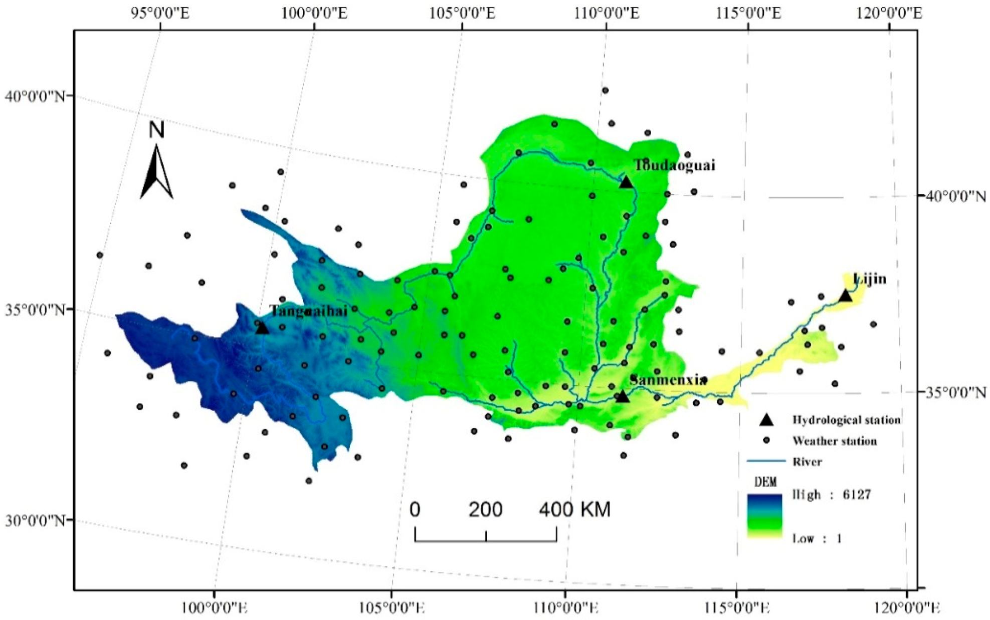
The Yellow River basin lies around 95°53′~119°05′ E, 32°10′~41°50′ N (Figure 1), it originates from the Bayankala mountains, and flows into the Bohai sea. The Yellow River spans 5464 km and covers 79.5 × 10⁴ km² (including the inner river area), accounting for 8% of China. Most of the regions belong to arid and semi-arid regions. Its precipitation decreases from southeast to northwest, with an average of 476mm. The overall distribution of temperature is gradually decreased from south to north and from east to west, with an annual average temperature between −4 and 14 °C. Its evaporation is different and increases from southeast to northwest. The water resources in the basin are deficient and the ecological environment is fragile under the influence of climate change and human activities. In addition, the basin is also one of the most important bases for the production of grain and agricultural products in China, accounting for about 13.4% of China’s total amount of agricultural products. The total area of cultivated land in the basin is 20.2346 million hm², accounting for about 16.6% [19]. The shortage of water resources in the basin poses a great threat to China’s food security.

2.2. Data Sources

(1) The monthly runoff data of the Tangnaihai, Toudaoguai, Sanmenxia and Lijin stations from 1967 to 1990 are obtained from the Yellow River Water Conservancy Commission (http://yrcc.gov.cn/, accessed on 1 January 2021). Tangnaihai hydrological station is a runoff monitoring station in the source area of the Yellow River. Toudaoguai hydrological station is the dividing point between the upper and middle reaches of the Yellow River. Sanmenxia hydrological station is an important national hydrological station, which is responsible for the flood control monitoring of the lower Yellow River. Lijin hydrological station is the last hydrological station in the Yellow River Basin.

(2) The Digital Elevation Model (DEM) data are downloaded from the Resource and Environmental Science Data Center of the Chinese Academy of Sciences (http://www.resdc.cn/, accessed on 1 January 2021), with a resolution of 1 km × 1 km.

(3) The land use data are downloaded from the Resource and Environmental Science Data Center of the Chinese Academy of Sciences (http://www.resdc.cn/, accessed on 1 January 2021), including 1980, 1995, 2005 and 2015, with a resolution of 1 km × 1 km.

(4) The soil data are derived from the World Soil Database with a resolution of 1 km × 1 km (http://westdc.westgis.ac.cn/, accessed on 1 January 2021).

(5) The 134 meteorological station data in and around the Yellow River are obtained from the China Meteorological Administration (http://www.cma.gov.cn, accessed on 1 January 2021).

(6) The climate data in the future period are derived from the five global climate models (https://esgf-node.llnl.gov/search/cmip5/, accessed on 1 January 2021), including MIROC-ESM-CHEM, NorES1-M, IPSL-CM5A-LR, GFDL-ESM2M, and HadGEM2-ES (

Table 1. The basic information of the five global climate models.

Global Climate Model	Country	Resolution (Longitude × Latitude)
GFDL-ESM2M	America	2° × 2.5°
HadGEM2-ES	England	1.25° × 1.875°
IPSL-CM5A-LR	France	1.875° × 3.75°
MIROC-ESM-CHEM	Japan	2.8° × 2.8°
NorESM1-M	Norway	1.875° × 2.5°

). These five models are widely used to assess China’s future climate change [20,21]. Each global climate model includes daily mean temperature data, daily maximum temperature data, daily minimum temperature data and daily precipitation data under four RCP scenarios. RCP2.6, RCP4.5, RCP6.0 and RCP8.5 scenarios indicate that the earth’s radiation forcing levels in 2100 are 2.6 w/m², 4.5 w/m², 6.0 w/m² and 8.5 w/m², respectively.

2.3. Methods

2.3.1. Delta Method

The spatial resolution of global climate model data is very low, so it is difficult to accurately and effectively show the climate change on the watershed scale. Therefore, it is necessary to use a downscaling method to improve its accuracy when studying the watershed scale.

The Delta method can correct the data bias of multiple weather stations at the same time, and its operation process is relatively simple, which has been widely used by scholars [22,23,24]. Therefore, based on the observation data of 134 meteorological stations in and around the Yellow River Basin from 1985 to 2005, the Delta method is used to process the precipitation, maximum temperature and minimum temperature data of five CMIP5 models from 2040 to 2060, including MIROC-ESM-CHEM, NorES1-M, IPSL-CM5A-LR, GFDL-ESM2M and HadGEM2-ES, respectively. The specific calculation formula is as follows:

$$P_{Fut}=P_{His}\times \frac{[P_{Gfut}]{}_{Mon}}{[P_{Ghis}]{}_{Mon}}$$

(1)

$${Tmax}_{Fut}={Tmax}_{His}+\left\{[Tmax{}_{Gfut}]{}_{Mon}-[Tmax{}_{Ghis}]{}_{Mon}\right\}$$

(2)

$${Tmin}_{Fut}={Tmin}_{His}+\left\{[Tmin{}_{Gfut}]{}_{Mon}-[Tmin{}_{Ghis}]{}_{Mon}\right\}$$

(3)

In the formula, $P_{Fut}$, ${Tmax}_{Fut}$, ${Tmin}_{Fut}$ represent the future precipitation, maximum temperature and minimum temperature data of each meteorological station after downscaling, respectively; $P_{His}$, ${Tmax}_{His}$, ${Tmin}_{His}$ represent the precipitation, maximum temperature and minimum temperature observed data at each meteorological station in the historical period, respectively; $[P_{Gfut}]{}_{Mon}$, $[Tmax{}_{Gfut}]{}_{Mon}$, $[Tmin{}_{Gfut}]{}_{Mon}$ represent the monthly scale precipitation, maximum temperature and minimum temperature data of the CMIP5 model in the future period, respectively; $[P_{Ghis}]{}_{Mon}$, $[Tmax{}_{Ghis}]{}_{Mon}$, $[Tmin{}_{Ghis}]{}_{Mon}$ represent the monthly precipitation, maximum temperature and minimum temperature data of the CMIP5 model in the historical period, respectively.

2.3.2. CA-Markov Model

The CA-Markov model effectively combines the advantages of the CA model and Markov model, greatly improves the accuracy of future land use simulation results, and has been widely used [25,26]. Therefore, the CA-Markov model is chosen as the method to simulate the land use of the Yellow River Basin in 2050 in this paper.

The CA model can be expressed by the following formula:

S_t+1 = f(S_t,N)

(4)

where S represents a set of all cells, t and t + 1 represent different times, f represents a functional transformation between cells, and N represents the neighborhood of cells.

By analyzing the transition probability of random events from the initial period to another period, the Markov model can predict the situation in the future period on the basis of the initial period. It can be expressed in the following formula:

S_t+1 = P_ijS_t

(5)

where S_t and S_t+1 represent the land type matrix at time t and t + 1, respectively; P_ij represents the transfer probability matrix.

2.3.3. Kappa Coefficient

The Kappa coefficient is often used to verify the accuracy of the predicted land use map. It is generally believed that the accuracy of the prediction result is better if the Kappa value is greater than 0.75 [26,27].

Assuming that the total number of pixels is N, S is the number of correctly simulated grids. The real number of each class is a₁, a₂,…, a_c, respectively, while the simulated number of each class is b₁, b₂,…, b_c, respectively, the kappa coefficient (K) can be expressed in the following formulas:

$$K=\frac{P{}_0-P{}_c}{1-P{}_c}$$

(6)

$$P{}_0=\frac{S}{N}$$

(7)

$$P_c=\frac{a{}_1\times b{}_1+a{}_2\times b{}_2+\dots +a{}_c\times b{}_c}{N\times N}$$

(8)

2.3.4. SWAT Model

The SWAT model is a distributed hydrological model, and several studies showed that the SWAT model can be better applied to simulate not only streamflow and runoff but also nutrient loadings, water quality, pollution, etc., all over the world in different climate regions [28,29,30,31,32,33,34,35].

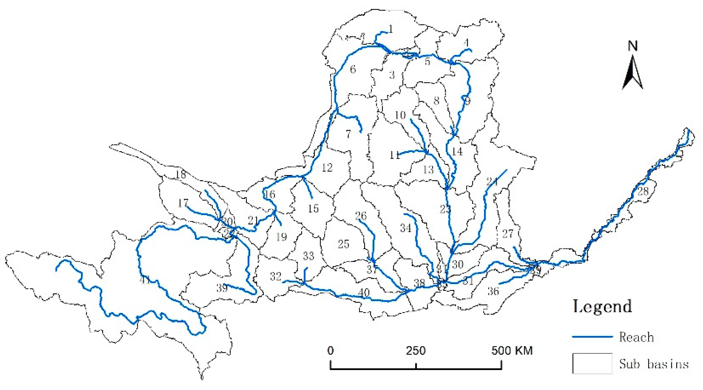
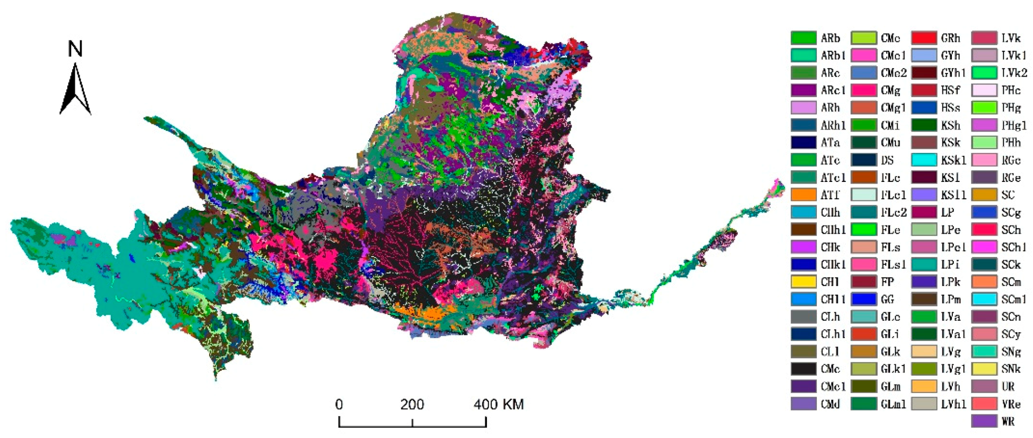
In this paper, firstly, the Yellow River Basin is divided into 33 sub basins according to the DEM data (Figure 2), and then, the Hydrological Response Units (HRUs) in each sub basin are divided according to the land use, slope and soil type data imported into the SWAT model. Slope data are calculated based on DEM data. The basic information of soil type data is displayed in Figure 3 and

Table 2. Names and abbreviations of soil types.

Name	Abbreviation	Name	Abbreviation	Name	Abbreviation
Cambic Arenosols	ARb	Salic Fluviosls	FLs	Gleyic Luvisols	LVg
Calcaric Arenosols	ARc	Fishpond	FP	Haplic Luvisols	LVh
Haplic Arenosols	ARh	Glaciers	GG	Calcic Luvisols	LVk
Aric Anthrosols	ATa	Eutric Gleysols	GLe	Calcaric Phaeozems	PHc
Cumulic Anthrosols	ATc	Gelic Gleysols	GLi	Gleyic Phaeozems	PHg
Fimic Anthrosols	ATf	Calcic Gleysols	GLk	Haplic Phaeozems	PHh
Haplic Chernozems	CHh	Mollic Gleysols	GLm	Calcaric Regosols	RGc
Calcic Chernozems	CHk	Haplic Greyzems	GRh	Eutric Regosols	RGe
Luvic Chernozems	CHl	Haplic Gypsisols	GYh	SOLONCHAKS	SC
Haplic Calcisols	CLh	Fibric Histosols	HSf	Gleyic Solonchaks	SCg
Luvic Calcisols	CLl	Terric Histosols	HSs	Haplic Solonchaks	SCh
Calcaric Cambisols	CMc	Haplic Kastanozems	KSh	Calcic Solonchaks	SCk
Dystric Cambisols	CMd	Calcic Kastanozems	KSk	Mollic Solonchaks	SCm
Eutric Cambisols	CMe	Luvic Kastanozems	KSl	Sodic Solonchaks	SCn
Gleyic Cambisols	CMg	LEPTOSOLS	LP	Gypsic Solonchaks	SCy
Gelic Cambisols	CMi	Eutric Leptosols	LPe	Gleyic Solonetz	SNg
Humic Cambisols	CMu	Gelic Leptosols	LPi	Calcic Solonetz	SNk
Dunes and shift sands	DS	Rendzic Leptosols	LPk	Urban, mining, etc.	UR
Calcaric Fluvisols	FLc	Mollic Leptosols	LPm	Eutric Vertisols	VRe
Eutric Fluvisols	FLe	Albic Luvsiols	LVa	Water bodies	WR

. The number of HRUs can affect the speed of SWAT model operation. Therefore, in order to take into account the accuracy and speed of SWAT model operation, it is not suitable to generate too many HRUs. The threshold values of land use, soil and slope are set to 15%, 15% and 15%, which means that land use, soil and slope below 15%, 15% and 15% will be merged into other types. Finally, 138 HRUs are generated.

Then, the soil attribute database and meteorological attribute database are established, respectively, according to the soil data and meteorological data. Finally, the SWAT model of the Yellow River Basin is established. Among them, 1967–1969 is the warm-up period, 1970–1980 is the calibration period, and 1981–1990 is the validation period. Its time step is months.

2.3.5. SWAT-CUP Software

SWAT-CUP is a software developed by the Swiss Federal Institute of Aquatic Science and Technology for calibrating the SWAT model. In SWAT-CUP software, there are 5 algorithms that can be selected to verify the parameters, namely SUFI2 algorithm, GLUE algorithm, ParaSOl algorithm, MCMC algorithm and PSO algorithm. The SUFI2 algorithm has the fastest operation process and high accuracy [36]. Therefore, the SUFI2 algorithm was selected to describe the uncertainty of the parameters based on a uniform distribution assumption. This algorithm is able to perform the approximation at a 95 percent prediction uncertainty level called 95PPU [37]. SUFI2 initially assumes large uncertainty in the parameters covering all the observed data at 95PPU level. This uncertainty is reduced in subsequent rounds until the difference between the upper and the lower parts of 95PPU—97.5% and 2.5% levels—is minimized and 95PPU includes 80–100% of the observations [38]. The SUFI2 algorithm uses a Latin hypercube sampling approach [39] where n parameters are combined in a satisfying simulation number (500–1000 runs), with the simulations thereafter being assessed using an objective function [38]. There are several objective functions in SWAT-CUP dealing with model calibration [40].

Referring to the existing studies [41,42], 9 parameters, namely CN2.mgt, ALPHA_BF.gw, GW_DELAY.gw, GWQMN.gw, GW_REVAP.gw, CH_K2.rte, HRU_SLP.hru, SOL_AWC().sol and REVAPMN.gw, were selected for verification by the SUFI2 algorithm. The optimal values of 9 parameters in the SWAT model are obtained, as shown in

Table 3. The optimal parameter values in Soil & Water Assessment Tool (SWAT) model of the four hydrological stations.

Parameter	Tangnaihai	Toudaoguai	Sanmenxia	Lijin
r__CN2.mgt	0.06	−0.039	−0.199	−0.091
v__ALPHA_BF.gw	0.901	0.405	0.849	0.735
v__GW_DELAY.gw	424.2	407.8	336.2	497.39
v__GWQMN.gw	442	495.6	581.2	514.29
v__GW_REVAP.gw	0.055	0.027	0.04	0.061
v__REVAPMN.gw	457.5	403.5	404.5	464.5
v__HRU_SLP.hru	0.949	0.871	0.963	0.735
r__SOL_AWC(1).sol	−0.123	0.415	0.331	0.179
v__CH_K2.rte	12.375	65.125	44.125	91.625

Note: v__ indicates that the given parameter value replaces the original parameter value in the model, r__: the original parameter value in the model multiplied by (1 + given parameter value).

.

Three indicators were selected to evaluate the accuracy of the simulation results in the parameter period and validation period: relative error (RE), determination coefficient (R²) and Nash–Sutcliffe coefficient (NS), which are calculated as follows:

$$RE=\frac{{\displaystyle \sum _{i=1}\left(Q_i-P_i\right)}}{{\displaystyle \sum _{i=1}{P}_i}}$$

(9)

$$R^2=\frac{{\left[{\displaystyle \sum _{i=1}\left(Q_i-\overline{Q}\right)\left(P_i-\overline{P}\right)}\right]}^2}{{\displaystyle \sum _{i=1}{\left(Q_i-\overline{Q}\right)}^2{\displaystyle \sum _{i=1}{\left(P_i-\overline{P}\right)}^2}}}$$

(10)

$$NS=1-{\frac{{\displaystyle \sum _{i=1}\left(Q_i-P_i\right)}}{{\displaystyle \sum _{i=1}{\left(Pi-\overline{P}\right)}^2}}}^2$$

(11)

where $Q_i$ represents the runoff simulation value at time i, $\overline{Q_{}}$ represents the average value of all runoff simulation values, $P_i$ represents the runoff observation value at time i, $\overline{P}$ represents the average value of all the observed values.

3. Results and Analysis

3.1. Calibration and Validation of SWAT Model

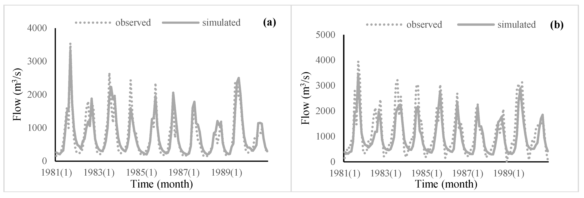
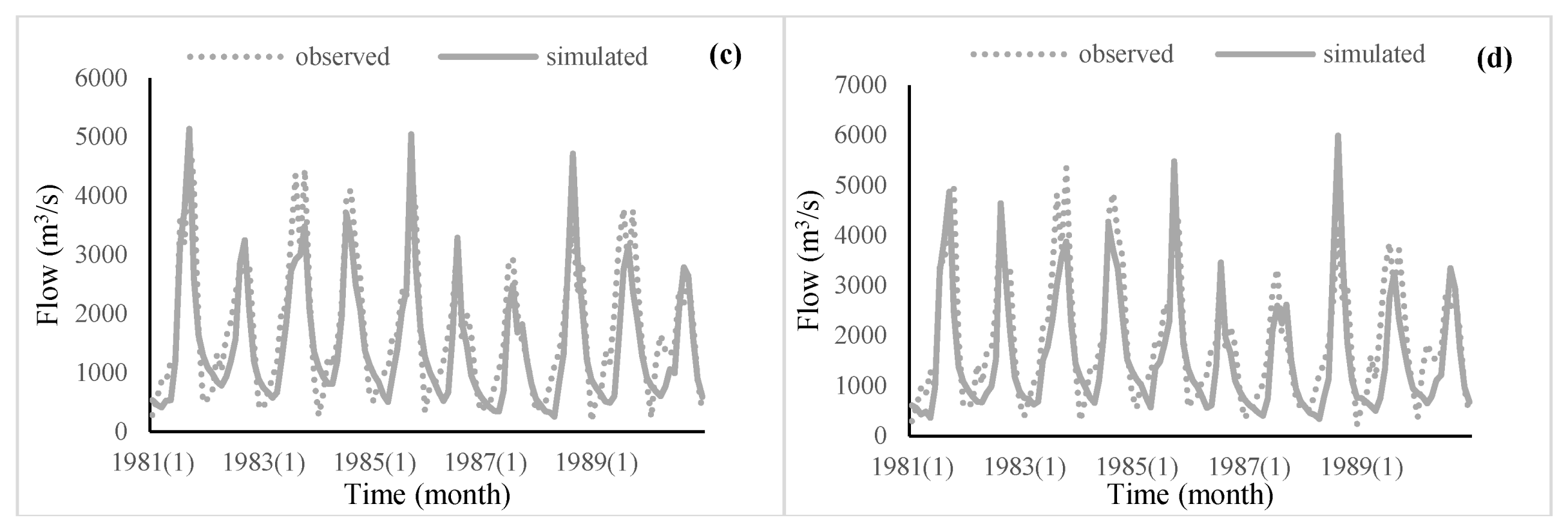
If the absolute value of RE between runoff simulation and observation values is less than 20%, NS is greater than 0.6 and R² is greater than 0.6, it is considered that the established SWAT model can be applied to simulate the runoff of the study area [43,44,45,46].

Figure 4 and Figure 5 and

Table 4. Determination coefficient (R²), Nash–Sutcliffe coefficient (NS), relative error (RE) values for calibration and validation period.

Hydrological Station	Calibration Period (1970–1980)			Validation Period (1981–1990)
	R2	NS	RE(%)	R2	NS	RE(%)
Tangnaihai	0.72	0.68	6.81	0.82	0.82	−4.54
Toudaoguai	0.74	0.66	18.22	0.77	0.71	15.67
Sanmenxia	0.76	0.72	5.47	0.78	0.73	13.02
Lijin	0.77	0.74	7.67	0.74	0.68	15.72

display the correlation between monthly observations and simulated flow values of Tangnaihai, Toudaoguai, Sanmenxia and Lijin Hydrological stations during the calibration period (1970–1980) and validation period (1980–1990). The R² values of the four hydrological stations in the calibration period and validation period are all greater than 0.7, RE values are all less than 20%, and NS values are all greater than 0.6, so the SWAT model can well simulate the monthly runoff changes of Tangnaihai, Toudaoguai, Sanmenxia and Lijin hydrological stations in the calibration period and validation period.

3.2. Future Land Use Simulation of the Yellow River Basin

In this study, the land cover map of the Yellow River Basin in 2050 is simulated by IDRISI 17.2 software, which is developed by Clark University. The software includes more than 300 practical and professional modules, such as remote sensing image processing, GIS analysis, decision analysis, spatial analysis, land use change analysis, global change monitoring, suitability assessment mapping, geostatistical analysis, and cellular automata land dynamic change trend prediction. The main steps are as follows:

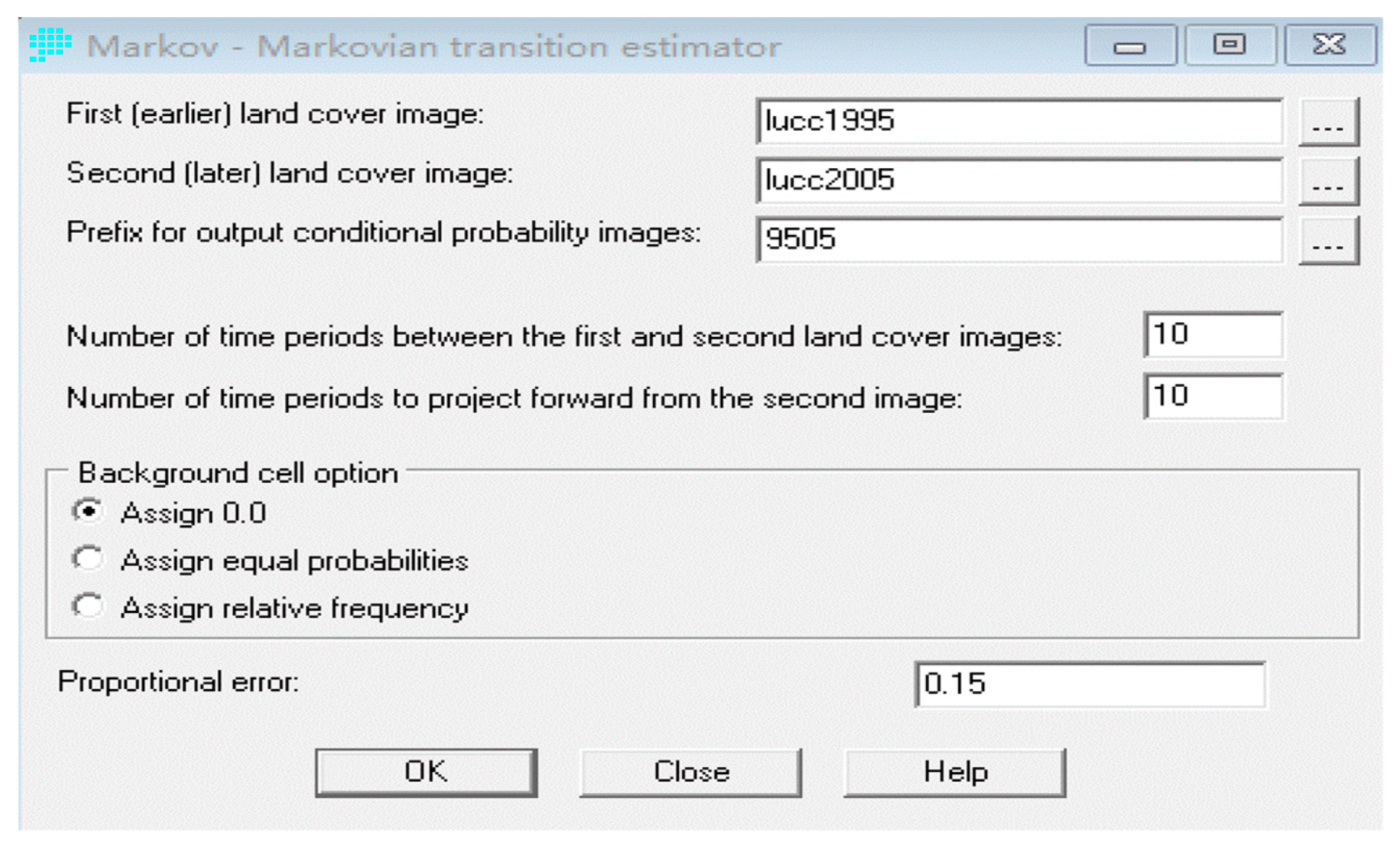
(1) Taking the land use data of the Yellow River Basin in 1995 and 2005 as the initial year and the last year, the probability transfer matrix of land use from 1995 to 2005 can be obtained by the Markov module in the IDRISI 17.2 software (Figure 6);

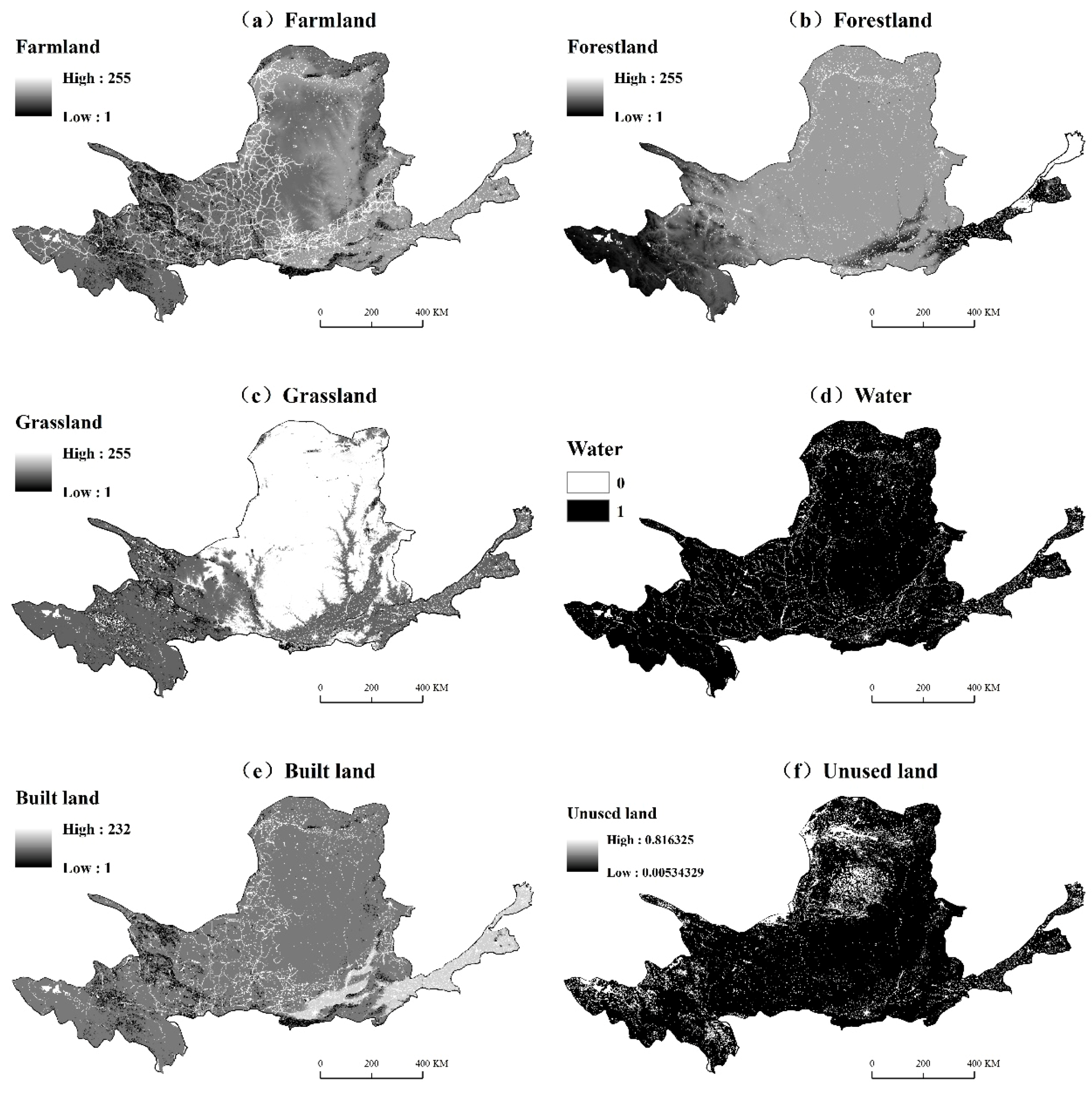
(2) The transition suitability maps are generated for the six land cover classes by the Multi-Objective Decision Wizard module (Figure 7). The rules are as follows: ①Built land: elevation <500 m is the most suitable, the elevation is suitable for 500–1500 m, and elevation >1500 m indicates poor suitability; slope between 0° and 5° is the most suitable, slope between 5° and 15° is suitable, and slope >15° indicates poor suitability; distance to road <500 m is the most suitable, distance to road between 500 m and 1000 m is suitable, and distance to road >1 km indicates poor suitability. ②Farmland: elevation <500 m is the most suitable, the elevation is suitable for 500–1500 m, and elevation >1000 m indicates poor suitability; slope within 0–5° is the most suitable, slope with 5–15° indicates poor suitability, and >15° is unsuitable; distance to highway <1 km is the most suitable, distance to road between 1 km and 3 km is suitable, and distance to road >3 km indicates weak suitability. ③The conversion of water to other land types is prohibited; ④Elevation is the main constraint factor of forestland and grassland. Unused land can be converted to other land types at will. Finally, the transfer suitability maps of six land types are generated (Figure 8);

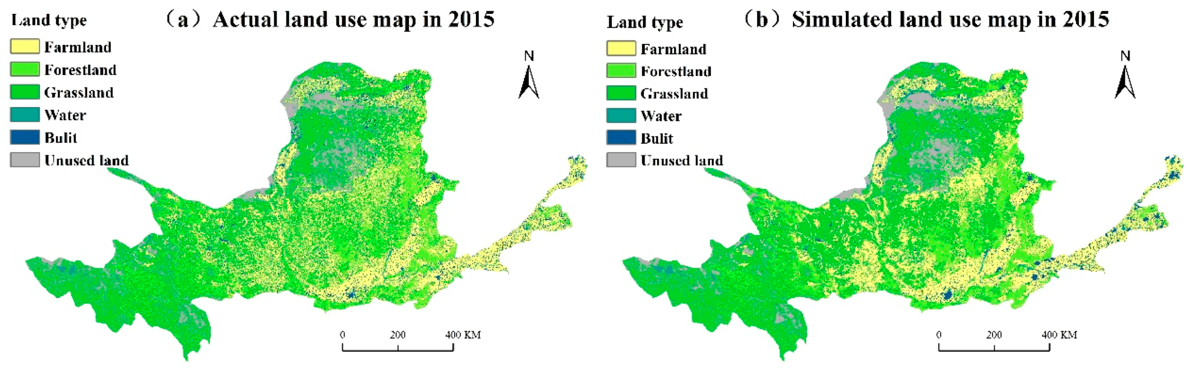
(3) Taking the land use data of 2005 as the initial data, the probability transfer matrix from 1995 to 2005 and suitability maps (Figure 8) are input into the CA-Markov model. The 5 × 5 neighborhood filter is selected as the neighborhood definition. The unit size is set as 1000 m × 1000 m and the cycle is set to 10 times. The land use data of the Yellow River Basin in 2015 can be simulated (Figure 9);

(4) The CROSSTAB module of IDRISI 17.2 software is used to calculate the Kappa coefficient (Figure 10), and the result is 0.82, indicating that the CA-Markov model can well simulate the land cover change in the Yellow River Basin;

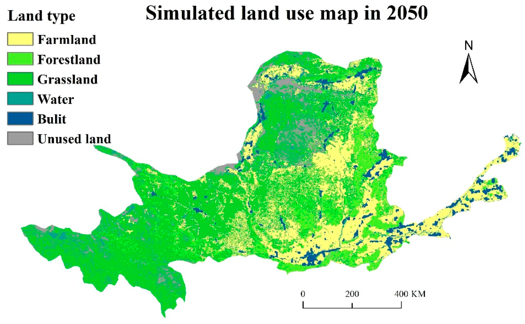
(5) Taking the land use data of 2015 as the initial data, the probability transfer matrix from 1980 to 2015 (

Table 5. The probability transfer matrix of land use from 2015 to 2050 under the status quo continuation scenario.

Year	Land Type	2050
		Farmland	Forestland	Grassland	Water	Built Land	Unused Land
2015	Farmland	0.7461	0.0324	0.1048	0.0129	0.0975	0.0063
	Forestland	0.0509	0.8128	0.1014	0.0043	0.0182	0.0124
	Grassland	0.1157	0.039	0.7346	0.0098	0.0185	0.0824
	Water	0.2242	0.0104	0.0667	0.6218	0.0254	0.0514
	Built land	0.233	0.0038	0.026	0.007	0.7271	0.0031
	Unused land	0.039	0.0059	0.2839	0.0147	0.0132	0.6433

) and suitability maps (Figure 8) are input into the CA-Markov model. The 5 × 5 neighborhood filter is selected as the neighborhood definition. The cycle is set to 35 times. The land use data of the Yellow River Basin in 2050 can be simulated (Figure 11).

Table 6. Comparison of land types percentage in the Yellow River Basin in 2015 and in 2050 under status quo continuation scenario.

Land Type	2015	2050
		Percentage (%)	Variation (%)
Farmland	24.63	26.28	1.65
Forestland	14.14	12.35	−1.79
Grassland	47.25	45.98	−1.27
Water	2.02	1.85	−0.17
Built land	3.13	5.12	1.99
Unused land	8.83	8.42	−0.40

shows the difference of land types percentage in the Yellow River Basin in 2015 and in 2050 under status quo continuation scenario. The area percentages of farmland, forestland, grassland, water, built land and unused land in the Yellow River Basin in 2050 under the status quo continuation scenario are 26.28%, 12.35%, 45.98%, 1.85%, 5.12% and 8.42%, respectively, and the change ranges are 1.65%, −1.79%, −1.27%, −0.17%, 1.99% and −0.40%, respectively, compared with 2015.

3.3. Future Runoff Simulation of the Yellow River Basin

In this section, we focus on the average value of simulated flow results based on the five global climate models. In this paper, the SWAT model is used to simulate the runoff of the Yellow River Basin in the middle of the 21st century (2040–2060) under the combined action of representative concentration path (RCP) scenarios and Land use change (LUC) scenarios (RCP-LUC). The differences between the runoff of the Yellow River Basin in the future (2040–2060) and the base period (1970–1990) are analyzed from four aspects: average runoff, seasonal runoff proportion, monthly runoff proportion and high extreme runoff (Q95). Among them, the monthly runoff value is ranked from low to high, and the value ranked at 95% is the high extreme runoff (Q95). Q95 extreme runoff indicates the 95th percentile of the monthly flow distribution, which can represent the occurrence of flood disasters in a basin [47,48,49].

3.3.1. Average Runoff Change

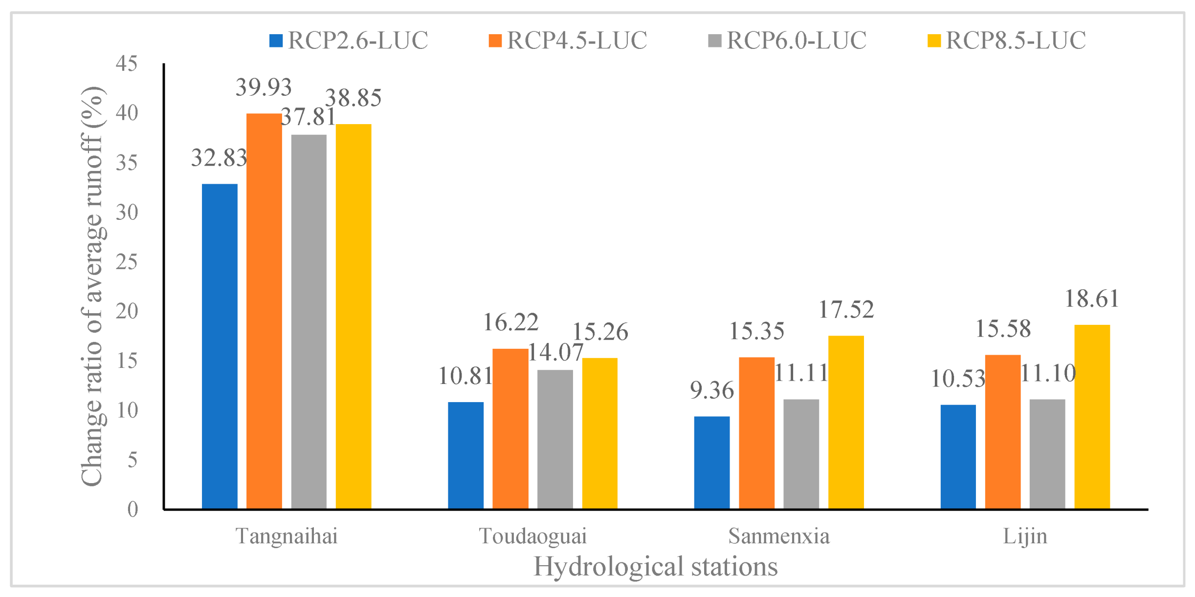
The differences between the average runoff of the four hydrological stations in the middle of the 21st century (2040–2060) and the base period (1970–1990) are displayed in Figure 12. The average runoff of Tangnaihai, Toudaoguai, Sanmenxia and Lijin stations under four RCP-LUC scenarios tends to increase compared with the base period. Compared with different RCP-LUC scenarios, the order of average runoff increment of Tangnaihai and Toudaoguai hydrological stations is RCP4.5-LUC>RCP8.5-LUC>RCP6.0-LUC>RCP2.6-LUC; the order of average runoff increment of Sanmenxia and Lijin hydrological stations is RCP8.5-LUC>RCP4.5-LUC>RCP2.6-LUC>RCP6.0-LUC.

Compared with the future runoff simulation results under RCP scenarios in the existing studies [11,12], it is found that the average runoff in the future under the RCP-LUC scenario is greater, which indicates that land use data input into the SWAT model will have a great impact on future runoff simulation results.

3.3.2. Seasonal Runoff Proportion Change

Table 7. The differences between the seasonal runoff proportion in the future period and the base period of the four hydrological stations (%).

Hydrological Station	Scenario	Spring	Summer	Autmun	Winter
Tangnahai	RCP2.6-LUC	−4.11	0.78	0.28	3.05
	RCP4.5-LUC	−4.19	0.81	0.36	3.02
	RCP6.0-LUC	−4.01	0.60	0.27	3.13
	RCP8.5-LUC	−4.39	0.89	0.54	2.97
Toudaoguai	RCP2.6-LUC	−6.34	−0.64	0.77	6.20
	RCP4.5-LUC	−6.27	−1.09	1.06	6.30
	RCP6.0-LUC	−6.09	−1.21	0.93	6.37
	RCP8.5-LUC	−6.34	−0.87	1.04	6.17
Sanmenxia	RCP2.6-LUC	−7.18	1.33	0.28	5.57
	RCP4.5-LUC	−7.11	0.85	0.40	5.86
	RCP6.0-LUC	−6.96	0.67	0.56	5.72
	RCP8.5-LUC	−6.98	1.09	0.10	5.79
Lijin	RCP2.6-LUC	−6.52	2.44	−1.09	5.17
	RCP4.5-LUC	−6.47	2.00	−0.90	5.36
	RCP6.0-LUC	−6.30	1.77	−0.77	5.30
	RCP8.5-LUC	−6.46	2.54	−1.29	5.21

displays the differences between the proportion of seasonal runoff in the future period (2040–2060) and the base period (1970–1990). Compared with the base period, the runoff proportion of Tangnaihai and Sanmenxia hydrological stations in spring tends to decrease, and it increases in summer, autumn and winter. The runoff proportion of Toudaoguai hydrological station in spring and summer decreases, and increases in autumn and winter. The runoff proportion of Lijin station in spring and autumn decreases, and increases in summer and winter. To sum up, under the RCP-LUC scenario, the spring runoff proportion of the four hydrological stations shows a decreasing trend, and the winter runoff proportion tends to increase. The variation trend of runoff proportion in summer and autumn at four hydrological stations is different.

3.3.3. Monthly Runoff Proportion Change

The differences between the monthly runoff proportion of the four hydrological stations in the future period (2040–2060) and the base period (1970–1990) are shown in

Table 8. The differences between the monthly runoff proportion in the future period and the base period of the four hydrological stations (%).

Hydrological Stations	Scenarios	January	February	March	April	May	June	July	August	September	October	November	December
Tangnaihai	RCP2.6-LUC	1.05	0.91	0.41	−1.25	−3.28	−1.90	−0.71	3.39	1.43	−1.07	−0.08	1.09
	RCP4.5-LUC	1.06	0.89	0.35	−1.23	−3.31	−2.05	−0.85	3.71	1.64	−1.15	−0.13	1.07
	RCP6.0-LUC	1.07	0.94	0.42	−1.21	−3.22	−1.89	−0.85	3.35	1.37	−1.06	−0.04	1.12
	RCP8.5-LUC	1.05	0.85	0.24	−1.39	−3.25	−1.64	−0.82	3.34	1.58	−0.97	−0.07	1.07
Toudaoguai	RCP2.6-LUC	2.18	1.13	−1.34	−1.49	−3.50	−3.23	−1.13	3.72	1.08	−0.92	0.62	2.89
	RCP4.5-LUC	2.21	1.17	−1.34	−1.45	−3.48	−3.31	−1.41	3.63	1.39	−0.94	0.61	2.92
	RCP6.0-LUC	2.24	1.19	−1.28	−1.40	−3.41	−3.14	−1.34	3.27	1.16	−0.89	0.66	2.95
	RCP8.5-LUC	2.17	1.11	−1.39	−1.51	−3.44	−3.05	−1.20	3.38	1.25	−0.84	0.63	2.88
Sanmenxia	RCP2.6-LUC	2.16	0.60	−2.03	−2.02	−3.13	−1.08	−0.42	2.84	1.06	−0.86	0.08	2.81
	RCP4.5-LUC	2.26	0.71	−1.95	−1.96	−3.20	−1.25	−0.65	2.75	1.17	−0.88	0.11	2.90
	RCP6.0-LUC	2.22	0.68	−1.97	−1.96	−3.03	−0.95	−0.59	2.21	1.26	−0.75	0.05	2.83
	RCP8.5-LUC	2.23	0.68	−1.96	−1.92	−3.11	−1.17	−0.44	2.70	0.96	−0.93	0.07	2.87
Lijin	RCP2.6-LUC	2.08	0.66	−1.67	−1.86	−2.99	−1.12	−0.04	3.53	0.85	−1.46	−0.48	2.42
	RCP4.5-LUC	2.15	0.76	−1.61	−1.81	−3.05	−1.23	−0.07	3.29	1.03	−1.42	−0.51	2.45
	RCP6.0-LUC	2.14	0.72	−1.60	−1.79	−2.91	−0.91	−0.03	2.71	1.04	−1.28	−0.53	2.44
	RCP8.5-LUC	2.11	0.69	−1.66	−1.82	−2.98	−1.18	0.20	3.52	0.77	−1.49	−0.57	2.41

. Compared with the base period, the monthly proportion runoff of the four hydrological stations in the Yellow River Basin all changed in the middle of the 21st century. The monthly runoff proportion of Tangnaihai, Toudaoguai, Sanmenxia and Lijin hydrological stations in the middle of the 21st century (2040–2060) tends to decrease in April, May, June, July and October. The monthly runoff proportion of the four hydrological stations tends to increase in January, February, August, September and December.

3.3.4. Q95 Extreme Runoff Change

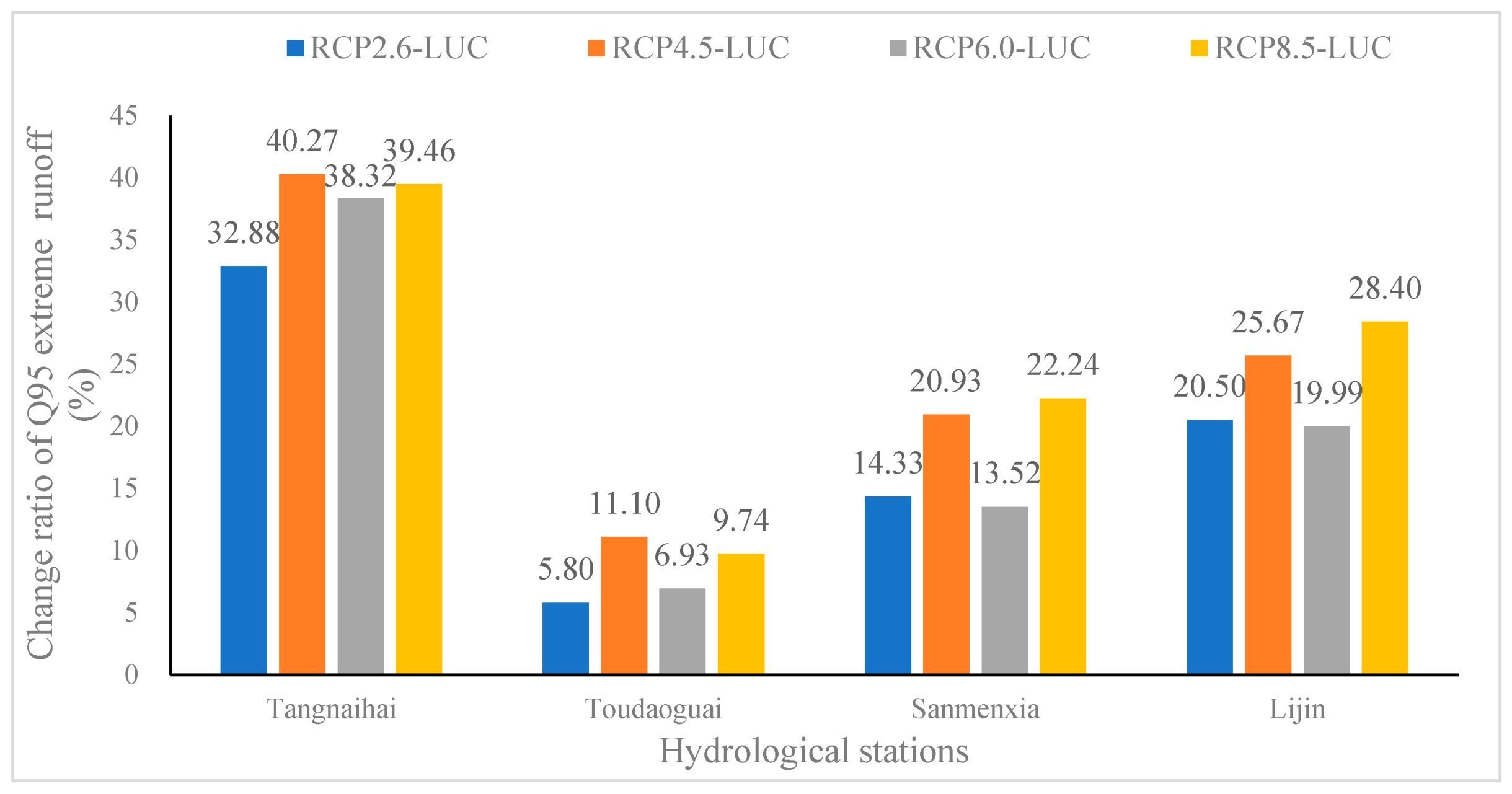
The differences between the Q95 extreme runoff of four hydrological stations in the middle of the 21st century (2040–2060) and the base period (1970–1990) are shown in Figure 13. Compared with the base period, the Q95 extreme runoff of Tangnaihai, Toudaoguai, Sanmenxia and Lijin stations all increased obviously, indicating that the probability of flood disasters in the Yellow River Basin will increase in the future period.

Compared with different RCP-LUC scenarios, the order of Q95 extreme runoff increment of Tangnaihai and Toudaoguai hydrological stations is RCP4.5-LUC>RCP8.5-LUC>RCP6.0-LUC>RCP2.6-LUC; the order of Q95 extreme runoff increment of Sanmenxia and Lijin hydrological stations is RCP8.5-LUC>RCP4.5-LUC>RCP2.6-LUC>RCP6.0-LUC. In a word, Tangnaihai and Lijin hydrological stations have the highest probability of flood disasters under the RCP4.5-LUC scenario, while Sanmenxia and Lijin hydrological stations have the highest probability of flood disasters under the RCP8.5-LUC scenario.

Compared with the future runoff simulation results under RCP scenarios in the existing studies [11,12], it is found that the Q95 extreme runoff in the future under the RCP-LUC scenario is greater, which indicates that existing studies have underestimated the risk of flood disasters in the future.

4. Discussion

4.1. Uncertainty of SWAT and CA-Markov Model on Runoff Simulation

Although the SWAT and CA-Markov models have rigorous theoretical basis and complex structure, there are still some uncertainties when using mathematical formulas to describe the process of runoff generation and land change. In the follow-up study, in order to reduce the uncertainties of the model on the future runoff simulation results, multiple models can be used to simulate the future runoff change (such as VIC and SWAT model) and future land use maps (such as CA-Markov and FLUS model) of the Yellow River Basin.

4.2. Uncertainty of Parameter Calibration on Runoff Simulation

In this paper, the monthly runoff data of Tangnaihai, Toudaoguai, Sanmenxia and Lijin in the Yellow River Basin are verified by the SUFI2 algorithm in SWAT-CUP software. However, there is still some uncertainty between the simulation results and the actual observation data. During the verification period (1981–1990), the relative errors between the monthly flow observation values and simulated values of Tangnaihai, Toudaoguai, Sanmenxia and Lijin hydrological stations in the Yellow River Basin are −4.54%, 15.67%, 13.02% and 15.72%, respectively. These parameters will lead to some uncertainties on runoff simulation results in the future. In the follow-up study, we need to collect more data such as urban water, industrial water, agricultural water and water conservancy dam construction, so as to establish a more accurate SWAT model.

4.3. Uncertainty of Global Climate Models on Runoff Simulation

For the study of climate change on river runoff, the main uncertainty is the global climate model data [50]. These uncertainties are highly correlated with the corresponding structure, parameters and spatial resolution of the global climate model [51]. The differences between the average runoff and Q95 extreme runoff of the five global climate models in the middle of the 21st century and the base period are shown in

Table 9. The differences between future average runoff, Q95 extreme runoff and base period of the four hydrological stations (%).

Global Climate Model	Hydrological Station	RCP2.6-LUC		RCP4.5-LUC		RCP6.0-LUC		RCP8.5-LUC
		Average Runoff	Q95 Extreme Runoff	Average Runoff	Q95 Extreme Runoff	Average Runoff	Q95 Extreme Runoff	Average Runoff	Q95 Extreme Runoff
GFDL-ESM2M	Tangnaihai	50.51	53.79	63.28	60.29	67.96	65.55	65.91	64.08
	Toudaoguai	25.79	34.13	42.30	43.81	44.90	50.15	48.79	51.38
	Sanmenxia	36.70	52.80	59.63	67.08	53.58	63.83	76.00	87.34
	Lijin	40.86	64.60	62.34	77.66	52.84	76.82	79.17	100.60
HadGEM2-ES	Tangnaihai	34.72	20.64	38.26	24.76	23.65	19.99	23.46	11.70
	Toudaoguai	8.84	−4.13	4.21	−6.55	−11.08	−10.91	−4.73	−15.44
	Sanmenxia	5.02	3.54	−1.72	4.66	−22.52	−10.53	−6.75	−5.14
	Lijin	9.83	12.53	0.89	10.74	−22.42	−5.76	−2.53	0.02
IPSL-CM5A-LR	Tangnaihai	65.55	51.68	71.85	59.48	72.76	65.66	92.52	77.30
	Toudaoguai	28.72	14.05	32.58	19.13	33.00	16.30	46.61	28.33
	Sanmenxia	18.04	17.19	13.72	14.02	19.59	18.50	36.37	27.59
	Lijin	17.19	19.66	12.49	15.86	19.40	23.58	35.55	32.15
MIROC-ESM-CHEM	Tangnaihai	31.43	17.50	52.17	34.18	34.86	23.94	40.38	27.52
	Toudaoguai	3.41	−6.03	19.71	6.31	4.94	−3.89	6.66	−1.60
	Sanmenxia	0.46	5.30	23.08	16.76	2.51	3.78	6.24	7.12
	Lijin	0.20	6.79	19.43	18.78	0.22	7.82	2.96	8.49
NorES1-M	Tangnaihai	33.07	20.80	33.17	22.64	19.55	16.47	19.47	16.68
	Toudaoguai	4.24	−9.04	3.71	−7.19	−7.22	−17.01	−4.66	−13.98
	Sanmenxia	−4.06	−7.17	−2.14	2.11	−13.89	−8.00	−9.42	−5.68
	Lijin	−1.13	−1.08	−1.33	5.33	−13.23	−2.51	−6.44	0.72

.

The variation range of the average runoff and Q95 extreme runoff of Tangnaihai, Toudaoguai, Sanmenxia and Lijin hydrological stations is very large, which shows that different climate models will lead to great difference in runoff simulation results of the Yellow River Basin in the future. However, using multiple global climate model data can reduce the uncertainty of runoff simulation in the future [50,51]. In this study, only five sets of global climate model data are used as the basic data. In the follow-up study, we will use more climate model data to estimate future runoff.

4.4. Uncertainty of Land Use Simulation on Runoff Simulation

The CROSSTAB module of IDRISI 17.2 software was used to calculate the Kappa coefficient and the result is 0.82, which will lead to some uncertainties on land use simulation results in the future. In the follow-up study, we will establish a more accurate CA-Markov model to simulate land use data of the Yellow River Basin. In addition, in the follow-up study, it is necessary to simulate the future land use under the scenarios of ecological protection, status quo continuation and rapid urbanization, and analyze the impact of different land use change scenarios on future runoff.

5. Conclusions

This paper simulated the future runoff change in the Yellow River Basin under the combined effect of land use and climate change (RCP-LUC) based on CA-Markov and SWAT, and analyzed the changes in the average runoff, Q95 extreme runoff and intra-annual runoff distribution under the RCP-LUC scenario. The conclusions were as follows:

(1) Compared with the base period (1970–1990), the average runoff of the Yellow River Basin shows an increasing trend in the future period (2040–2060), and the probability of flood disasters also tends to increase.

(2) Compared with the future runoff simulation results under the RCP scenario in the existing studies [11,12], it is found that the average runoff and Q95 extreme runoff in the future under the RCP-LUC scenario are greater, which indicates that existing studies have underestimated the risk of flood disasters in the future.

(3) Compared with the base period, the spring runoff proportion of the four hydrological stations in the Yellow River Basin in the future period (2040–2060) shows a decreasing trend, which increases the risk of drought in spring. The winter runoff proportion tends to increase, and the variation trend of runoff proportion in summer and autumn at four hydrological stations is different.

(4) Compared with the base period (1970–1990), the monthly runoff proportion of the four hydrological stations in the Yellow River Basin in the future period (2040–2060) tends to decrease in April, May, June, July and October, and tends to increase in January, February, August, September and December.

References

- Liu, C.; Liu, X.; Tian, W.; Xie, J. Ecological Protection and High-Quality Development of the Yellow River Basin Urgently need to Solve the Water Shortage Problem. Yellow River 2020, 42, 6–9. (In Chinese) [Google Scholar]
- Xu, Z.X.; Zhao, F.F.; Li, J.Y. Response of stream flow to climate change in the headwater catchment of the Yellow River basin. Quat. Int. 2009, 208, 62–75. [Google Scholar] [CrossRef]
- Zhang, L.; Yang, X. Applying a Multi-Model Ensemble Method for Long-Term Runoff Prediction under Climate Change Scenarios for the Yellow River Basin, China. Water 2018, 10, 301. [Google Scholar] [CrossRef] [Green Version]
- Wang, Z.P.; Tian, J.C.; Feng, K.P. Response of Runoff in Ningxia Section of Yellow River Basin of China to Climate Changes. Appl. Ecol. Environ. Res. 2019, 17, 7855–7863. [Google Scholar] [CrossRef]
- Kim, J.; Choi, J.; Choi, C.; Park, S. Impacts of changes in climate and land use/land cover under IPCC RCP scenarios on streamflow in the Hoeya River Basin, Korea. Sci. Total Environ. 2013, 452–453, 181–195. [Google Scholar] [CrossRef]
- Mehdi, B.; Ludwig, R.; Lehner, B. Evaluating the impacts of climate change and crop land use change on streamflow, nitrates and phosphorus: A modeling study in Bavaria. J. Hydrol. Reg. Stud. 2015, 4, 60–90. [Google Scholar] [CrossRef] [Green Version]
- Pan, S.; Liu, D.; Wang, Z.; Zhao, Q.; Zou, H.; Hou, Y.; Liu, P.; Xiong, L. Runoff Responses to Climate and Land Use/Cover Changes under Future Scenarios. Water 2017, 9, 475. [Google Scholar] [CrossRef] [Green Version]
- Oliveira, V.; Mello, C.; Viola, M.R.; Srinivasan, R. Land-use change impacts on the hydrology of the upper grande river basin, brazil. Cerne 2018, 24, 334–343. [Google Scholar] [CrossRef]
- Li, L.; Hao, Z.; Wang, J.; Wang, Z.; Yu, Z. Impact of Future Climate Change on Runoff in the Head Region of the Yellow River. J. Hydrol. Eng. 2008, 13, 347–354. [Google Scholar] [CrossRef]
- Li, L.; Shen, H.; Dai, S.; Xiao, J.; Shi, X. Response of runoff to climate change and its future tendency in the source region of Yellow River. J. Geogr. Sci. 2012, 22, 431–440. [Google Scholar] [CrossRef]
- Wei, J.; Chang, J.; Chen, L. Runoff change in upper reach of Yellow River under future climate change based on VIC model. J. Hydroelectr. Eng. 2016, 35, 65–74. (In Chinese) [Google Scholar]
- Lu, W.; Wang, W.; Shao, Q.; Yu, Z.; Hao, Z.; Xing, W.; Yong, B.; Li, J. Hydrological projections of future climate change over the source region of Yellow River and Yangtze River in the Tibetan Plateau: A comprehensive assessment by coupling RegCM4 and VIC model. Hydrol. Process. 2018, 32, 2096–2117. [Google Scholar] [CrossRef]
- Gao, P.; Geissen, V.; Ritsema, C.J.; Mu, X.; Wang, F. Impact of climate change and anthropogenic activities on stream flow and sediment discharge in the Wei River basin, China. Hydrol. Earth Syst. Sci. 2013, 17, 961–972. [Google Scholar] [CrossRef] [Green Version]
- Julian, M.M.; Ward, P.J. Assessment of the effects of climate and land cover changes on river discharge and sediment yield, and an adaptive spatial planning in the Jakarta region. Nat. hazards 2014, 73, 507–530. [Google Scholar]
- Astuti, I.S.; Sahoo, K.; Milewski, A.; Mishra, D.R. Impact of land use land cover (LULC) change on surface runoff in an increasingly urbanized tropical watershed. Water Resour. Manag. 2019, 33, 4087–4103. [Google Scholar] [CrossRef]
- Barnett, T.P.; Pierce, D.W.; Hidalgo, H.G.; Bonfils, C.; Santer, B.D.; Das, T.; Bala, G.; Wood, A.W.; Nozawa, T.; Mirin, A.A. Human-induced changes in the hydrology of the western United States. Science 2008, 319, 1080–1083. [Google Scholar] [CrossRef] [PubMed] [Green Version]
- Lorencová, E.; Frélichová, J.; Nelson, E.; Vačkářd, D. Past and future impacts of land use and climate change on agricultural ecosystem services in the Czech Republic. Land Use Policy 2013, 33, 183–194. [Google Scholar] [CrossRef]
- Zhang, H.; Meng, C.; Wang, Y.; Wang, Y.; Li, M. Comprehensive evaluation of the effects of climate change and land use and land cover change variables on runoff and sediment discharge. Sci. Total Environ. 2020, 702, 134401. [Google Scholar] [CrossRef]
- Zhang, H.; Yang, L.; Zhang, X. Study on the Economic and Social Development Indicators in the Yellow River Basin. Yellow River 2013, 35, 11–13. (In Chinese) [Google Scholar]
- Ma, D.; Deng, H.; Yin, Y.; Wu, S.; Zheng, D. Sensitivity of arid/humid patterns in china to future climate change under a high-emissions scenario. J. Geogr. Sci. 2019, 29, 29–48. [Google Scholar] [CrossRef] [Green Version]
- Zhao, J.; Xia, H.; Yue, Q.; Wang, Z. Spatiotemporal variation in reference evapotranspiration and its contributing climatic factors in China under future scenarios. Int. J. Climatol. 2020, 40, 3813–3831. [Google Scholar] [CrossRef]
- Hay, L.E.; Wilby, R.L.; Leavesley, G.H. A Comparison of Delta Change and Downscaled GCM Scenarios for Three Mountainous Basins in the United States. JAWRA J. Am. Water Resour. Assoc. 2000, 36, 387–397. [Google Scholar] [CrossRef]
- Li, L.; Xu, H.; Chen, X.; Simonovic, S.P. Streamflow Forecast and Reservoir Operation Performance Assessment Under Climate Change. Water Resour. Manag. 2010, 24, 83–104. [Google Scholar] [CrossRef]
- Ren, J.; Peng, S.; Cao, Y.; Huo, X.; Chen, Y. Spatiotemporal Distribution Characteristics of Climate Change in the Loess Plateau from 1901 to 2014. J. Nat. Resour. 2018, 33, 83–95. (In Chinese) [Google Scholar]
- Guan, D.J.; Li, H.F.; Inohae, T.; Su, W.; Hokao, K. Modeling urban land use change by the integration of cellular automaton and Markov model. Ecol. Model. 2011, 222, 3761–3772. [Google Scholar] [CrossRef]
- Araya, Y.H. Analysis and modeling of urban land cover change in Setubal and Sesimbra Portugal. Remote Sens. 2010, 2, 1549–1563. [Google Scholar] [CrossRef] [Green Version]
- Susanna, T.Y.; Tong, Y.S.; Ranatunga, T.; Jie, H.; Yang, J. Predicting plausible impacts of sets of climate and landusechange scenarios on water resources. Appl. Geogr. 2012, 32, 477–489. [Google Scholar]
- Abbaspour, K.C.; Rouholahnejad, E.; Vaghefi, S.; Srinivasan, R.; Yang, H.; Kløve, B. A continental-scale hydrology and water quality model for Europe: Calibration and uncertainty of a high-resolution large-scale SWAT model. J. Hydrol. 2015, 524, 733–752. [Google Scholar] [CrossRef] [Green Version]
- Easton, Z.M.; Fuka, D.R.; Walter, M.T.; Cowan, D.M.; Schneiderman, E.M.; Steenhuisa, T.S. Re-conceptualizing the soil and water assessment tool (SWAT) model to predict runoff from variable source areas. J. Hydrol. 2008, 348, 279–291. [Google Scholar] [CrossRef]
- Lv, Z.; Zuo, J.; Rodriguez, D. Predicting of Runoff Using an Optimized SWAT-ANN: A Case Study. J. Hydrol. Reg. Stud. 2020, 29, 100688. [Google Scholar] [CrossRef]
- Mehta, V.M.; Mendoza, K.; Daggupati, P.; Srinivasan, R.; Rosenberg, N.J.; Deb, D. High-resolution Simulations of Decadal Climate Variability Impacts on Water Yield in the Missouri River Basin with the Soil and Water Assessment Tool (SWAT). J. Hydrometeorol. 2015, 17, 2455–2476. [Google Scholar] [CrossRef]
- Sun, R.; Zhang, X.; Sun, Y.; Zheng, D.; Fraedrich, K. SWAT-Based Streamflow Estimation and Its Responses to Climate Change in the Kadongjia River Watershed, Southern Tibet. J. Hydrometeorol. 2013, 14, 1571–1586. [Google Scholar] [CrossRef]
- Panagopoulos, Y.; Makropoulos, C.; Baltas, E.; Mimikou, M. SWAT parameterization for the identification of critical diffuse pollution source areas under data limitations. Ecol. Model. 2011, 222, 3500–3512. [Google Scholar] [CrossRef]
- Pulighe, G.; Bonati, G.; Colangeli, M.; Traverso, L.; Napoli, M. Predicting Streamflow and Nutrient Loadings in a Semi-Arid Mediterranean Watershed with Ephemeral Streams Using the SWAT Model. Agronomy 2020, 10, 2. [Google Scholar] [CrossRef] [Green Version]
- Zeiger, S.L.; Hubbart, J.A. A SWAT model validation of nested-scale contemporaneous stream flow, suspended sediment and nutrients from a multiple-land-use watershed of the central USA. Sci. Total Environ. 2016, 572, 232–243. [Google Scholar] [CrossRef]
- Zhang, L.; Liu, Y.; Cai, D.; Fan, K.; Ma, X. Comparison and Applicability of Automatic Calibration Methods of the Parameters in SWAT Model—A Case Study of the Middle and Upper Reaches of the Jinghe River Watershed. China Rural Water Hydropower 2016, 11, 76–81. (in Chinese). [Google Scholar]
- Chen, H.; Luo, Y.; Potter, C.; Moran, P.J.; Grieneisen, M.L.; Zhang, M. Modeling pesticide diuron loading from the san joaquin watershed into the sacramento-san joaquin delta using SWAT. Water Res. 2017, 121, 374–385. [Google Scholar] [CrossRef] [PubMed]
- Abbaspour, K.C.; Yang, J.; Maximov, I.; Siber, R.; Bogner, K.; Mieleitner, J.; Zobrist, J.; Srinivasan, R. Modelling hydrology and water quality in the pre-alpine/alpine thur watershed using SWAT. J. Hydrol. 2007, 333, 413–430. [Google Scholar] [CrossRef]
- MCkay, M.D.; Beckma, R.J.; Conover, W.J. A comparision of three methods for selelcting valuses of input variables in the analysis of output from a computer code. Am. Stat. Assoc. Am. Soc. Qual. 2000, 42, 55–61. [Google Scholar]
- Abbaspour, K.C. SWAT-CUP: SWAT Calibration and Uncertainty Programs—A User Manual; Swiss Federal Institute of Aquatic Science and Technology, Eawag: Dübendorf, Switzerland, 2015. [Google Scholar]
- Wu, J.; Zhang, H.; Yang, X. SWAT-Based Runoff Simulation and Runoff Responses to Climate Change in the Headwaters of the Yellow River, China. Atmosphere 2019, 10, 509. [Google Scholar] [CrossRef] [Green Version]
- Xu, H.; Taylor, R.G.; Xu, Y. Quantifying uncertainty in the impacts of climate change on river discharge in sub-catchments of the Yangtze and Yellow River Basins, China. Hydrol. Earth Syst. Sci. 2011, 15, 333–344. [Google Scholar] [CrossRef] [Green Version]
- Chen, Y.; Xu, C.Y.; Chen, X.; Xu, Y.; Yin, Y.; Gao, L.; Liu, M. Uncertainty in simulation of land-use change impacts on catchment runoff with multi-timescales based on the comparison of the HSPF and SWAT models. J. Hydrol. 2019, 573, 486–500. [Google Scholar] [CrossRef]
- Ruan, H.; Zou, S.; Yang, D.; Wang, Y.; Yin, Z.; Lu, Z.; Li, F.; Xu, B. Runoff Simulation by SWAT Model Using High-Resolution Gridded Precipitation in the Upper Heihe River Basin, Northeastern Tibetan Plateau. Water 2017, 9, 866. [Google Scholar] [CrossRef] [Green Version]
- Zhang, L.; Meng, X.; Wang, H.; Yang, M. Simulated Runoff and Sediment Yield Responses to Land-Use Change Using the SWAT Model in Northeast China. Water 2019, 11, 915. [Google Scholar] [CrossRef] [Green Version]
- Wang, Y.; Zhu, S.; Yuan, L.; Deng, R. An automatic parameter calibration method for the SWAT model in runoff simulation. River Res. Appl. 2020, 36, 1321–1333. [Google Scholar] [CrossRef]
- Dinpashoh, Y.; Singh, V.P.; Biazar, S.M.; Kavehkar, S. Impact of climate change on streamflow timing (case study: Guilan Province). Theor. Appl. Climatol. 2019, 138, 65–76. [Google Scholar] [CrossRef]
- Tharme, R.E. A Global Perspective on Environmental Flow Assessment: Emerging Trends in the Development and Application of Environmental Flow Methodologies for Rivers. River Res. Appl. 2003, 19, 397–441. [Google Scholar] [CrossRef]
- Van Vliet, M.T.H.; Franssen, W.H.P.; Yearsley, J.R.; Ludwig, F.; Haddeland, I.; Lettenmaier, D.P.; Kabat, P. Global River Discharge and Water Temperature under Climate Change. Glob. Environ. Chang-Hum. Policy Dimens. 2013, 23, 450–464. [Google Scholar] [CrossRef]
- Teng, J.; Vaze, J.; Chiew, F.H.S.; Wang, B.; Perraud, J.M. Estimating the Relative Uncertainties Sourced from GCMs and Hydrological Models in Modeling Climate Change Impact on Runoff. J. Hydrometeorol. 2012, 13, 122–139. [Google Scholar] [CrossRef]
- Yan, D.; Werners, S.E.; Ludwig, F.; Huang, H.Q. Hydrological response to climate change: The Pearl River, China under different RCP scenarios. J. Hydrol. Reg. Stud. 2015, 4, 228–245. [Google Scholar] [CrossRef] [Green Version]
Figure 1.
The location of hydrological and meteorological stations in and around the Yellow River Basin.
Figure 2.
Sub basins division of the Yellow River Basin.
Figure 3.
Soil types in the Yellow River Basin (Note: the number after the abbreviation of soil type indicates that the soil type is the same, but the soil physical parameters are inconsistent).
Figure 4.
Monthly flow observation and simulation values of Tangnaihai (a), Toudaoguai (b), Sanmenxia (c) and Lijin (d) during calibration period (1970–1980).
Figure 5.
Monthly flow observation and simulation values of Tangnaihai (a), Toudaoguai (b), Sanmenxia (c) and Lijin (d) during validation period (1981–1990).
Figure 6.
Calculation of land use probability transfer matrix by Markov module.
Figure 7.
Constructing suitability atlas with Multi-Objective Decision Wizard module.
Figure 8.
Suitability maps of farmland (a), forestland (b), grassland (c), water (d), built land (e) and unused land (f).
Figure 9.
Comparison between simulated and actual land use maps in 2015.
Figure 10.
Calculation of Kappa coefficient by CROSSTAB module.
Figure 11.
Simulated land use maps of the Yellow River Basin in 2050.
Figure 12.
The differences between the average runoff in the future period and the base period of the four hydrological stations.