Interconnected Risk Contributions: A Heavy-Tail Approach to Analyze U.S. Financial Sectors

Abstract

This paper investigates the dynamic evolution of tail risk interdependence among U.S. banks, financial services and insurance sectors. Life and non-life insurers have been considered separately to account for their different characteristics. The tail risk interdependence measurement framework relies on the multivariate Student-t Markov switching (MS) model and the multiple-conditional value-at-risk (CoVaR) (conditional expected shortfall (CoES)) risk measures introduced in Bernardi et al. (2013), accounting for both the stylized facts of financial data and the contemporaneous multiple joint distress events. The Shapley value methodology is then applied to compose the puzzle of individual risk attributions, providing a synthetic measure of tail interdependence. Our empirical investigation finds that banks appear to contribute more to the tail risk evolution of all of the remaining sectors, followed by the financial services and the insurance sectors, showing that the insurance sector significantly contributes as well to the overall risk. We also find that the role of each sector in contributing to other sectors’ distress evolves over time according to the current predominant financial condition, implying different interdependence strength.

1. Introduction

For a long period of time in most countries, there has been a distinct separation among insurance companies, banks and financial institutions providing diversified financial services, so that events in one sector usually had little or negligible effects on the others. However, in more recent years, the barriers among institutions have been partly dismantled, resulting in much closer interconnections and overlaps between them and their activities. As extensively documented in Cummins and Weiss [1,2], since the 1970s, insurance companies have been expanding their activities further beyond traditional instruments consisting of insurance coverages and capital accumulation products. During recent years, insurance companies have been investing in corporate bonds and equity, have become proprietaries of mutual funds and have entered the market of investment management by providing structured financial products in direct competition with the banking sector. On the other hand, banks and financial institutions providing general financial services have engaged in a variety of non-core activities, such as insurance underwriting, traditionally devoted to insurers. Diversified financial services firms now offer banking, insurance and investment products, becoming very complicated structured financial firms belonging to the so-called “shadow banking system”, which consists of financial intermediaries that provide banking-like services without access to central bank liquidity or explicit government credit guarantees; see, e.g., Pozsar et al. [3]. Direct and indirect dependencies among participants of a financial market have contributed to the spread of malfunctions from one failing financial institution to the remaining market participants, providing serious adverse effects to the real economy. As an example, the expansion by the insurance corporation American International Group (AIG) of the core activity into the credit default swaps (CDS) market has been highlighted as one of the major causes of its collapse, bailout and quasi-nationalization at the end of September 2008; see, e.g., Harrington [4] and Cummins and Weiss [1]. The involvement of AIG and Monoline bond issuers in CDS markets for the purposes of synthetic securitization being undertaken by banks brought hitherto unconnected sectors into close proximity; see Markose et al. [5]. Furthermore, the expansion of the activity into the securitization market by issuing products like mortgage-backed securities and asset-backed securities have increased the vulnerability of financial companies to crisis episodes. The recent Global Financial Crisis (GFC) has witnessed the fragility of the U.S. financial system to systemic events, like the housing bubble burst in mid-2007. The collapse of the global housing bubble and the consequent uncertainty about the value of the linked structured securities, led to sharp declines in the value of securities tied to real estate and to the freezing of the interbank lending and the commercial paper market. The spillover of the housing and mortgage-backed security problems into the broader credit market, the stock market and the real economy is an example of how systemic risk can be triggered by the liquidity risk and by the exposure to the housing market through securitization.

This paper aims to investigate and fill the gap of inter-sector analysis and to address the problem of assessing the tail risk interdependence among different sectors composing the financial system, namely banking, insurance and diversified financial services. The idea is to stress the importance of mapping out the relationships between all of those sectors, highlighting the degree of their dependence to extreme events affecting one or more of them. The latest financial crisis has created a deep interest in measuring the tail risk interdependence among institutions in order to evaluate the spillover effects on the real economy. The interdependence among institutions has been recognized to be a key requirement in gauging the vulnerability of the market or institutions to systemic events, further beyond the exposure to common shocks. Recent research focuses on the degree of interconnectedness within the financial industry. Using the principal component analysis and the Granger causality test, Billio et al. [6] analyze stock price data on hedge funds, banks, brokers and insurers for the period 1994–2008. They find that financial institutions have become significantly linked during the period 2001–2008 and, more interestingly, an asymmetric interconnection relationship between banks and insurers, on the one hand, and hedge funds and brokers, on the other hand. Adams et al. [7] instead develop a state-dependent sensitivity value-at-risk approach being able to quantify the direction, size and duration of risk spillovers among systemically important financial institutions. Their analysis considers a system of quantile regressions involving the entire panel of institutions, conditional on the relevant state of the system. Their results confirm that commercial banks and hedge funds play a relevant role in the transmission of shocks to other financial institutions. The same results are confirmed by Acharya et al. [8] using the systemic expected shortfall risk measure. They also find that insurance firms are overall the least systemically risky and that the top three systemically risky insurers were heavily involved in providing financial guarantees for structured products in the credit derivatives market. Hautsch et al. [9] propose a network analysis of the tail interdependence among institutions. In their empirical analysis for the pre-GFC crisis period, they find that only two insurance companies, American International Group and Cincinnati Financial Corp, were qualified as systemically relevant, while most of the remaining insurance companies were considered to be of a low level of systemic importance.

In the recent literature, sectors, like insurance, which has been considered for a long time safer than banks in their core activities, have been showing a significantly altered risk profile due to the aforementioned expansion of the business to non-core activities, which may affect the overall risk amount of the system. Billio et al. [6] and Acharya et al. [8] reveal that insurance firms can be a source of systemic risk, while Cummins and Weiss [1] and Harrington [4] find that the interconnectedness among banks and insurance companies has grown considerably in recent years and that the systemic relevance of insurance companies is mainly related to their expansion of non-core activities as well as to the reinsurance crisis. Using different approaches, Bernal et al. [10], Brechmann et al. [11], Chen et al. [12] and Podlich and Wedow [13] find that the impact of banks on insurers is stronger and of longer duration than the impact of insurers on banks for the U.S. market.

In the same spirit as the previous literature, one relevant contribution of our analysis is to investigate the extreme interdependence of the banking and insurance industries. To analyze in depth the risk contribution of insurers with different core activities, we segment the insurance sector into life and non-life indices. As far as we know, this is the first attempt to consider separately life and non-life insurers in a risk contribution framework. This latter aspect is of great interest, as life and non-life insurers may differ for their exposure to risk, as well as for the composition of their investment portfolios, which is important for systemic risk management; see, e.g., Cummins and Weiss [1,2] and Harrington [4]. Concerning the first aspect, Cummins and Weiss [1] find that non-life insurance companies are more exposed than life insurance companies to catastrophe risks. Life insurers instead face higher exposure to the housing market and asset liquidity risk, in comparison to non-life insurance companies. Regarding the composition of their respective portfolios, both life and non-life insurers are long-term bond investors, even if they invest with different average bond maturities. Moreover, as documented in Cummins and Weiss [1,2], the percentage of assets invested in equity stocks in 2012 were much higher for non-life than life insurance. Concerning the composition of balance sheets, we observe that asset and liabilities maturities are both long-term for insurers, whereas banks have short-term liabilities and long-term assets. This maturity mismatch, characteristic of banks’ asset and liabilities, constitutes a major source of systemic risk for the banking sector compared to the insurance one. Moreover, most of the bank liabilities are instantaneously payable, while non-life insurance liabilities are not immediately due, and life insurance companies usually have only a small proportion of their liabilities payable at any time. Concerning their investment horizons, those are usually longer for insurance companies than for banks and other financial services. This characteristic largely contributes to increasing their riskiness profiles, since insurance risk usually propagates over a longer time horizon than systemic risk in the banking system.

Throughout the paper, the tail interdependence analysis relies on a multiple extension of the conditional value-at-risk (CoVaR) recently introduced in the financial literature by Adrian and Brunnermeier [14]. The CoVaR approach measures the value-at-risk of an institution conditional on another individual institution being in financial distress. The literature on co-movement risk measures has proliferated during the last few years (see, e.g., Bernardi et al. [15]; Bernal et al. [10]; Castro and Ferrari [16]; Girardi and Ergün [17]; Jäger–Ambrożewicz [18]; and Sordo et al. [19]). Bisias et al. [20] provide an extensive and up to date survey of the systemic risk measures that have been recently proposed. However, when dealing with highly interconnected systems, it is possible that several institutions jointly experience financial distress events at the same time. The CoVaR risk measure cannot account for the possibility of multiple joint distress events, since it considers only one institution’s distress at a time. Underestimation of the simultaneous occurrence of interdependent rare events and the consequent bias in evaluating the transmission of risks among sectors may cause misleading policy reactions by the authorities. To account for possible underestimation problems, recently, Bernardi et al. (2013) [21] and Cao [22] have proposed an extension of the CoVaR and conditional expected shortfall (CoES), the so-called multiple-CoVaR and multiple-CoES, which consider joint occurrences of extreme losses as conditioning events. Here, following Bernardi et al. [21], we propose a multivariate model-based approach to measure the dynamic evolution of tail risk interdependence within the financial sector and its major constituents. The proposed methodology evaluates the contribution of each financial sector to the total risk of the remaining ones accounting for the fact that several sectors may experience extreme tail risk events at the same time. In order to implement this idea, we consider a sequence of cooperative games, where each one of the four sectors, banks, diversified financial services, life and non-life insurance acts, in turn, as the “main”sector with respect to which the risk of any other distress events affecting the remaining market participants is evaluated. The approach is based on a multivariate Student-t Markov switching (MS) model being able to capture different dynamic risk profiles, through the inclusion of latent states, as well as to account for several stylized facts, like asymmetry, heavy tails, non-linearity and persistence of extreme observations. Those features are crucial in financial returns time series analysis (see, e.g., Bulla [23]; Granger and Ding [24,25]; and Rydén et al. [26]). This way, we contribute to evaluating risk measures that are intrinsically dynamic, since they rely on time-varying loadings of individual risk factors represented by the value-at-risks. The resulting dynamic evolution over time provides important monitoring tools for the market-based macro-prudential or financial stability regulation. Moreover, since we evaluate the proposed risk measures on the Markov switching (MS) predictive distribution, we provide a forward-looking approach to tail risk interdependence assessment.

The empirical strategy employed in the paper to assess the extreme tail interdependence of banking, diversified financial services, life and non-life insurance sectors consists of monitoring each sectors’ total risk evolution using the aforementioned dynamic MS model and the associated multiple risk measures. The dynamic latent class model in conjunction with the considered multiple risk measures provide an early warning indicator of the overall state the financial system is experiencing. Empirically, we observe that the dynamic evolution of the total risk for the different sectors provide a signal that usually anticipates the subsequent financial crisis. Furthermore, measuring the contribution of each sector to the riskiness of the remaining ones, using the cross-comparison of the multiple-$\Delta \mathrm{CoVaR}$ and the multiple-$\Delta \mathrm{CoES}$, which are the multiple generalization of the $\Delta \mathrm{CoVaR}$ and the $\Delta \mathrm{CoES}$ of Adrian and Brunnermeier [14], we detect the amount of extreme tail interactions among sectors. The Shapley [27] value methodology is then applied to finally attribute the total risk shares to each sector. The resulting Shapley values multiple-ΔCoVaR and multiple-ΔCoES provide, for each sector, the shares of total risk of all of the remaining ones. In the empirical part, we analyze the effective interdependence among financial sectors using weekly data on the Dow Jones U.S. banks, the Dow Jones U.S. financial services and the Dow Jones life and non-life insurance indices, for the period from 1 January 1992 to 28 June 2013.

Our empirical findings suggest that each financial sector significantly impacts on each other during crisis periods, as well as during more stable phases. When comparing the contribution of each financial industry, banks appear to contribute more to the tail risk evolution of all of the remaining sectors, followed by financial services and the insurance industry. These results confirm that insurance sector contributes as well to other sectors’ overall risk. In addition to this, we find that the role of each sector in contributing to other sectors’ distress evolves over time according to the current predominant financial condition. We also show that banks and financial services are more extremely interdependent than insurance sectors and that the strength of interdependence between banks and insurance is more evident after the GFC of 2008. Finally, comparing life and non-life insurance, we find that they are highly interdependent, both during crisis periods, as well as during phases of financial stability, but the overall level of interdependence decreases after the end of the 2008 crisis.

The remainder of the paper is structured as follows. Section 2 introduces the Student-t MS model. Section 3 provides the definition of the multiple risk measures and details the Shapley value methodology used throughout the paper. Section 4 describes our empirical results, while Section 5 provides a detailed discussion of our empirical findings. Section 6 concludes.

2. The Model

In this section, we provide a brief description of the MS model with particular emphasis on the Student-t component distribution. The choice of this model is motivated by its attitude to represent well the financial time series dynamics capturing the underlying structure of the observations, like heavy tails, asymmetry and non-linear dependence. Moreover, the hidden Markov structure is able to identify periods of crisis, as well as phases of financial stability. Those characteristics are particularly relevant when the main objective is to measure and manage financial or systemic risks. In particular, the MS model dynamics allows us to quantify the evolution over time and over states of the dependence among indexes’ returns. For a deeper review of MS models, see, e.g., Cappé et al. [28], Zucchini and MacDonald [29] and Dymarski [30]. Recent applications of MS models to financial market returns may be found in Bulla [23], Amisano and Geweke [31] and Geweke and Amisano [32]. Recently, Bernardi et al. [21] analyzed the implications of multivariate Student-t MS models to evaluate extreme tail risk interconnectedness among financial markets participants in the bank sector. In what follows, we shortly describe the model they propose, to which we refer throughout the paper.

Let $\left\{{\mathbf{\text{Y}}}_t,t=1,\cdots ,T\right\}$ denote a sequence of multivariate observations, where ${\mathbf{\text{Y}}}_t=\{y_{1,t},y_{2,t},\cdots ,y_{p,t}\}\in {\mathbb{R}}^p$, and $\left\{S_t,t=1,2,\cdots ,T\right\}$ is a Markov chain defined on the state space $\{1,2,\cdots ,L\}$. In the MS model setting, the conditional distribution for the observation process $\left\{{\mathbf{\text{Y}}}_t\right\}$ depends only on the latent state at time t, i.e.,

$$f\left({\mathbf{\text{Y}}}_t={\mathbf{\text{y}}}_t\mid {\mathbf{\text{Y}}}_{1:t-1}={\mathbf{\text{y}}}_{1:t-1},S_{1:t}=s_{1:t}\right)=f\left({\mathbf{\text{Y}}}_t={\mathbf{\text{y}}}_t\mid S_t=s_t\right)$$

where ${\mathbf{\text{Y}}}_{1:t-1}=\left({\mathbf{\text{Y}}}_1,{\mathbf{\text{Y}}}_2,\cdots ,{\mathbf{\text{Y}}}_{t-1}\right)$, $S_{1:t}=\left(S_1,S_2,\cdots ,S_t\right)$ and ${\mathbf{\text{y}}}_{1:t-1}$, $s_{1:t-1}$ denote the realizations up to time $t-1$ of the observed and latent processes, respectively. The unobservable Markov process $\left\{S_t\right\}$ satisfies the following Markov property:

$$\mathbb{P}\left(S_t=s_t\mid S_{1:t-1}=s_{1:t-1}\right)=\mathbb{P}\left(S_t=s_t\mid S_{t-1}=s_{t-1}\right)=\mathbf{\text{Q}}$$

where $\mathbf{\text{Q}}={\left\{q_{j,l}\right\}}_{j,l=1,2,\cdots ,L}$ is the Markovian transition matrix with $q_{j,l}=\mathbb{P}\left(S_t=j\mid S_{t-1}=l\right)$, indicating the probability that state j is visited at time t given that at time $t-1$, the chain was visiting state l. We also indicate with $\mathsf{\delta }=\left({\mathsf{\delta }}_1,{\mathsf{\delta }}_2,\cdots ,{\mathsf{\delta }}_L\right)$ the vector initial probabilities of being in state l, $\mathbb{P}\left(S_1=l\right)={\mathsf{\delta }}_l$, for all $l=1,2,\cdots ,L$.

Whenever we deal with financial time series, it is important to account for the well-known stylized facts, as well as possible time varying dependence structures among extreme events, which are relevant in assessing economic risks. Those reasons motivate our assumption of multivariate Student-t distribution for modeling the observed process, i.e.,

$${\mathbf{\text{Y}}}_t\mid S_t=s_t\sim {\mathcal{T}}_p\left({\mathsf{\mu }}_{s_t}{,}_{{\sum }_{st}},{\nu }_{s_t}\right)$$

(1)

where $\left({\mathsf{\mu }}_l,{\mathbf{\sum }}_l,{\nu }_l\right)$, $l=1,2,\cdots ,L$ denote location, scale and degrees of freedom parameters, respectively.

To make inference on the unknown model parameters, we consider the expectation-maximization (EM) algorithm of Dempster et al. [33]. Details about the specific implementation of the EM algorithm under the multivariate Student-t component density assumption are provided in Bernardi et al. [21].

The multiple risk measures considered in the paper to assess risk interdependence are calculated on the predictive distribution of the observables in order to get a forward-looking risk quantification. Let $h>0$ denote the forecasting horizon and ${\mathcal{I}}_t$ denote the information set up to time t, i.e., ${\mathcal{I}}_t=\left\{y_{1:t},s_{1:t}\right\}$, the predictive distribution of MS models is a finite mixture of component specific predictive distributions:

$$\mathbb{P}\left({\mathbf{\text{y}}}_{t+h}\mid {\mathcal{I}}_t\right)=\sum _{l=1}^L{\pi }_l^{\left(h\right)}f\left({\mathbf{\text{y}}}_{t+h}\mid S_{t+h}=l\right)$$

(2)

with mixing weights:

$${\pi }_l^{\left(h\right)}=\sum _{j=1}^L{\mathbf{Q}}_{j,l}^h\mathbb{P}\left(S_t=j\mid {\mathcal{I}}_t\right)$$

(3)

where ${\mathbf{Q}}_{l,j}^h$ is the $\left(j,l\right)$-th entry of the Markovian transition matrix $\mathbf{\text{Q}}$ to the power h and $\mathbb{P}\left(S_t=j\mid {\mathcal{I}}_t\right)$ is the filtered probability of state $j=1,2,\cdots ,L$ at time t. In what follows, we fix the predictive horizon h equal to one, i.e., $h=1$.

3. Risk Measurement Framework

The main objective of the paper is to evaluate how the simultaneous interdependence among multiple distress events affects the overall health level of insurance, banks and other financial service sectors. To measure the tail co-movement between those institutions, we refer to the multiple-CoVaR and multiple-CoES introduced in Bernardi et al. [21], who generalized the Adrian and Brunnermeier’s CoVaR and CoES to account for multiple contemporaneous distress events. Then, to compose the puzzle of individual risk attribution, we rely on the Shapley value methodology introduced by Shapley [27] in the context of cooperative game theory. In this way, we are able to measure the contribution of a given financial sector to the riskiness of a different sector being contemporaneously linked to all of the remaining ones, which may themselves experience extreme losses. Moreover, as already mentioned, evaluating risk measures on MS models allows one to capture the risk evolution driven by different financial and economics conditions. In the following subsection, we defined the multiple risk measures, while in Section 3.2, we detail how the Shapley value method applies in the context of extreme tail interdependence measurement. In what follows, we suppress the time dependence in the notation for convenience.

3.1. Multiple Risk Measures

Let $\mathcal{S}=\left\{1,2,\cdots ,p\right\}$ be a set of p institutions, we assume that the conditioning event is a set of d institutions under distress indexed by ${\mathcal{J}}_{\mathsf{D}}=\left\{j_1,j_2,\cdots ,j_d\right\}\subset {}_{}{}^d\mathbb{C}_{p-1}^{}$, where ${}_{}{}^d\mathbb{C}_{p-1}^{}$ is the set of all possible combinations of $p-1$ elements of class d, with $d=1,2,\cdots ,p-1$. Moreover, assuming that institution $i\in \mathcal{S}$ with $i\notin {\mathcal{J}}_{\mathsf{D}}$ and ${\mathcal{J}}_{\mathsf{N}}=\overline{{\mathcal{J}}_{\mathsf{D}}}$ is the set of institutions being in the “normal” state, we define the “multiple-CoVaR”, ${\text{CoVaR}}_{i|{\mathcal{J}}_{\mathsf{D}}}^{{\tau }_1|{\tau }_2}$, where ${\tau }_1,{\tau }_2\in \left(0,1\right)$ are given confidence levels, as follows:

Definition 1. 

Let $\mathbf{\text{Y}}=\left(Y_1,Y_2,\cdots ,Y_i,\cdots ,Y_p\right)$ be the vector of institution returns; then, ${\mathrm{CoVaR}}_{i|{\mathcal{J}}_{\mathsf{D}}}^{{\tau }_1|{\tau }_2}$ is the value-at-risk of institution $i\in \mathcal{S}$ at confidence level ${\tau }_1$, conditional on the set of institutions ${\mathcal{J}}_{\mathsf{D}}$ being at their individual ${\mathrm{VaR}}_{{\tau }_2}$ level ${\widehat{\mathbf{\text{y}}}}_{{\mathcal{J}}_{\mathsf{D}}}^{{\tau }_2}=\left({\widehat{y}}_{j_1}^{{\tau }_2},{\widehat{y}}_{j_2}^{{\tau }_2},\cdots ,{\widehat{y}}_{j_d}^{{\tau }_2}\right)$ and the set of institutions ${\mathcal{J}}_{\mathsf{N}}=\overline{{\mathcal{J}}_{\mathsf{D}}}$ being at their individual ${\mathrm{VaR}}_{0.5}$ level ${\widehat{\mathbf{\text{y}}}}_{{\mathcal{J}}_{\mathsf{N}}}^{0.5}=\left({\widehat{y}}_{j_{d+1}}^{0.5},{\widehat{y}}_{j_{d+2}}^{0.5},\cdots ,{\widehat{y}}_{j_{p-1}}^{0.5}\right)$, i.e., ${\mathrm{CoVaR}}_{i|{\mathcal{J}}_{\mathsf{D}}}^{{\tau }_1|{\tau }_2}$ satisfies the following equation:

$$\mathbb{P}\left(Y_i\le {\mathrm{CoVaR}}_{i|{\mathcal{J}}_{\mathsf{D}}}^{{\tau }_1|{\tau }_2}{\mid }_{{\mathbf{\text{Y}}}_{\mathcal{J}\mathsf{D}}}={\widehat{\mathbf{\text{y}}}}_{{\mathcal{J}}_{\mathsf{D}}}^{{\tau }_2}{,}_{{\mathbf{\text{Y}}}_{\mathcal{J}\mathsf{N}}}={\widehat{\mathbf{\text{y}}}}_{{\mathcal{J}}_{\mathsf{N}}}^{0.5}\right)={\tau }_1,\forall i=1,2,\cdots ,p$$

(4)

The lack of subadditivity property of the value-at-risk suggests to introduce, in addition to the CoVaR, the conditional expected shortfall (CoES), defined by Adrian and Brunnermeier [14] as the expected shortfall (ES) evaluated on the conditional distribution of $Y_i$ given $Y_j$, for two different institutions i and j, with $i\ne j$. The following definition characterizes the extension of CoES to the multiple-CoES, accounting for multiple contemporaneous distress events.

Definition 2. 

Let $\mathbf{\text{Y}}=\left(Y_1,Y_2,\cdots ,Y_i,\cdots ,Y_p\right)$ be the vector of institution returns; then, the ${\mathrm{CoES}}_{i|{\mathcal{J}}_{\mathsf{D}}}^{{\tau }_1|{\tau }_2}$ is the expected shortfall of institution $i\in \mathcal{S}$, conditional on the set of institutions ${\mathcal{J}}_{\mathsf{D}}$ being at their individual ${\mathrm{ES}}_{{\tau }_2}$ level ${\widehat{\psi }}_{{\mathbf{\text{y}}}_{{\mathcal{J}}_{\mathsf{D}}}}\left({\widehat{\mathbf{\text{y}}}}_{{\mathcal{J}}_{\mathsf{D}}}^{{\tau }_2}\right)=\left({\widehat{\psi }}_{y_{j_1}}\left({\widehat{y}}_{j_1}^{{\tau }_2}\right),{\widehat{\psi }}_{y_{j_2}}\left({\widehat{y}}_{j_2}^{{\tau }_2}\right),\cdots ,{\widehat{\psi }}_{y_{j_d}}\left({\widehat{y}}_{j_d}^{{\tau }_2}\right)\right)$ and the set of institutions ${\mathcal{J}}_{\mathsf{N}}$ being at their individual ${\mathrm{ES}}_{0.5}$ level ${\widehat{\psi }}_{y_{{\mathcal{J}}_{\mathsf{N}}}}\left({\widehat{\psi }}_{{\mathcal{J}}_{\mathsf{N}}}^{0.5}\right)=\left({\widehat{\psi }}_{y_{j_{d+1}}}\left({\widehat{y}}_{j_{d+1}}^{0.5}\right),{\widehat{\psi }}_{y_{j_{d+2}}}\left({\widehat{y}}_{j_{d+2}}^{0.5}\right),\cdots ,{\widehat{\psi }}_{y_{j_{p-1}}}\left({\widehat{y}}_{j_{p-1}}^{0.5}\right)\right)$, with ${\widehat{\psi }}_{y_j}\left({\widehat{y}}_j^{\tau }\right)\equiv {\mathrm{ES}}_{\tau }\left(Y_j\right)$, $\forall j=1,2,\cdots ,d$, and can be defined in the following way:

$${\mathrm{CoES}}_{i|{\mathbf{\text{Y}}}_{\mathcal{J}\mathsf{D}}}^{{\tau }_1|{\tau }_2}\equiv \mathbb{E}\left(Y_i\mid Y_i\le {\widehat{y}}_i^{{\tau }_1}{,}_{{\mathcal{J}}_{\mathsf{D}}}={\widehat{\psi }}_{{}_{{\mathcal{J}}_{\mathsf{D}}}}\left({\widehat{\psi }}_{{\mathcal{J}}_{\mathsf{D}}}^{{\tau }_2}\right){,}_{{\mathbf{\text{Y}}}_{\mathcal{J}\mathsf{N}}}={\widehat{\psi }}_{{\mathbf{\text{y}}}_{{\mathcal{J}}_{\mathsf{N}}}}\left({\widehat{\psi }}_{{\mathcal{J}}_{\mathsf{N}}}^{0.5}\right)\right)$$

(5)

$\forall i=1,2,\cdots ,p$.

Analytical formulae for the multiple-CoVaR and multiple-CoES defined in Equations (4) and (5), under the multivariate Student-t MS model are provided in Bernardi et al. [21].

In order to quantify the marginal contribution of individual institutions, we consider the multiple-ΔCoVaR (${\Delta }^{\mathsf{M}}\text{CoVaR}$) and the multiple-ΔCoES (${\Delta }^{\mathsf{M}}\text{CoES}$) as straightforward generalization of the ΔCoVaR and ΔCoES of Adrian and Brunnermaier [14], defined as follows:

$$\begin{array}{cc}\hfill {\Delta }^{\mathsf{M}}{\mathrm{CoVaR}}_{i|{\mathcal{J}}_{\mathsf{D}}}^{{\tau }_1|{\tau }_2}& ={\mathrm{CoVaR}}_{i|{\mathcal{J}}_{\mathsf{D}}}^{{\tau }_1|{\tau }_2}-{\mathrm{CoVaR}}_{i|{\mathcal{J}}_{\mathsf{D}}\cup {\mathcal{J}}_{\mathsf{N}}}^{{\tau }_1|{\tau }_2}\hfill \end{array}$$

(6)

$$\begin{array}{cc}\hfill {\Delta }^{\mathsf{M}}{\mathrm{CoES}}_{i|{\mathcal{J}}_{\mathsf{D}}}^{{\tau }_1|{\tau }_2}& ={\mathrm{CoES}}_{i|{\mathcal{J}}_{\mathsf{D}}}^{{\tau }_1|{\tau }_2}-{\mathrm{CoES}}_{i|{\mathcal{J}}_{\mathsf{D}}\cup {\mathcal{J}}_{\mathsf{N}}}^{{\tau }_1|{\tau }_2}\hfill \end{array}$$

(7)

for $i=1,2,\cdots ,p$.

Since different sets of institutions belonging to the conditioning distress events qualify different measures of risk contribution, to compose the puzzle of overall risk attribution to each institution, we apply the Shapley value methodology initially proposed by Shapley [27] in the field of cooperative games. The idea of applying the Shapley value methodology to the systemic risk attribution has been previously considered by Tarashev et al. [34], Cao [22] and Bernardi et al. [21]. The next section details the implementation of the cooperative game theory in our risk measurement framework.

3.2. Shapley Value Methodology

The Shapley [27] value methodology is used to efficiently evaluate the financial risk of each institution or portfolio shared by each of the remaining participants to the financial system. In particular, for each institution $i=1,2,\cdots ,p$, a cooperative game is denoted by the couple $\left({\vartheta }_i,p-1\right)$, where p is the total number of institutions in the market and ${\vartheta }_i:2^{p-1}⟶\mathbb{R}$ is the loss function of individual i assigning the cost ${\vartheta }_i\left(\mathcal{H}\right)$ to each coalition $\mathcal{H}\subset \mathcal{S}\setminus \left\{i\right\}$, provided that ${\vartheta }_i\left(\varnothing \right)=0$, $\forall i=1,2,\cdots ,p$. In our risk measurement framework, the loss function ${\vartheta }_i,i=1,2,\cdots ,p$ coincides with the multiple-ΔCoVaR or the multiple-ΔCoES, and it assigns to each of the $2^{p-1}$ possible groups of institutions $\mathcal{H}$ its marginal contribution to the total risk in such a way that ${\vartheta }_i\left(\mathcal{S}\setminus \left\{i\right\}\right)$ is the total risk of institution $i\in \mathcal{S}$. In the cooperative game theory framework, the function ${\vartheta }_i\left(·\right)$ should be sub-additive, such that the contribution of a union of disjoint coalitions is less than the sum of the coalition’s separate values, i.e., for all disjoint partitions $\left({\mathcal{H}}_j,{\mathcal{H}}_k\right)\in \mathcal{S}\setminus \left\{i\right\}$ with $j\ne k$, such that ${\mathcal{H}}_j\cap {\mathcal{H}}_k=\varnothing$, ${\theta }_i\left({\mathcal{H}}_j\cup {\mathcal{H}}_k\right)\le {\theta }_i\left({\mathcal{H}}_j\right)+\theta \left({\mathcal{H}}_k\right)$. By definition, the subadditivity property holds when the loss function inherits a coherent risk measure.

The Shapley value is one of the possible ways to distribute the total risk of institution $i\in \mathcal{S}$, i.e., ${\vartheta }_i\left(\mathcal{S}\setminus \left\{i\right\}\right)$, among all of the remaining institutions belonging to the financial system, assuming that they all collaborate. In particular, the Shapley value of institution $j\in \mathcal{S}\setminus \left\{i\right\}$, denoted by ${\mathrm{ShV}}_i\left(j\right)$, determines the amount of institution j’s risk contribution on institution i and satisfies the “individual rationality condition”, i.e., ${\mathrm{ShV}}_i\left(j\right)\ge {\vartheta }_i\left(\left\{j\right\}\right)$, $\forall i,j\in \mathcal{S}$, with $j\ne i$, where ${\vartheta }_i\left(\left\{j\right\}\right)$ is the marginal risk contribution of institution j if it does not cooperate, and the “collective rationality condition”, i.e., ${\sum }_{j=1}^p{\mathrm{ShV}}_i\left(j\right)={\vartheta }_i\left(\mathcal{S}\right)$, $\forall i\in \mathcal{S}$. The Shapley values are obtained as:

$${\mathrm{ShV}}_i\left(j\right)=\frac{{\sum }_{\mathcal{H}\subset \mathcal{S}\setminus \left\{i,j\right\}}\left|\mathcal{H}\right|!\left(|\mathcal{S}\setminus \left\{i\right\}|-|\mathcal{H}|-1\right)!\left[{\vartheta }_i\left(\mathcal{H}\cup \left\{j\right\}\right)-{\vartheta }_i\left(\mathcal{H}\right)\right]}{|\mathcal{S}\setminus \left\{i\right\}|!}$$

(8)

for $i,j=1,2,\cdots ,p$ with $j\ne i$, where for any given sector $i=1,2,\cdots ,p$, coalition $\mathcal{H}\subset \mathcal{S}\setminus \left\{i,j\right\}$, ${\vartheta }_i\left(\mathcal{H}\right)$ and ${\vartheta }_i\left(\mathcal{H}\cup \left\{j\right\}\right)$ denote the loss associated to the coalitions $\mathcal{H}$ and $\mathcal{H}\cup \left\{j\right\}$, respectively, and the sum extends over all of the subsets $\mathcal{H}$ of $\mathcal{S}\setminus \left\{i\right\}$ not containing institution j. The losses associated with those two coalitions in Equation (8), i.e., ${\vartheta }_i\left(\mathcal{H}\right)$ and ${\vartheta }_i\left(\mathcal{H}\cup \left\{j\right\}\right)$, are evaluated by means of the ${\Delta }^{\mathsf{M}}$CoVaR or the ${\Delta }^{\mathsf{M}}$CoES in the following way:

$$\begin{array}{cccc}\hfill {\vartheta }_i\left(\mathcal{H}\right)& ={\Delta }^{\mathsf{M}}{\mathrm{CoVaR}}_{i|\mathcal{H}}^{{\tau }_1|{\tau }_2},\hfill & \hfill {\vartheta }_i\left(\mathcal{H}\right)& ={\Delta }^{\mathsf{M}}{\mathrm{CoES}}_{i|\mathcal{H}}^{{\tau }_1|{\tau }_2}\hfill \end{array}$$

(9)

$$\begin{array}{cccc}\hfill {\vartheta }_i\left(\mathcal{H}\cup \left\{j\right\}\right)& ={\Delta }^{\mathsf{M}}{\mathrm{CoVaR}}_{i|\mathcal{H}\cup \left\{j\right\}}^{{\tau }_1|{\tau }_2},\hfill & \hfill {\vartheta }_i\left(\mathcal{H}\cup \left\{j\right\}\right)& ={\Delta }^{\mathsf{M}}{\mathrm{CoES}}_{i|\mathcal{H}\cup \left\{j\right\}}^{{\tau }_1|{\tau }_2}\hfill \end{array}$$

(10)

where ${\Delta }^{\mathsf{M}}{\mathrm{CoVaR}}_{i|{\mathcal{J}}_{\mathsf{D}}}^{{\tau }_1|{\tau }_2}$ and ${\Delta }^{\mathsf{M}}{\mathrm{CoES}}_{i|{\mathcal{J}}_{\mathsf{D}}}^{{\tau }_1|{\tau }_2}$ have been defined in the previous Equations (6) and (7) for a generic set of distressed institutions ${\mathcal{J}}_{\mathsf{D}}$.

For each market participant $i=1,2,\cdots ,p$, the portion of the overall value that the Shapley methodology attributes to each of the players in a cooperative game equals the average of this player’s marginal contribution to the value created by all possible permutations on the set of remaining players, as evaluated by the ${\Delta }^{\mathsf{M}}$CoVaR and ${\Delta }^{\mathsf{M}}$CoES risk measures. The additivity axiom satisfied by the Shapley value methodology ensures that the risk allocation is efficient in the sense that the risk shares attributed to each individual sector $i=1,2,\cdots ,p$ exactly sum to the total risk, i.e., the ${\Delta }^{\mathsf{M}}$CoVaR (or ${\Delta }^{\mathsf{M}}$CoES) generated by the remaining financial institutions in the system being in distress. Moreover, as discussed in Bernardi et al. [21], the Shapley value is the unique set of measures of systemic importance that satisfies the following axioms: efficiency, symmetry, the dummy axiom, the additivity and the zero player axiom. For further details about these axioms and their relevance for the properties of the resulting Shapley Values ${\Delta }^{\mathsf{M}}$CoVaRs and ${\Delta }^{\mathsf{M}}$CoESs, we refer to Bernardi et al. [21].

4. Empirical Analysis

In this section, we analyze the tail risk interdependence among banking, financial services and insurance sectors during the period 1992–2013, with particular emphasis on the distinction between life and non-life insurance companies. Life and non-life insurers mainly differ for their exposure to risk, as well as for the composition of their respective investment portfolios. In particular, as emphasized by Cummins and Weiss [1,2] and Harrington [4], this latter aspect is quite relevant for systemic risk management, and it is strictly connected with the core business of the company. Concerning the first aspect, as documented in Cummins and Weiss [1], non-life insurance companies, and, in particular, property-casualty insurers, are more exposed than life insurance companies to catastrophic risks, such as hurricanes and earthquakes. The exposition of non-life insurance companies to catastrophic events motivate their higher level of capitalization compared to those of banks and life insurers. On the other side, life insurance companies experienced higher capital-to-asset ratios than banks and life insurance companies, during the period 1985–2012; see, e.g., Cummins and Weiss [1,2]. Moreover, non-life insurers are less exposed to systemic risk than life insurers, not only because of their capital adequacy, but because of their low leverage level, measured by the asset-to-equity ratio. As discussed in Adrian and Brunnermeier [14], an excessive leverage ratio is risky, because it exposes a firm’s equity to slight declines in the value of assets. As documented in Cummins and Weiss [1], the leverage ratio of non-life insurance was one third of those of banks and life insurers in 2012. Despite their higher level of financial leverage, Berry-Stölzle et al. [35] reveal that life insurer capitalization is highly resilient to financial shocks. In particular, they find that the consequence of sizable losses generated by the 2007–2008 financial crisis were less significant for life insurance companies than for other financial intermediaries. They motivate the ability of life insurers to restore equity capital to healthy levels with their capacity to generate new capital flows through external issuances and dividend reduction.

Concerning the asset-liabilities composition, the analysis conducted by Cummins and Weiss [1] covering the period of the recent GFC reveals that both the assets and liabilities of life insurers were less exposed than those of banks and life insurers to elements of the crisis, such as subprime mortgages and the credit crunch. This characteristic plays a prominent role in the analysis of the risk profile evolution of life and non-life insurance companies in light of the fact that the GFC originated from the real estate bubble burst of the middle 2007 and has been defined as the “subprime mortgage crisis”. Concerning this evidence, Cummins and Weiss [1] observe that the percentage of assets invested by life insurers in mortgages and real estate were ten-times larger than that of non-life insurers. In conclusion, life insurers face higher exposure to housing markets and significant asset liquidity risk, in comparison to non-life insurance companies, while these latter are particularly vulnerable to natural catastrophes.

Regarding the composition of their respective portfolios, as said in the Introduction, asset and liability maturities are both long term for insurers, whereas banks have short-term liabilities and long-term assets. In this respect, banks are more exposed to the maturity mismatch risk than insurance companies. In addition to this, most of the bank liabilities are instantaneously payable, because depositors can withdraw their account at any time. Non-life insurance liabilities are not due and immediately payable, since in order to obtain a payment from the insurance company, the insured should experience a loss and present a valid claim for payment. Life insurance companies instead usually have a small proportion of their liabilities payable at any time, making a life insurer run particularly unlikely.

Finally, insurance companies usually have longer investment horizons than banks and other financial services, and this characteristic largely contributes to increase their riskiness with respect to events that affect aggregate financial market downturns or contractions in the aggregate income. Thus, insurance risk usually propagates over longer time horizons than systemic risk in banking.

On this basis, we argue that financial crisis should impact more the life insurance industry than the non-life one. Concerning their respective individual contributions to the overall risk, it is of relevance for risk policy purposes to assess the dynamic evolution of the exposure to extreme losses of each sector and to analyze how the risk interdependence evolve over time. In particular, it is of great interest to analyze the extreme risk interdependence behavior of each sector and whether or not it changes according to the predominant economic and financial phase. To examine how the overall risk shares among the U.S. banking, insurance and the more general financial sectors, we apply the multivariate Student-t MS model and the methodology explained in the previous sections to four sector indices belonging to the Dow Jones Industrial Average (DJIA) index. The next section describes the data used in our empirical analysis, while Section 4.2 and Section 4.3 detail our main findings.

4.1. The Data

We consider four sector indexes belonging to the U.S. Dow Jones Composite Index: banks, financial services, life and non-life insurance. The indexes are subsets of the Dow Jones U.S. Total Stock Market Index, which measures all U.S. equity securities with readily available prices. They represent the banks, financial services, life and non-life supersectors as defined by the Industry Classification Benchmark. They are float market capitalization weighted and they are quoted in USD. A detailed description of the indexes is provided in Appendix A. Further information can be download from the Dow Jones official website (http://www.djindexes.com).

Market weekly returns of the four sector’s indexes span the period from 1 January 1992 to 28 June 2013. Full sample descriptive statistics are provided in Table 1. We observe that both insurance sectors are characterized by a more pronounced skewness with respect to the banks and diversified financial services sectors. Surprisingly, between the two insurance sectors, the life one displays the larger kurtosis index, a value in line with that observed for banks and significantly different from the one observed for non-life. In addition, the Jarque–Bera (JB) statistic confirms the departure from normality for all return series at the 1% level of significance. The 1% empirical quantile in column eight of Table 1 supports the idea that life insurance individually considered would be the riskiest sector among those considered in this analysis. However, since our main concern is to investigate how the distress of one or more sectors affects the health condition of the remaining ones, we need to gather information about their joint dynamic evolution. In an unreported analysis, as a first step, we evaluate the full sample correlation between sectors, noting that non-life insurance is less correlated to the banks sector than the life one, and it displays the largest coefficient with the diversified financial service sector. On these grounds, one should argue that the market co-movements between banks and life insurers should be larger than intra-sectoral ones (the two kinds of insurance companies we consider here). In Section 4.2, we show that this evidence can be misleading when considering extreme interdependent events. One possible explanation for this discordant results can be ascribed to the presence of non-linear relations among asset returns otherwise captured by assuming a Student-t distribution for the conditional density of the MS model.

Table 1. Summary statistics of the U.S. sector indexes from 2 January 1992 till 28 June 2013. The eighth column, denoted by “1% Str. Lev.”, is the 1% empirical quantile of the returns distribution, while the last column, denoted by “JB”, is the value of the Jarque–Berá test-statistics.

Name	Min	Max	Mean × ${10}^3$	SD	Skewness	Kurtosis	1% Str.Lev.	JB
Banks	−0.318	0.377	0.930	0.042	−0.050	19.786	−0.106	13,325.840
Fin. srvs	−0.243	0.242	1.588	0.037	−0.008	8.326	−0.096	1,341.471
Life insur.	−0.379	0.336	1.566	0.043	−0.657	24.121	−0.124	21,178.483
Non-life Insur.	−0.272	0.157	1.076	0.030	−0.661	12.363	−0.085	4,228.914

Table 1. Summary statistics of the U.S. sector indexes from 2 January 1992 till 28 June 2013. The eighth column, denoted by “1% Str. Lev.”, is the 1% empirical quantile of the returns distribution, while the last column, denoted by “JB”, is the value of the Jarque–Berá test-statistics.

Name	Min	Max	Mean × ${10}^3$	SD	Skewness	Kurtosis	1% Str.Lev.	JB
Banks	−0.318	0.377	0.930	0.042	−0.050	19.786	−0.106	13,325.840
Fin. srvs	−0.243	0.242	1.588	0.037	−0.008	8.326	−0.096	1,341.471
Life insur.	−0.379	0.336	1.566	0.043	−0.657	24.121	−0.124	21,178.483
Non-life Insur.	−0.272	0.157	1.076	0.030	−0.661	12.363	−0.085	4,228.914

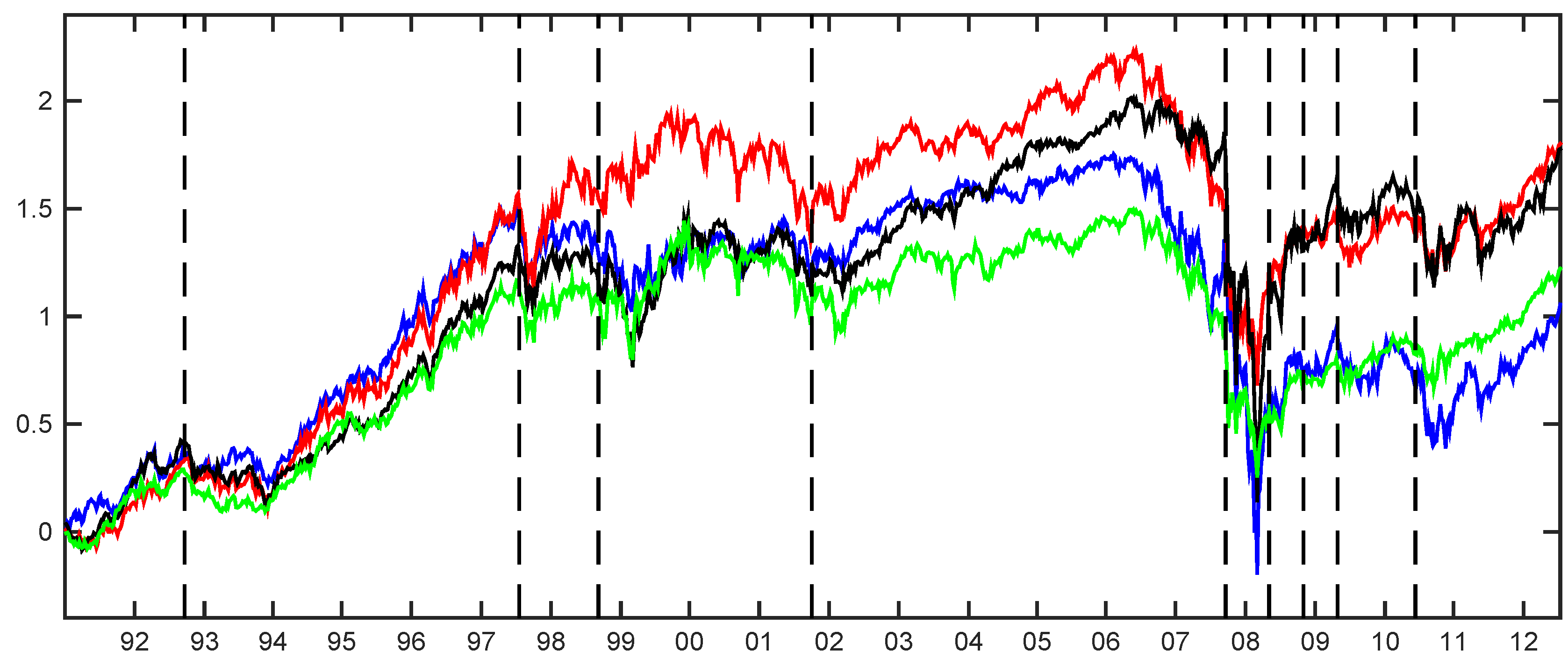
Figure 1. Cumulative returns of the different sectors: banks (blue line), financial services (red line), life insurance (dark line) and non-life insurance (green line). Vertical dotted lines represent major financial downturns: see Figure 1 for a detailed description.

Figure 1. Cumulative returns of the different sectors: banks (blue line), financial services (red line), life insurance (dark line) and non-life insurance (green line). Vertical dotted lines represent major financial downturns: see Figure 1 for a detailed description.

Figure 1 shows the time series of cumulative returns for all of the considered assets, from 2 January 1992, till the end of the sample. Vertical dotted lines refer to the following events: “Black Wednesday” (16 September 1992), the Asian crisis (July 1997), the Russian crisis (August 1998), the 11 September 2001, shock, the onset of the mortgage subprime crisis identified by the Bear Stearns hedge funds collapse (5 August 2007), the acquisition of Bear Stearns by JP Morgan Chase (16 March 2008), the collapse of Lehman brothers (15 September 2008), the peak of the onset of the recent GFC (9 March 2009) and the European sovereign-debt crisis of April 2010 (23 April 2010, Greek crisis). The figure gives insights about how the crisis periods affect the different sectors here considered. After the 2001 Twin Towers attack till the middle of 2007, the U.S. financial system experienced a long period of small perturbations and stability which ended shortly after the collapse of two Bear Stearns hedge funds in early August 2007. Starting from August 2007, the financial market experienced a drastic fall, as the subprime mortgage crisis led to a financial crisis and subsequent recession beginning in 2008. Several major financial institutions collapsed in September 2008, with significant disruption in the flow of credit to businesses and consumers and the onset of a severe global recession. The system hit bottom in March 2009, and then started a slow recovery, which culminated just before the European sovereign-debt crisis of April 2010. It is interesting to note that since the beginning of the 2007 global crisis all of the considered sectors experienced huge capital losses, with the banking sector (blue line) being the worst affected by the crisis. Moreover, banks and non-life insurance, on the one hand, and financial services and life insurance, on the other hand, have become more related after the European sovereign-debt crisis, displaying similar trends.

4.2. Estimation Results

In this section, we proceed by fitting the best model for the data considered and by estimating all of the parameters involved. To select the best model in the multivariate Student-t MS setting, we need to choose the number L of latent states. According to the current literature (see, e.g., Cappé et al. [28]; Rydén, [36]), we apply the Akaike information ceriterion (AIC) and the Bayesian information criterion (BIC), which involve different penalization terms depending on the number of non-redundant parameters. In particular, we fit the proposed model with a number of hidden states L from two to six. The results of this preliminary analysis are reported in Table 2, where it is evident that both information criteria prefer the model with four hidden states.

Table 2. Log-likelihood values, Akaike (AIC) and Schwarz (BIC) information criteria of the proposed Student-t MS model with different number of components. Bold face indicates the selected model.

L	Log-Likelihood	AIC	BIC
2	11,889.544	−23,713.088	−23,410.697
3	11,713.089	−23,320.177	−23,053.355
4	11,969.138	−23,788.276	−23,546.954
5	11,946.912	−23,695.824	−23,197.420
6	11,973.013	−23,696.025	−23,066.727

Table 2. Log-likelihood values, Akaike (AIC) and Schwarz (BIC) information criteria of the proposed Student-t MS model with different number of components. Bold face indicates the selected model.

L	Log-Likelihood	AIC	BIC
2	11,889.544	−23,713.088	−23,410.697
3	11,713.089	−23,320.177	−23,053.355
4	11,969.138	−23,788.276	−23,546.954
5	11,946.912	−23,695.824	−23,197.420
6	11,973.013	−23,696.025	−23,066.727

Table 3. Maximum likelihood parameter estimates of the selected Student-t MS model with four components. µ_l, for $l=1,2,\cdots ,L$, denote the location parameters, while the diagonal matrices Λ_l and the full matrices Ω_l for $l=1,2,\cdots ,L$ are such that ${\sum }_l={\mathsf{\Lambda }}_l{\mathsf{\Omega }}_l{\mathsf{\Lambda }}_l$, where ${\sum }_l$ is the scale matrix of the Student-t distribution.

µ $\times {\mathbf{10}}^{\mathbf{3}}$	Banks	Fin. Srvs	Life Insur.	Non-life Insur.
State 1	−6.8905	−0.2288	−8.1268	−2.7188
State 2	−4.5542	−4.2744	−1.9875	−3.4971
State 3	1.0459	1.8574	1.2758	1.9089
State 4	3.5818	4.4010	4.3724	2.9295
$\Lambda \times {\mathbf{10}}^{\mathbf{3}}$	Banks	Fin. Srvs	Life Insur.	Non-life Insur.
State 1	13.8891	7.0203	15.6855	4.3998
State 1	1.4302	1.6766	1.0333	1.0232
State 1	0.9998	0.6871	1.2204	0.3585
State 1	0.3427	0.5197	0.2827	0.3137
${\Omega }_1$	Banks	Fin. Srvs	Life Insur.	Non-life Insur.
Banks	1.0000
Fin. srvs	0.8399	1.0000
Life insur.	0.8511	0.8248	1.0000
Non-life insur.	0.6966	0.8013	0.8015	1.0000
${\Omega }_2$	Banks	Fin. Srvs	Life Insur.	Non-life Insur.
Banks	1.0000
Fin. srvs	0.8573	1.0000
Life insur.	0.7654	0.7771	1.0000
Non-life insur.	0.7683	0.7881	0.8205	1.0000
${\Omega }_3$	Banks	Fin. Srvs	Life Insur.	Non-life Insur.
Banks	1.0000
Fin. srvs	0.8807	1.0000
Life insur.	0.8537	0.8939	1.0000
Non-life insur.	0.7827	0.8472	0.8555	1.0000
${\Omega }_4$	Banks	Fin. Srvs	Life Insur.	Non-life Insur.
Banks	1.0000
Fin. srvs	0.8620	1.0000
Life insur.	0.7337	0.7678	1.0000
Non-life insur.	0.7250	0.7622	0.7792	1.0000

Table 3. Maximum likelihood parameter estimates of the selected Student-t MS model with four components. µ_l, for $l=1,2,\cdots ,L$, denote the location parameters, while the diagonal matrices Λ_l and the full matrices Ω_l for $l=1,2,\cdots ,L$ are such that ${\sum }_l={\mathsf{\Lambda }}_l{\mathsf{\Omega }}_l{\mathsf{\Lambda }}_l$, where ${\sum }_l$ is the scale matrix of the Student-t distribution.

µ $\times {\mathbf{10}}^{\mathbf{3}}$	Banks	Fin. Srvs	Life Insur.	Non-life Insur.
State 1	−6.8905	−0.2288	−8.1268	−2.7188
State 2	−4.5542	−4.2744	−1.9875	−3.4971
State 3	1.0459	1.8574	1.2758	1.9089
State 4	3.5818	4.4010	4.3724	2.9295
$\Lambda \times {\mathbf{10}}^{\mathbf{3}}$	Banks	Fin. Srvs	Life Insur.	Non-life Insur.
State 1	13.8891	7.0203	15.6855	4.3998
State 1	1.4302	1.6766	1.0333	1.0232
State 1	0.9998	0.6871	1.2204	0.3585
State 1	0.3427	0.5197	0.2827	0.3137
${\Omega }_1$	Banks	Fin. Srvs	Life Insur.	Non-life Insur.
Banks	1.0000
Fin. srvs	0.8399	1.0000
Life insur.	0.8511	0.8248	1.0000
Non-life insur.	0.6966	0.8013	0.8015	1.0000
${\Omega }_2$	Banks	Fin. Srvs	Life Insur.	Non-life Insur.
Banks	1.0000
Fin. srvs	0.8573	1.0000
Life insur.	0.7654	0.7771	1.0000
Non-life insur.	0.7683	0.7881	0.8205	1.0000
${\Omega }_3$	Banks	Fin. Srvs	Life Insur.	Non-life Insur.
Banks	1.0000
Fin. srvs	0.8807	1.0000
Life insur.	0.8537	0.8939	1.0000
Non-life insur.	0.7827	0.8472	0.8555	1.0000
${\Omega }_4$	Banks	Fin. Srvs	Life Insur.	Non-life Insur.
Banks	1.0000
Fin. srvs	0.8620	1.0000
Life insur.	0.7337	0.7678	1.0000
Non-life insur.	0.7250	0.7622	0.7792	1.0000

Table 4. Maximum likelihood estimates of the degrees of freedom ν, the initial probability δ and the transition probability matrix $\mathbf{\text{Q}}$ of the Markov chain for the selected Student-t MS model with four components.

ν	State 1	State 2	State 3	State 4
	15.6839	10.2542	11.0300	9.9473
δ	State 1	State 2	State 3	State 4
	0.0000	1.0000	0.0000	0.0000
$\mathbf{\text{Q}}$	State 1	State 2	State 3	State 4
State 1	0.8934	0.1066	0.0000	0.0000
State 2	0.0244	0.9608	0.0071	0.0077
State 3	0.0000	0.0000	0.9919	0.0081
State 4	0.0000	0.0052	0.0022	0.9926

Table 4. Maximum likelihood estimates of the degrees of freedom ν, the initial probability δ and the transition probability matrix $\mathbf{\text{Q}}$ of the Markov chain for the selected Student-t MS model with four components.

ν	State 1	State 2	State 3	State 4
	15.6839	10.2542	11.0300	9.9473
δ	State 1	State 2	State 3	State 4
	0.0000	1.0000	0.0000	0.0000
$\mathbf{\text{Q}}$	State 1	State 2	State 3	State 4
State 1	0.8934	0.1066	0.0000	0.0000
State 2	0.0244	0.9608	0.0071	0.0077
State 3	0.0000	0.0000	0.9919	0.0081
State 4	0.0000	0.0052	0.0022	0.9926

For the selected model, Table 3 and Table 4 summarize parameter estimates. The dynamical evolution of risk-return profiles, often documented in the financial literature, is captured well by our model. In fact, we observe in Table 3 that two positive regimes (States 3 and 4) and two negative regimes (States 1 and 2) are identified according to significantly different state-specific return means. Furthermore, large negative returns (State 1) are characterized by quite large standard deviations (parameter Λ), as opposed to negative returns, where standard deviations are substantially lower. States 2 and 3 identify periods of low volatility associated with moderately negative and positive mean returns, respectively. This essentially implies that States 1 and 4 can be identified as periods of financial turbulence and stability, while States 2 and 3 are regimes where the financial system transits just before or immediately after a crisis period. 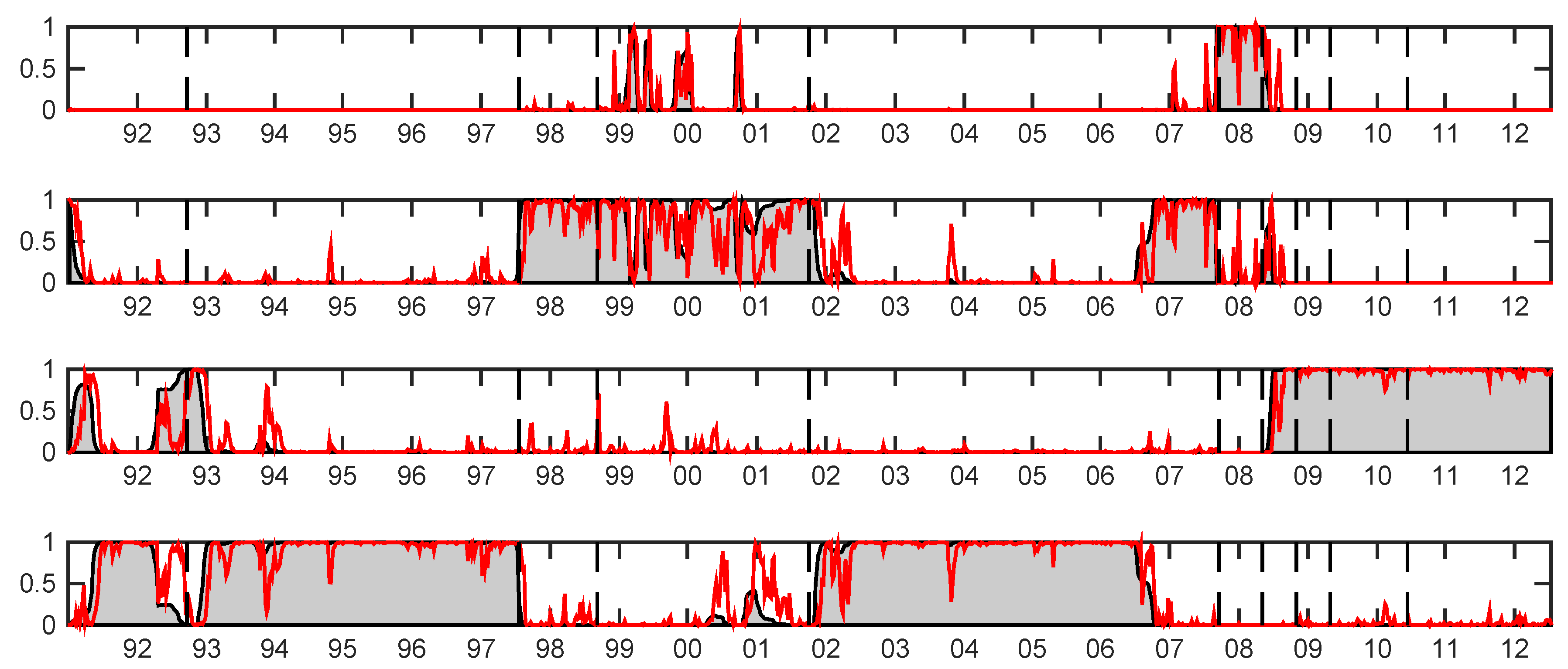This latter observation can be evinced also by inspecting Figure 2 displaying the Markovian predicted and smoothed probabilities of being in a given state at each time period, denoted by $\mathbb{P}\left(S_t\mid {\mathcal{I}}_T\right)$. During the 2007–2008 GFC, for example, we observe that the predictive probability (red line) of being in State 1 (turbulence) is larger than 99%. During the period immediately before the 2007 crisis, covering most of the 2006 and 2007 years, till the collapse of the Bear Stearns hedge fund in August 2007, the system visits the transitory State 2, which corresponds to the pre-crisis regime. The same empirical findings are confirmed by inspecting the smoothed probabilities; the grey area in Figure 3. All of those results document the importance of choosing the right model specification in order to understand the global dynamics of the economic system.

As extensively documented in Bernardi et al. [21], the multivariate Student-t approach considered here is also able to identify different co-movement effects among stocks, measured by the state-specific correlations (parameter Ω). As expected, correlations are higher during crisis periods, while during more stable phases, variances are relatively low and the contagion effect is less marked.

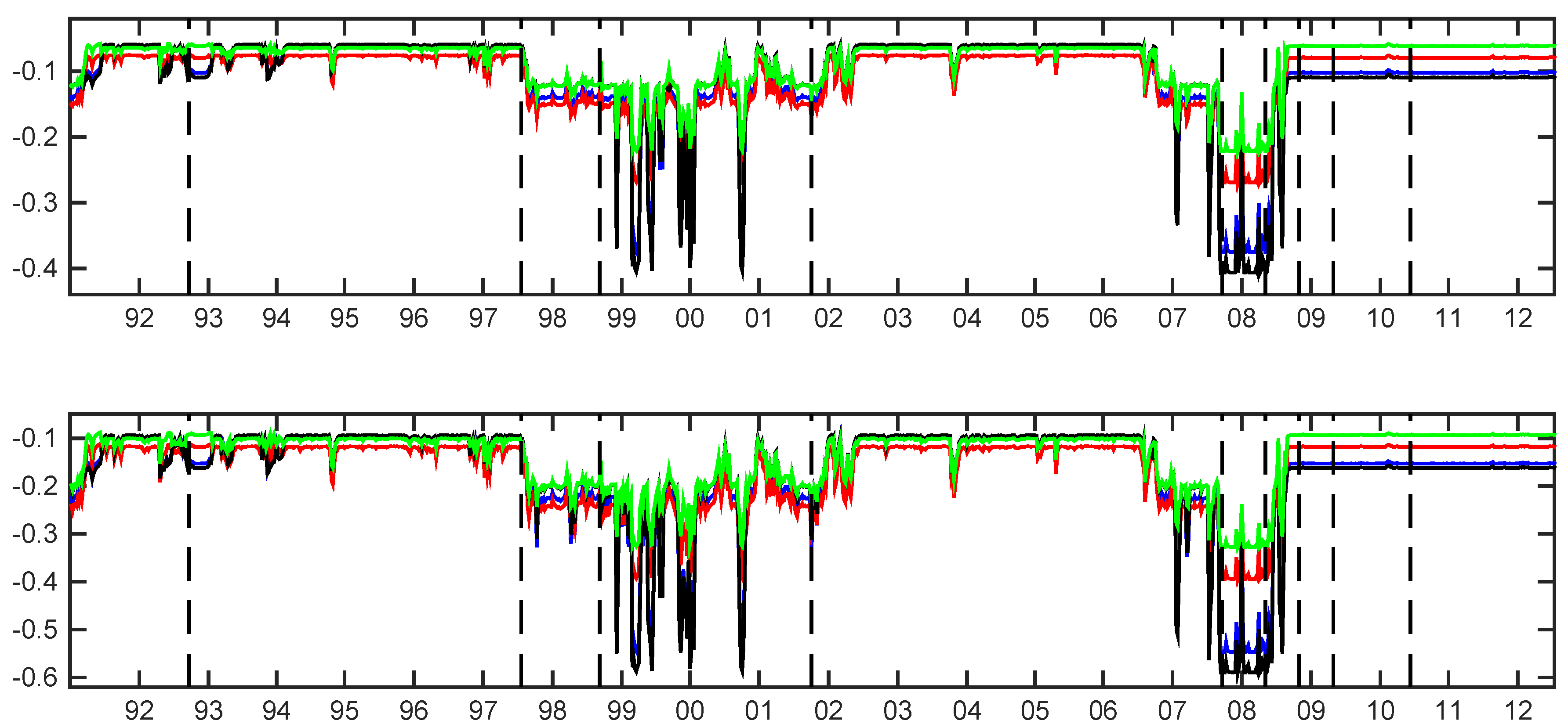
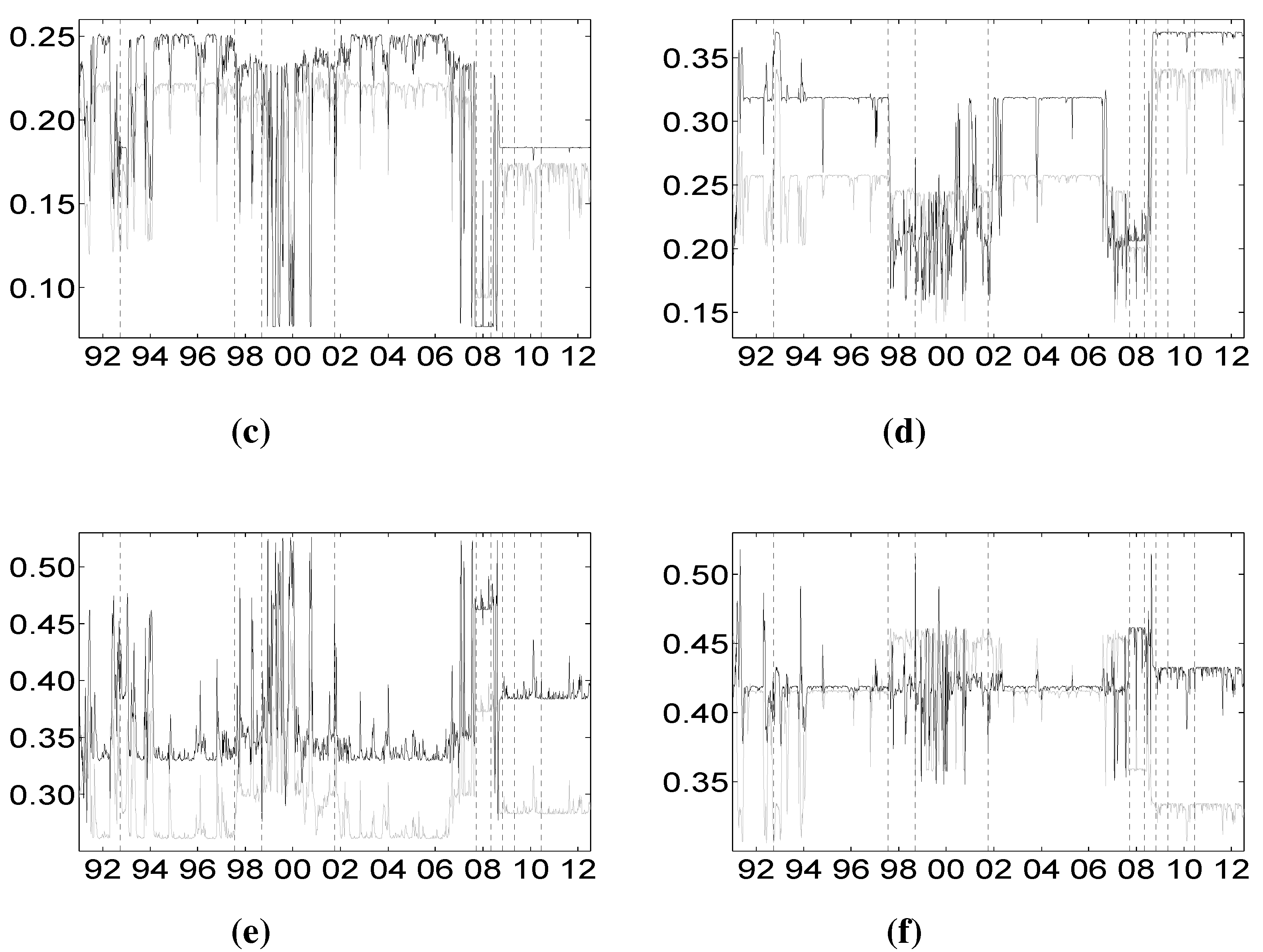
Figure 2. Total risk evaluated by multiple-conditional value-at-risk (CoVaR) (top) and multiple-conditional expected shortfall (CoES) (bottom) for the different sectors: banks (blue line), financial services (red line), life insurance (dark line) and non-life insurance (green line). Vertical dotted lines represent major financial downturns: see Figure 1 for a detailed description.

Figure 2. Total risk evaluated by multiple-conditional value-at-risk (CoVaR) (top) and multiple-conditional expected shortfall (CoES) (bottom) for the different sectors: banks (blue line), financial services (red line), life insurance (dark line) and non-life insurance (green line). Vertical dotted lines represent major financial downturns: see Figure 1 for a detailed description.

Figure 3. Smoothed probabilities of visiting the states of the Markovian chain $\mathbb{P}\left(S_t=j\mid {\mathcal{I}}_T\right)$ for $j=1,\cdots ,4$ and $t=1,2,\cdots ,T$ (from top to bottom) implied by the Student-t model with four components. The superimposed red lines represent the predictive probabilities $\mathbb{P}\left(S_t=j\mid {\mathcal{I}}_{t-1}\right)$ for $j=1,\cdots ,4$ and $t=1,2,\cdots ,T$. States 1 and 4 are identified as periods of financial turbulence and stability, respectively, while States 2 and 3 are regimes where the financial system transits just before or immediately after a crisis period. Vertical dotted lines represent major financial downturns: see Figure 1 for a detailed description.

Figure 3. Smoothed probabilities of visiting the states of the Markovian chain $\mathbb{P}\left(S_t=j\mid {\mathcal{I}}_T\right)$ for $j=1,\cdots ,4$ and $t=1,2,\cdots ,T$ (from top to bottom) implied by the Student-t model with four components. The superimposed red lines represent the predictive probabilities $\mathbb{P}\left(S_t=j\mid {\mathcal{I}}_{t-1}\right)$ for $j=1,\cdots ,4$ and $t=1,2,\cdots ,T$. States 1 and 4 are identified as periods of financial turbulence and stability, respectively, while States 2 and 3 are regimes where the financial system transits just before or immediately after a crisis period. Vertical dotted lines represent major financial downturns: see Figure 1 for a detailed description.

Table 4 provides parameter estimates of the Student-t degrees-of-freedom ν and the transition probabilities Q of the hidden Markov chain. Looking at the ν parameters’ estimate, fat-tails have been detected, and this is in line with empirically-observed stylized facts. Moreover, the introduction of conditional Student-t distributions increases the state persistence significantly, resulting in longer and more stable volatility periods. This is confirmed by the transition matrix estimate. The large off-diagonal transition probabilities in all states, except the first one, confirm the large persistence of the transitory states (2 and 3), as well as State 4 of financial stability. On the contrary, State 1 of financial crisis is characterized by a smaller probability value on the main diagonal, denoting a small level of persistence of the crisis periods. The crisis state is also characterized by a moderately large probability to move to State 2, suggesting that after coming out from a crisis, the system enters a period of “moderate” financial turbulence.

It is important to note that, although parameter estimates provide relevant information to support the policy decision-making process, they do not provide enough insights to evaluate extreme tail interdependence.

4.3. Risk Contributions

The goal of this section is to analyze how the total risk is shared among different sectors by inspecting the time evolution of the Shapley values risk measures introduced in the previous sections.

We examine whether the extreme-tail interdependence among banks, financial services and insurance sectors has changed over time. The interconnectedness among sectors, and, in particular, between the financial and the insurance sectors, have been highly investigated in the recent literature. In their empirical investigation, Bernal et al. [10], for example, found that banks contribute relatively the most to systemic risk in the Eurozone, while the insurance industry is the most systemically risky sector in the U.S. for the period 2004–2012. Recently, Chen et al. [12] and Billio et al. [6], using univariate Granger-causality analyses, show a significant two-way interconnection between banking and insurance sectors. Our model-based approach instead is able to investigate the tail risk contribution of each sector to the risk of all of the remaining ones in a multivariate framework. Furthermore, our analysis considers different distress events jointly affecting the market participants health level.

In Figure 2, we plot the dynamic evolution of the total risk of each sector. By total risk, we mean the risk of the sector when all of the remaining sectors are in distress. This figure provides the benchmark for authorities to calculate individual sector’s risk contributions. The dynamic evolution of the total risk for all sectors suggests that, during the analyzed period, there have been four major downside peaks: the Russian crisis at the end 1998, which partially overlaps the dot-com bubble of 1999–2000; the September 11 shock; and the recent GFC of 2007–2009. Interestingly, both the Russian crisis and the recent mortgage subprime crisis of 2007, which are followed by several years of financial turbulence affecting all of the sectors, are anticipated by a long period where the total risk increased significantly. Although both crisis episodes have been characterized by different durations, as well as financial and economic conditions, we observe that they are anticipated by an increased level of overall risk. This evidence supports the use of the total risk measure as a leading indicator for the financial crisis. Concerning in particular the Russian crisis, a careful inspection of Figure 2 reveals that the total risk for all sectors increased suddenly in conjunction with the antecedent Asian crisis of middle 1997. Then, the system experienced a long period of financial instability encompassing all of the three subsequent crises culminating with the Twin towers attack of September, 2001. Concerning the recent global crisis, instead, we observe that the total risk increases a long time before the Bear Stearns hedge found collapse of August, 2007, for all sectors. In fact, looking at the predicted and smoothed probabilities depicted in Figure 2, we note that the system transits into State 2 since mid-2006, anticipating the subsequent market turbulence. It is evident from Figure 2 that the predicted and smoothed probabilities provide the same signal about the underlying state that the financial system is experiencing. Another important difference between the two periods of financial crisis, 1997–2001 and 2007–2009, emerges by comparing the total risk evolution with the predicted and smoothed probabilities plotted in Figure 2 and Figure 3, respectively. It is evident that the latter financial crisis has been more persistent than those occurring in the previous decades. In fact, during the period 1997–2001, the system is in State 2 of moderate instability, while during the period 2007–2009, the system is in State 1 of financial turbulence for most of the time. Finally, we observed that the U.S. market is not affected by the European sovereign debt crisis in May 2010.

It is interesting to note that the total risk dynamics in Figure 2 suggests that, before the 2007, the financial services sector (red line) is the most affected by the other sectors’ distress, while the banking and the insurance sectors display a similar low level of risk, whereupon this ordering completely change by the beginning of 2009, with banks (blue line) and life insurance (dark line) being the most risky sectors. In fact, we observe that the total risk contributions change during crisis periods, becoming larger in level and reversing the ordering of importance.

As said before, the total risk contribution analysis identifies the sector most affected by the crisis of all of the remaining ones during different periods of time, providing an important tool for risk management. This analysis by itself is not conclusive, because it considers all of the other sectors, except one, at their distress level. This is the reason why, once we get the ${\Delta }^{\mathsf{M}}$CoVaR and ${\Delta }^{\mathsf{M}}$CoES risk measures for each sector given all the possible combinations of the remaining sectors’ distress events, we apply the Shapley value methodology to compose the puzzle of their synthesis to provide a unifying measure. The resulting Shapley values act as an overall risk distributor among the market participants, providing the marginal contributions to each of the considered sectors of the remaining sectors’ distress. In our case, since we are measuring interdependencies among four sectors, we have three Shapley value contributions for each of them. 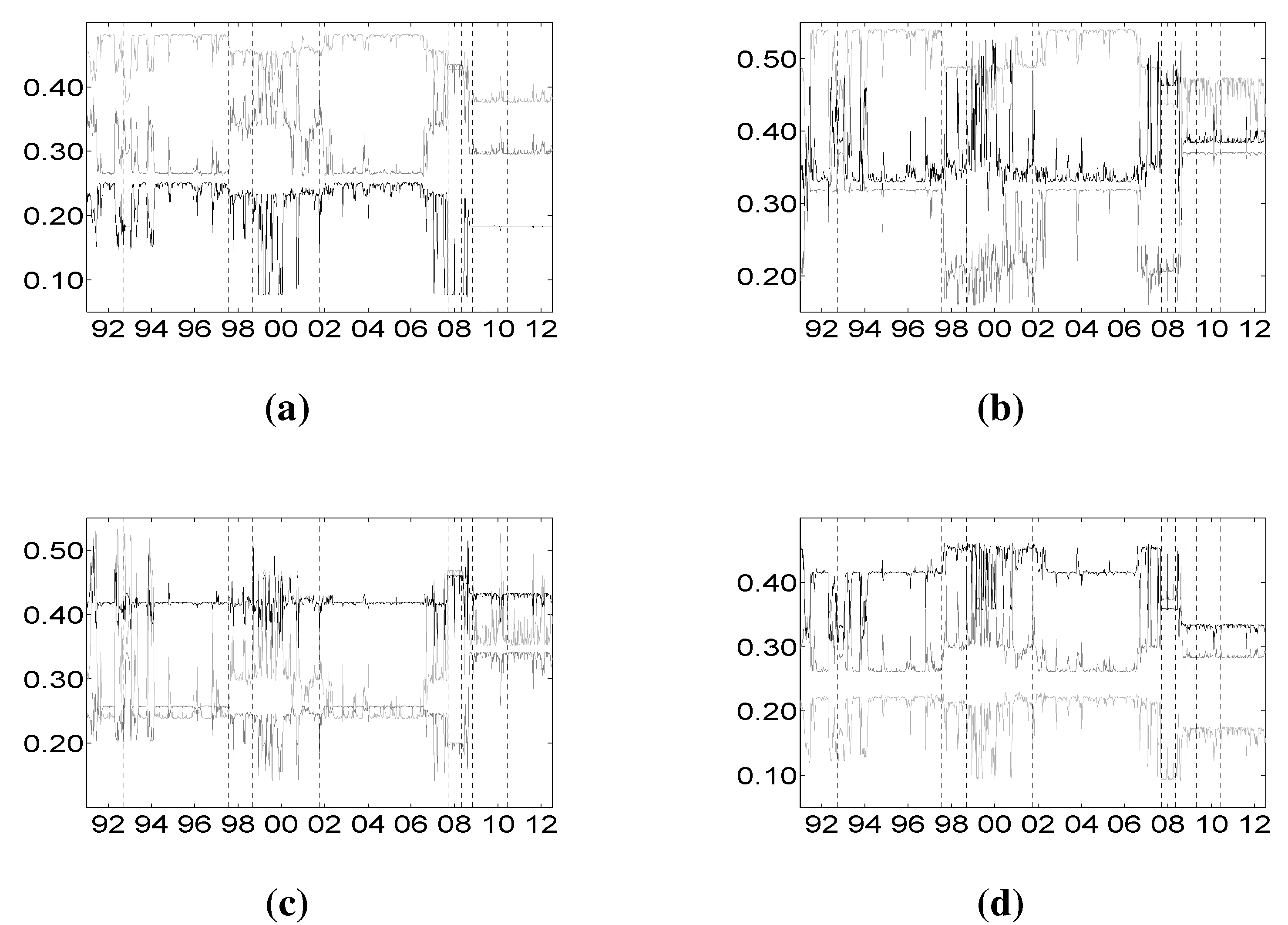Figure 4 and Figure 5 plot the individual marginal contributions calculated by means of the Shapley value ${\mathrm{ShV}}_i$ based on ${\Delta }^{\mathsf{M}}{\mathrm{CoVaR}}_{i|{\mathcal{J}}_{\mathsf{D}}}$ and ${\Delta }^{\mathsf{M}}{\mathrm{CoES}}_{i|{\mathcal{J}}_{\mathsf{D}}}$, respectively. 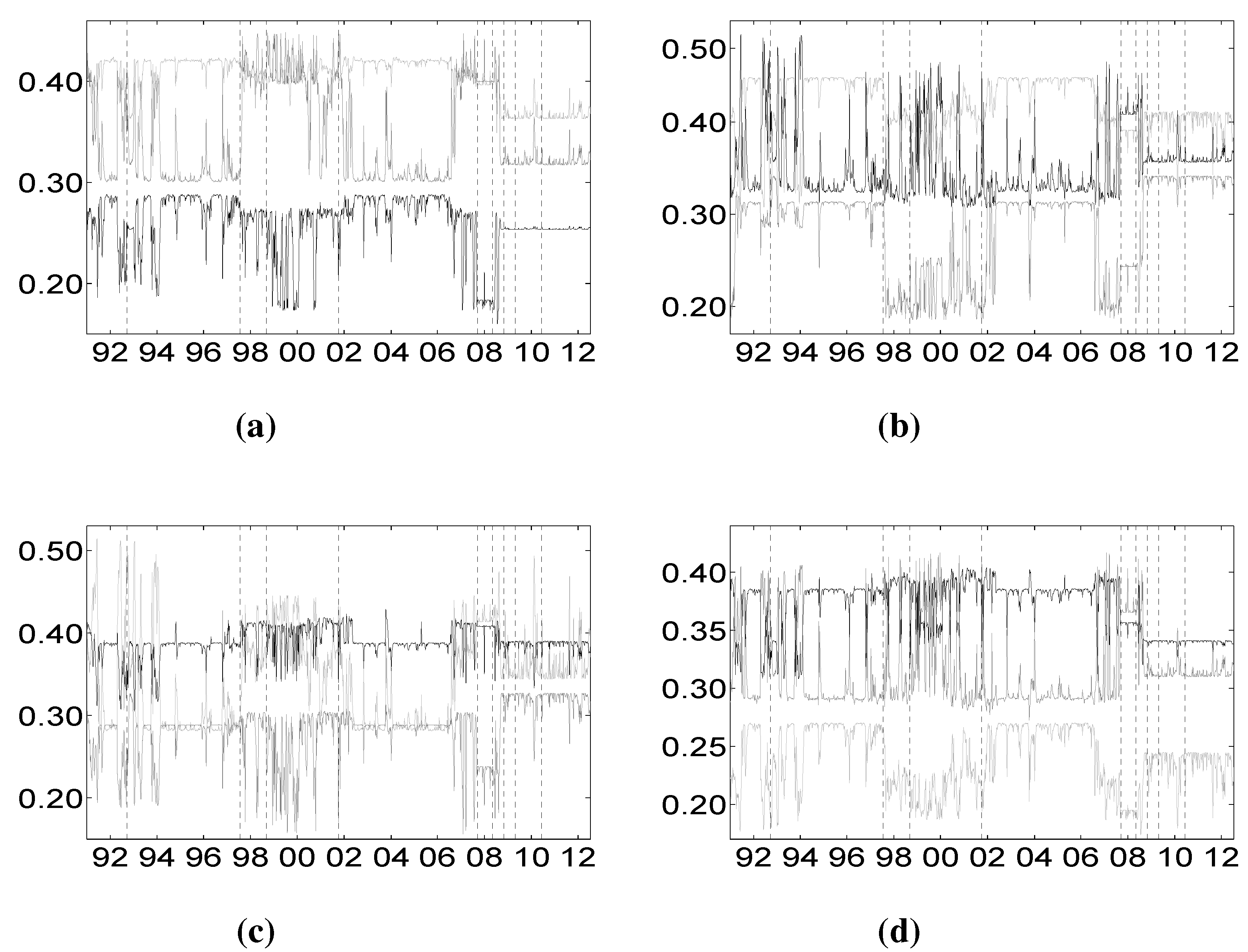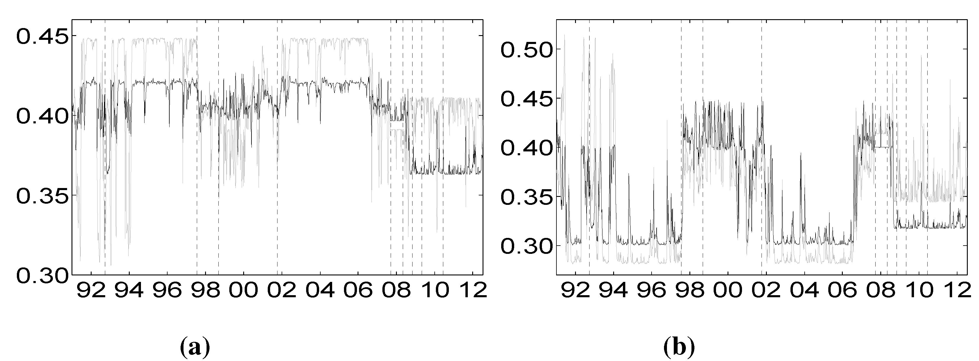Figure 4a plots the Shapley value contributions of financial services, life insurance and non-life insurance on the banking sector. We observe that the financial services sector contributes more to the distress of the banking sector than both the life and non-life insurance sectors, independent of the overall financial situation identified by the hidden state. Furthermore, during periods of financial stability, the contribution of financial services is about two-times larger than that of life and non-life insurance. During periods of crisis, instead, the contributions of financial services and non-life insurance decrease, while that of life insurance increases, so that the contribution of non-life insurance becomes negligible and those of financial services and life insurance approach almost the same level. Figure 4b plots the contributions on the financial services sector. The picture is similar to the one in Figure 4a, with the role of banks and financial services and that of life and non-life insurance reversed. This essentially means that banks and financial services are strongly interdependent. Figure 4c and Figure 4d plot the contributions of the life and non-life insurance sectors, respectively. Comparing the two figures, we observe that these sectors are highly interdependent during the period of crisis, as well as during the period of financial stability. In Figure 4c, the contributions of banks and financial services to life insurance looks the same, and they increase suddenly after the recent GFC ends. In Figure 4d the contribution of banks to non-life insurance is low compared to other sectors’ contributions, suggesting that the banking sector is more connected with life insurance (see Figure 4c) than with the non-life one. The results here presented are confirmed by inspecting Figure 5, where individual marginal contributions are calculated by means of the Shapley value ${\mathrm{ShV}}_i$ based on ${\Delta }^{\mathsf{M}}{\mathrm{CoES}}_{i|{\mathcal{J}}_{\mathsf{D}}}$.

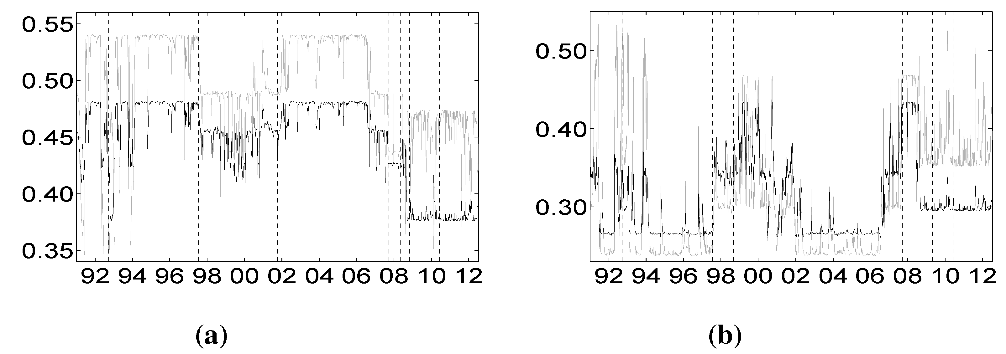
To deeply understand the relative impact of each sector’s financial distress on all of the other sectors, we plot the two-way comparisons of marginal contributions for all of the possible pairs of sectors. Figure 6 and Figure 7 plot the comparisons vis-à-vis based on the Shapley value ${\Delta }^{\mathsf{M}}$CoVaR and ${\Delta }^{\mathsf{M}}$CoES, respectively. Figure 6a and Figure 7a consider the banking and diversified financial services sectors. Independent of the hidden state, it is clear that the financial services’ distress impacts more the banking sector than the other way around. Figure 6b and Figure 7b consider the banking sector against the life insurance one. This picture highlights an important aspect of the extreme interdependence between these sectors that can be captured by the dynamic Shapley approach here proposed. In particular, it is evident that, prior to the recent GFC of 2007–2009, banks impact more the life insurance during periods of financial stability (for example, 2002–2006), than vice versa, while, after the end of 2008, the order of importance between these two sectors is reversed. This behavior is peculiar of the banking and life insurance sectors and does not characterize the relationship between the banking sector on non-life insurance depicted in Figure 6c and Figure 7c. These two latter sectors seem to be highly interdependent with a slight predominance of the banks. Figure 6b and Figure 6c consider the impact of the financial sector on life and non-life insurance sectors, providing clear evidence that the financial sector highly impacts the insurance sector. Prior to the 2008 GFC, the impact of the financial services sector distress on that of life insurance is higher during stable periods than during turbulent periods, while after the end of the 2008 crisis, the financial services sector and the life insurance sector become more interconnected. Finally, Figure 6f and Figure 7f consider the interdependence between the insurance sectors, providing clear evidence that these two sectors are highly connected till the end of 2008. After the end of 2008, the relative weight of life insurance decreased.

Figure 4. Shalpey value ${\Delta }^{\mathsf{M}}$-CoVaR of the different sectors against banks (a), financial services (b), life insurance (c) and non-life insurance (d). Vertical dotted lines represent major financial downturns: see Figure 1 for a detailed description. (a) Financial services (light gray), life (gray) and non-life (dark) insurance against banks; (b) banks (light gray), life (gray) and non-life (dark) insurance against financial services; (c) banks (light gray), financial services (gray) and non-life insurance (dark) against the life insurance index; (d) banks (light gray), financial services (gray) and life insurance (dark) against the non-life insurance index.

Figure 4. Shalpey value ${\Delta }^{\mathsf{M}}$-CoVaR of the different sectors against banks (a), financial services (b), life insurance (c) and non-life insurance (d). Vertical dotted lines represent major financial downturns: see Figure 1 for a detailed description. (a) Financial services (light gray), life (gray) and non-life (dark) insurance against banks; (b) banks (light gray), life (gray) and non-life (dark) insurance against financial services; (c) banks (light gray), financial services (gray) and non-life insurance (dark) against the life insurance index; (d) banks (light gray), financial services (gray) and life insurance (dark) against the non-life insurance index.

Table 5 compares the proposed Shapley-${\Delta }^{\mathsf{M}}$CoVaR method with the standard ΔCoVaR approach of Adrian and Brunnermeier [14], for each of the considered sectors against each other. For each pair of sectors, the standard ΔCoVaR risk measure is calculated by firstly estimating the Student-t MS model on the corresponding time series of bivariate returns. The ΔCoVaR measure is then calculated by applying Equation (6), where the set of distress sectors ${\mathcal{J}}_{\mathsf{D}}$ consist of only one element, while the set of sectors at the normal state ${\mathcal{J}}_{\mathsf{N}}$ is empty. Is is evident that, as expected, except for the banks and life insurance pairs, the signal provided by the standard ΔCoVaR differs significantly from that provided by our risk measure based on the Shapley value. As discussed by Bernardi et al. [21], the two risk measures may coincide only under the conditional independence assumption for the set of conditioning events. Moreover, the discrepancy between the Shapley value ${\Delta }^{\mathsf{M}}$CoVaR and the standard ΔCoVaR of Adrian and Brunnermeier [14] further justifies the provided “multiple” analysis. Accounting for multiple joint distress events helps to reveal the underlying structure of the tail risk interdependence among sectors that would probably remain otherwise shadowed.

Figure 5. Shalpey value ${\Delta }^{\mathsf{M}}$-CoES of the different sectors against banks (a), financial services (b), life insurance (c) and non-life insurance (d). Vertical dotted lines represent major financial downturns: see Figure 1 for a detailed description. (a) Financial services (light gray), life (gray) and non-life (dark) insurance against banks; (b) banks (light gray), life (gray) and non-life (dark) insurance against financial services; (c) banks (light gray), financial services (gray) and non-life insurance (dark) against the life insurance index; (d) banks (light gray), financial services (gray) and life insurance (dark) against the non-life insurance index.

Figure 5. Shalpey value ${\Delta }^{\mathsf{M}}$-CoES of the different sectors against banks (a), financial services (b), life insurance (c) and non-life insurance (d). Vertical dotted lines represent major financial downturns: see Figure 1 for a detailed description. (a) Financial services (light gray), life (gray) and non-life (dark) insurance against banks; (b) banks (light gray), life (gray) and non-life (dark) insurance against financial services; (c) banks (light gray), financial services (gray) and non-life insurance (dark) against the life insurance index; (d) banks (light gray), financial services (gray) and life insurance (dark) against the non-life insurance index.

Figure 6. Comparisons of Shapley values ${\Delta }^{\mathsf{M}}$CoVaR for the different sectors. Vertical dotted lines represent major financial downturns: see Figure 1 for a detailed description. (a) Distress of banks on financial services (dark) and vice versa (light gray); (b) distress of banks on life insurance (dark) and vice versa (light gray); (c) distress of banks on non-life insurance (dark) and vice versa (light gray); (d) distress of financial srvs on life insurance (dark) and vice versa (light gray); (e) distress of financial servis on non-life insurance (dark) and vice versa (light gray); (f) distress of life insurance on non-life insurance (dark) and vice versa (light gray).

Figure 6. Comparisons of Shapley values ${\Delta }^{\mathsf{M}}$CoVaR for the different sectors. Vertical dotted lines represent major financial downturns: see Figure 1 for a detailed description. (a) Distress of banks on financial services (dark) and vice versa (light gray); (b) distress of banks on life insurance (dark) and vice versa (light gray); (c) distress of banks on non-life insurance (dark) and vice versa (light gray); (d) distress of financial srvs on life insurance (dark) and vice versa (light gray); (e) distress of financial servis on non-life insurance (dark) and vice versa (light gray); (f) distress of life insurance on non-life insurance (dark) and vice versa (light gray).

Figure 7. Comparisons of Shapley values ${\Delta }^{\mathsf{M}}$CoES for the different sectors. Vertical dotted lines represent major financial downturns: see Figure 1 for a detailed description. (a) Distress of banks on financial services (dark) and vice versa (light gray); (b) distress of banks on life insurance (dark) and vice versa (light gray); (c) distress of banks on non-life insurance (dark) and vice versa (light gray); (d) distress of financial services on life insurance (dark) and vice versa (light gray); (e) distress of financial services on non-life insurance (dark) and vice versa (light gray); (f) distress of life insurance on non-life insurance (dark) and vice versa (light gray).

Figure 7. Comparisons of Shapley values ${\Delta }^{\mathsf{M}}$CoES for the different sectors. Vertical dotted lines represent major financial downturns: see Figure 1 for a detailed description. (a) Distress of banks on financial services (dark) and vice versa (light gray); (b) distress of banks on life insurance (dark) and vice versa (light gray); (c) distress of banks on non-life insurance (dark) and vice versa (light gray); (d) distress of financial services on life insurance (dark) and vice versa (light gray); (e) distress of financial services on non-life insurance (dark) and vice versa (light gray); (f) distress of life insurance on non-life insurance (dark) and vice versa (light gray).

Table 5. Comparison of the Shapley value ${\Delta }^{\mathsf{M}}$CoVaR (light gray) and the Adrian and Brunnermeier’s standard ΔCoVaR approach (light gray) for all of the sectors against each other. Vertical dotted lines represent major financial downturns: see Figure 1 for a detailed description.

	Banks	Fin. Srvs	Life Ins.	non-life Ins.
Banks
Fin. Srvs
Life Ins.
non-life Ins.

Table 5. Comparison of the Shapley value ${\Delta }^{\mathsf{M}}$CoVaR (light gray) and the Adrian and Brunnermeier’s standard ΔCoVaR approach (light gray) for all of the sectors against each other. Vertical dotted lines represent major financial downturns: see Figure 1 for a detailed description.

	Banks	Fin. Srvs	Life Ins.	non-life Ins.
Banks
Fin. Srvs
Life Ins.
non-life Ins.

5. Discussion

The model-based approach to the overall risk assessment developed in Bernardi et al. [21] and applied here to four sectors belonging to the U.S. Dow Jones Composite Index allows one to understand the dynamic evolution of the tail risk interdependence among the banking, life and non-life insurance and other financial services sectors. Our empirical findings suggest that each financial sector significantly impacts the others during crisis periods, as well as during more stable phases. When comparing the contribution of each financial industry, banks appear to be the major source of risk for all of the remaining ones, followed by the financial services and the insurance sectors. These results are in line with previous findings (see, e.g., Bernal et al. [10]) and are supported by theoretical arguments. Adams et al. [7] and Girardi and Ergün [17], for example, found that the banking sector is systemically riskier than the insurance sector. Banks are particularly fragile institutions because of their core business, especially credit activity to households and corporate companies along with short-term funding, making the banking sector particularly exposed to the overall risk. Insurance companies, instead, generally fund themselves through long-term premiums and have higher disposable liquidity. This latter argument plays an important role, since financial crises usually begin with a liquidity squeeze that further weakens the capital position of vulnerable firms. Another argument is that balance sheets of banks are highly volatile and exposed to economic cycles, while insurance companies usually present simple and economically-stable balance sheets due to their long term-oriented business. Recently, the financial literature has pointed out the fact that banks are also much more interconnected than insurance companies through interbank lending, such as the repo market; see Gorton and Metrick [37]. Eventually, the size of the banking sector being much greater than the one of the insurance sector can also be a factor explaining that banks appear as the most risky in our study. Finally, our results regarding the systemic role of the four financial sectors in the United States are consistent with recent arguments raised in the literature emphasizing the risk associated with the fast growing, non-core activities (such as credit derivatives) of insurance companies (see, e.g., Bell and Keller [38]; Cummins and Weiss [1]). In fact, the non-core activities of U.S. insurance firms highly increased over the last decade.

6. Conclusions

This paper aims to assess the contribution of the different sectors of the financial system to the overall risk and to measure their degree of interdependence. To that end, we split the financial system into four sectors corresponding respectively to the banking, life and non-life insurance and other financial services industries. The impact of distress within any one of these sectors is measured using the Shapley value ${\Delta }^{\mathsf{M}}$CoVaR (or ${\Delta }^{\mathsf{M}}$CoES) risk measure proposed by Bernardi et al. [21]. More precisely, the Shapley value ${\Delta }^{\mathsf{M}}$CoVaR (${\Delta }^{\mathsf{M}}$CoES) extends the traditional ΔCoVaR approach of Adrian and Brunnermeier [14] to the case where multiple distress events are jointly observed, as is often the case during periods of financial instability. The Shapley value ${\Delta }^{\mathsf{M}}$CoVaR and ${\Delta }^{\mathsf{M}}$CoES can therefore be interpreted as the additional level of risk faced by each sector arising from the distress of one or more of the remaining financial sectors of interest. Empirical results reveal that in the U.S. financial market, for the period ranging from 1992 to 2012, the banking sector contributes relatively the most to the risk of all other sectors during periods of distress affecting this sector. By contrast, the life insurance industry is the least risky financial sector in the United States for the same period of time. Furthermore, life and non-life insurance industries appear to be highly interdependent, while diversified financial services seem to depend more on the banking system than the remaining sectors. This essentially means that during periods of financial instability, large losses in the banking sector affect the financial services sector more than the insurance sector. Finally, concerning the degree of interdependence between the insurance and banking sectors, our empirical findings suggest that insurers, as well as the other sectors may contribute to the spread of financial risk.