Asymmetric Realized Volatility Risk

Abstract

In this paper, we document that realized variation measures constructed from high-frequency returns reveal a large degree of volatility risk in stock and index returns, where we characterize volatility risk by the extent to which forecasting errors in realized volatility are substantive. Even though returns standardized by ex post quadratic variation measures are nearly Gaussian, this unpredictability brings considerably more uncertainty to the empirically relevant ex ante distribution of returns. Explicitly modeling this volatility risk is fundamental. We propose a dually asymmetric realized volatility model, which incorporates the fact that realized volatility series are systematically more volatile in high volatility periods. Returns in this framework display time varying volatility, skewness and kurtosis. We provide a detailed account of the empirical advantages of the model using data on the S&P 500 index and eight other indexes and stocks.

1. Introduction

This paper concerns the unpredictable time series component of realized volatility. We argue that a large and time varying realized volatility risk (defined as the time series volatility of realized volatility) is an essential stylized fact of index and stock returns that should be thoughtfully incorporated into econometric models of volatility. Our main contribution is twofold. First, we provide the empirical and theoretical motivation showing how the stochastic structure of the innovations in volatility have fundamental implications for applications of realized volatility models. Second, we go beyond extensions of standard realized volatility models to account for conditional heteroskedasticity (e.g., [1]) and bring to the forefront of our modeling approach the fact that realized volatility series exhibit a substantial degree of (time-varying) volatility themselves.

In a standard stochastic volatility setting where return innovations (conditional on the latent volatility) follow a Gaussian distribution, the degree of volatility risk is the key determinant of the excess kurtosis in the distribution of returns conditional on past information. Even though asset returns standardized by ex post quadratic variation measures are nearly Gaussian, returns standardized by fitted or predicted values of time series models of volatility are far from normal. Given the volatility in volatility, this is expected and should not be seen as evidence against those models; explicitly modeling the higher moments is necessary. If future realized volatility is difficult to predict, a focus on forecasting models will be insufficient for meaningfully modeling of the tails of the return distribution, which in many cases (e.g., risk management) is the main objective of the econometrician.

Our paper is a first step in trying to fully exploit the fact that the realized volatility framework allows not only for significant advances in the conditional volatility of asset returns, but also the higher moments and the longer-term distributions of price changes. Both strongly depend on volatility risk. The intuition for this argument is straightforward. When realized volatility is available, we do not have to rely only on rare realizations on return data to identify the tails of the return distribution: naturally, days of very high volatility are far more frequent than days of very high volatility and large return shocks. Likewise, a model with time-varying return kurtosis (an implication of time varying volatility risk), which would be very hard to identify from return data alone, can be easily estimated in a realized volatility framework.

In light of these arguments, we propose a new model for returns and realized volatility. The main new feature of this model is to explicitly account for the fact that realized volatility series are systematically more volatile in high volatility periods. While this finding has been suggested before in the options literature (see, for example, [2,3]), this relation has received little attention in the volatility literature. In the first paper to consider the volatility of realized volatility, Corsi et al. [1] extend the typical framework for modeling realized volatility by specifying a GARCH process to allow for clustering in the squared residuals of their realized volatility model. The same approach is followed by Bollerslev et al. [4]. In this paper we consider a parsimonious specification, where the variance of the realized volatility innovations is a linear function of the square of the volatility level, which we take to be the conditional mean of realized volatility. Another salient aspect of our model is the emphasis on extended leverage effects (following [5]). Because of the returns/volatility, volatility/volatility risk asymmetries, we call this framework the dually asymmetric realized volatility model.

Our empirical analysis uses high frequency data for the S&P 500 index and eight more series (between major stocks and indexes) from 1996 to 2009 to document the importance of volatility risk and to analyze the performance of the dually realized volatility model when compared to other standard alternatives. We show that our volatility risk specification consistently improves forecasting performance across these series and enhances the ability of the realized volatility model to account for large movements in volatility. Consistently with the central theme of this paper, however, the forecasting improvements brought by the best models are small in relation to the volatility of realized volatility. Our results for the volatility of realized volatility are stronger than the ones obtained by Corsi et al. [1] in that we can conclude that ignoring volatility risk has a severe adverse impact on point and density forecasting for realized volatility.

Other contributions to the realized volatility modeling and forecasting literature are exemplified by Andersen et al. [6], the HAR (heterogeneous autoregressive) model of Corsi [7], the MIDAS (mixed data sample) approach of [8] and the unobserved ARMAcomponent model of Koopman et al. [9], and Shephard and Sheppard [10]. Martens et al. [11] develop a nonlinear (ARFIMA) model to accommodate level shifts, day-of-the-week, leverage and volatility level effects. Andersen et al. [12] and Tauchen and Zhou [13] argue that the inclusion of jump components significantly improves forecasting performance. McAleer and Medeiros [14] extend the HAR model to account for nonlinearities. Scharth and Medeiros [5] introduce multiple regime models linked to asymmetric effects. Bollerslev et al. [4] propose a full system for returns, jumps and continuous time for components of price movements using realized variation measures.

This paper is structured as follows. Section two presents the main argument of the paper and motivates the new model. Section three introduces our model for realized volatility and describes how Monte Carlo techniques can be used for translating the features of our conditional volatility, skewness and kurtosis framework into refined density forecasts for returns. In section four, we consider the empirical performance of our model. Section five concludes.

2. Volatility Risk and the Conditional Distribution of Asset Returns

Our interest is to model the conditional distribution of asset returns via realized volatility. Our basic setting is the canonical standard stochastic volatility framework (see, for example, [15]), which consists of a time series model for the (latent) volatility process and a mixture specification, where the distribution of returns conditional on this volatility is Gaussian. In an early study, Andersen et al. [16] argued that stock and index returns scaled by realized volatility measures are approximately normal. This was not a remarkable result: realized volatility is an ex post quantity. Using recent and measure accurate methods for measuring volatility, however, Fleming and Paye [17] show that the presence of jumps make the standardized series platykurtic. The presence of jumps do not importantly impact our analysis, so that we assume them to be out, for simplicity.

The basic result for our analysis is that in the stochastic volatility framework, the excess kurtosis of the conditional distribution of returns is a positive function of the volatility of volatility (the volatility risk). The interpretation of the model, however, will vary depending on whether we directly model the variance, the volatility or the log variance. We start with a linear model for the variance, from which the salient relation is immediately clear. Consider the following specification:

$$\begin{array}{cc}& r_t={\sigma }_t{\epsilon }_t\hfill \\ & {\sigma }_t^2={\psi }_t+h_t{\eta }_t\hfill \end{array}$$

(1)

where ${\epsilon }_t\sim N(0,1)$, $E\left({\eta }_t\right)=0$, $E\left({\eta }_t^2\right)=1$. The disturbances ${\epsilon }_t$ and ${\eta }_t$ are serially independent. ${\psi }_t$ is interpreted as the conditional mean of the variance of returns, and ${\eta }_t$ is a random shock to volatility. Our main interest is in $h_t$, which determines the volatility risk.

Assume for now that ${\epsilon }_t$ and ${\eta }_t$ are independent. In the model above, the conditional return skewness is zero, and the conditional variance and kurtosis of returns are given by:

$$E\left(r_t^2\right)=E\left({\sigma }_t^2\right)E\left({\epsilon }_t^2\right)={\psi }_t$$

(2)

$$\frac{E\left(r_t^4\right)}{E{\left(r_t^2\right)}^2}=\frac{E\left({\sigma }_t^4\right)E\left({\epsilon }_t^4\right)}{{\psi }_t^2}=\frac{3E({\psi }_t^2+2{\psi }_t{h}_t{\eta }_t+h_t^2{\eta }_t^2)}{{\psi }_t^2}=3\left(1+\frac{h_t^2}{{\psi }_t^2}\right)$$

(3)

The second equation gives the main result. It shows that the excess kurtosis of the conditional distribution of returns is a positive function of the ratio between the variance of the variance disturbances $h_t^2$ and the conditional mean of the return variance ${\sigma }_t^2$. A similar result holds when we have a linear model for the realized volatility,

$$\begin{array}{cc}& r_t={\sigma }_t{\epsilon }_t\hfill \\ & {\sigma }_t={\psi }_t+h_t{\eta }_t\hfill \end{array}$$

(4)

from where we can define the volatility of volatility variable $h_t$ as the volatility risk.

Algebra shows that the conditional variance and kurtosis of the returns for this model are, respectively:

$$E\left(r_t^2\right)=E\left({\sigma }_t^2\right)E\left({\epsilon }_t^2\right)=E({\psi }_t^2+2{\psi }_t{h}_t{\eta }_t+h_t^2{\eta }_t^2)={\psi }_t^2+h_t^2$$

(5)

$$\begin{array}{cc}\hfill \frac{E\left(r_t^4\right)}{E{\left(r_t^2\right)}^2}& =\frac{E\left({\sigma }_t^4\right)E\left({\epsilon }_t^4\right)}{{({\psi }_t^2+h_t^2)}^2}=3\left(1+\frac{4{\psi }_t^2{h}_t^2+4{\psi }_t{h}_t^{3}E\left({\eta }_t^3\right)+h_t^4(E\left({\eta }_t^4\right)-1)}{{\psi }_t^4+2{\psi }_t^2{h}_t^2+h_t^4}\right)\hfill \end{array}$$

(6)

In this case, the expression for the conditional return kurtosis is more complicated, but brings the same conclusion. The conditional kurtosis is a positive function of the volatility risk. The main difference is that, now, it also depends on the distribution of the standardized innovations to realized volatility, being positively related to the skewness and kurtosis of this distribution. Not surprisingly, the first equation also implies that ignoring time variation in the volatility of volatility will render forecasts of the conditional variance of returns biased, even if the conditional mean of the realized volatility is consistently forecasted.

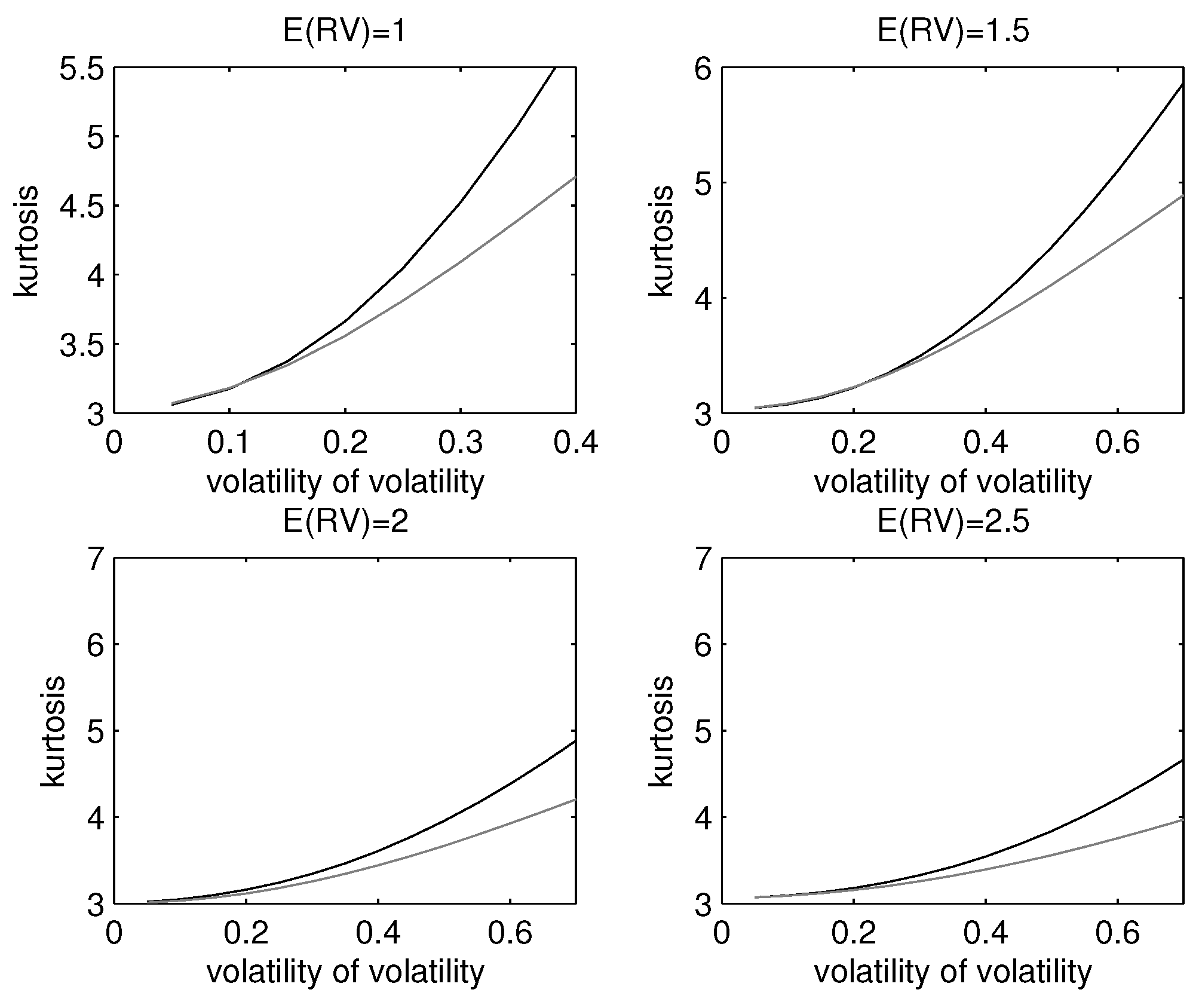
In Figure 1 and Figure 2, we illustrate the impact of volatility risk of the distribution of returns. For low values of the volatility of volatility (or more generally, for a low conditional coefficient of variation in volatility), the distribution of returns is still very close to the Gaussian case. This is consistent with the evidence that returns standardized by the realized volatility are nearly normally distributed: since the impact of the volatility of volatility is non-linear and grows slowly with the variable, the effect of errors in the underlying realized volatility estimator are not enough to generate excess kurtosis on the scaled returns. Figure 1 illustrates the consequences of the non-Gaussianity on the distribution of realized volatility shocks, where we assume a positively skewed and leptokurtic distribution with parameters calibrated with the S&P 500 data. The excess kurtosis on the volatility amplify the excess kurtosis on returns for a given volatility risk level.

Figure 1. The kurtosis of the simulated distribution under the assumption that shocks to realized volatilityhave the normal inverse Gaussian (NIG) (upper line) and normal distributions.

Figure 1. The kurtosis of the simulated distribution under the assumption that shocks to realized volatilityhave the normal inverse Gaussian (NIG) (upper line) and normal distributions.

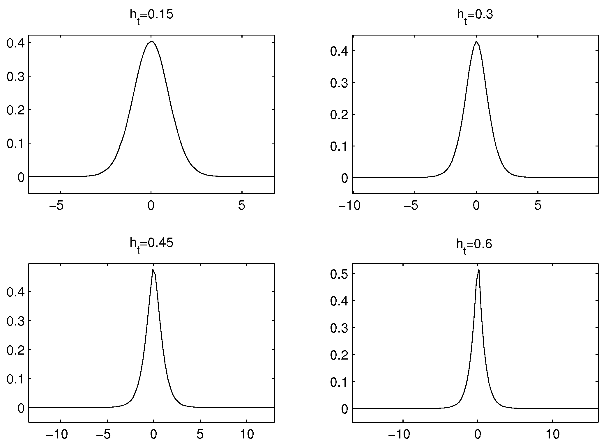
Figure 2. Densities for the simulated distributions (no volatility feedback).

Figure 2. Densities for the simulated distributions (no volatility feedback).

If the ${\epsilon }_t$ and ${\eta }_t$ are dependent, then trivially $E\left(r_t^3\right)=E\left({\sigma }^3\right)E\left({\epsilon }_t^3\right)=0$, so that in this type of model, the observed negative skewness on the ex ante distribution of returns must come from the negative dependence between ${\epsilon }_t$ and ${\eta }_t$. Writing the expression for the third moment,

$$E\left(r_t^3\right)=E(3{\psi }_t^2{h}_t{\eta }_t{\epsilon }_t^3+3{\psi }_t{h}_t^2{\eta }_t^2{\epsilon }_t^3+h_t^3{\eta }_t^3{\epsilon }_t^3)$$

(7)

which is not particularly illuminating, but highlights the fact that given the dependence structure between the two shocks, a higher volatility risk will also increase the conditional skewness in the returns.

Finally, if we choose to model the log of the realized variance ($log\left({\sigma }_t^2\right)={\psi }_t+h_t{\eta }_t$), we obtain:

$$E\left(r_t^2\right)=E\left({\sigma }_t^2\right)E\left({\epsilon }_t^2\right)=exp\left({\psi }_t\right)E(exp\left(h_t{\eta }_t\right))$$

(8)

$$\begin{array}{cc}\hfill \frac{E\left(r_t^4\right)}{E{\left(r_t^2\right)}^2}& =3\frac{E(exp2h_t{\eta }_t)}{{\left[E(exp{h}_t{\eta }_t)\right]}^2}\hfill \end{array}$$

(9)

In this case, both the conditional variance and the conditional kurtosis depend on the distribution of ${\eta }_t$. For example, if ${\eta }_t$ is assumed normal, the standard formula for the moment generating function of the normal distribution gives a conditional variance of $exp({\psi }_t+h_t^2/2)$ and a kurtosis $3exp\left(2h_t^2\right)$.

This analysis provides the ingredients for adequately modeling the empirically relevant ex ante distribution of returns in a stochastic volatility framework: the conditional mean of volatility, the volatility risk, the distribution of the shocks to volatility and the dependence structure between the shocks to returns and the shocks to volatility. The volatility risk parameter is an extremely important quantity in the model, as it is the main determinant of the excess kurtosis in the conditional distribution of returns and amplifies the negative conditional skewness in the returns. For risk management, option pricing and other applications where the full conditional distribution of returns is the object of interest, understanding and modeling this volatility risk is therefore fundamental.

The realized volatility literature so far has been mostly concerned with the conditional mean of volatility, and this is the gap the we intend to fill with the model of the next section. Our main argument is that the availability of realized volatility allows not only for significant advances in modeling the conditional volatility of returns, but also the higher moments of this distribution. The reason is straightforward: since realized volatility is an observable quantity, it is much easier to model and estimate the volatility of realized volatility than the tail heaviness parameter from return data in GARCH or stochastic volatility models. With realized volatility, we do not have to rely only on rare realizations in returns to identify the tails of the conditional return distribution. This becomes even more relevant in the presence of conditional heteroskedasticity in realized volatility, since identifying time-varying kurtosis in a GARCH setting is very hard [18,19].

An intuitive example further clarifies this point. Suppose we observe at a particular day a realized volatility of 10 and a return of zero. The return provides no information about the tails of the conditional return distribution for a GARCH or another latent variable model. However if we accept that returns given volatility are normally distributed and assume that return and volatility shocks are uncorrelated, then we have learned that on this particular day, the “ex post 1% value at risk” was $-2.326\times 10$, that is, an event comparable with the 19 October 1987, crash in the Dow Jones index could have happened at the tail, according to the model. Naturally, days of very high volatility are far more frequent than days of very high volatility and tail return shocks.

2.1. Volatility Risk: Empirical Regularities

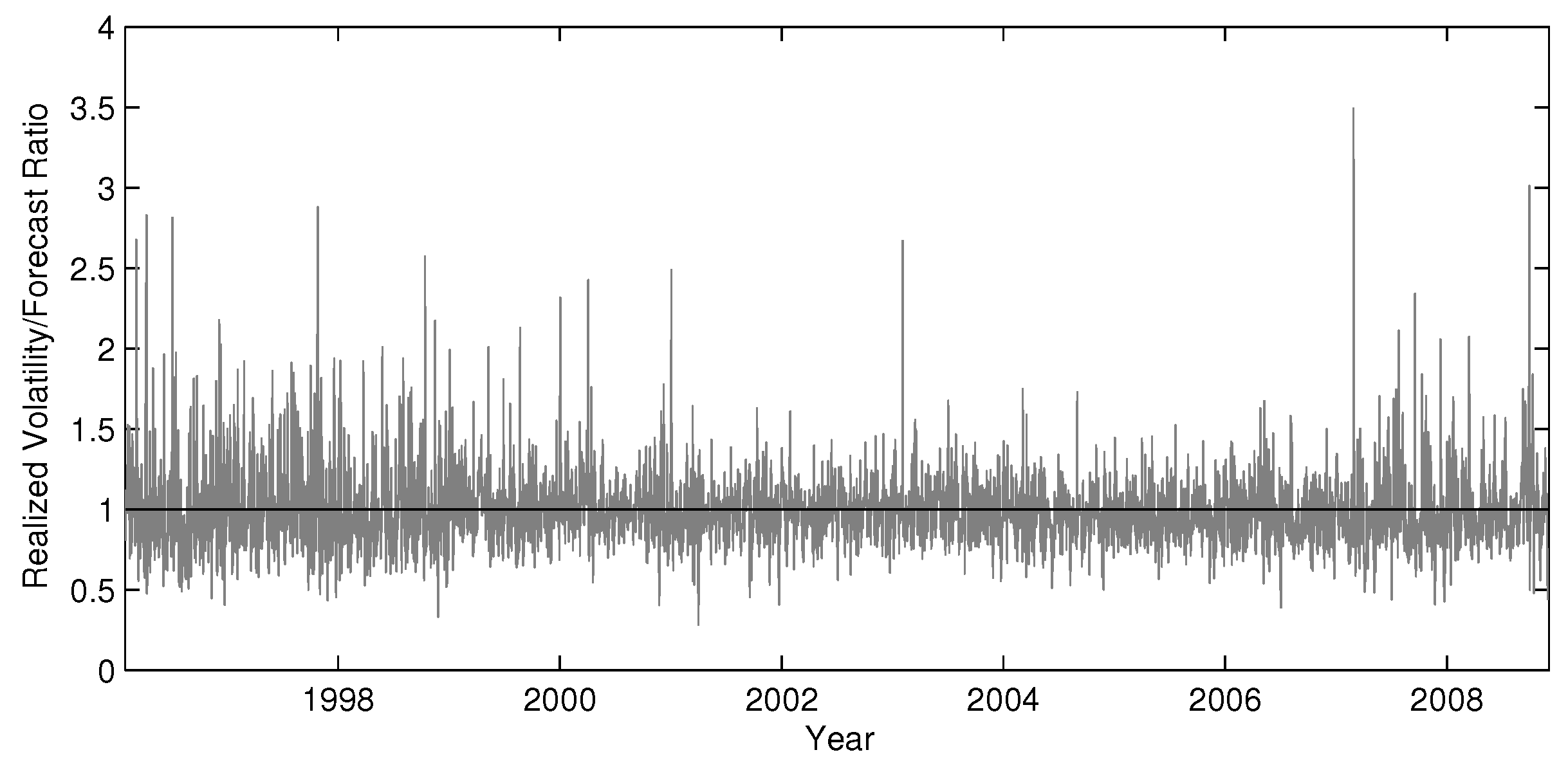
Volatility risk is a substantive issue empirically. This is illustrated more systematically by Table 1, which displays for a number of different series the sample statistics of the ratio between the in-sample realized volatility forecasts calculated from the best fitting model of the empirical study in Section 4 and the measured realized volatilities. The reader is referred to Section 4.1 for details on the data and realized volatility measurement. The ratio is extremely skewed to the right. For the S&P 500 index, at 10% of time, the actual volatility exceeds the forecast by approximately 30%, and at 1% of time, the actual volatility exceeded the prediction by 80%. In a setting with out-of-sample uncertainty, we can expect these values to be even higher. Figure 3 shows the high magnitude of the percentage forecasting errors in realized volatility for the S&P 500 index. Table 2 shows the descriptive statistics for the returns scaled by these volatility predictions. As our analysis suggested, Table 2 reveal a substantial degree of excess kurtosis for all series. For the indexes (but not the stocks), the distribution is pronouncedly negatively skewed, due to the volatility feedback effect.

Table 1. Descriptive statistics for $R{V}_t/{\widehat{RV}}_t$ ratios. WMT, Wal-Mart.

	Mean	SD	Skewness	Kurtosis	$Q_{0.75}$	$Q_{0.9}$	$Q_{0.95}$	$Q_{0.99}$
S&P 500	1.00	0.25	1.86	12.17	1.11	1.28	1.43	1.84
DJIA	1.01	0.30	1.94	15.52	1.15	1.35	1.53	1.95
FTSE	1.00	0.33	2.97	27.12	1.13	1.37	1.55	2.14
CAC	1.00	0.25	2.14	21.84	1.12	1.29	1.41	1.76
Nikkei	1.00	0.27	1.19	6.72	1.14	1.33	1.47	1.86
IBM	1.00	0.22	1.13	6.96	1.11	1.25	1.38	1.72
GE	1.00	0.20	0.85	5.30	1.11	1.25	1.37	1.63
WMT	1.00	0.24	1.25	7.82	1.12	1.29	1.41	1.74
AT&T	1.00	0.27	1.67	10.25	1.12	1.32	1.48	1.87

Table 1. Descriptive statistics for $R{V}_t/{\widehat{RV}}_t$ ratios. WMT, Wal-Mart.

	Mean	SD	Skewness	Kurtosis	$Q_{0.75}$	$Q_{0.9}$	$Q_{0.95}$	$Q_{0.99}$
S&P 500	1.00	0.25	1.86	12.17	1.11	1.28	1.43	1.84
DJIA	1.01	0.30	1.94	15.52	1.15	1.35	1.53	1.95
FTSE	1.00	0.33	2.97	27.12	1.13	1.37	1.55	2.14
CAC	1.00	0.25	2.14	21.84	1.12	1.29	1.41	1.76
Nikkei	1.00	0.27	1.19	6.72	1.14	1.33	1.47	1.86
IBM	1.00	0.22	1.13	6.96	1.11	1.25	1.38	1.72
GE	1.00	0.20	0.85	5.30	1.11	1.25	1.37	1.63
WMT	1.00	0.24	1.25	7.82	1.12	1.29	1.41	1.74
AT&T	1.00	0.27	1.67	10.25	1.12	1.32	1.48	1.87

Figure 3. In-sample percentage errors for the HAR (heterogeneous autoregressive) model with leverage effects.

Figure 3. In-sample percentage errors for the HAR (heterogeneous autoregressive) model with leverage effects.

Table 2. Descriptive statistics for returns standardized by in-sample realized volatility fitted  values.

	Mean	SD	Skewness	Kurtosis	$Q_{0.01}$
S&P 500	−0.019	1.061	−0.392	4.305	−2.780
DJIA	0.019	1.090	−0.340	3.944	−2.867
FTSE	−0.009	1.147	−0.177	3.694	−2.905
CAC	−0.011	1.053	−0.182	3.346	−2.654
Nikkei	−0.054	1.083	−0.152	3.715	−2.832
IBM	0.035	1.033	−0.076	4.505	−2.539
GE	−0.025	1.012	0.026	3.897	−2.479
WMT	−0.039	1.001	0.066	3.909	−2.432
AT&T	−0.037	1.028	0.024	4.397	−2.523

Table 2. Descriptive statistics for returns standardized by in-sample realized volatility fitted  values.

	Mean	SD	Skewness	Kurtosis	$Q_{0.01}$
S&P 500	−0.019	1.061	−0.392	4.305	−2.780
DJIA	0.019	1.090	−0.340	3.944	−2.867
FTSE	−0.009	1.147	−0.177	3.694	−2.905
CAC	−0.011	1.053	−0.182	3.346	−2.654
Nikkei	−0.054	1.083	−0.152	3.715	−2.832
IBM	0.035	1.033	−0.076	4.505	−2.539
GE	−0.025	1.012	0.026	3.897	−2.479
WMT	−0.039	1.001	0.066	3.909	−2.432
AT&T	−0.037	1.028	0.024	4.397	−2.523

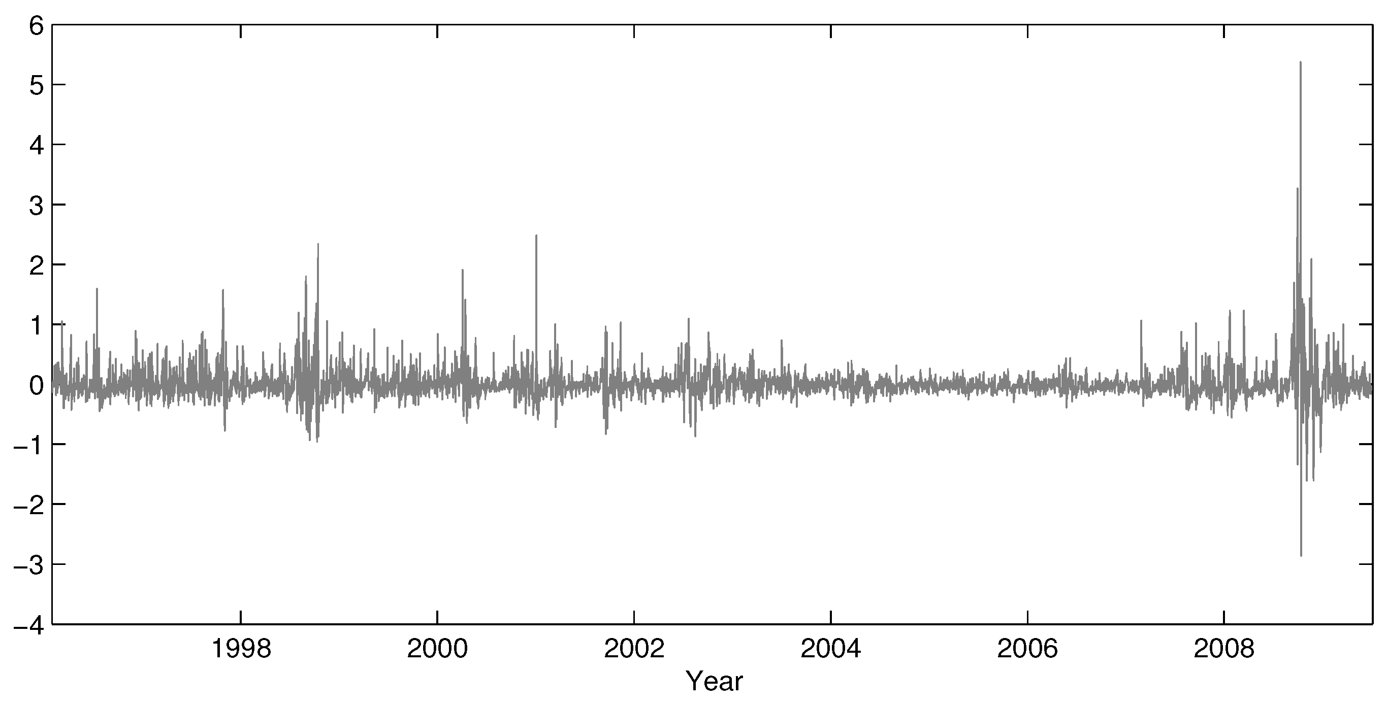
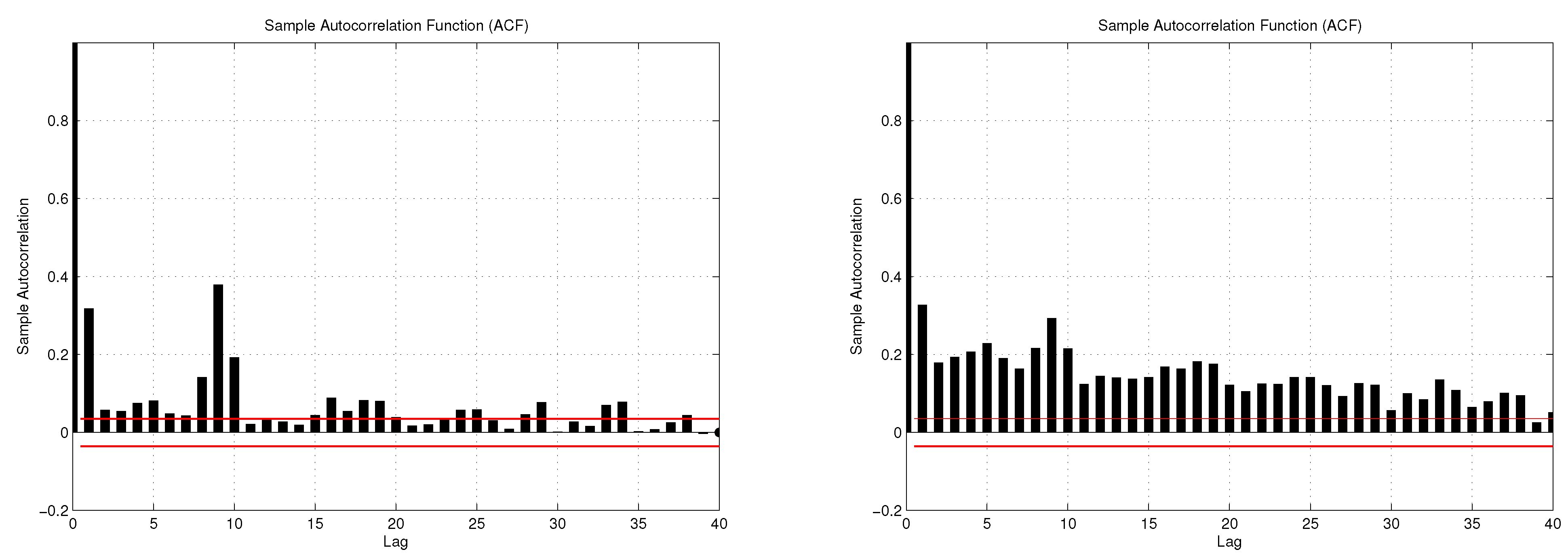
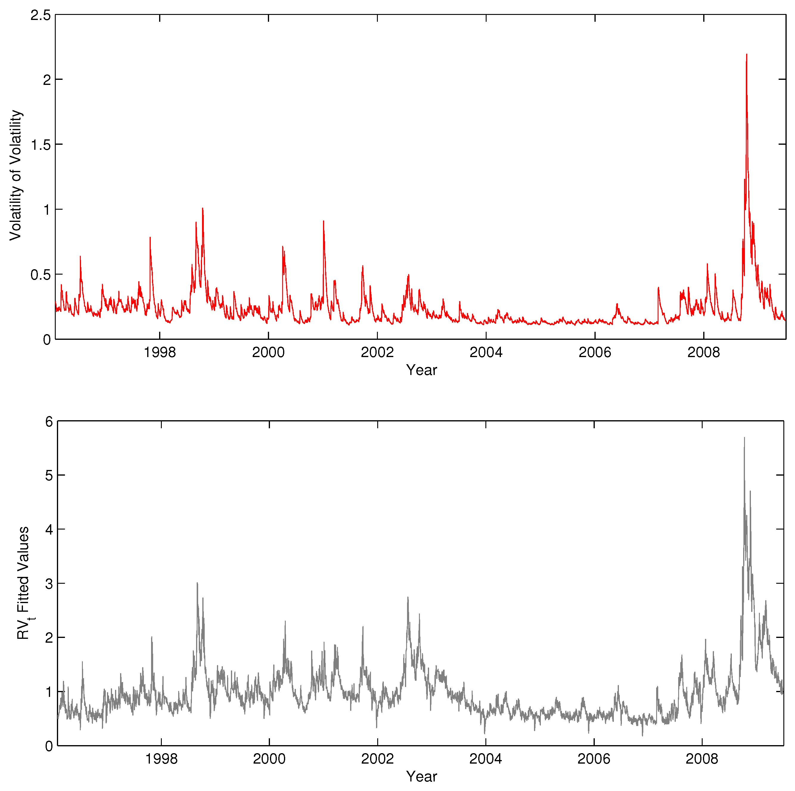
We now consider the time series properties of the volatility of realized volatility. Figure 4 shows the residuals of the HAR model for realized volatility considered in Corsi et al. [1]. Figure 5 displays the sample autocorrelations for the squared and absolute residuals. The figures provide unambiguous evidence for the presence of conditional heteroskedasticity in realized volatility, in line with Corsi et al. [1], Bollerslev et al. [4] and other previous studies. Figure 6 shows a pattern common to all our series: when we extend the model with a GARCH(1,1) specification for the residuals, as would be natural to account for this conditional heteroskedasticity in this case, there is always a strong relation between the estimated conditional volatility of realized volatility and the fitted values of the model. Thus, there seems to be a close positive association between volatility risk and the level of volatility. This is a new finding in the volatility literature, even though this relation has been explored many times before in the context options pricing (see, for example, [2,3]). This stylized fact motivates the new model presented in the next section.

Figure 4. Residuals series of the HAR model with leverage effects.

Figure 4. Residuals series of the HAR model with leverage effects.

Figure 5. Sample autocorrelations for the squared (left) and absolute (right) residuals of the HAR model with leverage effects.

Figure 5. Sample autocorrelations for the squared (left) and absolute (right) residuals of the HAR model with leverage effects.

Figure 6. GARCHstandard deviation series (top) and realized volatility fitted values (bottom) for the HAR model with leverage effects.

Figure 6. GARCHstandard deviation series (top) and realized volatility fitted values (bottom) for the HAR model with leverage effects.

3. The Dually Asymmetric Realized Volatility Model

The dually asymmetric realized volatility (DARV) model is a step in analyzing and incorporating the modeling qualities of a more realistic specification of the volatility risk within a standard realized volatility model. The dual asymmetry in the model comes from leverage effects (as seen in the last section) and the positive relation between the level of volatility and the degree of volatility risk. The fundamental issue that arises in specifying the model is how to specify the relation between the volatility level and risk.

We directly model the time series of realized volatility ($R{V}_t$), as we justify in Section 3.2. To be consistent with the notation of the last section, let the conditional variance of the residuals be denoted by $h_t^2$. In this paper, we choose the specification $h_t^2={\theta }_0+{\theta }_{1}V{L}_t^2$, where $V{L}_t$ (the volatility level) is the conditional mean of volatility ($E\left(R{V}_t\right|{\mathcal{F}}_{t-1})$, where ${\mathcal{F}}_{t-1}$ is the information set at end of the previous day). Another option would be to directly allow for the asymmetry of positive or negative shocks in volatility in a GARCH model, but we have found our simpler specification to perform better. A possibility for extending our specification would be to model the nonlinearities in the volatility level/risk relation, but more complicated specifications of this type are out of the scope of this paper.

The general specification of our model in autoregressive fractionally integrated and heterogeneous autoregressive versions are:

$$\begin{array}{cc}& \mathbf{DARV}\mathbf{-}\mathbf{FIModel}:\hfill \\ & r_t={\mu }_t+R{V}_t{\epsilon }_t,\hfill \\ & \varphi \left(L\right){(1-L)}^d(R{V}_t-{\psi }_t)={\lambda }_{1}I(r_{t-1}<0)r_{t-1}+{\lambda }_{2}I(r_{5,t-1}<0)r_{5,t-1}\hfill \\ & +{\lambda }_{3}I(r_{22,t-1}<0)r_{22,t-1}+h_t{\eta }_t\hfill \\ & h_t^2={\theta }_0+{\theta }_{1}V{L}_t^2\hfill \\ \\ & \mathbf{DARV}\mathbf{-}\mathbf{HAR}\mathbf{Model}:\hfill \\ & r_t={\mu }_t+R{V}_t{\epsilon }_t,\hfill \\ & R{V}_t={\varphi }_0+{\varphi }_{1}R{V}_{t-1}+{\varphi }_{2}R{V}_{5,t-1}+{\varphi }_{3}R{V}_{22,t-1}\hfill \\ & +{\lambda }_{1}I(r_{t-1}<0)r_{t-1}+{\lambda }_{2}I(r_{5,t-1}<0)r_{5,t-1}\hfill \\ & +{\lambda }_{3}I(r_{22,t-1}<0)r_{22,t-1}+h_t{\eta }_t\hfill \\ & h_t^2={\theta }_0+{\theta }_{1}V{L}_t^2\hfill \end{array}$$

(10)

where $r_t$ is the log return at day t, ${\mu }_t$ is the conditional mean for the returns, $R{V}_t$ is the realized volatility, ${\epsilon }_t$ is i.d.$N(0,1)$, ${\psi }_t$ shifts the unconditional mean of realized volatility, d denotes the fractional differencing parameter, $\Phi \left(L\right)$ is a polynomial with roots outside the unit circle, L the lag operator, I is the indicator function, $r_{j,t-1}$ is a notation for the cumulated returns ${\sum }_{i=t-j}^{t-1}{r}_{t-i}$, $R{V}_{j,t-1}={\sum }_{i=t-j}^{t-1}R{V}_{t-i}$, $h_t$ is the volatility of the realized volatility, ${\eta }_t$ is i.i.d. with $E\left({\eta }_t\right)=0$ and $E\left({\eta }_t^2\right)=1$, ${\epsilon }_t$ and ${\eta }_t$ are allowed to be dependent and $V{L}_t=E\left(R{V}_t\right|{\mathcal{F}}_{t-1})$.

3.1. Model Details

3.1.1. Long Memory Specification

Following the evidence of fractional integration in realized volatility, ARFIMA models are the standard in the literature. Fractionally integrated models have been estimated, for example, in Andersen et al. [6], Areal and Taylor [11], Beltratti and Morana [20], Deo et al. [21], Martens et al. [22], Thomakos and Wang [23], among others. Nevertheless, the estimation of ARFIMA models in this context has encountered a few shortcomings. Although $I\left(d\right)$ processes are a seemingly reasonable approximation for the data generating process of volatility series, there is no underlying theory to formally support this specification. Instead, the results of Diebold and Inoue [24] and Granger and Hyung [25] challenge fractional integration as the correct specification for realized volatility series by showing that long memory properties can be engendered by structural breaks or regime switching. ¹ Statistical tests for distinguishing between those alternatives, such as the one proposed Ohanissian et al. [30], have been hampered by low power. Finally, Granger and Ding [31] and Scharth and Medeiros [5] discuss how estimates of the fractional differencing parameter are subject to excessive variation over time.

Given the lack of stronger support for a strict interpretation of fractional integration evidence and the higher computational burden in estimating and forecasting this class of models, some researchers have chosen to apply simpler time series models, which are consistent with high persistence over the relevant horizons (like the HAR model of the last section), even though they do not rigorously exhibit long memory (hence, being labeled ‘quasi-long memory’ models). Since this debate bears little relevance for our analysis, we have chosen to present the dually asymmetric model in both a fractionally integrated version and a HAR version. After preliminary specification tests using the Schwarz criterion, we have selected an ARFIMA(1,d,0) model specification throughout this paper.

3.1.2. Extended Leverage Effects

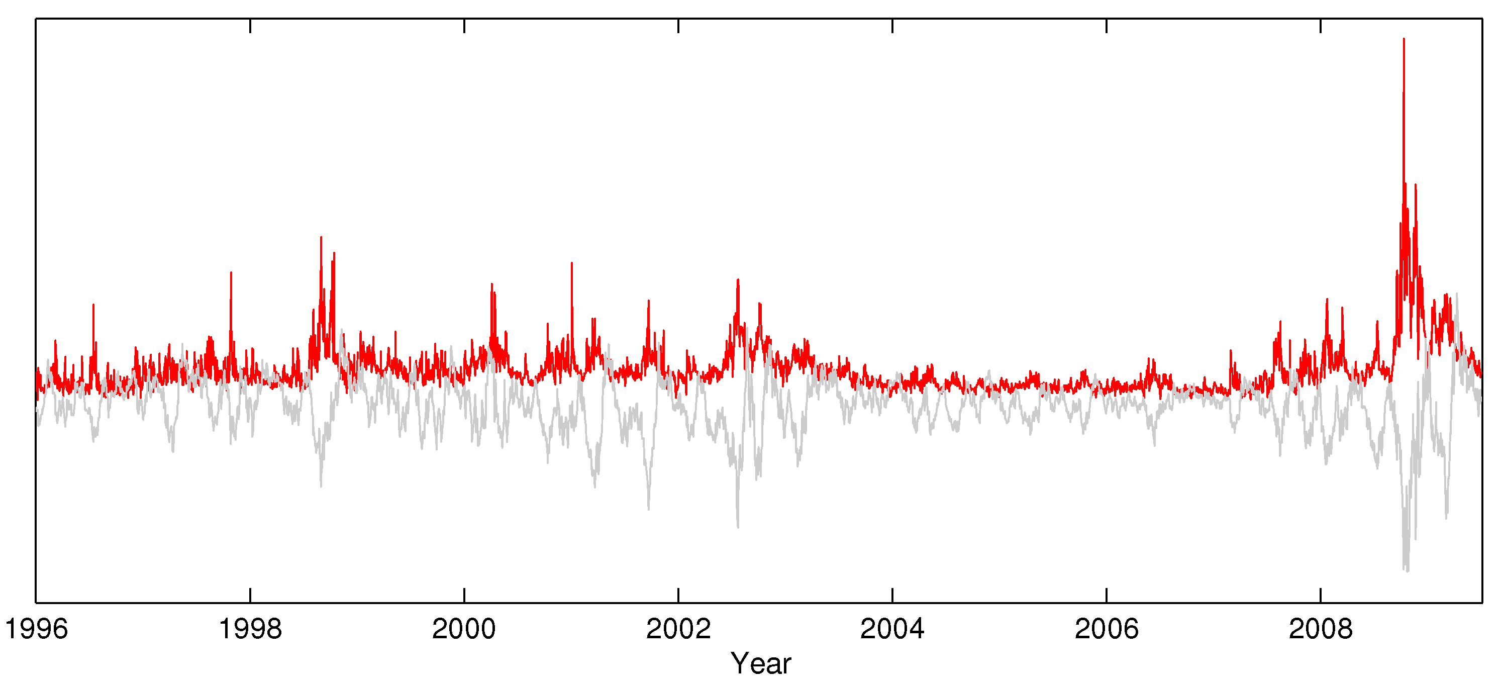
Bollerslev et al. [32] and Scharth and Medeiros [5] highlight the impact of leverage effects for the dynamics of realized volatility. The latter argues for the existence of regime switching behavior in volatility, with large falls (rises) in prices being associated with persistent regimes of high (low) variance in stock returns. The authors show that the incorporation of cumulated daily returns as a explanatory variable brings some modeling advantages by capturing this effect. While Scharth and Medeiros [5] consider multiple regimes in a nonlinear model, we focus on a simpler linear relationship to account for the large correlation between past cumulated returns and realized volatility. This extended leverage effect is shown in Figure 7, which plots the time series of S&P 500 realized volatility and monthly returns (re-scaled). The sample correlation between the two series is $-0.52$. It seems that virtually all episodes of (persistently) high volatility are associated with streams of negative returns; once the index price recovers, the realized volatility tends to quickly fall back to average levels.

Figure 7. Realized volatility (top) and monthly returns (bottom) for the S&P 500 index.

Figure 7. Realized volatility (top) and monthly returns (bottom) for the S&P 500 index.

3.1.3. The Distribution of the Volatility Disturbances

To account for the non-Gaussianity in the error terms, we follow Corsi et al. [1] and assume that the i.i.d. innovations ${\eta }_t$ follow the standardized normal inverse Gaussian (which we denote by $NI{G}^{*}$), which is flexible enough to allow for excessive kurtosis and skewness and reproduces a number of symmetric and asymmetric distributions. A more complex approach would rely on the generalized hyperbolic distribution, which encompasses the NIG distribution and requires the estimation of an extra parameter. On the other hand, typical distributions with support on the interval $(0,\infty )$, which would be a desirable feature for our case, were strongly rejected by preliminary diagnostic tests.

Finally, to model the asymmetry in the conditional return distribution, we let ${\eta }_t$ and ${\epsilon }_t$ be dependent and model this dependence via a bivariate Clayton copula. The copula approach is a straightforward way to account for non-linearities in this dependence relation and has the important advantage of not requiring the joint estimation of the return and volatility equations. Let $U=\Phi \left({\epsilon }_t\right)$ and $V=1-\mathsf{{\rm Y}}\left({\nu }_t\right)$, where $\Phi (.)$ and $\mathsf{{\rm Y}}(.)$ are the corresponding normal and $NI{G}^{*}$ cdfs for ${\epsilon }_t$ and ${\eta }_t$ respectively. The joint cdf or copula of U and V is given by:

$$\begin{array}{c}\hfill C_{\kappa }\equiv P(U\le u,V\le v)={\left(u^{-\kappa }+v^{-\kappa }-1\right)}^{-1/\kappa }\end{array}$$

(11)

In this simple copula specification, returns and volatility are negatively correlated and display lower tail dependence (days of very low returns and very high volatility are linked, where the strength of this association is given by the parameter κ).

3.1.4. Days-of-the-Week and Holiday Effects

To reduce bias on our estimators and avoid distortions of the error distribution, we control the mean of the dependent variable for day of the week and holiday effects using dummies. Martens et al. [11] and Scharth and Medeiros [5] show that volatility sometimes tend to be lower on Mondays and Fridays, while substantially less volatility is observed around certain holidays.

3.2. The Impact of Microstructure Noise and Other Issues

Our analysis ignores the presence of remaining measurement errors in volatility. Though standard in this literature, this may be an important omission, as it will lead us to overestimate the time series volatility of volatility. Additionally, the theory of realized volatility estimation indicates that the variance of the realized variance estimator is positively related to the integrated variance itself (see, for example, [33]). Regarding this problem, we offer the following remarks: (i) our use of the efficient realized kernel estimator of Barndorff-Nielsen et al. [34] in the next section minimizes the impact of microstructure noise for our results; (ii) the theory of Section 2 implies that the presence of large measurement noise should cause excess kurtosis in the returns scaled by realized volatility. To the extent that empirically these scaled returns are actually platykurtic (see Table 3), but returns standardized by realized volatility forecasts are highly leptokurtic (Table 2), we can be confident that our analysis is mostly capturing true volatility risk and not the estimator variance; (iii) as mentioned previously, the positive relation between the volatility level and volatility risk is confirmed by the options literature; and (iv) the variance of the realized volatility estimator is a source of modeling risk, with similar impacts for applications of realized volatility models.

Table 3. Descriptive statistics: S&P 500.

Statistic	$r_t$	${RV}_t$	$r_t/{RV}_t$	$\Delta {RV}_t$
Mean	0.012	0.984	0.042	0.000
SD	1.343	0.605	1.013	0.359
Skewness	−0.186	3.417	0.040	−0.913
Kurtosis	10.570	26.342	2.743	65.184
Min	−9.470	0.212	−3.296	−6.840
$Q_{0.1}$	−1.443	0.478	−1.282	−0.308
$Q_{0.25}$	−0.610	0.606	−0.658	−0.135
$Q_{0.75}$	0.654	1.153	0.711	0.127
$Q_{0.9}$	1.368	1.584	1.382	0.301
Max	10.957	9.673	3.230	5.280

Table 3. Descriptive statistics: S&P 500.

Statistic	$r_t$	${RV}_t$	$r_t/{RV}_t$	$\Delta {RV}_t$
Mean	0.012	0.984	0.042	0.000
SD	1.343	0.605	1.013	0.359
Skewness	−0.186	3.417	0.040	−0.913
Kurtosis	10.570	26.342	2.743	65.184
Min	−9.470	0.212	−3.296	−6.840
$Q_{0.1}$	−1.443	0.478	−1.282	−0.308
$Q_{0.25}$	−0.610	0.606	−0.658	−0.135
$Q_{0.75}$	0.654	1.153	0.711	0.127
$Q_{0.9}$	1.368	1.584	1.382	0.301
Max	10.957	9.673	3.230	5.280

We have chosen to specify a linear model for the realized volatility, even though a log specification is more common in the realized volatility literature. Corsi et al. [35] and Bollerslev et al. [4] show that the log transformation is not enough to fully account for the heteroskedasticity in volatility. The reason we work with the level is that the log transformation by construction obscures the volatility level/risk association, which we consider to be an important relationship to be modeled. The empirical results of Section support this view. We have the following additional comments: (i) in contrast with most previous studies our interest lies in the distribution of the $R{V}_t$ itself, which we therefore model directly; (ii) there is virtually no loss forecasting of performance on modeling the level (see, for example, [1]); and (iii) the fact that the estimated error distribution is very right skewed and the conditional variance of $RV$ shrinks with the level of the variable eliminates the possibility of negative volatility in the model for all practical purposes in our data.

In contrast with Bollerslev et al. [4], which also considers a full system for returns, realized volatility and the volatility of volatility, our model does not consider jump components in the realized volatility. ² The use of jumps does not seem to bring important forecasting advantages in our framework. On the other hand, the inclusion of a jump equation would substantially increase the complexity of the model, requiring us to model and estimate the joint distribution of return, volatility and jump shocks. For predicting and simulating the model multiple periods ahead, this is a substantial burden. Since the ultimate interest lies in the conditional distribution of returns, a parsimonious alternative is to ignore the distinction between continuous and jump components in realized volatility and to carefully model the distribution of returns given realized volatility (considering the possible impact of jumps on it). Corsi and Reno (2012) provides some evidence that the impact of jumps on volatility is quite transitory.

3.3. Estimation and Density Forecasting

We estimate the two versions of the dually asymmetric realized volatility model by maximum likelihood. The fact that the conditional volatility of volatility $h_t$ depends on the conditional mean of the realized volatility brings no issues for the estimation. However, a full maximum likelihood procedure for the ARFIMA model (e.g., Sowell [37]) is unavailable under the assumptions of conditional heteroskedasticity and the NIG distribution for the errors ${\eta }_t$. We then follow the standard approach in the literature and turn to a consistent approximate maximum likelihood procedure where the fractional differencing operator ${(1-L)}^d$ is replaced by a truncation of its corresponding binomial expansion.³ The use of this approximate estimator does not impact, in any away, the main arguments of this paper. For reference, the log-likelihood function is given by:

$$\begin{array}{c}\hfill \ell (\widehat{d},\widehat{\varphi },\widehat{\psi },\widehat{\lambda },\widehat{\theta },\widehat{\alpha },\widehat{\beta };R{V}_{1...T},X_{1...T})=Tlog\left(\widehat{\alpha }\right)-Tlog\left(\pi \right)+\sum _{t=1}^{T}log\left[K_1\left(\widehat{\alpha }\widehat{\delta }{(1+{\widehat{y}}_t^2)}^{1/2}\right)\right]\\ \hfill -0.5\sum _{t=1}^{T}log(1+{\widehat{y}}_t^2)+T\widehat{\delta }{({\widehat{\alpha }}^2-{\widehat{\beta }}^2)}^{1/2}+\widehat{\delta }\widehat{\beta }\sum _{t=1}^T{\widehat{y}}_t-0.5\sum _{t=1}^{T}log\left({\widehat{h}}_t\right)\end{array}$$

(12)

where X collects the additional explanatory variables, α and β are the tail heaviness and asymmetry parameters of the standardized NIG distribution. $\gamma ={({\widehat{\alpha }}^2-{\widehat{\beta }}^2)}^{1/2}$ and ${\widehat{y}}_t=\frac{{\widehat{\eta }}_t/{\widehat{h}}_t-\widehat{\omega }}{\widehat{\delta }}$, where ω and δ are the location and scale parameters associated with the standardized NIG distributed with parameters α and β.

The copula specification for the joint distribution of return and volatility innovations allows us to estimate the copula by maximum likelihood in a separate stage once we have obtained estimates for ${\eta }_t$ and ${\epsilon }_t$ from the marginal models. For simplicity, we estimate the mean of returns ${\mu }_t$ by the sample mean (since the daily expected return is very small, ${\mu }_t$ is immaterial for our analysis), so that $\widehat{{\epsilon }_t}=(r_t-\widehat{\mu })/R{V}_t$.

An analytical solution for the return density implied by our flexible normal variance-mean mixture hypothesis (realized volatility is distributed normal inverse Gaussian, and returns given volatility are normally distributed) is not available. Except for a few cases, such as one day ahead point forecasts for realized volatility, many quantities of interest based on our model have to be obtained by simulation. We consider the following Monte Carlo method, which can be easily implemented and made accurate with realistic computational power. Conditional on information up to day t, we implement the following general procedure for simulating joint paths for returns and volatility (where ∼ is used to denote a simulated quantity):

• In the first step, the functional form of the model is used for the evaluation of forecasts ${\widehat{RV}}_{t+1}$ and ${\widehat{h}}_{t+1}$ conditional on past realized volatility observations, returns and other variables.
• Using the estimated copula, we randomly generate S pairs of return (${\tilde{\epsilon }}_{t+1,j}$, $j=1,..,S$) and volatility (${\tilde{\eta }}_{t+1,j}$, $j=1,..,S$) shocks with the according marginal distributions. Antithetic variables are used to balance the return innovations for location and scale.
• We obtain S simulated volatilities through ${\widetilde{RV}}_{t+1,j}={\widehat{RV}}_{t+1}+h_t{\tilde{\eta }}_{t+1,j}$, $j=1,...,S$. Each of these volatilities generate a returns ${\tilde{r}}_{t+1,j}={\widehat{\mu }}_t+{\widetilde{RV}}_{t+1,j}{\tilde{\epsilon }}_{t+1,j}$.
• This procedure can be iterated in the natural way to generate multiple paths for returns and realized volatility.

4. Empirical Analysis

4.1. Realized Volatility Measurement and Data

Suppose that at day t, the logarithmic prices of a given asset follow a continuous time diffusion:

$$dp(t+\tau )=\mu (t+\tau )+\sigma (t+\tau )dW(t+\tau ),0\le \tau \le 1,t=1,2,3...$$

where $p(t+\tau )$ is the logarithmic price at time $t+\tau$, is the drift component, $\sigma (t+\tau )$ is the instantaneous volatility (or standard deviation) and $dW(t+\tau )$ is a standard Brownian motion. Andersen et al. [6] and Barndorff-Nielsen and Shephard [33] showed that the daily compound returns, defined as $r_t=p\left(t\right)-p(t+1)$, are Gaussian conditionally on ${\mathcal{F}}_t=\sigma (p\left(s\right),s\le t)$, the σ-algebra (information set) generated by the sample paths of p, such that:

$$r_t|{\mathcal{F}}_t\sim N\left({\int }_0^1\mu (t-1+\tau )d\tau ,{\int }_0^1{\sigma }^2(t-1+\tau )d\tau \right)$$

The term $I{V}_t={\int }_0^1{\sigma }^2(t-1+\tau )d\tau$ is known as the integrated variance, which is a measure of the day t ex post volatility. In this sense, the integrated variance is the object of interest. In practical applications, prices are observed at discrete and irregularly-spaced intervals, and the most widely used sampling scheme is calendar time sampling (CTS), where the intervals are equidistant in calendar time. If we set $p_{i,t},i=1,..,n$ to be the i-th price observation during day t, realized variance is defined as ${\sum }_{i=1}^n{r}_{i,t}^2$. The realized volatility is the square-root of the realized variance, and we shall denote it by $R{V}_t$. Ignoring the remaining measurement error, this ex post volatility measure can be modeled as an “observable” variable, in contrast to latent variable models.

In real data, high frequency measures are contaminated by microstructure noise. The search for unbiased, consistent and efficient methods for measuring realized volatility has been one of the most active research topics in financial econometrics over the last few years. While early references, such as Andersen et al. [16], suggest the simple selection of an arbitrary frequency to balance accuracy and the dissipation of microstructure bias, a procedure known as sparse sampling, a number of recent articles developed estimators that dominate this procedure. In this paper, we turn to the theory developed by Barndorff-Nielsen et al. [34] and implement the consistent realized kernel estimator based on the modified Tukey–Hanning kernel. Some alternatives are the two time scale estimator of [38,39], the multiscale estimator of Zhang [40] and the pre-averaging estimator of Jacod et al. [41]. See McAleer and Medeiros [42] and Gatheral and Oomen [43] for a review and comparison of methods.

Our empirical analysis will focus on the realized volatility of the S&P 500 (SPX), Dow Jones (DJIA), FTSE100, CAC40 and Nikkei 225 indexes and the IBM, GE, Wal-Mart (WMT) and AT&T stocks. For conciseness, the S&P 500 index will be at the center of our analysis, with the other series being used when appropriate to show that our results hold more generally. The raw intraday data was obtained from the Reuters Datascope Tick History database and consists of tick by tick open to close quotes filtered for possible errors. For the S&P 500 index, we use the information originated in the E-Mini S&P500 futures market of the Chicago Mercantile Exchange, while for the remaining indexes, we use the actual index price series from different sources. ⁴ Following the results of Hansen and Lunde [44], we adopt the previous tick method for determining prices at time marks where a quote is missing.

The period of analysis starts on January 2, 1996, and ends on June 30, 2009, providing a total of 3,343 trading days in the United States. We clarify that our in-sample period used for revising the stylized facts, presenting the volatility risk findings and discussing the estimation diagnostics covers the whole sample, while the out-of-sample period used in Section 4 runs from 2001 to the end of the sample. We need our out-of-sample period to be unusually long, since the behavior of realized volatility markedly favors different kinds of models in particular years (for example, crisis periods strongly favor models with leverage effects), and a reasonable number of tail realizations are necessary to compare different alternatives for modeling volatility risk.

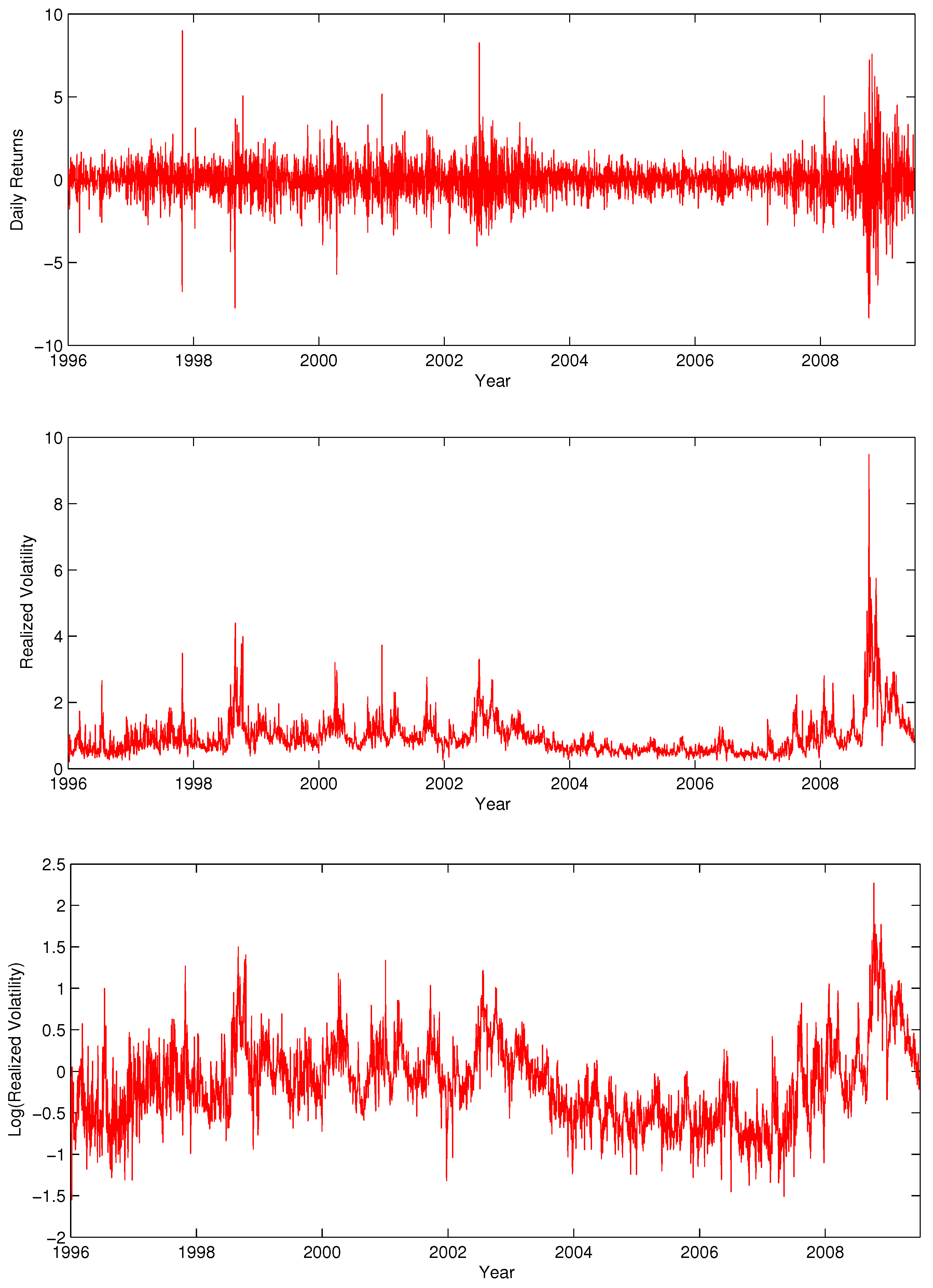
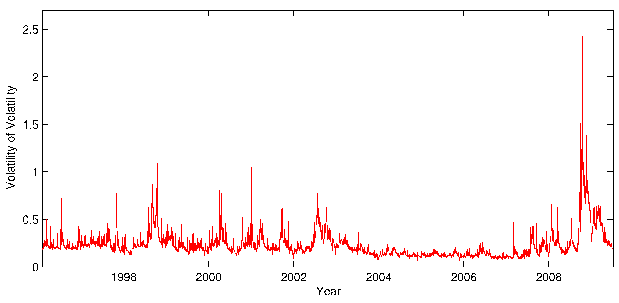
Figure 8 and Figure 9 display the time series of returns, realized volatility and log realized volatility, and the estimated volatility of realized volatility, respectively. Table 3 presents descriptive statistics for returns, standardized returns, realized volatility and changes in realized volatility. In light of our previous discussion, one striking feature of Table 3 is the extreme leptokurtosis in the realized volatility changes ($\Delta R{V}_t$). In fact, only 10% of observations account for close to 80% of the variation in realized volatility across the sample.

Figure 8. Time Series of returns (top), realized volatility (middle) and log realized volatility (bottom) for the S&P 500 index.

Figure 8. Time Series of returns (top), realized volatility (middle) and log realized volatility (bottom) for the S&P 500 index.

Figure 9. S&P500 estimated volatility of realized volatility.

Figure 9. S&P500 estimated volatility of realized volatility.

4.2. Full Sample Parameter Estimates and Diagnostics

We consider five alternative specifications chosen to illuminate the improvements introduced by different elements of the model: the homoskedastic ARFIMA(1,d,0) model with and without (extended) leverage effects, the ARFIMA-GARCH model with and without leverage effects and the HAR-GARCH model with leverage effects. We leave the simpler HAR specifications out of the analysis, as they are essentially redundant to the fractionally integrated counterparts. We consider the dependence between the return and volatility innovations on all specifications.

Table 4 and Table 5 show the parameter estimates for all of our specifications for the S&P 500 series. While most of the estimates are unexceptional and in line with the previous literature, we draw attention to two noteworthy results. First, in the ARFIMA setting, considering either conditional heteroskedasticity or extended leverage effects substantially changes our estimates for the fractional differencing parameter and the unconditional mean of realized volatility. Second, the leverage effect coefficients are significantly larger in the dually asymmetric estimations in comparison to other models. This interaction is likely to be consequential for our forecasting results.

Table 6 displays a variety of estimation diagnostics. Not surprisingly, the inclusion of leverage effects and time varying volatility risk considerably improve the fit of the specifications according to the Schwarz criterion and other standard statistics. The first piece of evidence in favor of the DARV model also comes from this analysis: our specification for the volatility risk unambiguously improving the fit of the model compared to the specifications with GARCH effects, though both alternatives seem to appropriately account for the autocorrelation in the squared residuals. On the other hand, an adverse result affecting all specifications comes from the (small) sample autocorrelation in the residuals. Reversing this result would require ad hoc modifications in our setting, leaving some role for more complex models or structural breaks to capture these dynamics.

Table 4. Estimated parameters (S&P 500): ARFIMAmodels. DARV, dually asymmetric realized volatility; AE, asymmetric effects.

Parameter	ARFIMA			ARFIMA + AE			ARFIMA-GARCH			ARFIMA + AE-GARCH			DARV-FI
ψ	0.989	(0.029)		0.653	(0.028)		0.970	(0.053)		0.546	(0.028)		0.400	(0.025)
d	0.340	(0.011)		0.261	(0.008)		0.464	(0.012)		0.352	(0.013)		0.367	(0.015)
${\varphi }_1$	0.064	(0.017)		0.033	(0.019)		−0.075	(0.017)		−0.047	(0.020)		−0.074	(0.019)
${\lambda }_1$	−	−		−0.055	(0.006)		−	−		−0.049	(0.005)		−0.072	(0.006)
${\lambda }_2$	−	−		−0.018	(0.003)		−	−		−0.012	(0.003)		−0.023	(0.004)
${\lambda }_3$	−	−		−0.014	(0.002)		−	−		−0.011	(0.002)		−0.013	(0.002)
${\theta }_0$	0.105	(0.005)		0.089	(0.006)		0.002	(0.000)		0.001	(0.000)		0.013	(0.001)
${\theta }_1$	−	−		−	−		−	−		−	−		0.101	(0.007)
${\theta }_2$	−	−		−	−		0.845	(0.018)		0.852	(0.015)		−	−
${\theta }_3$	−	−		−	−		0.127	(0.017)		0.121	(0.015)		−	−
α	0.906	(0.046)		0.855	(0.052)		1.841	(0.125)		1.663	(0.117)		1.800	(0.168)
β	0.548	(0.046)		0.479	(0.049)		1.075	(0.106)		0.910	(0.095)		1.037	(0.140)
κ	0.169	(0.024)		0.157	(0.023)		0.207	(0.024)		0.228	(0.024)		0.254	(0.025)

The table shows parameter estimates for different restrictions of the model: $(1-{\varphi }_{1}L){(1-L)}^d(R{V}_t-{\psi }_t)={\lambda }_{1}I(r_{t-1}<0)r_{t-1}+{\lambda }_{2}I(r_{5,t-1}<0)r_{5,t-1}+{\lambda }_{3}I(r_{22,t-1}<0)r_{22,t-1}+h_t{\eta }_t$, $h_t^2={\theta }_0+{\theta }_{1}V{L}_t^2+{\theta }_2{h}_{t-1}^2+{\theta }_3{\nu }_{t-1}^2$,${\eta }_t\sim NI{G}^{*}(\alpha ,\beta ),(\Phi \left({\epsilon }_t\right),1-\mathsf{{\rm Y}}\left({\eta }_t\right))\sim C_{clayton}^{\kappa }$.

Table 4. Estimated parameters (S&P 500): ARFIMAmodels. DARV, dually asymmetric realized volatility; AE, asymmetric effects.

Parameter	ARFIMA			ARFIMA + AE			ARFIMA-GARCH			ARFIMA + AE-GARCH			DARV-FI
ψ	0.989	(0.029)		0.653	(0.028)		0.970	(0.053)		0.546	(0.028)		0.400	(0.025)
d	0.340	(0.011)		0.261	(0.008)		0.464	(0.012)		0.352	(0.013)		0.367	(0.015)
${\varphi }_1$	0.064	(0.017)		0.033	(0.019)		−0.075	(0.017)		−0.047	(0.020)		−0.074	(0.019)
${\lambda }_1$	−	−		−0.055	(0.006)		−	−		−0.049	(0.005)		−0.072	(0.006)
${\lambda }_2$	−	−		−0.018	(0.003)		−	−		−0.012	(0.003)		−0.023	(0.004)
${\lambda }_3$	−	−		−0.014	(0.002)		−	−		−0.011	(0.002)		−0.013	(0.002)
${\theta }_0$	0.105	(0.005)		0.089	(0.006)		0.002	(0.000)		0.001	(0.000)		0.013	(0.001)
${\theta }_1$	−	−		−	−		−	−		−	−		0.101	(0.007)
${\theta }_2$	−	−		−	−		0.845	(0.018)		0.852	(0.015)		−	−
${\theta }_3$	−	−		−	−		0.127	(0.017)		0.121	(0.015)		−	−
α	0.906	(0.046)		0.855	(0.052)		1.841	(0.125)		1.663	(0.117)		1.800	(0.168)
β	0.548	(0.046)		0.479	(0.049)		1.075	(0.106)		0.910	(0.095)		1.037	(0.140)
κ	0.169	(0.024)		0.157	(0.023)		0.207	(0.024)		0.228	(0.024)		0.254	(0.025)

The table shows parameter estimates for different restrictions of the model: $(1-{\varphi }_{1}L){(1-L)}^d(R{V}_t-{\psi }_t)={\lambda }_{1}I(r_{t-1}<0)r_{t-1}+{\lambda }_{2}I(r_{5,t-1}<0)r_{5,t-1}+{\lambda }_{3}I(r_{22,t-1}<0)r_{22,t-1}+h_t{\eta }_t$, $h_t^2={\theta }_0+{\theta }_{1}V{L}_t^2+{\theta }_2{h}_{t-1}^2+{\theta }_3{\nu }_{t-1}^2$,${\eta }_t\sim NI{G}^{*}(\alpha ,\beta ),(\Phi \left({\epsilon }_t\right),1-\mathsf{{\rm Y}}\left({\eta }_t\right))\sim C_{clayton}^{\kappa }$.

Table 5. Estimated parameters (S&P 500): HAR models.

Parameter	HAR/AE-GARCH			DARV (HAR)
${\varphi }_0$	0.090	(0.008)		0.087	(0.009)
${\varphi }_1$	0.231	(0.016)		0.250	(0.016)
${\varphi }_2$	0.357	(0.017)		0.362	(0.022)
${\varphi }_3$	0.273	(0.016)		0.244	(0.018)
${\lambda }_1$	−0.052	(0.005)		−0.072	(0.006)
${\lambda }_2$	−0.016	(0.003)		−0.024	(0.004)
${\lambda }_3$	−0.007	(0.002)		−0.009	(0.002)
${\theta }_0$	0.001	(0.000)		0.001	(0.001)
${\theta }_1$	−	−		0.054	(0.003)
${\theta }_2$	0.853	(0.014)		−	−
${\theta }_3$	0.122	(0.014)		−	−
α	1.752	(0.136)		1.669	(0.149)
β	1.014	(0.116)		0.931	(0.121)
κ	0.242	(0.024)		0.272	(0.025)

The table shows parameter estimates for different restrictions of the model: $R{V}_t={\varphi }_0+{\varphi }_{1}R{V}_{t-1}+{\varphi }_{2}R{V}_{5,t-1}+{\varphi }_{3}R{V}_{22,t-1}$$+{\lambda }_{1}I(r_{t-1}<0)r_{t-1}+{\lambda }_{2}I(r_{5,t-1}<0)r_{5,t-1}+{\lambda }_{3}I(r_{22,t-1}<0)r_{22,t-1}+h_t{\eta }_t$, $h_t^2={\theta }_0+{\theta }_{1}V{L}_t^2+{\theta }_2{h}_{t-1}^2+{\theta }_3{\nu }_{t-1}^2$, ${\eta }_t\sim NI{G}^{*}(\alpha ,\beta ),(\Phi \left({\epsilon }_t\right),1-\mathsf{{\rm Y}}\left({\eta }_t\right))\sim C_{clayton}^{\kappa }$.

Table 5. Estimated parameters (S&P 500): HAR models.

Parameter	HAR/AE-GARCH			DARV (HAR)
${\varphi }_0$	0.090	(0.008)		0.087	(0.009)
${\varphi }_1$	0.231	(0.016)		0.250	(0.016)
${\varphi }_2$	0.357	(0.017)		0.362	(0.022)
${\varphi }_3$	0.273	(0.016)		0.244	(0.018)
${\lambda }_1$	−0.052	(0.005)		−0.072	(0.006)
${\lambda }_2$	−0.016	(0.003)		−0.024	(0.004)
${\lambda }_3$	−0.007	(0.002)		−0.009	(0.002)
${\theta }_0$	0.001	(0.000)		0.001	(0.001)
${\theta }_1$	−	−		0.054	(0.003)
${\theta }_2$	0.853	(0.014)		−	−
${\theta }_3$	0.122	(0.014)		−	−
α	1.752	(0.136)		1.669	(0.149)
β	1.014	(0.116)		0.931	(0.121)
κ	0.242	(0.024)		0.272	(0.025)

The table shows parameter estimates for different restrictions of the model: $R{V}_t={\varphi }_0+{\varphi }_{1}R{V}_{t-1}+{\varphi }_{2}R{V}_{5,t-1}+{\varphi }_{3}R{V}_{22,t-1}$$+{\lambda }_{1}I(r_{t-1}<0)r_{t-1}+{\lambda }_{2}I(r_{5,t-1}<0)r_{5,t-1}+{\lambda }_{3}I(r_{22,t-1}<0)r_{22,t-1}+h_t{\eta }_t$, $h_t^2={\theta }_0+{\theta }_{1}V{L}_t^2+{\theta }_2{h}_{t-1}^2+{\theta }_3{\nu }_{t-1}^2$, ${\eta }_t\sim NI{G}^{*}(\alpha ,\beta ),(\Phi \left({\epsilon }_t\right),1-\mathsf{{\rm Y}}\left({\eta }_t\right))\sim C_{clayton}^{\kappa }$.

Table 6. Estimation diagnostics (S&P 500).

	ARFIMA	ARFIMA + AE	ARFIMA GARCH	ARFIMA + AE GARCH	DARV (FI)	HAR + AE GARCH	DARV (HAR)
Log-Likelihood	292.34	455.29	757.00	882.31	955.65	870.12	915.38
$R^2$	0.688	0.723	0.739	0.778	0.789	0.778	0.787
BIC	−455.59	−749.20	−1,360.69	−1,579.05	−1,717.64	−1546.58	−1629.04
SD (${\widehat{\nu }}_t$)	0.323	0.295	0.312	0.288	0.281	0.288	0.283
Ljung–Box (1) (${\widehat{\nu }}_t$)	0.000	0.000	0.000	0.021	0.009	0.325	0.000
Ljung–Box (5) (${\widehat{\nu }}_t$)	0.000	0.000	0.000	0.000	0.000	0.000	0.000
Ljung–Box (10) (${\widehat{\nu }}_t$)	0.000	0.000	0.000	0.000	0.000	0.000	0.000
Skewness (${\widehat{\eta }}_t$)	4.58	3.86	1.63	1.68	2.02	1.64	1.95
Kurtosis (${\widehat{\eta }}_t$)	65.02	52.03	9.82	10.47	14.24	9.88	13.74
ARCH(1) (${\widehat{\eta }}_t$)	0.000	0.000	0.306	0.397	0.693	0.422	0.692
ARCH (5) (${\widehat{\eta }}_t$)	0.000	0.000	0.910	0.876	0.315	0.843	0.340
ARCH (10) (${\widehat{\eta }}_t$)	0.000	0.000	0.293	0.510	0.158	0.636	0.194
K-S Test (${\widehat{\eta }}_t$)	0.000	0.000	0.051	0.076	0.716	0.015	0.913
Ljung–Box (1) $(z-\overline{z})$	0.073	0.362	0.000	0.039	0.927	0.251	0.181
Ljung–Box (1) ${(z-\overline{z})}^2$	0.000	0.000	0.199	0.250	0.994	0.283	0.716
Ljung–Box (1) ${(z-\overline{z})}^3$	0.003	0.011	0.002	0.115	0.998	0.619	0.357
Ljung–Box (1) ${(z-\overline{z})}^4$	0.000	0.000	0.274	0.208	0.965	0.479	0.857

The table shows a variety of diagnostics for the estimations presented in Table 4 and Table 5. In the table, ${\widehat{\nu }}_t$ denote the estimated residuals and $\widehat{\eta }={\widehat{\nu }}_t/{\widehat{h}}_t=$ the standardized residuals. For the statistical tests in the table, the p-values are reported. K-S denotes the Kolmogorov–Smirnov Test. z is the probability integral transform of the standardized residuals using the estimated NIG distribution.

Table 6. Estimation diagnostics (S&P 500).

	ARFIMA	ARFIMA + AE	ARFIMA GARCH	ARFIMA + AE GARCH	DARV (FI)	HAR + AE GARCH	DARV (HAR)
Log-Likelihood	292.34	455.29	757.00	882.31	955.65	870.12	915.38
$R^2$	0.688	0.723	0.739	0.778	0.789	0.778	0.787
BIC	−455.59	−749.20	−1,360.69	−1,579.05	−1,717.64	−1546.58	−1629.04
SD (${\widehat{\nu }}_t$)	0.323	0.295	0.312	0.288	0.281	0.288	0.283
Ljung–Box (1) (${\widehat{\nu }}_t$)	0.000	0.000	0.000	0.021	0.009	0.325	0.000
Ljung–Box (5) (${\widehat{\nu }}_t$)	0.000	0.000	0.000	0.000	0.000	0.000	0.000
Ljung–Box (10) (${\widehat{\nu }}_t$)	0.000	0.000	0.000	0.000	0.000	0.000	0.000
Skewness (${\widehat{\eta }}_t$)	4.58	3.86	1.63	1.68	2.02	1.64	1.95
Kurtosis (${\widehat{\eta }}_t$)	65.02	52.03	9.82	10.47	14.24	9.88	13.74
ARCH(1) (${\widehat{\eta }}_t$)	0.000	0.000	0.306	0.397	0.693	0.422	0.692
ARCH (5) (${\widehat{\eta }}_t$)	0.000	0.000	0.910	0.876	0.315	0.843	0.340
ARCH (10) (${\widehat{\eta }}_t$)	0.000	0.000	0.293	0.510	0.158	0.636	0.194
K-S Test (${\widehat{\eta }}_t$)	0.000	0.000	0.051	0.076	0.716	0.015	0.913
Ljung–Box (1) $(z-\overline{z})$	0.073	0.362	0.000	0.039	0.927	0.251	0.181
Ljung–Box (1) ${(z-\overline{z})}^2$	0.000	0.000	0.199	0.250	0.994	0.283	0.716
Ljung–Box (1) ${(z-\overline{z})}^3$	0.003	0.011	0.002	0.115	0.998	0.619	0.357
Ljung–Box (1) ${(z-\overline{z})}^4$	0.000	0.000	0.274	0.208	0.965	0.479	0.857

The table shows a variety of diagnostics for the estimations presented in Table 4 and Table 5. In the table, ${\widehat{\nu }}_t$ denote the estimated residuals and $\widehat{\eta }={\widehat{\nu }}_t/{\widehat{h}}_t=$ the standardized residuals. For the statistical tests in the table, the p-values are reported. K-S denotes the Kolmogorov–Smirnov Test. z is the probability integral transform of the standardized residuals using the estimated NIG distribution.

The ability to correctly model the conditional distribution of realized volatility is fundamental for the cardinal issues of this paper. To investigate this problem, we implement a Kolmogorov–Smirnov test for the hypothesis that the standardized residuals are well described by the estimated NIG distribution. The two versions of the DARV model are easily consistent with this hypothesis, while the alternative models are either strongly rejected or susceptible to the choice of significance level.

4.3. Point Forecasts

We now turn to out-of-sample forecasts. All out-of-sample implementations re-estimate the models quarterly using the full past data to calculate the desired statistics. As we have argued in Section 2, the set of realistic assumptions for the behavior of realized volatility implies that if our main objective is to model for the conditional distribution of returns, then an excessive focus on the point forecasting abilities of different volatility models may be inappropriate: the conditional mean of volatility is far from enough to describe the tails of the return distribution. Without a model for the realized volatility risk, we do not have an expressive model for the returns. Moreover, the time series volatility of realized volatility is so high, that it is extremely hard to obtain economically substantive improvements in predicting realized volatility.

However, this should not be confused with the argument that forecasting does not matter, as the conditional mean of volatility is approximately the conditional volatility of returns itself. Out-of-sample predictions have been the main basis of comparison in the volatility literature and are the subject of extensive analysis (e.g., [45]). Forecasting is a very useful tool for studying and ranking volatility models, even though it may not be very informative about the relative modeling qualities of various alternatives: because volatility is so persistent, even a simple moving average will have a similar performance to more theoretically sound models.

The evaluation of forecasts is based on the mean absolute error (MAE), the root mean squared error (RMSE) and the estimation of the Mincer–Zarnowitz regression:

$$R{V}_t=\alpha +\beta {\widetilde{RV}}_{t|t-1,i}+{\epsilon }_{t,i}$$

where $R{V}_t$ is the observed realized volatility on day t and ${\widetilde{RV}}_{t|t-1,i}$ is the one-step-ahead forecast of model i for the volatility on day t. If the model i is correctly specified, then $\alpha =0$ and $\beta =1$. We report the $R^2$ of the regression as a measure of the ability of the model to track variance over time and a test of superior predictive ability (SPA) developed by Hansen [46]. The null hypothesis is that a given model is not inferior to any other competing models in terms of a given loss function.

The point forecasting statistics for the S&P 500 series are displayed in Table 7, where we consider one, five and twenty two day ahead predictions. The results for the other series are arranged in Table 8 and are limited to one period ahead predictions for conciseness. In Table 8, we report the $R^2$ for changes in volatility and the respective SPA test for the RMSE (in parenthesis). The foremost message that the results bring is again that asymmetric effects are essential for improving forecasting performance in realized volatility: forecasts are significantly improved for all series when leverage effects are included. The results for the S&P 500 series suggest, however, that this advantage is decreasing in the forecasting horizon.

In line with the full sample results, the dually asymmetric model outperforms the standard ARFIMA-GARCH and HAR-GARCH models in one day ahead forecasting for all series, even though the difference is only significant at the 5% level in the SPA test for the FTSE and AT&T series (the difference is also significant at the 5% level in a meta-test across all series, which we do not report in the table). This improvement in forecasting is also supported by the longer horizon results for the S&P 500 series, which reveal statistically significant differences. Finally, the results indicate no expressive divergence between the HAR and ARFIMA specifications.

Table 7. Forecasting results: S&P 500.

Model	1 Day
	$R^2$	RMSE	MAE	MAPE	$R^2(\Delta )$	SPA in MSE	SPA in $R^2$
ARFIMA	0.767	0.342	0.189	0.205	0.178	0.001	0.002
ARFIMA + AE	0.817	0.301	0.174	0.191	0.317	0.001	0.000
ARFIMA-GARCH	0.790	0.316	0.167	0.166	0.244	0.034	0.033
ARFIMA + AE-GARCH	0.829	0.283	0.157	0.160	0.380	0.573	0.585
DARV (FI)	0.834	0.277	0.156	0.161	0.407	0.719	0.727
HAR + AE-GARCH	0.827	0.285	0.159	0.166	0.374	0.405	0.416
DARV (HAR)	0.831	0.280	0.158	0.165	0.395	0.400	0.382
Model	5 Days (Cumulated)
	${\mathit{R}}^{\mathbf{2}}$	RMSE	MAE	MAPE	${\mathit{R}}^{\mathbf{2}}(\Delta )$	SPA in MSE	SPA in ${\mathit{R}}^{\mathbf{2}}$
ARFIMA	0.790	1.593	0.936	0.195	0.089	0.008	0.003
ARFIMA + AE	0.819	1.494	0.875	0.183	0.132	0.009	0.001
ARFIMA-GARCH	0.820	1.348	0.789	0.148	0.123	0.005	0.007
ARFIMA + AE-GARCH	0.834	1.296	0.749	0.141	0.165	0.009	0.012
DARV (FI)	0.841	1.269	0.733	0.139	0.201	0.538	0.536
HAR + AE-GARCH	0.842	1.265	0.740	0.143	0.173	0.014	0.015
DARV (HAR)	0.847	1.244	0.728	0.141	0.213	0.787	0.761
Model	22 Days (Cumulated)
	${\mathit{R}}^{\mathbf{2}}$	RMSE	MAE	MAPE	${\mathit{R}}^{\mathbf{2}}(\Delta )$	SPA in MSE	SPA in ${\mathit{R}}^{\mathbf{2}}$
ARFIMA	0.651	8.246	5.062	0.235	0.137	0.008	0.002
ARFIMA + AE	0.683	7.862	5.528	0.283	0.202	0.000	0.000
ARFIMA-GARCH	0.701	7.183	4.238	0.178	0.220	0.043	0.043
ARFIMA + AE-GARCH	0.714	7.031	4.066	0.170	0.272	0.010	0.011
DARV (FI)	0.720	6.953	3.994	0.167	0.283	0.252	0.290
HAR + AE-GARCH	0.732	6.806	4.059	0.178	0.309	0.010	0.007
DARV (HAR)	0.736	6.752	4.020	0.176	0.332	0.576	0.573

The table reports the out-of-sample forecasting results for the S&P 500 daily realized volatility for the period between January, 2001, and June, 2009, where each model is re-estimated quarterly and used for one day ahead predictions. The specification for the conditional mean and conditional heteroskedasticity are separated by dashes. AE means that the model is estimated with asymmetric effects. DARV denotes the dually asymmetric realized volatility model. RMSE is the root mean squared error; MAE the mean absolute error. $R^2$ is the R-squared of a linear regression of the actual realized volatility on the forecasts. $R^2(\Delta )$ is the R-squared of a linear regression of the observed realized volatility change ($R{V}_t-R{V}_{t-1}$) on the forecasts. SPA is the p-value of the superior predictive ability test developed by Hansen [46]. The null hypothesis is that a given model is not inferior to any other competing models in terms of a given loss function.

Table 7. Forecasting results: S&P 500.

Model	1 Day
	$R^2$	RMSE	MAE	MAPE	$R^2(\Delta )$	SPA in MSE	SPA in $R^2$
ARFIMA	0.767	0.342	0.189	0.205	0.178	0.001	0.002
ARFIMA + AE	0.817	0.301	0.174	0.191	0.317	0.001	0.000
ARFIMA-GARCH	0.790	0.316	0.167	0.166	0.244	0.034	0.033
ARFIMA + AE-GARCH	0.829	0.283	0.157	0.160	0.380	0.573	0.585
DARV (FI)	0.834	0.277	0.156	0.161	0.407	0.719	0.727
HAR + AE-GARCH	0.827	0.285	0.159	0.166	0.374	0.405	0.416
DARV (HAR)	0.831	0.280	0.158	0.165	0.395	0.400	0.382
Model	5 Days (Cumulated)
	${\mathit{R}}^{\mathbf{2}}$	RMSE	MAE	MAPE	${\mathit{R}}^{\mathbf{2}}(\Delta )$	SPA in MSE	SPA in ${\mathit{R}}^{\mathbf{2}}$
ARFIMA	0.790	1.593	0.936	0.195	0.089	0.008	0.003
ARFIMA + AE	0.819	1.494	0.875	0.183	0.132	0.009	0.001
ARFIMA-GARCH	0.820	1.348	0.789	0.148	0.123	0.005	0.007
ARFIMA + AE-GARCH	0.834	1.296	0.749	0.141	0.165	0.009	0.012
DARV (FI)	0.841	1.269	0.733	0.139	0.201	0.538	0.536
HAR + AE-GARCH	0.842	1.265	0.740	0.143	0.173	0.014	0.015
DARV (HAR)	0.847	1.244	0.728	0.141	0.213	0.787	0.761
Model	22 Days (Cumulated)
	${\mathit{R}}^{\mathbf{2}}$	RMSE	MAE	MAPE	${\mathit{R}}^{\mathbf{2}}(\Delta )$	SPA in MSE	SPA in ${\mathit{R}}^{\mathbf{2}}$
ARFIMA	0.651	8.246	5.062	0.235	0.137	0.008	0.002
ARFIMA + AE	0.683	7.862	5.528	0.283	0.202	0.000	0.000
ARFIMA-GARCH	0.701	7.183	4.238	0.178	0.220	0.043	0.043
ARFIMA + AE-GARCH	0.714	7.031	4.066	0.170	0.272	0.010	0.011
DARV (FI)	0.720	6.953	3.994	0.167	0.283	0.252	0.290
HAR + AE-GARCH	0.732	6.806	4.059	0.178	0.309	0.010	0.007
DARV (HAR)	0.736	6.752	4.020	0.176	0.332	0.576	0.573

The table reports the out-of-sample forecasting results for the S&P 500 daily realized volatility for the period between January, 2001, and June, 2009, where each model is re-estimated quarterly and used for one day ahead predictions. The specification for the conditional mean and conditional heteroskedasticity are separated by dashes. AE means that the model is estimated with asymmetric effects. DARV denotes the dually asymmetric realized volatility model. RMSE is the root mean squared error; MAE the mean absolute error. $R^2$ is the R-squared of a linear regression of the actual realized volatility on the forecasts. $R^2(\Delta )$ is the R-squared of a linear regression of the observed realized volatility change ($R{V}_t-R{V}_{t-1}$) on the forecasts. SPA is the p-value of the superior predictive ability test developed by Hansen [46]. The null hypothesis is that a given model is not inferior to any other competing models in terms of a given loss function.

Table 8. Forecasting results: other series.

	ARFIMA	ARFIMA + AE	ARFIMA GARCH	ARFIMA + AE GARCH	DARV (FI)	HAR + AE GARCH	DARV (HAR)
DJIA	0.207	0.269	0.262	0.345	0.381	0.346	0.377
	(0.000)	(0.004)	(0.018)	(0.142)	(0.802)	(0.128)	(0.659)
FTSE	0.236	0.314	0.259	0.347	0.368	0.334	0.346
	(0.001)	(0.001)	(0.001)	(0.023)	(0.819)	(0.002)	(0.004)
CAC	0.199	0.265	0.232	0.278	0.301	0.269	0.283
	(0.001)	(0.005)	(0.008)	(0.167)	(0.862)	(0.013)	(0.026)
Nikkei	0.213	0.256	0.223	0.266	0.270	0.258	0.259
	(0.037)	(0.096)	(0.040)	(0.510)	(0.834)	(0.120)	(0.091)
IBM	0.193	0.232	0.254	0.290	0.296	0.294	0.301
	(0.000)	(0.000)	(0.000)	(0.423)	(0.604)	(0.354)	(0.809)
GE	0.161	0.199	0.206	0.259	0.281	0.251	0.275
	(0.004)	(0.007)	(0.007)	(0.111)	(0.851)	(0.051)	(0.576)
WMT	0.269	0.287	0.296	0.321	0.334	0.316	0.325
	(0.002)	(0.001)	(0.078)	(0.051)	(0.789)	(0.130)	(0.340)
AT&T	0.211	0.221	0.237	0.252	0.259	0.251	0.259
	(0.000)	(0.000)	(0.002)	(0.019)	(0.896)	(0.005)	(0.720)

The table reports the out-of-sample forecasting results of the realized volatility of the others series in the period between January, 2001, and June, 2009, where each model is re-estimated quarterly and used for one day ahead predictions. The specification for the conditional mean and conditional heteroskedasticity are separated by dashes. AE means that the model is estimated with asymmetric effects. DARV denotes the dually asymmetric realized volatility model. The table reports the R-squared of a linear regression of the actual realized volatility change on the forecasts ($R^2(\Delta )$). The parenthesis gives the p-value of the superior predictive ability test developed by Hansen [46] for null hypothesis that a given model is not inferior to any other competing alternatives in MSE.

Table 8. Forecasting results: other series.

	ARFIMA	ARFIMA + AE	ARFIMA GARCH	ARFIMA + AE GARCH	DARV (FI)	HAR + AE GARCH	DARV (HAR)
DJIA	0.207	0.269	0.262	0.345	0.381	0.346	0.377
	(0.000)	(0.004)	(0.018)	(0.142)	(0.802)	(0.128)	(0.659)
FTSE	0.236	0.314	0.259	0.347	0.368	0.334	0.346
	(0.001)	(0.001)	(0.001)	(0.023)	(0.819)	(0.002)	(0.004)
CAC	0.199	0.265	0.232	0.278	0.301	0.269	0.283
	(0.001)	(0.005)	(0.008)	(0.167)	(0.862)	(0.013)	(0.026)
Nikkei	0.213	0.256	0.223	0.266	0.270	0.258	0.259
	(0.037)	(0.096)	(0.040)	(0.510)	(0.834)	(0.120)	(0.091)
IBM	0.193	0.232	0.254	0.290	0.296	0.294	0.301
	(0.000)	(0.000)	(0.000)	(0.423)	(0.604)	(0.354)	(0.809)
GE	0.161	0.199	0.206	0.259	0.281	0.251	0.275
	(0.004)	(0.007)	(0.007)	(0.111)	(0.851)	(0.051)	(0.576)
WMT	0.269	0.287	0.296	0.321	0.334	0.316	0.325
	(0.002)	(0.001)	(0.078)	(0.051)	(0.789)	(0.130)	(0.340)
AT&T	0.211	0.221	0.237	0.252	0.259	0.251	0.259
	(0.000)	(0.000)	(0.002)	(0.019)	(0.896)	(0.005)	(0.720)

The table reports the out-of-sample forecasting results of the realized volatility of the others series in the period between January, 2001, and June, 2009, where each model is re-estimated quarterly and used for one day ahead predictions. The specification for the conditional mean and conditional heteroskedasticity are separated by dashes. AE means that the model is estimated with asymmetric effects. DARV denotes the dually asymmetric realized volatility model. The table reports the R-squared of a linear regression of the actual realized volatility change on the forecasts ($R^2(\Delta )$). The parenthesis gives the p-value of the superior predictive ability test developed by Hansen [46] for null hypothesis that a given model is not inferior to any other competing alternatives in MSE.

4.4. Volatility Risk

While we emphasize the positive evidence from the forecasting exercise for our volatility risk model, we stress again that the difference in forecasting performance by itself is unlikely to be economically substantial, though in line with improvements generally reported in the volatility literature. Our main question is whether the dually symmetric specification introduces a better model for volatility risk and, consequently, to the tails of the conditional distribution of returns. We consider this problem in this section.

To answer this question, we need to define an informative metric for how well different models are able to describe the relevant dimension of the conditional distribution of realized volatility. Since the time series volatility of realized volatility is latent and dependent on the specification for the conditional mean of the series, a meaningful direct analysis of volatility risk forecasting is infeasible. For this reason, we investigate conditional forecasts of realized volatility. Our approach consists in calculating ex post empirical quantiles for the daily realized volatility changes ($\Delta R{V}_t$) in the 2001–2009 period and calculating (out-of-sample) forecasts for the change in volatility, given that it exceeds the relevant quantile.

We provide two motivations for this method. First, since the true conditional realized volatility quantiles are unobservable, the use of the ex post quantiles is a straightforward way of obtaining a uniform conditioning case for comparing different models by their performance in the upper tail of the distribution. Most importantly, analyzing whether the dually asymmetric model is better capable of accounting for the largest movements in volatility observed in our data goes to the heart of our problem of better describing volatility risk and the tails of the conditional return distribution. Again, because the volatility innovations are unobservable, the use of $\Delta R{V}_t$ is adequate for comparing the models. To complement this analysis, we also consider conditional forecasts based on ex post realized volatility quantiles themselves. We interpret the results of this section as being the main empirical evidence for the DARV model, since they directly address the issue of volatility risk.

The results for the S&P 500 index are organized in Table 9 and Table 10, while the findings for the remaining series are summarized in Table 11. For the S&P 500, we consider forecasts conditional on the change in volatility and the volatility exceeding the 80th, 90th, 95th and 99th percentiles, while for the other series, we only consider the 90th percentile. As expected, the models with constant volatility risk perform extremely poorly compared to the heteroskedastic models, again highlighting the importance of time varying realized volatility risk. More importantly, the results strongly support the dually asymmetric model. With the only exception of the CAC index, the DARV model improves the conditional forecasts for the changes in volatility, in most cases substantially. The same pattern holds for the forecasts conditional on the realized volatility quantile.

Table 9. Conditional forecasts (S&P 500): large realized volatility changes.

$\Delta {RV}_t$	>80th Percentile			>90th Percentile			>95th Percentile			>99th Percentile
Model	$R^2$	MSE		$R^2$	RMSE		$R^2$	RMSE		$R^2$	RMSE
ARFIMA	0.092	0.399		0.080	0.504		0.070	0.637		0.000	1.068
ARFIMA + AE	0.035	0.402		0.013	0.513		0.000	0.658		0.034	1.114
ARFIMA-GARCH	0.254	0.353		0.255	0.446		0.231	0.569		0.059	1.002
ARFIMA + AE-GARCH	0.246	0.354		0.248	0.448		0.214	0.577		0.039	1.015
DARV (FI)	0.300	0.343		0.317	0.428		0.285	0.549		0.198	0.900
HAR + AE-GARCH	0.242	0.355		0.244	0.449		0.209	0.578		0.037	1.016
DARV (HAR)	0.309	0.343		0.324	0.426		0.286	0.549		0.166	0.909

The table reports out-of-sample conditional forecasting results for the S&P 500 daily realized volatility for the period between January, 2001, and June, 2009, where each model is re-estimated quarterly and used for one day ahead predictions. The forecasts are conditional on the change in volatility $\Delta R{V}_t$ exceeding the defined ex post empirical percentile (calculated within the out-of-sample years). The specification for the conditional mean and conditional heteroskedasticity are separated by dashes. AE means that the model is estimated with asymmetric effects. DARV denotes the dually asymmetric realized volatility model. RMSE is the root mean squared error. $R^2$ is the R-squared of a linear regression of the realized volatility change on the forecasts.

Table 9. Conditional forecasts (S&P 500): large realized volatility changes.

$\Delta {RV}_t$	>80th Percentile			>90th Percentile			>95th Percentile			>99th Percentile
Model	$R^2$	MSE		$R^2$	RMSE		$R^2$	RMSE		$R^2$	RMSE
ARFIMA	0.092	0.399		0.080	0.504		0.070	0.637		0.000	1.068
ARFIMA + AE	0.035	0.402		0.013	0.513		0.000	0.658		0.034	1.114
ARFIMA-GARCH	0.254	0.353		0.255	0.446		0.231	0.569		0.059	1.002
ARFIMA + AE-GARCH	0.246	0.354		0.248	0.448		0.214	0.577		0.039	1.015
DARV (FI)	0.300	0.343		0.317	0.428		0.285	0.549		0.198	0.900
HAR + AE-GARCH	0.242	0.355		0.244	0.449		0.209	0.578		0.037	1.016
DARV (HAR)	0.309	0.343		0.324	0.426		0.286	0.549		0.166	0.909

The table reports out-of-sample conditional forecasting results for the S&P 500 daily realized volatility for the period between January, 2001, and June, 2009, where each model is re-estimated quarterly and used for one day ahead predictions. The forecasts are conditional on the change in volatility $\Delta R{V}_t$ exceeding the defined ex post empirical percentile (calculated within the out-of-sample years). The specification for the conditional mean and conditional heteroskedasticity are separated by dashes. AE means that the model is estimated with asymmetric effects. DARV denotes the dually asymmetric realized volatility model. RMSE is the root mean squared error. $R^2$ is the R-squared of a linear regression of the realized volatility change on the forecasts.

Table 10. Conditional forecasts (S&P 500): high realized volatility.

${RV}_t$	>80th Percentile			>90th Percentile			>95th Percentile			>99th Percentile
Model	$R^2$	MSE		$R^2$	RMSE		$R^2$	RMSE		$R^2$	RMSE
ARFIMA	0.542	0.633		0.397	0.818		0.198	1.044		0.000	1.452
ARFIMA + AE	0.663	0.544		0.563	0.700		0.473	0.874		0.134	1.403
ARFIMA-GARCH	0.584	0.582		0.455	0.744		0.299	0.919		0.004	1.305
ARFIMA + AE-GARCH	0.672	0.515		0.574	0.658		0.493	0.789		0.069	1.227
DARV (FI)	0.685	0.499		0.592	0.639		0.520	0.754		0.360	1.055
HAR + AE-GARCH	0.669	0.515		0.568	0.658		0.486	0.784		0.067	1.223
DARV (HAR)	0.682	0.502		0.589	0.646		0.517	0.758		0.347	1.049

The table reports out of sample conditional forecasting results for the S&P 500 daily realized volatility for the period between January, 2001, and June, 2009, where each model is re-estimated quarterly and used for one day ahead predictions. The forecasts are conditional on the realized volatility exceeding the defined ex post empirical percentile (calculated within the out of sample years). The specification for the conditional mean and conditional heteroskedasticity are separated by dashes. AE means that the model is estimated with asymmetric effects. DARV denotes the dually asymmetric realized volatility model. RMSE is the root mean squared error. $R^2$ is the R-squared of a linear regression of the actual realized volatility on the forecasts.

Table 10. Conditional forecasts (S&P 500): high realized volatility.

${RV}_t$	>80th Percentile			>90th Percentile			>95th Percentile			>99th Percentile
Model	$R^2$	MSE		$R^2$	RMSE		$R^2$	RMSE		$R^2$	RMSE
ARFIMA	0.542	0.633		0.397	0.818		0.198	1.044		0.000	1.452
ARFIMA + AE	0.663	0.544		0.563	0.700		0.473	0.874		0.134	1.403
ARFIMA-GARCH	0.584	0.582		0.455	0.744		0.299	0.919		0.004	1.305
ARFIMA + AE-GARCH	0.672	0.515		0.574	0.658		0.493	0.789		0.069	1.227
DARV (FI)	0.685	0.499		0.592	0.639		0.520	0.754		0.360	1.055
HAR + AE-GARCH	0.669	0.515		0.568	0.658		0.486	0.784		0.067	1.223
DARV (HAR)	0.682	0.502		0.589	0.646		0.517	0.758		0.347	1.049

The table reports out of sample conditional forecasting results for the S&P 500 daily realized volatility for the period between January, 2001, and June, 2009, where each model is re-estimated quarterly and used for one day ahead predictions. The forecasts are conditional on the realized volatility exceeding the defined ex post empirical percentile (calculated within the out of sample years). The specification for the conditional mean and conditional heteroskedasticity are separated by dashes. AE means that the model is estimated with asymmetric effects. DARV denotes the dually asymmetric realized volatility model. RMSE is the root mean squared error. $R^2$ is the R-squared of a linear regression of the actual realized volatility on the forecasts.

Table 11. Conditional forecasting results: other series.

	ARFIMA	ARFIMA + AE	ARFIMA GARCH	ARFIMA + AE GARCH	DARV (FI)	HAR + AE GARCH	DARV (HAR)
$R^2$ of $E(\Delta R{V}_t|\Delta R{V}_t>Q_{0.9}):$
DJIA	0.100	0.074	0.147	0.136	0.224	0.141	0.210
FTSE	0.084	0.106	0.138	0.135	0.211	0.124	0.191
CAC	0.036	0.073	0.245	0.219	0.169	0.206	0.192
Nikkei	0.038	0.029	0.123	0.108	0.153	0.105	0.158
IBM	0.008	0.014	0.219	0.226	0.287	0.229	0.291
GE	0.170	0.120	0.270	0.264	0.285	0.253	0.294
WMT	0.059	0.082	0.105	0.109	0.170	0.116	0.165
AT&T	0.016	0.020	0.021	0.019	0.026	0.023	0.033
$R^2$ of $E\left(R{V}_t\right|R{V}_t>Q_{0.9}):$
DJIA	0.333	0.463	0.389	0.506	0.542	0.494	0.540
FTSE	0.114	0.234	0.210	0.278	0.311	0.266	0.300
CAC	0.078	0.162	0.213	0.202	0.220	0.188	0.218
Nikkei	0.466	0.490	0.506	0.526	0.526	0.503	0.512
IBM	0.431	0.466	0.462	0.485	0.498	0.486	0.497
GE	0.435	0.478	0.463	0.499	0.520	0.480	0.511
WMT	0.135	0.186	0.186	0.216	0.241	0.206	0.228
AT&T	0.288	0.307	0.310	0.317	0.337	0.339	0.357

The table reports out-of-sample conditional forecasting results for the other realized volatility series for the period between January, 2001, and June, 2009, where each model is re-estimated quarterly and used for one day ahead predictions. The forecasts are conditional on the change in realized volatility and the realized volatility exceeding the defined ex post empirical percentile (calculated within the out-of-sample years). The specification for the conditional mean and conditional heteroskedasticity are separated by dashes. AE means that the model is estimated with asymmetric effects. DARV denotes the dually asymmetric realized volatility model. The table reports the $R^2$ of a linear regression of the actual values on the forecasts.

Table 11. Conditional forecasting results: other series.

	ARFIMA	ARFIMA + AE	ARFIMA GARCH	ARFIMA + AE GARCH	DARV (FI)	HAR + AE GARCH	DARV (HAR)
$R^2$ of $E(\Delta R{V}_t|\Delta R{V}_t>Q_{0.9}):$
DJIA	0.100	0.074	0.147	0.136	0.224	0.141	0.210
FTSE	0.084	0.106	0.138	0.135	0.211	0.124	0.191
CAC	0.036	0.073	0.245	0.219	0.169	0.206	0.192
Nikkei	0.038	0.029	0.123	0.108	0.153	0.105	0.158
IBM	0.008	0.014	0.219	0.226	0.287	0.229	0.291
GE	0.170	0.120	0.270	0.264	0.285	0.253	0.294
WMT	0.059	0.082	0.105	0.109	0.170	0.116	0.165
AT&T	0.016	0.020	0.021	0.019	0.026	0.023	0.033
$R^2$ of $E\left(R{V}_t\right|R{V}_t>Q_{0.9}):$
DJIA	0.333	0.463	0.389	0.506	0.542	0.494	0.540
FTSE	0.114	0.234	0.210	0.278	0.311	0.266	0.300
CAC	0.078	0.162	0.213	0.202	0.220	0.188	0.218
Nikkei	0.466	0.490	0.506	0.526	0.526	0.503	0.512
IBM	0.431	0.466	0.462	0.485	0.498	0.486	0.497
GE	0.435	0.478	0.463	0.499	0.520	0.480	0.511
WMT	0.135	0.186	0.186	0.216	0.241	0.206	0.228
AT&T	0.288	0.307	0.310	0.317	0.337	0.339	0.357

The table reports out-of-sample conditional forecasting results for the other realized volatility series for the period between January, 2001, and June, 2009, where each model is re-estimated quarterly and used for one day ahead predictions. The forecasts are conditional on the change in realized volatility and the realized volatility exceeding the defined ex post empirical percentile (calculated within the out-of-sample years). The specification for the conditional mean and conditional heteroskedasticity are separated by dashes. AE means that the model is estimated with asymmetric effects. DARV denotes the dually asymmetric realized volatility model. The table reports the $R^2$ of a linear regression of the actual values on the forecasts.

From the S&P 500, we can see that these results are even more striking at the 99th percentile, where in contrast with the DARV models, the GARCH specifications have almost no forecasting power: the improvement in the RMSE of going from the ARFIMA-GARCH model to the DARV model is about the same as going from constant volatility risk to the ARFIMA-GARCH model.

4.5. Value-at-Risk

To conclude our empirical analysis, we implement a value-at-risk analysis for the S&P 500 index. Even though this exercise is not particularly informative about the modeling qualities of the different specifications studied in this paper, we consider it important to check whether our models yield plausible results for this standard risk management metric. In addition, we also wish to use this section to further illustrate the possible pitfalls of excessively relying on point forecasts and ignoring volatility risk. To do so, we introduce as a reference a more standard way of calculating value-at-risk measures, namely considering $r_t\sim N(0,{\widetilde{RV}}_t)$ (where ${\widetilde{RV}}_t$ is the forecasted realized volatility). We label this approach (incorrect for our models) the point forecast method, in contrast with the appropriate Monte Carlo method of Section 3.3.

The evaluation of value-at-risk forecasts is based on the likelihood ratio tests for unconditional coverage and the independence of Christoffersen [47], where conditional skewness is allowed for in all models. Our analysis is similar to Beltratti and Morana [21], who study the benefits of value-at-risk with long memory. Let ${\widehat{q}}_{t|t-1}^i\left(\alpha \right)$ be the $(1-\alpha )$ interval forecast of model i for day t conditional on information on day $t-1$. In our application, we consider 1%, 2.5% and 5% value-at-risk measures, i.e., $\alpha =0.01,0.025$ and $0.05$, respectively. We construct the sequence of coverage failures for the lower α tail as:

$$F_{t|t-1}=\left\{\begin{array}{cc}1\hfill & \text{if}{r}_{t+1}<{\widehat{q}}_{t+1|t}^i\left(\alpha \right)\hfill \\ 0\hfill & \text{if}{r}_{t+1}>{\widehat{q}}_{t+1|t}^i\left(\alpha \right)\hfill \end{array}\right.$$

where $r_t$ is the return observed on day t. The unconditional coverage (UC) is a test of the null $\mathbb{E}\left(F_{t+1|t}\right)=\alpha$ against $\mathbb{E}\left(F_{t+1|t}\right)\ne \alpha$. The test of independence is constructed against a first-order Markov alternative. Finally, let z be the predicted cumulative density function evaluated at the observed returns that are below the value-at-risk. If the model is well specified, then we should expect that the sample average of z is close to $\alpha /2$, so that we use this as a proxy for checking whether the models generate adequate expected shortfall values.

The value-at-risk performance of the models are organized and presented in Table 12. The results show that, as expected from our analysis, the method of calculating VaRs based only on the point forecast of volatility is severely biased towards underestimating the value-at-risk, failing to provide adequate coverage at all intervals. The Monte Carlo method, in turn, significantly reduces or eliminates the problem of excess violations for all models (even though the exercise has no power for ranking them). However, most models are rejected for the 5% value-at-risk. For reference, Table 13 reports the predicted cumulative density function from all of the models calculated at the lowest returns observed in our sample. Despite the fact that the 2007–2009 financial crisis brought realized volatility to unprecedented levels in the data, we do not observe catastrophic failures of our value-at-risk intervals (even for the misspecified models), supporting the robustness arguments of Section 2.

Table 12. Value-at-risk analysis.

	1% VaR
	Monte Carlo					Forecast VaR
	Failures	UC	IND	ES		Failures	UC	IND
ARFIMA	0.007	0.162	0.643	0.006		0.021	0.000	0.951
ARFIMA + AE	0.008	0.358	0.599	0.006		0.023	0.000	0.943
ARFIMA-GARCH	0.009	0.815	0.536	0.005		0.025	0.000	0.806
ARFIMA + AE-GARCH	0.009	0.646	0.556	0.005		0.025	0.000	0.773
DARV (FI)	0.009	0.815	0.536	0.005		0.025	0.000	0.806
HAR + AE-GARCH	0.010	0.990	0.515	0.006		0.025	0.000	0.773
DARV (HAR)	0.009	0.646	0.556	0.004		0.026	0.000	0.740
	2.5% VaR
	Monte Carlo					Forecast VaR
	Failures	UC	IND	ES		Failures	UC	IND
ARFIMA	0.023	0.510	0.943	0.015		0.044	0.000	0.238
ARFIMA + AE	0.024	0.817	0.839	0.014		0.042	0.000	0.310
ARFIMA-GARCH	0.030	0.161	0.480	0.014		0.047	0.000	0.143
ARFIMA + AE-GARCH	0.030	0.125	0.950	0.014		0.046	0.000	0.193
DARV (FI)	0.030	0.161	0.932	0.013		0.046	0.000	0.193
HAR + AE-GARCH	0.029	0.204	0.506	0.013		0.047	0.000	0.155
DARV (HAR)	0.030	0.125	0.455	0.013		0.045	0.000	0.207
	5% VaR
	Monte Carlo					Forecast VaR
	Failures	UC	IND	ES		Failures	UC	IND
ARFIMA	0.054	0.447	0.654	0.027		0.071	0.000	0.837
ARFIMA + AE	0.056	0.250	0.032	0.027		0.072	0.000	0.011
ARFIMA-GARCH	0.060	0.035	0.130	0.026		0.076	0.000	0.941
ARFIMA + AE-GARCH	0.062	0.013	0.007	0.026		0.073	0.000	0.027
DARV (FI)	0.061	0.022	0.009	0.025		0.072	0.000	0.034
HAR + AE-GARCH	0.060	0.044	0.013	0.025		0.076	0.000	0.004
DARV (HAR)	0.059	0.055	0.014	0.025		0.075	0.000	0.001

The table reports the out-of-sample value-at-risk results for the S&P 500 daily realized volatility for the period between January, 2001, and June, 2009, where each model is re-estimated quarterly and used for calculating 1%, 2.5% and 5% value-at-risk thresholds by the Monte Carlo method described in Section 3.3 and the ad hoc point forecasting method, where $r_t\sim N(0,\widetilde{RV})$. The specification for the conditional mean and conditional heteroskedasticity are separated by dashes. AE means that the model is estimated with asymmetric effects. DARV denotes the dually asymmetric realized volatility model. The column failures indicate the proportion of days when returns are over the next day in the α lower tail of the predicted distribution. UC and IND are the p-values of the likelihood ratio tests for unconditional coverage and independence (against a first order Markov alternative) developed by Christoffersen [47] (the joint test is omitted to save space). ES is the average of the empirical cumulative density function of returns at the VaR failures.

Table 12. Value-at-risk analysis.

	1% VaR
	Monte Carlo					Forecast VaR
	Failures	UC	IND	ES		Failures	UC	IND
ARFIMA	0.007	0.162	0.643	0.006		0.021	0.000	0.951
ARFIMA + AE	0.008	0.358	0.599	0.006		0.023	0.000	0.943
ARFIMA-GARCH	0.009	0.815	0.536	0.005		0.025	0.000	0.806
ARFIMA + AE-GARCH	0.009	0.646	0.556	0.005		0.025	0.000	0.773
DARV (FI)	0.009	0.815	0.536	0.005		0.025	0.000	0.806
HAR + AE-GARCH	0.010	0.990	0.515	0.006		0.025	0.000	0.773
DARV (HAR)	0.009	0.646	0.556	0.004		0.026	0.000	0.740
	2.5% VaR
	Monte Carlo					Forecast VaR
	Failures	UC	IND	ES		Failures	UC	IND
ARFIMA	0.023	0.510	0.943	0.015		0.044	0.000	0.238
ARFIMA + AE	0.024	0.817	0.839	0.014		0.042	0.000	0.310
ARFIMA-GARCH	0.030	0.161	0.480	0.014		0.047	0.000	0.143
ARFIMA + AE-GARCH	0.030	0.125	0.950	0.014		0.046	0.000	0.193
DARV (FI)	0.030	0.161	0.932	0.013		0.046	0.000	0.193
HAR + AE-GARCH	0.029	0.204	0.506	0.013		0.047	0.000	0.155
DARV (HAR)	0.030	0.125	0.455	0.013		0.045	0.000	0.207
	5% VaR
	Monte Carlo					Forecast VaR
	Failures	UC	IND	ES		Failures	UC	IND
ARFIMA	0.054	0.447	0.654	0.027		0.071	0.000	0.837
ARFIMA + AE	0.056	0.250	0.032	0.027		0.072	0.000	0.011
ARFIMA-GARCH	0.060	0.035	0.130	0.026		0.076	0.000	0.941
ARFIMA + AE-GARCH	0.062	0.013	0.007	0.026		0.073	0.000	0.027
DARV (FI)	0.061	0.022	0.009	0.025		0.072	0.000	0.034
HAR + AE-GARCH	0.060	0.044	0.013	0.025		0.076	0.000	0.004
DARV (HAR)	0.059	0.055	0.014	0.025		0.075	0.000	0.001

The table reports the out-of-sample value-at-risk results for the S&P 500 daily realized volatility for the period between January, 2001, and June, 2009, where each model is re-estimated quarterly and used for calculating 1%, 2.5% and 5% value-at-risk thresholds by the Monte Carlo method described in Section 3.3 and the ad hoc point forecasting method, where $r_t\sim N(0,\widetilde{RV})$. The specification for the conditional mean and conditional heteroskedasticity are separated by dashes. AE means that the model is estimated with asymmetric effects. DARV denotes the dually asymmetric realized volatility model. The column failures indicate the proportion of days when returns are over the next day in the α lower tail of the predicted distribution. UC and IND are the p-values of the likelihood ratio tests for unconditional coverage and independence (against a first order Markov alternative) developed by Christoffersen [47] (the joint test is omitted to save space). ES is the average of the empirical cumulative density function of returns at the VaR failures.

Table 13. Robustness: forecasted return cdf at the lowest observed returns (S&P 500).

Date	Return	${RV}_t$	ARFIMA	ARFIMA + AE	ARFIMA GARCH	ARFIMA + AE GARCH	DARV (FI)	HAR + AE GARCH	DARV (HAR)
September 29, 2008	−9.219	4.845	0.002	0.001	0.003	0.002	0.002	0.003	0.002
October 7, 2008	−5.911	4.017	0.007	0.009	0.019	0.024	0.026	0.023	0.027
October 9, 2008	−7.922	4.393	0.008	0.009	0.021	0.022	0.025	0.022	0.027
October 15, 2008	−9.470	3.665	0.018	0.013	0.044	0.039	0.031	0.047	0.043
October 22, 2008	−6.295	3.678	0.113	0.145	0.129	0.149	0.164	0.161	0.174
November 5, 2008	−5.412	2.499	0.057	0.053	0.066	0.067	0.065	0.086	0.084
November 19, 2008	−6.311	3.532	0.033	0.027	0.043	0.038	0.042	0.042	0.048
November 20, 2008	−6.948	5.858	0.035	0.068	0.045	0.077	0.100	0.083	0.106
December 1, 2008	−9.354	2.562	0.005	0.004	0.014	0.011	0.010	0.015	0.013
January 20, 2009	−5.426	2.505	0.019	0.016	0.023	0.019	0.025	0.014	0.019

The table reports the forecasted cumulative density functions (using the Monte Carlo method) evaluated at the ten lowest observed returns in the period between January, 2001, and June, 2009. The specification for the conditional mean and conditional heteroskedasticity are separated by dashes. AE means that the model is estimated with asymmetric effects. DARV denotes the dually asymmetric realized volatility model.

Table 13. Robustness: forecasted return cdf at the lowest observed returns (S&P 500).

Date	Return	${RV}_t$	ARFIMA	ARFIMA + AE	ARFIMA GARCH	ARFIMA + AE GARCH	DARV (FI)	HAR + AE GARCH	DARV (HAR)
September 29, 2008	−9.219	4.845	0.002	0.001	0.003	0.002	0.002	0.003	0.002
October 7, 2008	−5.911	4.017	0.007	0.009	0.019	0.024	0.026	0.023	0.027
October 9, 2008	−7.922	4.393	0.008	0.009	0.021	0.022	0.025	0.022	0.027
October 15, 2008	−9.470	3.665	0.018	0.013	0.044	0.039	0.031	0.047	0.043
October 22, 2008	−6.295	3.678	0.113	0.145	0.129	0.149	0.164	0.161	0.174
November 5, 2008	−5.412	2.499	0.057	0.053	0.066	0.067	0.065	0.086	0.084
November 19, 2008	−6.311	3.532	0.033	0.027	0.043	0.038	0.042	0.042	0.048
November 20, 2008	−6.948	5.858	0.035	0.068	0.045	0.077	0.100	0.083	0.106
December 1, 2008	−9.354	2.562	0.005	0.004	0.014	0.011	0.010	0.015	0.013
January 20, 2009	−5.426	2.505	0.019	0.016	0.023	0.019	0.025	0.014	0.019

The table reports the forecasted cumulative density functions (using the Monte Carlo method) evaluated at the ten lowest observed returns in the period between January, 2001, and June, 2009. The specification for the conditional mean and conditional heteroskedasticity are separated by dashes. AE means that the model is estimated with asymmetric effects. DARV denotes the dually asymmetric realized volatility model.

5. Conclusions

In this paper, we have documented that realized variation measures constructed from high-frequency returns reveal a large degree of volatility risk in stock and index returns, where we characterize volatility risk by the extent to which forecasting errors in realized volatility are substantive. Even though returns standardized by ex post quadratic variation measures are nearly Gaussian, this unpredictability brings considerably more uncertainty to the empirically relevant ex ante distribution of returns. We have demonstrated how the study of volatility risk (or equivalently, the volatility of realized volatility) is essential for developing better models of the conditional distribution of returns, as this concept is inexorably related to the higher moments of the return distribution under the standard stochastic volatility setting. We have argued that the availability of realized volatility allows not only for significant advances in modeling the conditional volatility of returns, but also the higher moments.

Far from exhausting the analysis of the empirical properties of this volatility risk, we have documented the close positive relation between the volatility of realized volatility and the level of volatility. To account for this fact, we propose the dually asymmetric realized volatility model and present extensive empirical evidence by which recognizing that realized volatility series are systematically more volatile in high volatility periods, we are able to improve the out of sample performance of realized volatility models. Particularly in predicting the possibility of large movements and extremes in daily volatility (using conditional forecasts), we have found the differences to be variable, with all of the models performing (more or less) equally well.

To keep our discussion concise, we have left out some important issues that can be explored in future work. We select two examples. First, in practice, advances in realized volatility modeling may not be translated so neatly into improvements in modeling the conditional distribution of returns. Two aspects of the link between realized volatility and returns should be studied more carefully. The assumption that returns standardized by realized volatility are approximately normal and independent seems to be inadequate for some series. Is there a role for jumps in adjusting the distribution? Do the problems in measuring realized volatility make this relation less straightforward? We have also only considered a simple model for the dependence between return and volatility innovations. Second, we have mostly analyzed the performance of different models in one day ahead applications. Because financial quantities are so persistent, many incongruent models are misleadingly competitive at very short horizons. More emphasis should be placed on investigating whether different models are consistent with a realistic longer horizon dynamics. Our analysis suggests that to do so, we may need a more solid understanding of asymmetric effects.

References

- F. Corsi, U. Kretschmer, S. Mittnik, and C. Pigorsch. “The Volatility of Realized Volatility.” Econom. Rev. 27 (2008): 46–78. [Google Scholar] [CrossRef]
- S. Heston. “A Closed-Form Solution for Options with Stochastic Volatility with Applications to Bond and Currency Options.” Rev. Financ. Stud. 6 (1993): 327–343. [Google Scholar] [CrossRef]
- C. Jones. The Dynamics of Stochastic Volatility: Evidence from Underlying and Options Markets. Working Paper; Rochester, NY, USA: Simon School of Business, University of Rochester, 2000. [Google Scholar]
- T. Bollerslev, U. Kretschmer, C. Pigorsch, and G. Tauchen. “A Discrete-Time Model for Daily S&P500 Returns and Realized Variations: Jumps and Leverage Effects.” J. Econom., 2009. forthcoming. [Google Scholar]
- M. Scharth, and M. Medeiros. “Asymmetric Effects and Long Memory in the Volatility of Dow Jones Stocks.” Int. J. Forecast. 25 (2009): 304–327. [Google Scholar] [CrossRef]
- T. Andersen, T. Bollerslev, F. Diebold, and P. Labys. “Modeling and Forecasting Realized Volatility.” Econometrica 71 (2003): 579–625. [Google Scholar] [CrossRef]
- F. Corsi. A Simple Long Memory Model of Realized Volatility. Manuscript; Lugano, Switzerland: University of Southern Switzerland, 2004. [Google Scholar]
- E. Ghysels, A. Sinko, and R. Valkanov. “MIDAS Regressions: Further Results and New Directions.” Econom. Rev. 26 (2007): 53–90. [Google Scholar] [CrossRef]
- S. Koopman, B. Jungbacker, and E. Hol. “Forecasting Daily Variability of the S&P 100 Stock Index Using Historical, Realised and Implied Volatility Measurements.” J. Empir. Financ. 23 (2005): 445–475. [Google Scholar]
- N. Shephard, and K. Sheppard. “Realising the future: forecasting with high frequency based volatility (HEAVY) models.” J. Appl. Econom., 2009. forthcoming. [Google Scholar] [CrossRef]
- M. Martens, D. van Dijk, and M. de Pooter. Modeling and Forecasting S&P 500 Volatility: Long Memory, Structural Breaks and Nonlinearity. Discussion Paper 04-067/4; Amsterdam, The Netherlands: Tinbergen Institute, 2004. [Google Scholar]
- T. Andersen, T. Bollerslev, and F. Diebold. “Roughing it up: Including Jump Components in the Measurement, Modeling and Forecasting of Return Volatility.” Rev. Econom. Stat. 89 (2007): 701–720. [Google Scholar] [CrossRef]
- G. Tauchen, and H. Zhou. Identifying Realized Jumps on Financial Markets. Working Paper; Durham, NC, USA: Department of Economics, Duke University, 2005. [Google Scholar]
- M. McAleer, and M. Medeiros. “A Multiple Regime Smooth Transition Heterogeneous Autoregressive Model for Long Memory and Asymmetries.” J. Econom. 147 (2008): 104–119. [Google Scholar] [CrossRef]
- E. Ghysels, A. Harvey, and E. Renault. “Stochastic Volatility.” In Handbook of Statistics. Edited by G. Maddala and C. Rao. Amsterdam, The Netherlands: Elsevier, 1996, Volume 14. [Google Scholar]
- T. Andersen, T. Bollerslev, F. Diebold, and H. Ebens. “The Distribution of Realized Stock Return Volatility.” J. Financ. Econ. 61 (2001): 43–76. [Google Scholar] [CrossRef]
- J. Fleming, and B. Paye. “High-frequency returns, jumps and the mixture of normals hypothesis.” J. Econom. 160 (2011): 119–128. [Google Scholar] [CrossRef]
- C. Brooks, S. Burke, S. Heravi, and G. Persand. “Autoregressive Conditional Kurtosis.” J. Financ. Econom. 3 (2005): 399–421. [Google Scholar] [CrossRef]
- D. Creal, S. Koopman, and A. Lucas. A General Framework for Observation Driven Time-Varying Parameter Models. Tinbergen Institute Discussion Papers 08-108/4; Amsterdam, The Netherlands: Tinbergen Institute, 2008. [Google Scholar]
- N. Areal, and S.R. Taylor. “The Realized Volatility of FTSE-100 Futures Prices.” J. Futures Markets 22 (2002): 627–648. [Google Scholar] [CrossRef]
- A. Beltratti, and C. Morana. “Statistical Benefits of Value-At-Risk with Long Memory.” J. Risk 7 (2005): 4. [Google Scholar]
- R. Deo, C. Hurvich, and Y. Lu. “Forecasting Realized Volatility Using a Long-Memory Stochastic Volatility.” J. Econom. 131 (2006): 29–58. [Google Scholar] [CrossRef]
- D. Thomakos, and T. Wang. “Realized Volatility in the Futures Market.” J. Empir. Financ. 10 (2003): 321–353. [Google Scholar] [CrossRef]
- F. Diebold, and A. Inoue. “Long Memory and Regime Switching.” J. Econom. 105 (2001): 131–159. [Google Scholar] [CrossRef]
- C. Granger, and N. Hyung. “Occasional Structural Breaks and Long Memory with an Application to the S&P 500 Absolute Stock Returns.” J. Empir. Financ. 11 (2004): 399–421. [Google Scholar]
- I.N. Lobato, and N.E. Savin. “Real and Spurious Long-Memory Properties of Stock-Market Data.” J. Bus. Econ. Stat. 16 (1998): 261–268. [Google Scholar]
- A. Beltratti, and C. Morana. “Breaks and Persistency: Macroeconomic Causes of Stock Market Volatility.” J. Econom. 131 (2006): 151–177. [Google Scholar] [CrossRef]
- C. Morana, and A. Beltratti. “Structural Change and Long Range Dependence in Volatility of Exchange Rates: Either, Neither or Both? ” J. Empir. Financ. 11 (2004): 629–658. [Google Scholar] [CrossRef]
- N. Hyung, and P. Franses. Inflation Rates: Long-Memory, Level Shifts, or Both? Report 2002-08; Rotterdam, The Netherlands: Econometric Institute, Erasmus University Rotterdam, 2002. [Google Scholar]
- A. Ohanissian, J. Russell, and R. Tsay. True or Spurious Long Memory in Volatility: Does it Matter for Pricing Options? Working Paper; Chicago, IL, USA: Graduate School of Business, University of Chicago, 2004. [Google Scholar]
- C. Granger, and Z. Ding. “Varieties of Long Memory Models.” J. Econom. 73 (1996): 61–77. [Google Scholar] [CrossRef]
- T. Bollerslev, J. Litvinova, and G. Tauchen. “Leverage and Volatility Feedback Effects in High-Frequency Data.” J. Financ. Econom. 4 (2006): 353–384. [Google Scholar] [CrossRef]
- O. Barndorff-Nielsen, and N. Shephard. “Econometric analysis of realized volatility and its use in estimating stochastic volatility models.” J. R. Stat. Soc. B 64 (2002): 253–280. [Google Scholar] [CrossRef]
- O. Barndorff-Nielsen, P. Hansen, A. Lunde, and N. Shephard. “Designing realised kernels to measure the ex-post variation of equity prices in the presence of noise.” Econometrica 76 (2008): 1481–1536. [Google Scholar] [CrossRef]
- F. Corsi. “A Simple Approximate Long-Memory Model of Realized Volatility.” J. Financial Econometrics 7 (2009): 174–196. [Google Scholar] [CrossRef]
- O. Barndorff-Nielsen, and N. Shephard. “Econometrics of Testing for Jumps in Financial Economics using Bipower Variation.” J. Financ. Econom. 4 (2006): 1–30. [Google Scholar] [CrossRef]
- F. Sowell. “Maximum Likelihood Estimation of Stationary Univariate Fractionally Integrated Time Series Models.” J. Econom. 53 (1992): 165–188. [Google Scholar] [CrossRef]
- L. Zhang, P. Mykland, and Y. Ait-Sahalia. “A Tale of Two Time Scales: Determining Integrated Volatility with Noisy High-Frequency Data.” J. Am. Stat. Assoc. 100 (2005): 1394–1411. [Google Scholar] [CrossRef]
- Y. Ait-Sahalia, P. Mykland, and L. Zhang. Ultra High Frequency Volatility Estimation with Dependent Microstructure Noise. NBER Working Papers 11380; Cambridge, MA, USA: National Bureau of Economic Research, 2005. [Google Scholar]
- L. Zhang. “Efficient Estimation of Stochastic Volatility Using Noisy Observations: A Multi-Scale Approach.” Bernoulli 2 (2006): 1019–1043. [Google Scholar] [CrossRef]
- J. Jacod, Y. Li, P. Mykland, M. Podolskij, and M. Vetter. “Microstructure noise in the continuous case: The pre-averaging approach.” Stoch. Processes Their Appl. 119 (2009): 2249–2276. [Google Scholar] [CrossRef]
- M. McAleer, and M. Medeiros. “Realized Volatility: A Review.” Econom. Rev. 27 (2008): 10–45. [Google Scholar] [CrossRef]
- J. Gatheral, and R. Oomen. Zero Intelligence Variance Estimation. Working Paper; Warwick, UK: Warwick Business School, 2007. [Google Scholar]
- P. Hansen, and A. Lunde. “Realized variance and market microstructure noise (with discussion).” J. Bus. Econ. Stat. 24 (2006): 127–218. [Google Scholar] [CrossRef]
- P. Hansen, and A. Lunde. “A Forecast Comparison of Volatility Models: Does Anything beat a GARCH(1,1) Model? ” J. Appl. Econom. 20 (2005): 873–889. [Google Scholar] [CrossRef]
- P. Hansen. “A Test for Superior Predictive Ability.” J. Bus. Econ. Stat. 23 (2005): 365–380. [Google Scholar] [CrossRef]
- P. Christoffersen. “Evaluating Interval Forecasts.” Int. Econ. Rev. 39 (1998): 841–862. [Google Scholar] [CrossRef]
- 3
- 4The fully electronic E-Mini S&P500 futures contracts feature among the most liquid derivative contracts in the world, therefore closely tracking price movements of the S&P 500 index. The index prices used for the other series are unfortunately less frequently quoted. The volatility measurements for the DJIA, FTSE 100, CAC 40 and Nikkei 225 indexes are therefore of somewhat inferior quality compared to the S&P 500 index and the stocks.
© 2014 by the authors; licensee MDPI, Basel, Switzerland. This article is an open access article distributed under the terms and conditions of the Creative Commons Attribution license (http://creativecommons.org/licenses/by/3.0/).
Share and Cite
MDPI and ACS Style
Allen, D.E.; McAleer, M.; Scharth, M. Asymmetric Realized Volatility Risk. J. Risk Financial Manag. 2014, 7, 80-109. https://doi.org/10.3390/jrfm7020080
AMA Style
Allen DE, McAleer M, Scharth M. Asymmetric Realized Volatility Risk. Journal of Risk and Financial Management. 2014; 7(2):80-109. https://doi.org/10.3390/jrfm7020080
Chicago/Turabian StyleAllen, David E., Michael McAleer, and Marcel Scharth. 2014. "Asymmetric Realized Volatility Risk" Journal of Risk and Financial Management 7, no. 2: 80-109. https://doi.org/10.3390/jrfm7020080