Modeling Risk for CVaR-Based Decisions in Risk Aggregation

Abstract

Measuring the risk aggregation is an important exercise for any risk bearing carrier. It is not restricted to evaluation of the known portfolio risk position only, and could include complying with regulatory requirements, diversification, etc. The main difficulty of risk aggregation is creating an underlying robust probabilistic model. It is an irrefutable fact that the uncertainty in the individual risks is much lower in its complexity, as compared to modeling the dependence amongst the risks. As a result, it is often reasonable to assume that individual risks are modeled in a robust fashion, while the exact dependence remains unknown, yet some of its traits may be made available due to empirical evidence or “good practice”. Our main contribution is to propose a numerical procedure that enables the identification of the worst possible dependence scenario, when the risk preferences are modeled by the conditional value-at-risk in the presence of dependence uncertainty. For portfolios with two risks, it is known that CVaR ordering coincides with the lower-orthant stochastic ordering of the underlying bivariate distributions. As a by-product of our analysis, we show that no such extensions are possible to higher dimensions.

1. Introduction

Risk aggregation is a well-known strategy to reduce the overall risk held by a financial institution, insurance company, or any other risk bearing carrier. Risk portfolios are often a summation of individual risks (or lines of business) and the risk bearing carrier is usually concerned with evaluating the risk position for this portfolio so that regulatory requirements or business targets (such as diversification, shareholder value management constraints, etc.) are met. Within the insurance and banking industries, there are regulatory requirements that financial institutions need to meet by maintaining an appropriate level of capital at all times. These calculations take into account multiple sources of risk and all other factors that contribute to changes in the company’s balance sheet within a specified period of time. Examples of such regulatory requirements include international Basel II/III banking supervision guidelines (e.g., see BCBS 2016) and the Swiss Solvency Test that applies to all Swiss based insurance and reinsurance companies (e.g., see Swiss Solvency Test 2006), where the risk measurements are performed via the well-known risk measure conditional value-at-risk (CVaR). This risk measure is introduced in the seminal paper of Rockafellar and Uryasev (2000) and has shown clear computational advantage in OR applications.A risk aggregation application in the context of the European Union insurance regulations, known as Solvency II, is given in Asimit et al. (2016).

Many practical situations show that obtaining full knowledge of the dependence amongst a group of observed random variables is a very difficult task. It is an irrefutable fact that when modeling multivariate risks, the estimation error is weighted towards determining the dependence amongst the risks. Common practice has shown that individual risks are estimated with higher confidence as compared to the dependence model between the variables. Unlike estimating individual risks, fitting the dependence model typically presents a great challenge, especially due to data scarcity. As a result, decision makers usually commit to a somewhat arbitrarily chosen parametric model, but these ad hoc choices lead to inadequate evaluations of the overall risk. Therefore, it may be more preferable to use qualitative information about the dependence and use a notion of realistic weakest and strongest dependence models amongst the observed risks instead. For example, knowing that the risks are positively associated would imply that the independence represents the weakest possible dependence, etc. Thus, it is more reasonable to assume that we have reliable models for individual random variables coupled with some partial knowledge of their association.

Many attempts have been made to resolve the problem of risk valuation under uncertainty modeling and more specifically under dependence uncertainty. The literature on this topic is vast and we give only a brief account of the related work. One direction of research typically pursued in the OR literature is to adapt recent methodologies from the so-called robust optimization. For example, in robust portfolio optimization, one typically assumes that a decision maker has some partial information about the joint distribution function amongst the risks. In order to incorporate the uncertainty, several notions of the worst-case risk measure have been proposed. For example, El Ghaoui et al. (2003) and Zymler et al. (2013) discuss this problem in the context of VaR-based optimal portfolio selection. The same problem is investigated in Zhu and Fukushima (2009) and Huang et al. (2010), where decisions are made on the worst-case CVaR; a related insurance setting is discussed in Asimit et al. (2017, 2019) and Balbás et al. (2011), while robust portfolio selection and related topics are addressed in manuscripts like Blanchet et al. (2017) or Fabozzi et al. (2010). Some attention has been devoted to computing bounds on CVaR with moment information. For example, in Bertsimas et al. (2004) sharp explicit bounds are obtained with the first two moments, and in the work of Bertsimas and Popescu (2002), where a more general numerical convex-optimization-based approach is obtained. Recall that robust versions of the above moment-based models may be developed in principle, relying on the so-called robust optimization techniques (e.g., Ben-Tal et al. 2009). Interesting connections between chance-constrained and robust optimization in relation to CVaR are established in Chen et al. (2009). Other risk measures (beyond CVaR) are available in the literature; e.g., the higher-moment risk measure that is investigated in Gómez et al. (2022).

The main contribution of our paper is to propose a method to evaluate sharp lower and upper bounds for the CVaR-based aggregate risk level under dependence uncertainty. Specifically, we assume that bounds on the cumulative multivariate distribution are available, as well as that we have the full knowledge of the individual risk distributions. Here, the partial information about dependence is given by the lower-orthant stochastic ordering type constraints. Arguably, the most practically relevant examples of such types of constraints are the so-called positive and negative quadrant dependence models. The practical advantage of using the above dependence models is that we can test the statistical significance of such properties (see Gijbels and Sznajder 2013). In other words, the validity of restricting the range of possible dependence models may be statistically verified using the observed data. The latter plausible dependence provides us with the main motivation to include lower-orthant type restrictions in our model.

From the methodogical perspective, our numerical method is based on (convex) optimization techniques and specifically, bilinear and linear programming (LP). Interestingly, despite the associated optimization problem being bilinear—and thus non-convex—in nature, we show that the problem’s objective function still retains a strong structural property, namely, it is convex in every argument, and in turn, the convexity provides the basis for efficient computations. Despite a seeming symmetry of the two problems, evaluating the sharp lower bound on CVaR appears to be more of a challenge, as compared to computing the sharp upper bound. This is substantiated by both the complexity analysis of the proposed method, and the numerical results.

It is known that CVaR respects the so-called lower-orthant stochastic ordering for two-dimensional portfolios (chapter 6.2.6 of Denuit et al. (2005)). Yet no similar result has been established or disproved for higher dimensions. As a by-product of our analysis, using elementary LP techniques, we show that no such extensions are possible, and give insights as to why this is the case.

The paper is organized as follows. Section 2 presents our model for determining sharp upper and lower bounds on the CVaR-based aggregate risk level. Section 3 and Section 4 describe the approach used to compute the lower and upper bounds, respectively. Section 5 contains the numerical experiments and analysis, while Section 6 discusses the behaviour of CVaR in multivariate settings under the lower-orthant and other orderings. Our final comments and conclusions are summarized in Section 7.

2. Model Setting

The notation relies on lower case letters $t,\alpha ,x,\dots$ for deterministic quantities and capital letters $Z,X,\dots$ for random variables. Likewise, we use capital letters ${\mathrm{F}}_i,\Pi ,\dots$ to denote functions. Bold letters such as $\mathbf{x},\mathbf{i},\dots$ and $\mathbf{X},\dots$ are reserved for deterministic and random vectors, respectively; likewise, we use $\mathbf{A},\dots$ for vector-valued functions. Capital script letters $\mathcal{I},\mathcal{M},\dots$ are used for sets.

Let $\mathbf{X}=(X_1,\dots ,X_n)$ denote an n-variate random vector, and let $Z={\sum }_{i=1}^n{X}_i$ be the sum of n possibly dependent risks. The VaR of a generic loss variable Z at confidence level $\alpha$, ${\mathrm{VaR}}_{\alpha }\left(Z\right)$, represents the $\alpha$-quantile of Z. Mathematically, ${\mathrm{VaR}}_{\alpha }\left(Z\right):=inf\{z\in \Re :Pr(Z\le z)\ge \alpha \}$, where $inf\varnothing =\infty$. The CVaR at confidence level $\alpha$, ${\mathrm{CVaR}}_{\alpha }\left(Z\right)$, evaluates the expected loss amount incurred under the worst $100\times (1-\alpha )\%$ loss scenarios of Z. The CVaR has multiple formulations in the literature (Acerbi and Tasche 2002), but in the present paper, we only refer to the following representation (Rockafellar and Uryasev 2000),

$${\mathrm{CVaR}}_{\alpha }\left(Z\right):={\mathrm{VaR}}_{\alpha }\left(Z\right)+\frac{1}{1-\alpha }\mathbf{E}{\left(Z-{\mathrm{VaR}}_{\alpha }\left(Z\right)\right)}_{+}=\underset{t\in \Re }{min} t+\frac{1}{1-\alpha }\mathbf{E}{(Z-t)}_{+},$$

where $\mathbf{E}(·)$ is the expectation and $z_{+}=max\{z,0\}$.

Let us assume that we have a portfolio consisting of n risks $\mathbf{X}=(X_1,\dots ,X_n)$. The cumulative distribution function (c.d.f.) of each individual risk $X_i$ is ${\mathrm{F}}_i(·)$ and is assumed to be known for all $1\le i\le n$, and we write $X_i\sim {\mathrm{F}}_i$. Moreover, we assume that the dependence between the risks, i.e., the multivariate distribution $\mathrm{F}\left(\mathbf{x}\right)=Pr(\mathbf{X}\le \mathbf{x})$ of $\mathbf{X}$, is unknown, but some prior knowledge about the association amongst risks is available. Namely, the set of feasible distributions is given by

$$\mathcal{F}=\left\{\mathrm{F}: \underset{\_}{\mathrm{F}}\left(\mathbf{x}\right)\le \mathrm{F}\left(\mathbf{x}\right)\le \overline{\mathrm{F}}\left(\mathbf{x}\right),\forall \mathbf{x}\in {\Re }^n, X_i\sim {\mathrm{F}}_i\right\},$$

(1)

where $\underset{\_}{\mathrm{F}}$ and $\overline{\mathrm{F}}$ are some n-dimensional joint c.d.f.’s that define the set of acceptable dependence models. Note that the above assumption provides a lower and upper bound for $\mathbf{X}$ in the lower-orthant stochastic ordering sense. Recall that two random vectors $\mathbf{X}$ and $\mathbf{Y}$ in ${\Re }^n$ are lower-orthant ordered, written $\mathbf{X}{⪯}_{lo}\mathbf{Y}$, if $Pr\left(\mathbf{X}\le \mathbf{x}\right)\le Pr\left(\mathbf{Y}\le \mathbf{x}\right)$ for all $\mathbf{x}\in {\Re }^n$. It is known that the comonotonic1 dependence ${\mathrm{F}}^c\left(\mathbf{x}\right):={min}_{i=1,\cdots ,n}{\mathrm{F}}_i\left({\mathbf{x}}_i\right)$ gives the sharp upper bound on the c.d.f. with prescribed marginals ${\mathrm{F}}_i$. Thus, if there is no upper bound specified, without a loss in generality we may set $\overline{\mathrm{F}}\left(\mathbf{x}\right)={\mathrm{F}}^c\left(\mathbf{x}\right)$. On the other hand, given the marginals, it is impossible to construct the sharp lower bound on the c.d.f. for $n\ge 3$. Thus, when the lower bound $\underset{\_}{\mathrm{F}}$ is not known a priori, it is not so clear what should be used in place of $\underset{\_}{\mathrm{F}}$, besides trivial choices.

The main aim of the paper is to compute sharp lower and upper bounds on ${\mathrm{CVaR}}_{\alpha }\left(Z\right)$,

$$\underset{\mathrm{F}\in \mathcal{F}}{inf}{\mathrm{CVaR}}_{\alpha }\left(Z\right) \mathrm{and} \underset{\mathrm{F}\in \mathcal{F}}{sup}{\mathrm{CVaR}}_{\alpha }\left(Z\right),$$

(2)

where $\mathbf{X}\sim \mathrm{F}$. We approximate the solutions to (2) by assuming $X_i$’s to be discrete random variables, i.e., by considering a sample of size $m^n$ from our population $\mathbf{X}$. Namely, it is assumed that ${\mathbf{X}}_i$ takes the values $x_{i,1}\le \dots \le x_{i,m}$ with equal probability $1/m$, but we do not know the joint probability amongst the risks, represented by p.m.f.

$${\mathbf{p}}_{i_1,\dots ,i_n}=Pr\left(\mathbf{X}=\left(x_{1,i_1},\dots ,x_{n,i_n}\right)\right), \mathrm{for} \mathrm{all} 1\le i_1,\dots ,i_n\le m.$$

Note, that if $\mathbf{X}$ is a continuous compactly supported random vector, one can use the above discretization to approximate its distribution to within the desired accuracy by increasing m. The ${\mathrm{F}}_i$-equivalent discrete marginal distributions are standardized and assumed to be uniform. This choice is motivated by the common sampling procedure using copulas, if parametric models for the marginal distributions are available. It is also motivated by the practical considerations on availability of historical data. The methods in the paper can be easily adapted to arbitrary marginals. However, this comes at the unnecessary expense of further complicating the notation. The c.d.f. bounds $\underset{\_}{\mathrm{F}}$ and $\overline{\mathrm{F}}$ are represented by discrete vectors $\underset{\_}{\mathbf{ß}}$ and $\overline{\mathbf{ß}}$. Likewise, we denote the aggregate risk sample by $\mathbf{z}$, ${\mathbf{z}}_{\mathbf{i}}=z_{i_1,\dots ,i_n}={\sum }_{j=1}^n{x}_{j,i_j}$, where the multi-index $\mathbf{i}=(i_1,\dots ,i_n)$ runs over all $m^n$ possible values $\mathbf{i}\in \mathcal{I}$ with $i_j\in \{1,\dots ,m\}$. The values of ${\mathbf{z}}_{\mathbf{i}}$ are only partially ordered.

Thus, in order to approximate (2), we need to compute

$$\begin{array}{c}\hfill \begin{array}{cc}{\underset{\_}{\mathrm{CVaR}}}_{\alpha }:=\hfill & {\displaystyle \underset{\mathbf{p}}{inf}\underset{t\in \Re }{min} t+\frac{1}{1-\alpha }\sum _{\mathcal{I}}{({\mathbf{z}}_{\mathbf{i}}-t)}_{+} {\mathbf{p}}_{\mathbf{i}}}\hfill \\ \mathrm{s}.\mathrm{t}.\hfill & {\displaystyle {\underset{\_}{\mathbf{ß}}}_{\mathbf{i}}\le \sum _{\mathbf{j}\le \mathbf{i}}{\mathbf{p}}_{\mathbf{j}}\le {\overline{\mathbf{ß}}}_{\mathbf{i}}, \mathrm{for} \mathrm{all} \mathbf{i}\in \mathcal{I},}\hfill \\ & {\displaystyle \sum _{\mathbf{i}: i_j=k}{\mathbf{p}}_{\mathbf{i}}=\frac{1}{m}, \mathrm{for} \mathrm{all} j=1,\dots ,n, k=1,\dots ,m,}\hfill \\ & {\displaystyle \sum _{\mathcal{I}}{\mathbf{p}}_{\mathbf{i}}=1, \mathbf{p}\ge 0,}\hfill \end{array}\end{array}$$

(3)

and

$$\begin{array}{c}\hfill \begin{array}{cc}{\overline{\mathrm{CVaR}}}_{\alpha }:=\hfill & {\displaystyle \underset{\mathbf{p}}{sup}\underset{t\in \Re }{min} t+\frac{1}{1-\alpha }\sum _{\mathcal{I}}{({\mathbf{z}}_{\mathbf{i}}-t)}_{+} {\mathbf{p}}_{\mathbf{i}}}\hfill \\ \mathrm{s}.\mathrm{t}.\hfill & {\displaystyle {\underset{\_}{\mathbf{ß}}}_{\mathbf{i}}\le \sum _{\mathbf{j}\le \mathbf{i}}{\mathbf{p}}_{\mathbf{j}}\le {\overline{\mathbf{ß}}}_{\mathbf{i}}, \mathrm{for} \mathrm{all} \mathbf{i}\in \mathcal{I},}\hfill \\ & {\displaystyle \sum _{\mathbf{i}: i_j=k}{\mathbf{p}}_{\mathbf{i}}=\frac{1}{m}, \mathrm{for} \mathrm{all} j=1,\dots ,n, k=1,\dots ,m,}\hfill \\ & {\displaystyle \sum _{\mathcal{I}}{\mathbf{p}}_{\mathbf{i}}=1, \mathbf{p}\ge 0,}\hfill \end{array}\end{array}$$

(4)

where the multi-index inequalities $\mathbf{j}\le \mathbf{i}$ are interpreted component-wise. Note that the marginal density constraints ${\sum }_{\mathbf{i}: i_j=k}{\mathbf{p}}_{\mathbf{i}}=\frac{1}{m}$ are stated explicitly as part of the formulation, although, we could absorb these constraints into tighter upper and lower c.d.f. bounds.

3. Computable Lower Bound

3.1. Reduction to Parametric LP

Let us define the value function as

$$\begin{array}{c}\hfill \begin{array}{cc}\underset{\_}{\mathrm{val}}\left(t\right):=\hfill & {\displaystyle \underset{\mathbf{p}}{inf} t+\frac{1}{1-\alpha }\sum _{\mathcal{I}}{({\mathbf{z}}_{\mathbf{i}}-t)}_{+} {\mathbf{p}}_{\mathbf{i}}}\hfill \\ \mathrm{s}.\mathrm{t}.\hfill & {\displaystyle {\underset{\_}{\mathbf{ß}}}_{\mathbf{i}}\le \sum _{\mathbf{j}\le \mathbf{i}}{\mathbf{p}}_{\mathbf{j}}\le {\overline{\mathbf{ß}}}_{\mathbf{i}}, \mathrm{for} \mathrm{all} \mathbf{i}\in \mathcal{I},}\hfill \\ & {\displaystyle \sum _{\mathbf{i}: i_j=k}{\mathbf{p}}_{\mathbf{i}}=\frac{1}{m}, \mathrm{for} \mathrm{all} j=1,\dots ,n, k=1,\dots ,m,}\hfill \\ & {\displaystyle \sum _{\mathcal{I}}{\mathbf{p}}_{\mathbf{i}}=1, \mathbf{p}\ge 0,}\hfill \end{array}\end{array}$$

(5)

and note that evaluating $\underset{\_}{\mathrm{val}}\left(t\right)$ for a fixed t corresponds to solving an LP problem. This is critical to the design of our computational approach to solving (3), i.e., determining

$$\begin{array}{c}\hfill {\displaystyle {\underset{\_}{\mathrm{CVaR}}}_{\alpha }=\underset{t\in \Re }{inf}\underset{\_}{\mathrm{val}}\left(t\right).}\end{array}$$

Since the solution to a moderately sized LP problem can be typically computed in reasonable time, to obtain an initial sense of what range ${\underset{\_}{\mathrm{CVaR}}}_{\alpha }$ may fall into, one may simply compute a few values $\underset{\_}{\mathrm{val}}\left(t\right)$ for some sample values $t_1,t_2,\dots$. We extend this basic idea by combining it with a few more observations that follow. Recall that evaluating ${\underset{\_}{\mathrm{CVaR}}}_{\alpha }$ corresponds to solving the so-called bilinear optimization problem, which is notoriously difficult, due to the inherent non-convexity of the objective with potentially many local minima.

3.2. Compact Support in t

We now claim that in order to compute ${\underset{\_}{\mathrm{CVaR}}}_{\alpha }$, it is unnecessary to perform an exhaustive search over all possible values of $t\in \Re$.

Theorem 1.

Denote ${\displaystyle \underset{\_}{t}=\underset{\mathcal{I}}{min}{\mathbf{z}}_{\mathbf{i}}}$ and ${\displaystyle \overline{t}=\underset{\mathcal{I}}{max}{\mathbf{z}}_{\mathbf{i}}}$. Then, the following holds

$$\begin{array}{c}\hfill {\displaystyle \underset{t\in \Re }{inf}\underset{\_}{\mathrm{val}}\left(t\right)=\underset{t\in [\underset{\_}{t},\overline{t}]}{min}\underset{\_}{\mathrm{val}}\left(t\right).}\end{array}$$

Proof. 

Assume first that $t>\overline{t}$: since ${({\mathbf{z}}_{\mathbf{i}}-t)}_{+}=0$ for all $\mathbf{i}$, we have $\underset{\_}{\mathrm{val}}\left(t\right)=t$ and thus, the value function $\underset{\_}{\mathrm{val}}\left(t\right)$ is increasing for any $t>\overline{t}$.

Consider now the case of fixed t, such that $t<\underset{\_}{t}$. Let $\mathbf{p}$ denote an optimal probability distribution resolving $\underset{\_}{\mathrm{val}}\left(t\right)$ at t, and $\underset{\_}{\mathbf{p}}$ denote an optimal probability distribution resolving $\underset{\_}{\mathrm{val}}\left(t\right)$ at $\underset{\_}{t}$. Denoting $\Delta t=\underset{\_}{t}-t\ge 0$, we have

$$\begin{array}{ccc}\hfill \underset{\_}{\mathrm{val}}\left(t\right)-\underset{\_}{\mathrm{val}}\left(\underset{\_}{t}\right)& =& \left(t+\frac{1}{1-\alpha }\sum _{\mathcal{I}}{({\mathbf{z}}_{\mathbf{i}}-t)}_{+} {\mathbf{p}}_{\mathbf{i}}\right)-\left(\underset{\_}{t}+\frac{1}{1-\alpha }\sum _{\mathcal{I}}{({\mathbf{z}}_{\mathbf{i}}-\underset{\_}{t})}_{+} {\underset{\_}{\mathbf{p}}}_{\mathbf{i}}\right)\hfill \\ & =& -\Delta t+\frac{1}{1-\alpha }\sum _{\mathcal{I}}\left(({\mathbf{z}}_{\mathbf{i}}-t) {\mathbf{p}}_{\mathbf{i}}-({\mathbf{z}}_{\mathbf{i}}-t-\Delta t) {\underset{\_}{\mathbf{p}}}_{\mathbf{i}}\right)\hfill \\ & =& -\Delta t+\frac{1}{1-\alpha }\sum _{\mathcal{I}}\left(({\mathbf{z}}_{\mathbf{i}}-t) ({\mathbf{p}}_{\mathbf{i}}-{\underset{\_}{p}}_{\mathbf{i}})+\Delta t {\underset{\_}{\mathbf{p}}}_{\mathbf{i}}\right)\hfill \\ & =& \frac{\alpha }{1-\alpha } \Delta t+\frac{1}{1-\alpha }\sum _{\mathcal{I}}({\mathbf{z}}_{\mathbf{i}}-t) ({\mathbf{p}}_{\mathbf{i}}-{\underset{\_}{\mathbf{p}}}_{\mathbf{i}})\hfill \\ & \ge & \frac{\alpha }{1-\alpha } \Delta t\ge 0,\hfill \end{array}$$

where the last identity follows from the feasibility of $\underset{\_}{\mathbf{p}}$, namely, ${\sum }_{\mathcal{I}}{\underset{\_}{\mathbf{p}}}_{\mathbf{i}}=1$, while the next to last inequality follows from $\mathbf{p}$ being the optimal solution corresponding to t, which in turn implies

$$\sum _{\mathcal{I}}{({\mathbf{z}}_{\mathbf{i}}-t)}_{+} {\mathbf{p}}_{\mathbf{i}}\le \sum _{\mathcal{I}}{({\mathbf{z}}_{\mathbf{i}}-t)}_{+} {\underset{\_}{\mathbf{p}}}_{\mathbf{i}}.$$

Therefore, $\underset{\_}{\mathrm{val}}\left(t\right)$ is decreasing for $t<\underset{\_}{t}$. Finally, since $\underset{\_}{\mathrm{val}}\left(t\right)$ is a continuous function minimized over a compact set, we can replace inf with min.  □

3.3. Key Properties of the Value Function

Since evaluation of the value function can be reduced to an LP with a parametric objective, we can establish the next proposition.

Proposition 1.

The function $\underset{\_}{\mathrm{val}}\left(t\right)$ is a piecewise linear, continuous function, concave on every subinterval $[{\mathbf{z}}_{(\ell )},{\mathbf{z}}_{(\ell +1)}]$, where ${\mathbf{z}}_{(\ell )}$ corresponds to re-indexing of ${\mathbf{z}}_{\mathbf{i}}$ values in non-decreasing order so that ${\mathbf{z}}_{(\ell )}\le {\mathbf{z}}_{(\ell +1)}$ for all $\ell =1,\dots ,m^n$. Furthermore, $\underset{\_}{\mathrm{val}}\left(t\right)$ has finitely many linear segments.

Proof. 

Observe that restricting $t\in [{\mathbf{z}}_{(\ell )},{\mathbf{z}}_{(\ell +1)}]$, we can write $\underset{\_}{\mathrm{val}}\left(t\right)=t+\frac{1}{1-\alpha } \underset{\_}{\mathrm{v}}\left(t\right)$ with

$$\begin{array}{c}\hfill \begin{array}{cc}\underset{\_}{\mathrm{v}}\left(t\right):=\hfill & {\displaystyle \underset{\mathbf{p},\underset{\_}{\mathbf{s}},\overline{\mathbf{s}}}{inf}\sum _{{\mathbf{z}}_{\mathbf{i}}\ge {\mathbf{z}}_{(\ell +1)}}({\mathbf{z}}_{\mathbf{i}}-t) {\mathbf{p}}_{\mathbf{i}}}\hfill \\ \mathrm{s}.\mathrm{t}.\hfill & {\displaystyle \sum _{\mathbf{j}\le \mathbf{i}}{\mathbf{p}}_{\mathbf{j}}-{\underset{\_}{\mathbf{s}}}_{\mathbf{i}}={\underset{\_}{\mathbf{ß}}}_{\mathbf{i}}, \mathrm{for} \mathrm{all} \mathbf{i}\in \mathcal{I},}\hfill \\ & {\displaystyle \sum _{\mathbf{j}\le \mathbf{i}}{\mathbf{p}}_{\mathbf{j}}+{\overline{\mathbf{s}}}_{\mathbf{i}}={\overline{\mathbf{ß}}}_{\mathbf{i}}, \mathrm{for} \mathrm{all} \mathbf{i}\in \mathcal{I},}\hfill \\ & {\displaystyle \sum _{\mathbf{i}: i_j=k}{\mathbf{p}}_{\mathbf{i}}=\frac{1}{m}, \mathrm{for} \mathrm{all} j=1,\dots ,n, k=1,\dots ,m,}\hfill \\ & {\displaystyle \sum _{\mathcal{I}}{\mathbf{p}}_{\mathbf{i}}=1,}\hfill \\ & {\displaystyle \mathbf{p},\underset{\_}{\mathbf{s}},\overline{\mathbf{s}}\ge 0}\hfill \end{array}\end{array}$$

(6)

denoting the partial value function. In turn, determining $\underset{\_}{\mathrm{v}}\left(t\right)$ may easily be recognised as a linear optimization problem in standard minimisation form

$$\begin{array}{c}\hfill \begin{array}{cc}\underset{\_}{\mathrm{v}}\left(t\right)=\hfill & {\displaystyle \underset{\mathbf{x}}{min} {(\mathbf{c}+t \Delta \mathbf{c})}^T \mathbf{u}}\hfill \\ \mathrm{s}.\mathrm{t}.\hfill & {\displaystyle \mathbf{A}\mathbf{u}=\mathbf{b},}\hfill \\ & {\displaystyle \mathbf{u}\ge 0.}\hfill \end{array}\end{array}$$

Note that $\mathbf{u}=(\mathbf{p};\underset{\_}{\mathbf{s}};\overline{\mathbf{s}})$ is a vector of variables of dimension $d=3m^n$, $\mathbf{A}:{\Re }^d\to {\Re }^r$ is a linear function encoded as $d\times r$ matrix with $r=2m^n+mn+1$ rows and $\mathbf{b}\in {\Re }^r$ represents the affine equality constraints stated for $\underset{\_}{\mathrm{v}}\left(t\right)$. The t-parametric objective $\mathbf{c}+t \Delta \mathbf{c}$ corresponds to

$${\mathbf{c}}_{\mathbf{i}}=\left\{\begin{array}{cc}{\mathbf{z}}_{\mathbf{i}},\hfill & \mathbf{i}: {\mathbf{z}}_{\mathbf{i}}\ge {\mathbf{z}}_{(\ell +1)},\hfill \\ 0\hfill & \mathrm{otherwise},\hfill \end{array}\right.\mathrm{with}\Delta {\mathbf{c}}_{\mathbf{i}}=\left\{\begin{array}{cc}-1,\hfill & \mathbf{i}: {\mathbf{z}}_{\mathbf{i}}\ge {\mathbf{z}}_{(\ell +1)},\hfill \\ 0\hfill & \mathrm{otherwise},\hfill \end{array}\right.$$

(7)

where we allow a slight abuse of notation when indexing $\mathbf{c}$ and $\Delta \mathbf{c}$ by the multi-index $\mathbf{i}$.

Clearly, $\underset{\_}{\mathrm{v}}\left(t\right)$ is a continuous piecewise linear concave function of t. By enumerating the total number of possible bases, standard LP sensitivity analysis implies that on a given subinterval $t\in [{\mathbf{z}}_{(\ell )},{\mathbf{z}}_{(\ell +1)}]$ function $\underset{\_}{\mathrm{v}}\left(t\right)$, and therefore $\underset{\_}{\mathrm{val}}\left(t\right)$, consists of at most $\left(\genfrac{}{}{0pt}{}{d}{r}\right)$ linear segments. Since we have at most $m^n-1$ of such subintervals, we conclude that $\underset{\_}{\mathrm{v}}\left(t\right)$ consists of at most $(m^n+1)\left(\genfrac{}{}{0pt}{}{d}{r}\right)$ linear segments, which also includes two end subintervals $(-\infty ,{\mathbf{z}}_{\left(1\right)}]$ and $[{\mathbf{z}}_{\left(m^n\right)},\infty )$.  □

The above bound on the number of linear segments comprising $\underset{\_}{\mathrm{v}}\left(t\right)$ is very crude. Not only do we take a very pessimistic bound $\left(\genfrac{}{}{0pt}{}{d}{r}\right)$ on the number of vertices of a very special polytope that describes the feasible probability distributions, we also ignore a special “monotonic” structure in perturbations to the objective vector. Consequently, it is quite natural to expect the number of such segments to be much smaller.

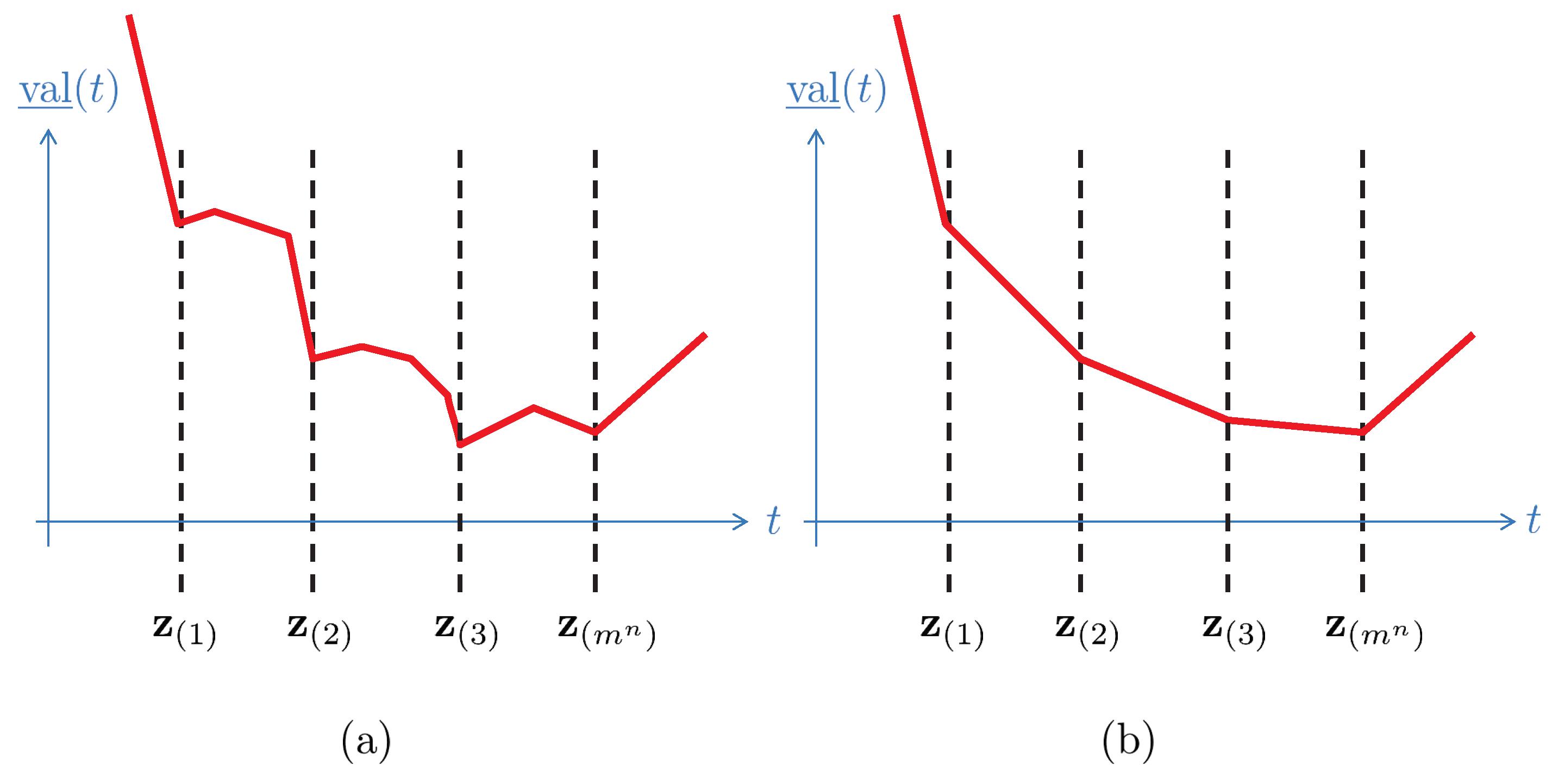
The above proposition, based on classical sensitivity analysis for LP, albeit correct, may be misleading while designing a numerical scheme for minimising $\underset{\_}{\mathrm{val}}\left(t\right)$. Specifically, the asserted piecewise concavity of $\underset{\_}{\mathrm{val}}\left(t\right)$ may suggest a potential existence of several local minima (see Figure 1a). We remedy this in the next theorem, which gives a complete characterisation of the partial value function. Along the way, we drastically reduce the upper bound on the number of linear segments comprising $\underset{\_}{\mathrm{val}}\left(t\right)$.

Theorem 2.

The function $\underset{\_}{\mathrm{v}}\left(t\right)$ is continuous, non-negative and non-increasing, satisfying $\underset{\_}{\mathrm{v}}\left(t\right)=0$ for $t\ge {\mathbf{z}}_{\left(m^n\right)}$ and ${\underset{\_}{\mathrm{v}}}^{\prime }\left(t\right)=-1$ for $t\le {\mathbf{z}}_{\left(1\right)}$. Moreover, $\underset{\_}{\mathrm{v}}\left(t\right)$ is convex on ℜ and linear on every subinterval $[{\mathbf{z}}_{(\ell )},{\mathbf{z}}_{(\ell +1)}]$.

Proof. 

Continuity and the tail-end behaviour of $\underset{\_}{\mathrm{v}}\left(t\right)$ are established in the proof of Proposition 1 and Theorem 1. Examining variational formulation (5), we easily note the non-negativity and monotonicity of the partial value function, with the latter, due to the objective coefficients ${({\mathbf{z}}_{\mathbf{i}}-t)}_{+}$, being monotone in t. Linearity on $[{\mathbf{z}}_{(\ell )},{\mathbf{z}}_{(\ell +1)}]$ follows as a consequence of convexity—to be established shortly—and piecewise concavity in Proposition 1. It remains to show convexity.

We show the convexity property by contradiction. First, introduce

$$\begin{array}{c}\hfill {\displaystyle {\mathrm{v}}_{\mathbf{p}}\left(t\right):=\sum _{\mathcal{I}}{({\mathbf{z}}_{\mathbf{i}}-t)}_{+} {\mathbf{p}}_{\mathbf{i}}}\end{array}$$

to be the partial value function restricted to a given feasible $\mathbf{p}$. Observe that ${\mathrm{v}}_{\mathbf{p}}$ is convex, piecewise linear non-increasing, and its derivative ${\mathrm{v}}_{\mathbf{p}}^{\prime }\left(t\right)$, whenever defined, corresponds to the dot product of $\mathbf{p}$ with the corresponding sub-vector of $\Delta \mathbf{c}$, as in (7). Thus, ${\mathrm{v}}_{\mathbf{p}}^{\prime }\left(t\right)$ is non-decreasing whenever defined. We also note that as t passes from the interval $[{\mathbf{z}}_{(\ell -1)},{\mathbf{z}}_{(\ell )}]$ to $[{\mathbf{z}}_{(\ell )},{\mathbf{z}}_{(\ell +1)}]$, the number of $-1$ entries, i.e., the non-zeros in $\Delta \mathbf{c}$, is reduced by at least one.

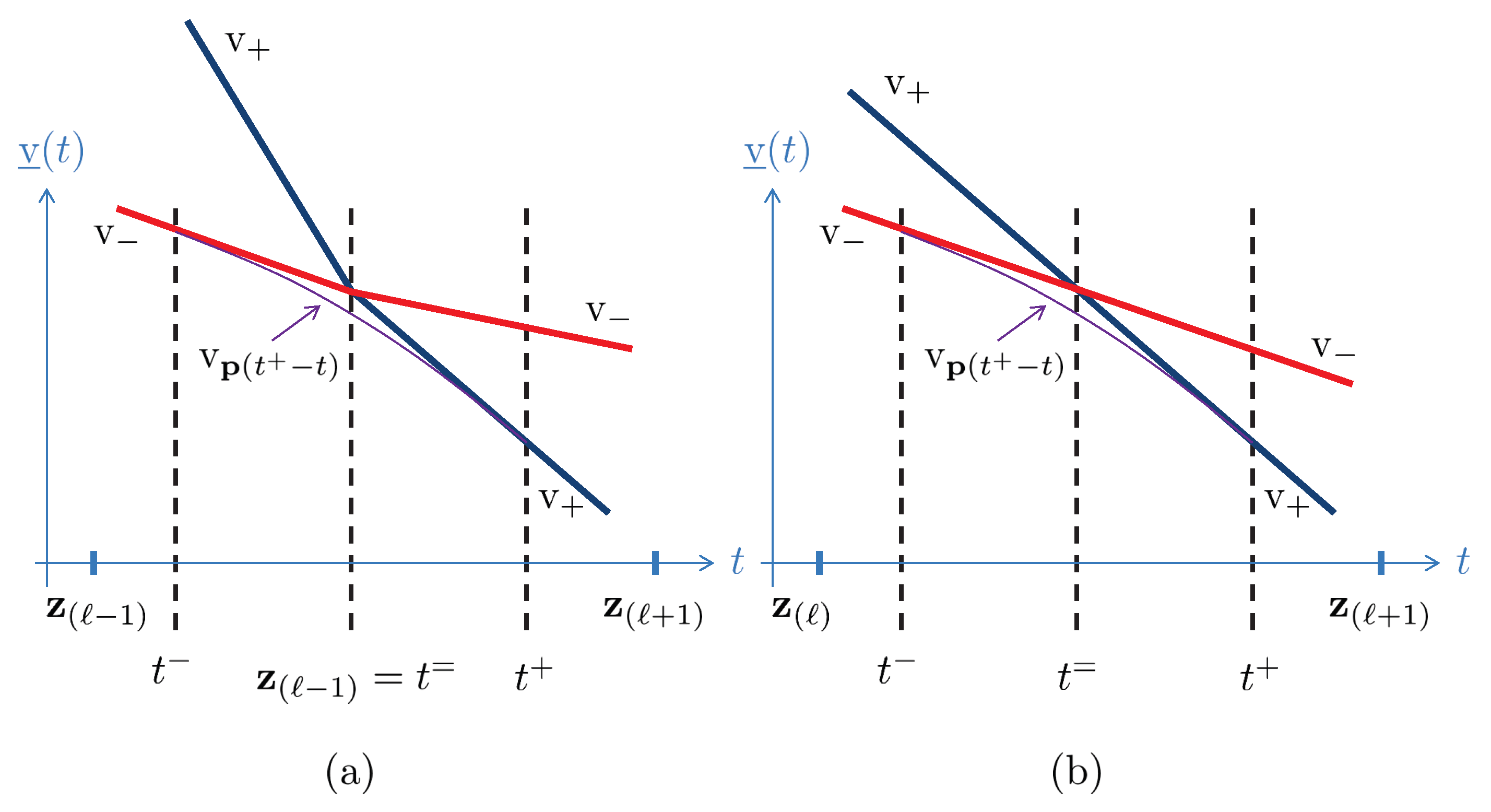
If $\underset{\_}{\mathrm{v}}\left(t\right)$ is strictly concave, there exists a cross-over point $t^{=}$, characterized by $t^{-}<t^{=}<t^{+}$ and the corresponding optimal distributions ${\mathbf{p}}^{-}$ and ${\mathbf{p}}^{+}$, resolving (6) such that ${\mathrm{v}}_{-}\left(t^{=}\right)={\mathrm{v}}_{+}\left(t^{=}\right)$, with derivatives satisfying ${\mathrm{v}}_{-}^{\prime }\left(t^{-}\right)>{\mathrm{v}}_{+}^{\prime }\left(t^{-}\right)$ and ${\mathrm{v}}_{-}^{\prime }\left(t^{+}\right)>{\mathrm{v}}_{+}^{\prime }\left(t^{+}\right)$, where ${\mathrm{v}}_{-}\left(t\right):={\mathrm{v}}_{{\mathbf{p}}^{-}}\left(t\right)$ and ${\mathrm{v}}_{+}\left(t\right):={\mathrm{v}}_{{\mathbf{p}}^{+}}\left(t\right)$. Note that $t^{-}$ and $t^{+}$ may be chosen close enough to $t^{=}$ to warrant differentiability of the corresponding piecewise linear ${\mathrm{v}}_{+},{\mathrm{v}}_{-}$ on $[t^{-},t^{=})$ and $(t^{=},t^{+}]$. Furthermore, without a loss in generality, we may assume that both ${\mathrm{v}}_{-}\left(t\right),{\mathrm{v}}_{+}\left(t\right)$ have either at most one break-point at ${\mathbf{z}}_{(\ell )}=t^{=}$ for some ℓ with $t^{-}\in ({\mathbf{z}}_{(\ell -1)},{\mathbf{z}}_{(\ell )})$ and $t^{+}\in ({\mathbf{z}}_{(\ell )},{\mathbf{z}}_{(\ell +1)})$, or no break-point at all with $t^{-},t^{+}\in ({\mathbf{z}}_{(\ell )},{\mathbf{z}}_{(\ell +1)})$, as can be seen in Figure 2. By re-scaling and shifting t we can also assume $t^{=}\equiv 0$ and $-t^{-}=t^{+}=\frac{1}{2}$. With the above notation, we have $\underset{\_}{\mathrm{v}}\left(t\right)=min\{{\mathrm{v}}_{-}\left(t\right),{\mathrm{v}}_{+}\left(t\right)\}$ for $t\in [-1/2,1/2]$ and ${\mathrm{v}}_{-}^{\prime }\left(t\right)>{\mathrm{v}}_{+}^{\prime }\left(t\right)$ for $t\in [-1/2,0)\bigcup (0,1/2]$.

Denote $\mathbf{p}\left(\tau \right)=\tau {\mathbf{p}}^{-}+(1-\tau ){\mathbf{p}}^{+}, \tau \in [0,1]$. Note that $\mathbf{p}\left(\tau \right)$ is feasible since the feasible region of (6) is convex. Further, let us examine $v\left(\tau \right):={\mathrm{v}}_{\mathbf{p}\left(\tau \right)}(1/2-\tau )$. By the fundamental theorem of calculus, we obtain

$$\begin{array}{c}\hfill {\displaystyle v(1/2)=v\left(0\right)+{\int }_0^{1/2}{v}_{\tau }^{\prime }\left(\tau \right) d\tau =\underset{\_}{\mathrm{v}}\left(t^{+}\right)+{\int }_0^{1/2}{\mathrm{v}}_{\mathbf{p}\left(\tau \right)}^{\prime }\left(\tau \right) d\tau <\underset{\_}{\mathrm{v}}\left(t^{=}\right),}\end{array}$$

where the inequality is due to the fact that $\left|{\mathrm{v}}_{\mathbf{p}\left(\tau \right)}^{\prime }\left(\tau \right)\right|<\left|{\mathrm{v}}_{+}^{\prime }\left(\tau \right)\right|$, for all $\tau \in (0,1/2)$, since ${\mathbf{p}}^{-}$; consequently, $\mathbf{p}\left(\tau \right)$ carries less probability mass over the support of $\Delta \mathbf{c}$ at $t^{+}$ as compared to ${\mathbf{p}}^{+}$. Since $\underset{\_}{\mathrm{v}}\left(t^{=}\right)$ is supposed to be the smallest over all feasible $\mathbf{p}$ at $t^{=}$, the contradiction is conspicuous. This completes the proof.  □

3.4. Two Computational Approaches

We now present two computational schemes for computing the sharp lower bound ${\underset{\_}{\mathrm{CVaR}}}_{\alpha }$ on CVaR given the constraints on the risks’ c.d.f.. The schemes are aimed at illustrating the advantages of exploiting the inherent structure of Problem 3 and range in order of complexity, as well as the perceived numerical efficiency. The latter is further substantiated in Section 5.

3.4.1. Naïve Scheme

Observe that the piecewise concavity of $\underset{\_}{\mathrm{val}}\left(t\right)$ established in Proposition 1 implies that the minimum of the value function may only occur at the end points of each interval $[{\mathbf{z}}_{(\ell )},{\mathbf{z}}_{(\ell +1)}]$. Therefore, it suffices to compute $\underset{\_}{\mathrm{val}}\left({\mathbf{z}}_{\mathbf{i}}\right)$ for all $\mathbf{i}$ and take the minimum value. This gives rise to the naïve scheme.

Clearly, the naïve scheme requires access to an LP solver and runs in finite time. However, it requires solving a large number—namely $m^n$—of (6)-type optimization problems, where the problem dimensions also grow proportional to $m^n$. As a result, the procedure may become very computationally expensive for even modest values of m and n. Further effort can be put towards reducing the computational requirements imposed by the naïve scheme. For example, the LP problems for evaluating $\underset{\_}{\mathrm{val}}\left(t\right)$ differ only in the objective function, and thus, may be well-suited for the so-called warm-start techniques, as in simplex-type algorithms. In turn, the use of warm-starting may speed up solution times.

3.4.2. Epigraph Scheme

Unlike the naïve scheme, here we aim to take full advantage of the uncovered convexity of the value function. This not only allows us to greatly reduce the computational efforts required to determine the exact value ${\underset{\_}{\mathrm{CVaR}}}_{\alpha }$, but also permits the introduction of an alternative termination criterion when only an approximate answer is required within some given absolute precision $\epsilon >0$.

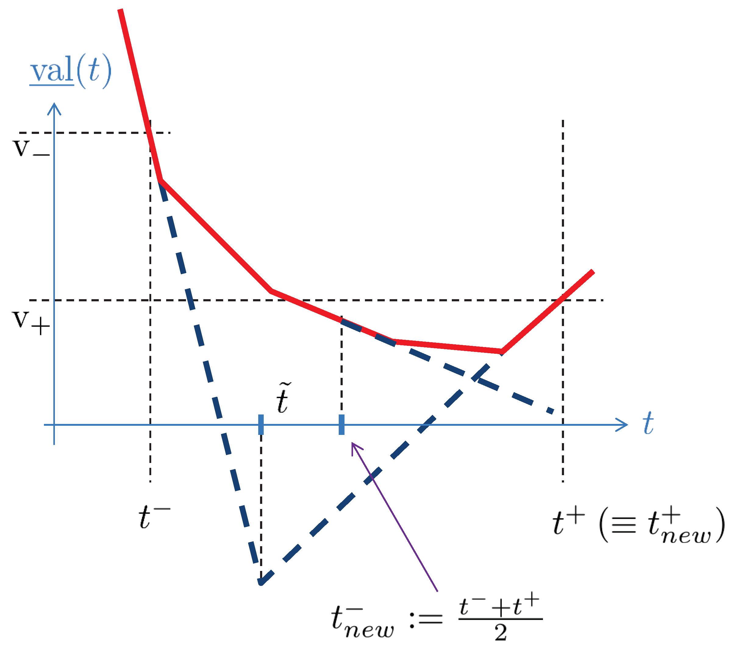
We recall that an epigraph of a convex function can be obtained as an intersection of half-spaces. In the case of a smooth function the half-spaces correspond to tangent hyperplanes, and in the case of non-differentiable functions one may use half-spaces defined by sub-gradients. Thus, given two consecutive values $t^{-}<t^{+}$ of t with appropriately defined derivatives ${\underset{\_}{\mathrm{val}}}^{\prime }\left(t\right)$ of $\underset{\_}{\mathrm{val}}\left(t\right)$, with values ${\mathrm{v}}_{-}:=\underset{\_}{\mathrm{val}}\left(t^{-}\right),{\mathrm{v}}_{+}:=\underset{\_}{\mathrm{val}}\left(t^{+}\right)$ and ${\mathrm{v}}_{-}^{\prime }:={\underset{\_}{\mathrm{val}}}^{\prime }\left(t^{-}\right)<0,{\mathrm{v}}_{+}^{\prime }:={\underset{\_}{\mathrm{val}}}^{\prime }\left(t^{+}\right)>0$, we know that the minimal value ${\underset{\_}{\mathrm{val}}}^{*}$ of $\underset{\_}{\mathrm{val}}\left(t\right)$ corresponds to some $t^{*}\in [t^{-},t^{+}]$. In addition, we have ${\underset{\_}{\mathrm{val}}}^{*}\in [min({\mathrm{v}}_{-},{\mathrm{v}}_{+}),\underset{\_}{\mathrm{val}}\left(\tilde{t}\right)]$, where

$$\tilde{t}=\frac{{\mathrm{v}}_{-}-{\mathrm{v}}_{+}+{\mathrm{v}}_{+}^{\prime }{t}^{+}-{\mathrm{v}}_{-}^{\prime }{t}^{-}}{{\mathrm{v}}_{+}^{\prime }-{\mathrm{v}}_{-}^{\prime }}$$

is the intersection of the supporting hyperplanes ${\mathrm{v}}_{-}^{\prime } (t-t^{-})+{\mathrm{v}}_{-}$ and ${\mathrm{v}}_{+}^{\prime } (t-t^{+})+{\mathrm{v}}_{+}$. This can be seen in Figure 3. To refine the interval $[t^{-},t^{+}]$ and our estimate on ${\underset{\_}{\mathrm{val}}}^{*}$, we can take the mid-point of the interval and adjust either $t^{-},{\mathrm{v}}_{-},{\mathrm{v}}_{-}^{\prime }$ or $t^{+},{\mathrm{v}}_{+},{\mathrm{v}}_{+}^{\prime }$ accordingly.

Assuming that the data are given by $\alpha ,m,n,\underset{\_}{\mathbf{ß}},\overline{\mathbf{ß}}$, and $\mathbf{z}$, the scheme may be defined recursively as a function whose declaration is given below using MATLAB notation

$$\mathtt{function} \mathtt{[}{\displaystyle t^{-},t^{+},{\mathrm{v}}_{-},{\mathrm{v}}_{+},{\mathrm{v}}_{-}^{\prime },{\mathrm{v}}_{+}^{\prime }\mathtt{]}\mathtt{=}\mathtt{Epigraph}\mathtt{(}{t}^{-},t^{+},{\mathrm{v}}_{-},{\mathrm{v}}_{+},{\mathrm{v}}_{-}^{\prime },{\mathrm{v}}_{+}^{\prime }\mathtt{)}\mathtt{,}}$$

and is defined as follows.

• [Input:] $t^{-}<t^{+},{\mathrm{v}}_{-}^{\prime }\le 0,{\mathrm{v}}_{+}^{\prime }\ge 0,{\mathrm{v}}_{-},{\mathrm{v}}_{+}$, problem data.
• Set ${\underset{\_}{\mathrm{val}}}^{*}:=min\{{\mathrm{v}}_{-},{\mathrm{v}}_{+}\}$,
• compute $\tilde{t}$ and $\mathrm{v}:=\underset{\_}{\mathrm{val}}\left(\tilde{t}\right)$ by solving (5), recovering the optimal probability distribution $\tilde{\mathbf{p}}$,
• if $\mathrm{v}={\underset{\_}{\mathrm{val}}}^{*}$ then return,
• set ${\displaystyle {\mathrm{v}}^{\prime }:=1+\frac{1}{1-\alpha } \sum _{\mathcal{I}}\Delta {\mathbf{c}}_{\mathbf{i}} {\tilde{\mathbf{p}}}_{\mathbf{i}}}$ with $\Delta \mathbf{c}$ corresponding to $\tilde{t}$ as in (7),
• if ${\mathrm{v}}^{\prime }\le 0$ set $t^{-}:=\tilde{t},{\mathrm{v}}_{-}:=\mathrm{v},{\mathrm{v}}_{-}^{\prime }:={\mathrm{v}}^{\prime }$,
• if ${\mathrm{v}}^{\prime }>0$ set $t^{+}:=\tilde{t},{\mathrm{v}}_{+}:=\mathrm{v},{\mathrm{v}}_{+}^{\prime }:={\mathrm{v}}^{\prime }$,
• invoke Epigraph($t^{-},t^{+},{\mathrm{v}}_{-},{\mathrm{v}}_{+},{\mathrm{v}}_{-}^{\prime },{\mathrm{v}}_{+}^{\prime }$).
• [Output:] ${\displaystyle {\underset{\_}{\mathrm{val}}}^{*}=\underset{t\in [t^{-},t^{+}]}{min}\underset{\_}{\mathrm{val}}\left(t\right)}$.

Clearly, in order to obtain ${\underset{\_}{\mathrm{CVaR}}}_{\alpha }$, we need to invoke Epigraph($t^{-},t^{+},{\mathrm{v}}_{-},{\mathrm{v}}_{+},{\mathrm{v}}_{-}^{\prime },{\mathrm{v}}_{+}^{\prime }$) with initial values $t^{-}=\underset{\_}{t} (\equiv {\mathbf{z}}_{\left(1\right)})$ and $t^{+}=\overline{t} (\equiv {\mathbf{z}}_{\left(m^n\right)})$. If one desires to terminate the procedure once the absolute precision $\epsilon$ is reached, such that ${\underset{\_}{\mathrm{val}}}^{*}\le {\underset{\_}{\mathrm{CVaR}}}_{\alpha }\le {\underset{\_}{\mathrm{val}}}^{*}+\epsilon$, it suffices to replace the function termination criteria $\underset{\_}{\mathrm{val}}-\mathrm{v}=0$ with $min\{-{\mathrm{v}}_{-}^{\prime }(\tilde{t}-t^{-}),{\mathrm{v}}_{+}(t^{+}-\tilde{t})\}\le \epsilon$.

For the convexity of $\underset{\_}{\mathrm{val}}\left(t\right)$ and its tail behaviour from Theorem 2, we know that the fastest decrease rate of the value function does not exceed $\left|1-\frac{1}{1-\alpha }\right|=\frac{\alpha }{1-\alpha }$ and therefore,

$$|\underset{\_}{\mathrm{val}}\left(t\right)-\underset{\_}{\mathrm{val}}(t+\Delta t)|\le \frac{\alpha \Delta t}{1-\alpha }, \mathrm{for} \mathrm{all} t,\Delta t.$$

Thus, in order to achieve an $\epsilon$ precision, it suffices to have $t^{+}-t^{-}\le \frac{\epsilon (1-\alpha )}{\alpha }$. In turn, recalling that at every iteration of the scheme the interval $[t^{-},t^{+}]$ is halved, we conclude that the absolute $\epsilon$ precision can be attained in at most ${log}_2\left(\frac{1}{\epsilon }·\frac{\alpha (\overline{t}-\underset{\_}{t})}{(1-\alpha )}\right)$ recursive calls, where the dominant work belongs to solving an LP instance of the form (6).

In a nutshell, although the epigraph scheme still relies on solving multiple LP instances in order to recover ${\underset{\_}{\mathrm{CVaR}}}_{\alpha }$ for fixed n, its worst-case run-time is bounded from above as a polynomial function of the problem input. Furthermore, when an approximate solution is sufficient, one would expect the number of calls to the LP solver to be dramatically less than $m^n$, as compared to the naïve scheme. We also note that the epigraph procedure is defined recursively only in an attempt to improve clarity of exposition. Clearly, the procedure can be unrolled into if ... else ... statements with no recursion. Just as with the naïve scheme, one may try to take advantage of the warm-starting capabilities of an LP solver in an attempt to speed up the computational times required.

4. Computable Upper Bound

It turns out that despite apparent similarities between Problems (3) and (4), the complexity of evaluating ${\underset{\_}{\mathrm{CVaR}}}_{\alpha }$ is quite different from that of ${\overline{\mathrm{CVaR}}}_{\alpha }$. Namely, the calculation of ${\overline{\mathrm{CVaR}}}_{\alpha }$ is much simpler. We first establish an essential property that is needed for proving the main result of this section.

Proposition 2.

The max-value function $\overline{\mathrm{val}}\left(t\right)=t+\frac{1}{1-\alpha } \overline{\mathrm{v}}\left(t\right)$, where

$$\begin{array}{c}\hfill \begin{array}{cc}\overline{\mathrm{v}}\left(t\right):=\hfill & {\displaystyle \underset{\mathbf{p}}{max}\sum _{\mathcal{I}}{({\mathbf{z}}_{\mathbf{i}}-t)}_{+} {\mathbf{p}}_{\mathbf{i}}}\hfill \\ \mathrm{s}.\mathrm{t}.\hfill & {\displaystyle {\underset{\_}{\mathbf{ß}}}_{\mathbf{i}}\le \sum _{\mathbf{j}\le \mathbf{i}}{\mathbf{p}}_{\mathbf{j}}\le {\overline{\mathbf{ß}}}_{\mathbf{i}}, \mathrm{for} \mathrm{all} \mathbf{i}\in \mathcal{I},}\hfill \\ & {\displaystyle \sum _{\mathbf{i}: i_j=k}{\mathbf{p}}_{\mathbf{i}}=\frac{1}{m}, \mathrm{for} \mathrm{all} j=1,\dots ,n, k=1,\dots ,m,}\hfill \\ & {\displaystyle \sum _{\mathcal{I}}{\mathbf{p}}_{\mathbf{i}}=1, \mathbf{p}\ge 0,}\hfill \end{array}\end{array}$$

is convex in t.

Proof. 

For fixed non-negative $\mathbf{p}$, the objective function ${\sum }_{\mathcal{I}}{({\mathbf{z}}_{\mathbf{i}}-t)}_{+} {\mathbf{p}}_{\mathbf{i}}$ is convex in t. In turn, $\overline{\mathrm{v}}\left(t\right)$ is obtained by taking a supremum of convex functions ${\mathrm{v}}_{\mathbf{p}}\left(t\right)$, indexed by $\mathbf{p}$, and therefore $\overline{\mathrm{val}}\left(t\right)$ is convex as well as a positive weighted sum of t and $\overline{\mathrm{v}}\left(t\right)$.  □

Using convexity, we note that the epigraph-based scheme from Section 3.4.2 can readily be adapted to computing the sharp upper bound of ${\mathrm{CVaR}}_{\alpha }$. Furthermore, using classical LP duality theory, finding the optimal t value corresponding to minimising $\overline{\mathrm{val}}\left(t\right)$ may equivalently be reformulated as solving a linear optimization problem. Let

$$\begin{array}{c}\hfill {\mathcal{M}}_{j,k}=\{\mathbf{i}: i_j=k,i_{\ell }=m \mathrm{for} \mathrm{all} \ell \ne j\}\end{array}$$

(8)

and ${\displaystyle \mathcal{M}=\bigcup _{j,k}{\mathcal{M}}_{j,k}}$ denote the set of multi-indices corresponding to sums of marginals, including the total probability mass. For simplicity, from now on, we assume that the c.d.f. bounds $\overline{\mathbf{ß}},\underset{\_}{\mathbf{ß}}$ are consistent with marginals, that is, ${\underset{\_}{\mathbf{ß}}}_{\mathbf{i}}\le \frac{k}{m}\le {\overline{\mathbf{ß}}}_{\mathbf{i}}$ for all $\mathbf{i}\in {\mathcal{M}}_{j,k}$ where the marginal index sets are defined as in (8). If not, clearly, the problem of computing $\overline{\mathrm{val}}\left(t\right)$ is infeasible.

For clarity of exposition, we first slightly modify our formulation of $\overline{\mathrm{v}}\left(t\right)$ from above. Noting that the lower and upper bound requirements on the c.d.f. are clearly redundant for $\mathbf{i}\in \mathcal{M}$, they may simply be replaced with more restrictive modified bounds ${\underset{\_}{\mathbf{ß}}}^{\prime },{\overline{\mathbf{ß}}}^{\prime }$, where

$${\underset{\_}{\mathbf{ß}}}_{\mathbf{i}}^{\prime }=\left\{\begin{array}{cc}\frac{k}{m},\hfill & \mathbf{i}\in {\mathcal{M}}_{j,k},\forall j,k,\hfill \\ {\underset{\_}{\mathbf{ß}}}_{\mathbf{i}},\hfill & \mathrm{otherwise},\hfill \end{array}\right.\hspace{1em}\mathrm{and}\hspace{1em}{\overline{\mathbf{ß}}}_{\mathbf{i}}^{\prime }=\left\{\begin{array}{cc}\frac{k}{m},\hfill & \mathbf{i}\in {\mathcal{M}}_{j,k},\forall j,k,\hfill \\ {\overline{\mathbf{ß}}}_{\mathbf{i}},\hfill & \mathrm{otherwise}.\hfill \end{array}\right.$$

We are now ready to formulate the main result of this section.

Theorem 3.

The upper bound defined in (4) can be computed as follows:

$$\begin{array}{c}\hfill \begin{array}{cc}{\overline{\mathrm{CVaR}}}_{\alpha }:=\hfill & {\displaystyle \underset{t,\underset{\_}{\mathbf{y}},\overline{\mathbf{y}}}{min}t+\frac{1}{1-\alpha }\left(-{\underset{\_}{\mathbf{y}}}^T{\underset{\_}{\mathbf{ß}}}^{\prime }+{\overline{\mathbf{y}}}^T{\overline{\mathbf{ß}}}^{\prime }\right)}\hfill \\ \mathrm{s}.\mathrm{t}.\hfill & {\displaystyle \sum _{\mathbf{j}\ge \mathbf{i}}{\underset{\_}{\mathbf{y}}}_{\mathbf{j}}-\sum _{\mathbf{j}\ge \mathbf{i}}{\overline{\mathbf{y}}}_{\mathbf{j}}\le t-{\mathbf{z}}_{\mathbf{i}}, \mathrm{for} \mathrm{all} \mathbf{i}\in \mathcal{I},}\hfill \\ & {\displaystyle \sum _{\mathbf{j}\ge \mathbf{i}}{\underset{\_}{\mathbf{y}}}_{\mathbf{j}}-\sum _{\mathbf{j}\ge \mathbf{i}}{\overline{\mathbf{y}}}_{\mathbf{j}}\le 0, \mathrm{for} \mathrm{all} \mathbf{i}\in \mathcal{I},}\hfill \\ & {\displaystyle \underset{\_}{\mathbf{y}},\overline{\mathbf{y}}\ge 0, t\in \Re ,}\hfill \end{array}\end{array}$$

Proof. 

Note that for any fixed t, the problem of computing $\overline{\mathrm{v}}\left(t\right)$ is equivalent to solving its dual

$$\begin{array}{c}\hfill \begin{array}{cc}{\overline{\mathrm{v}}}^{*}\left(t\right):=\hfill & {\displaystyle \underset{\underset{\_}{\mathbf{y}},\overline{\mathbf{y}}}{min}-{\underset{\_}{\mathbf{y}}}^T{\underset{\_}{\mathbf{ß}}}^{\prime }+{\overline{\mathbf{y}}}^T{\overline{\mathbf{ß}}}^{\prime }}\hfill \\ \mathrm{s}.\mathrm{t}.\hfill & {\displaystyle \sum _{\mathbf{j}\ge \mathbf{i}}{\underset{\_}{\mathbf{y}}}_{\mathbf{j}}-\sum _{\mathbf{j}\ge \mathbf{i}}{\overline{\mathbf{y}}}_{\mathbf{j}}\le -{({\mathbf{z}}_{\mathbf{i}}-t)}_{+}, \mathrm{for} \mathrm{all} \mathbf{i}\in \mathcal{I},}\hfill \\ & {\displaystyle \underset{\_}{\mathbf{y}},\overline{\mathbf{y}}\ge 0,}\hfill \end{array}\end{array}$$

where by strong LP duality, we know that ${\overline{\mathrm{v}}}^{*}\left(t\right)=\overline{\mathrm{v}}\left(t\right)$. Furthermore, for any dual-feasible point $(\underset{\_}{\mathbf{y}},\overline{\mathbf{y}})$, by the weak duality property we have $-{\underset{\_}{\mathbf{y}}}^T{\underset{\_}{\mathbf{ß}}}^{\prime }+{\overline{\mathbf{y}}}^T{\overline{\mathbf{ß}}}^{\prime }\ge \overline{\mathrm{v}}\left(t\right).$

Noting that the dual-feasible region may equivalently be rewritten as stated in the theorem, we finally observe that in order to compute the optimal $t^{*}$ that satisfies ${\overline{\mathrm{CVaR}}}_{\alpha }=\overline{\mathrm{val}}\left(t^{*}\right)$, it suffices to solve the concurrent linear minimisation problem with respect to t and $(\underset{\_}{\mathbf{y}},\overline{\mathbf{y}})$.  □

Finally, once the optimal value $t^{*}$ is known, the corresponding optimal values of $\mathbf{p}$ can easily be computed by solving for $\overline{\mathrm{v}}\left(t^{*}\right)$ as a linear maximisation problem, if further desired.

5. Numerical Results

In this section, we provide numerical illustrations of our findings from Section 3 and Section 4. First, we gauge how the computational requirements scale up with the problem dimensions and identify one critical bottleneck in Section 5.1. To do this, we compare two ways of implementing our approaches in MATLAB. One primarily relies on CVX with the embedded open-source solver SDPT3, chosen for the sake of simplicity. The other approach uses Gurobi Optimization, LLC (2023) and a direct problem formulation, as a potentially more efficient option. CVX removes the inconvenience of carefully formulating the LP (6) to near-standard form suitable for Gurobi, while potentially sacrificing some of the efficiencies. On the other hand, the user-provided direct specification of the underlying LP may be more of a challenge initially, but potentially gives some computational advantage when solving the problem. Next, we propose an approach that allows us to circumvent one of the main computational obstacles, and illustrate the refined methodology on a real-life inspired example in Section 5.2.

5.1. Verbatim Implementation

Our first goal is to obtain a sense of how the performance of our method scales up with problem dimensions, as well as to gauge if the modeling environment and the LP solver play a role. For this, we use a very modest Alienware laptop with a 2 core Intel i7 U640 CPU running at 1.2 GHz, 4 GB RAM, running Windows 7 x64, MATLAB R2013b, CVX 2.0, and Gurobi 5.5.

Regardless of the approach, we rely on solving (5) or its variant, where the dimensions of the problem grow proportional to $m^n$—thus, polynomial in m and exponential in n. Specifically, for the standard LP form of the partial value evaluation (6), the number of variables and constraints grow as $3m^n$ and $2m^n+mn+1$, respectively, while the number of non-zeros in the matrix of coefficients describing the affine constraint is roughly $2m^{2n}·{\left(\frac{m+1}{2m}\right)}^n$.2 Consequently, despite the fact that the fraction of non-zero entries in the matrix of affine coefficients corresponding to (6) decreases exponentially in n, the number of non-zeros still grows very rapidly with the number of risks. For instance, in case of $m=100$ and $n=3$, one should expect to deal with a matrix containing more than ${10}^{11}$ non-zero entries (of one), making solving such problems on a regular computer workstation prohibitively expensive. Even with the availability of super-computing resources, one probably has to resort to very specialized algorithms—e.g., Tardos (1986)—and linear algebra techniques to exploit matrix sparsity structure efficiently for large values of m and n.

In

Table 1. Average run-time (in seconds) for naïve and epigraph schemes for small size problems with $\epsilon ={10}^{-10}$.

			SDPT3					Gurobi
		Naïve		Epigraph		Naïve			Epigraph
n	m	CVX	CVX+	CVX	CVX+	CVX	CVX+	Direct	CVX	CVX+	Direct
2	2	2.59	2.53	6.71	6.77	1.41	1.38	0.10	6.80	6.66	0.27
	4	9.26	8.38	17.04	16.16	4.06	3.80	0.19	8.01	7.52	0.33
	6	21.85	18.49	18.79	16.85	8.76	8.03	0.36	8.28	7.40	0.38
	8	42.94	35.09	20.75	17.76	16.13	13.97	0.84	8.51	7.41	0.50
	10	77.72	61.51	22.35	18.25	26.60	22.32	1.76	9.20	7.70	0.73
	12	149.49	117.61	29.06	25.27	41.82	33.68	3.57	9.95	8.17	1.11
	14	264.68	200.38	35.92	31.02	63.71	49.53	7.29	10.59	8.40	1.66
3	3	16.05	13.67	19.68	17.10	6.51	6.11	0.29	8.04	7.59	0.37
	4	42.80	35.11	22.57	18.86	15.36	14.05	0.83	8.46	7.70	0.53
	5	109.92	87.24	27.32	22.98	32.05	28.60	2.57	9.18	8.23	0.95
	6	299.76	224.36	39.94	33.52	61.86	53.93	8.40	10.06	8.90	1.91

we report the average run-times for estimating sharp upper and lower bounds for problems with varying n and m. For this and the other numerical experiments, for each dimension, we generate 30 random problem instances, where $X_i$ sample values are chosen to be uniform between 0 and 1 for simplicity. CVX refers to only using CVX to formulate the LP sub-problem and passes it to a selected solver, while tensor-like notation is used inside the CVX code. CVX+ refers to us formulating the affine constraints of an LP in vectorized form and letting CVX only pass the data to the solver. Direct refers to us both formulating the problem and invoking the Gurobi solver directly, bypassing CVX. When not specified, $\alpha =0.95$ and $\epsilon ={10}^{-7}$.

Our first goal is to understand how the proposed methods scale with dimensions. As expected, the computational cost escalates very rapidly when dimensions m, and especially n, increase. We observe that the run-time heavily depends on the LP solver. For Gurobi, here we used the simplex option, while experimenting with the barrier gave inferior results on this dataset; we suspect that the latter can be attributed to being able to take advantage of a simplex warm-start. Even when no top-of-the-line commercial solver is available, one can compute some bounds with $n<3$ in reasonable time for small values of m.

We also note that, in general using CVX, as opposed to directly formulating the problem and feeding it into a solver, poses some processing time overhead, especially for smaller problems. While formulating the matrix of affine constraints, we rely on MATLAB loops, which may potentially be sped up. Solving with $n=2$ and $m=50$ to within an $\epsilon ={10}^{-7}$ precision by using the epigraph scheme, MATLAB takes about 100 s to form a single LP matrix of the coefficients in the standard form, while solving all the subsequent LP problems takes roughly another 150 s.

For estimating the lower bound on ${\mathrm{CVaR}}_{\alpha }$, between the two schemes, the epigraph-based method is a clear winner over the naïve approach. The solution times grow with n and m (see Table 1 and

Table 2. Average run-time (in seconds) for the best lower bound estimation scheme—epigraph-based with direct Gurobi—for small to medium size problems with $\epsilon ={10}^{-7}$, with a run-time limit of 15 min.

$\mathit{n}\setminus \mathit{m}$	3	6	9	12	15	20	30	40	50	60
2	0.24	0.30	0.48	0.91	1.71	4.76	28.08	93.44	240.52	543.52
3	0.29	1.62	16.87	114.93	600.53	-	-	-	-	-

), as well as the desired precision $\epsilon$ (see

Table 3. Average run-time (in seconds) for Gurobi-based epigraph scheme with respect to (a) $\alpha$, with $\epsilon ={10}^{-5}$, and (b) $\epsilon$.

			(a)					(b)
$\mathit{n}$	$\mathit{m}\mathbf{\setminus }\mathbf{\alpha }$	0.1	0.9	0.99	$\mathit{n}$	$\mathit{m}\mathbf{\setminus }\mathbf{ϵ}$	${\mathbf{10}}^{\mathbf{-}\mathbf{3}}$	${\mathbf{10}}^{\mathbf{-}\mathbf{5}}$	${\mathbf{10}}^{\mathbf{-}\mathbf{7}}$
2	20	3.47	3.93	4.21	2	20	3.47	3.96	4.56
	30	20.36	23.36	25.61		30	19.24	22.29	27.53
	40	68.34	74.08	85.97		40	64.46	79.07	92.04
3	6	1.16	1.37	1.46	3	6	1.16	1.35	1.62
	9	11.83	13.90	14.47		9	12.22	14.14	16.84
	12	77.88	95.16	100.65		12	81.13	96.21	122.45

b). By comparing the results in Table 2 and

Table 4. Average run-time (in seconds) for the upper bound using Gurobi-based epigraph and direct LP embedding methods, with $\epsilon ={10}^{-10}$, with a run-time limit of 15 min.

Method	$\mathit{n}\mathbf{\setminus }\mathit{m}$	3	6	9	12	20	30	40	50	60
Epigraph	2	0.32	0.35	0.60	1.14	5.88	35.60	139.0	354.4	688.6
Direct LP		0.05	0.07	0.13	0.33	2.64	12.05	39.2	98.4	218.1
Epigraph	3	1.94	21.7	172.5	802.2	-	-	-	-	-
Direct LP		0.67	7.41	44.6	190.9	-	-	-	-	-

, we conclude that computing the sharp upper bound is generally cheaper, as compared to the lower bound. When computing an exact sharp upper bound, direct LP embedding is preferred.

5.2. Stylized Practice-Inspired Example

Computing CVaR sharp bounds under given marginals and lower-orthant stochastic ordering bounds on joint c.d.f.’s, and in particular sharp lower bound, entails solving a non-convex (bilinear) optimization problem of potentially very high dimensionality. Namely, we seek to determine the extreme values of $m^n$ variables representing the c.d.f. When attempting to scale up the model sizes n and m, we are faced with an obvious memory requirement issue. For instance, solving for $n=3, m=100$ in (3) entails formulating a model with over ${10}^{11}$ non-zeros that requires almost 1000 GB of RAM if we operate in standard double-precision arithmetic. The RAM requirement grows as $m^{2n}$ and it is reasonable to expect a significant growth in the computational effort required to solve the model as well.

However, it turns out that one could produce a much sparser equivalent representation of lower and upper bound optimization models, allowing solving for sharp bounds with $n=3, m=100$ sized models in a reasonable time, i.e., a couple of hours, on a reasonable hardware, i.e., a multi-core station with enough RAM. Next, we present this refined setup, along with a more practical illustration of our approach. The example is partly based on work carried out outside of this manuscript, and has been further stylized to avoid breaching any possible non-disclosure agreements. We focus on the lower bound computation as it is more challenging; the upper bound evaluation can be refined in a similar manner.

Assume an insurance company with a portfolio of three risks, located in (1) New York (NY), (2) Miami (FL) and (3) Houston (TX), for which the policy covers economic damages to certain buildings caused by hurricanes in these regions. The underwriter makes decisions based on the hurricane intensity estimates that in turn are predicted based on an atmospheric internal risk model. If $X_k$ with $k\in \{1,2,3\}$ is the economic damage for the k-th risk in dollars, we know that $X_k$ is $\mathrm{Pareto}({\alpha }_k,{\lambda }_k)$, so that the c.d.f. along with the first two moments are

$$F\left(x\right)=1-{\left(\frac{\lambda }{x+\lambda }\right)}^{\alpha }, x\ge 0, \mathrm{E}X=\frac{\lambda }{\alpha -1}, \mathrm{Var}X=\frac{\alpha {\lambda }^2}{(\alpha -2){(\alpha -1)}^2},$$

with

$${\alpha }_1=5, {\alpha }_2=2.1, {\alpha }_3=2.7, {\lambda }_1=7.92\times {10}^6, {\lambda }_2=1.11\times {10}^7, {\lambda }_3=7.36\times {10}^6$$

resulting in expected losses of USD 1.98 million, USD 10.07 million and USD 4.33 million, respectively. Further, for each risk, the coefficient of variation (CV), a well-known measure of risk, is 1.29, 4.58, and 1.96, so indeed the assets are risky, as expected. A large CV is expected for coverage in more risky regions.

The underwriter has empirical evidence (based on atmospheric observational data) to identify the marginal risk distributions, but does not have the knowledge to create a spatial dependence model across the risks located in different regions. Geographical-dependent ratings would be hardily available even to world-leading rating agencies. Therefore, the underwriter has to rely on the available domain knowledge to come up with aggregate risk estimates ${\mathrm{CVaR}}_{\alpha }(X_1+X_2+X_3)$ based on the best possible information about the risk position.

It is clear that $X_k$’s are not negatively associated, and thus, a lower bound on the joint distribution, in terms of the lower-orthant (LO) stochastic ordering, can be given by the independence model,

$$\underset{\_}{\mathrm{F}}(x_1,x_2,x_3)=F_1\left(x_1\right)F_2\left(x_2\right)F_3\left(x_3\right),$$

where $F_k$ is the c.d.f. of $X_k, k=1,2,3$. The upper bound on the joint distribution, in terms of LO, assumes that the NY economic damages are independent of the other two, while economic damages from Miami and Houston could be strongly positive dependent, i.e., comonotonic, and therefore

$$\overline{\mathrm{F}}(x_1,x_2,x_3)=F_1\left(x_1\right)min(F_2\left(x_2\right),F_3\left(x_3\right)).$$

In terms of our CVaR lower bound formulation (3), the above can be encoded via discretizing the individual risks with some fixed m, so that $x_{i,1}\le \dots \le x_{i,m}, i=1,2,3$ correspond to Pareto distribution sample values or inverse Pareto-c.d.f.’s at mid-points $j=(j-1/2)/m$, with

$${\underset{\_}{\mathbf{ß}}}_{i_1,i_2,i_3}=\frac{i_1}{m}\times \frac{i_2}{m}\times \frac{i_3}{m}, {\overline{\mathbf{ß}}}_{i_1,i_2,i_3}=\frac{i_1}{m}\times max\left(\frac{i_2}{m},\frac{i_3}{m}\right).$$

Our objective here is to evaluate the lower bound, specifically, ${\underset{\_}{\mathrm{CVaR}}}_{.8}$ for $n=3, m=100$.

Using a sparse reformulation of (3), which we discuss next, this objective indeed can be achieved in a reasonable computation time, here, in about 2 h, or 7554 s to be precise, yielding ${\underset{\_}{\mathrm{CVaR}}}_{.8}=40.6$ mn, corresponding to $t^{*}=20,914,036$, with the bound computed to within the relative precision of $2.5\times {10}^{-7}$. For this set of computational experiments we move to a more powerful machine, with an AMD EPYC 7313P 16-core processor and 256 GB RAM, running Ubuntu 22.04. To solve the subsequent LPs, we use Gurobi 10.0.1, where the model was implemented using Gurobi’s Python API, and benchmarked using Python 3.7. We want to emphasize that the chief enabling factor is the sparse reformulation that reduces the number of non-zeros in the model by a square root, e.g., going from ${10}^{11}$ to about ${10}^6$ for $n=3, m=100$, allowing the formulation of the model in RAM as well as permitting vastly faster computations, which is further improved by moving to a powerful computer server. The code can be found on GitHub, as per Zinchenko (2023).

A number of further computational experiments were performed with varying sparsified model dimensions for both n and m and the run-times were recorded. A model with $n=3, m=50$ could now be solved in about 550 s, while $n=3, m=150$ is the current computational limit for the above machine. The solve time scales super-linearly with the problem dimensions. For lower dimensional models with $n=2$, as before, the run-times look more favourable; for instance $n=2, m=1000$ could be solved in 808 s.

The sparse reformulation of (3) is built on a pivotal observation that joint c.d.f.’s can be defined recursively, using inclusion–exclusion formulas. Namely, if we introduce $m^n$ auxiliary variables for the c.d.f. to represent

$${\displaystyle {\mathbf{ß}}_{\mathbf{i}}:=\sum _{\mathbf{j}\le \mathbf{i}}{\mathbf{p}}_{\mathbf{j}},}$$

we can express the c.d.f. bound constraints as upper and lower bounds on $\mathbf{ß}$, and more critically, define the c.d.f. quantities recursively. Namely, for $n=2$ we have

$${\displaystyle {\mathbf{ß}}_{\mathbf{i}}-{\mathbf{p}}_{\mathbf{i}}={\mathbf{ß}}_{i_1-1}+{\mathbf{ß}}_{i_2-1}-{\mathbf{ß}}_{i_1-1,i_2-1},}$$

and for $n=3$,

$${\displaystyle {\mathbf{ß}}_{\mathbf{i}}-{\mathbf{p}}_{\mathbf{i}}={\mathbf{ß}}_{i_1-1}+{\mathbf{ß}}_{i_2-1}+{\mathbf{ß}}_{i_3-1}-{\mathbf{ß}}_{i_1-1,i_2-1}-{\mathbf{ß}}_{i_1-1,i_3-1}-{\mathbf{ß}}_{i_2-1,i_3-1}+{\mathbf{ß}}_{i_1-1,i_2-1,i_3-1},}$$

where $\mathbf{i}=(i_1,i_2,i_3)$ and ${\mathbf{ß}}_{i_1-1}$ is a shorthand notation for ${\mathbf{ß}}_{(i_1-1,i_2,i_3)}$ and if some sub-index becomes negative, we replace the corresponding c.d.f. entry with 0. This necessitates only 5 and 9 zeros per constraint, respectively, as opposed to an average of $m^n/2^n$ in the original model formulation carried out verbatim. To further promote sparsity, the marginals can be reformulated in terms of the c.d.f. auxiliary variables, for instance, for the first risk we can write

$${\displaystyle {\mathbf{ß}}_{(j,m,m)}=j/m, j=1,\dots ,m.}$$

Thus, even though we gain another $m^n$ variables in our formulation, the revised non-zero count grows as $O\left(2^n{m}^n\right)$, as compared to the original $O(m^{2n}/2^n)$. The construction can easily be extended and implemented to any n.

While for $n=3$, moving beyond $m=100$ becomes prohibitively expensive, an argument can be made that from a practical point of view perhaps this is also not so critical. It is hard to imagine a situation where the empirical marginals are known so precisely that it would necessitate spelling out marginal c.d.f. constraints in finer than $0.01(=1/m)$ granularity. It could also be more important to distill the extreme dependence trends for the unknown multivariate c.d.f. rather than try to zero down on the very last digits of CVaR bounds, and as such, our approach could provide a viable exploratory tool.

6. A Special Case and Its Higher-Dimensional Variants

In this section we investigate the question of whether CVaR ordering may be consistent with the ordering of the underlying distributions for higher-dimensional portfolios, i.e., $n\ge 3$. We say that two n-dimensional random vectors ${\mathbf{X}}^{\left(1\right)}, {\mathbf{X}}^{\left(2\right)}$ have identical marginals if $Pr({\mathbf{X}}_i^{\left(1\right)}\le x)=Pr({\mathbf{X}}_i^{\left(2\right)}\le x)$ for all $i=1,\dots ,n$ and $x\in \Re$. We first provide an alternative proof to a well-known result that CVaR respects the so-called lower-orthant stochastic ordering for $n=2$ (Proposition 6.2.9. of Denuit et al. (2005)).

Theorem 4.

Let $n=2$ and ${\mathbf{X}}^{\left(1\right)}$ and ${\mathbf{X}}^{\left(2\right)}$ be two compactly supported random vectors with identical marginals and corresponding aggregate risks $Z^{\left(1\right)}$ and $Z^{\left(2\right)}$. If ${\mathbf{X}}^{\left(1\right)}{⪯}_{lo}{\mathbf{X}}^{\left(2\right)}$, then for any $\alpha \in (0,1)$ we have that ${\mathrm{CVaR}}_{\alpha }\left(Z^{\left(1\right)}\right)\le {\mathrm{CVaR}}_{\alpha }\left(Z^{\left(2\right)}\right)$.

Although the claim may be extended to a wide class of other risk measures, the previously known proofs of the above theorem rely on the fairly exotic techniques from convex analysis. The theorem itself becomes interesting in view of the potential computational savings it may provide, when comparing the aggregate risks of bivariate distributions with identical marginals, satisfying the lower-order stochastic ordering.

A natural question is whether such an ordering is preserved in higher dimensions, $n\ge 3$. We show that no such extension exists. In fact, one may argue that even the above result with $n=2$ is unnatural and goes against the intuition of what should happen. To substantiate the latter point of view, we

• give an alternative and self-contained proof of the classical result from Theorem 4,
• state several potential extensions of such a result to higher dimensions, and
• provide counter-examples to show that no such extensions are true for $n\ge 3$.

6.1. An Alternative Proof for $n=2$

We start by recalling the inclusion–exclusion type criterion (for example, see Billingsley (1995)), that characterizes a c.d.f.. The criterion ensures that the probability mass accumulated within any hypercube is non-negative, and is commonly referred to as the rectangle inequality.

For fixed n, consider a right-continuous non-decreasing $\mathrm{F}:{\Re }^n\to \Re$, such that ${lim}_{{\mathbf{x}}_i\to -\infty }\mathrm{F}\left(\mathbf{x}\right)=0$ for all $i=1,\dots ,n$, and ${lim}_{{\mathbf{x}}_1,\dots ,{\mathbf{x}}_n\to \infty }\mathrm{F}\left(\mathbf{x}\right)=1$, F is a c.d.f. if and only if

$$\begin{array}{c}\hfill \sum _{j_1=1}^2\cdots \sum _{j_n=1}^2{(-1)}^{j_1+\cdots +j_n}F({\zeta }_{1,j_1},{\zeta }_{2,j_2},\dots ,{\zeta }_{k,j_n})\ge 0,\end{array}$$

for all ${\zeta }_{i,1}<{\zeta }_{i,2}, i=1,\dots ,n$.

In particular, the rectangle inequality guarantees the existence of a probability mass function (pmf) given a candidate non-decreasing step-like function on ${\Re }^n$. From now on, we consider an n-dimensional discrete random vector with values $(x_{1,i_1},\dots ,x_{n,i_n})$, $1\le i_1,\dots ,i_n\le m$, placed on an $m\times m\times \cdots \times m$ rectangular grid, and the corresponding pmf ${\mathbf{p}}_{\mathbf{i}}, \mathbf{i}\in \mathcal{I}$. Thus, for $n=2$ the above inequalities become

$$\begin{array}{ccc}\hfill 0& \le & \underset{{\varphi }_{2,2}}{\underbrace{F({\zeta }_{1,2},{\zeta }_{2,2})}}-\underset{{\varphi }_{1,2}}{\underbrace{F({\zeta }_{1,1},{\zeta }_{2,2})}}-\underset{{\varphi }_{2,1}}{\underbrace{F({\zeta }_{1,2},{\zeta }_{2,1})}}+\underset{{\varphi }_{1,1}}{\underbrace{F({\zeta }_{1,1},{\zeta }_{2,1})}},\hfill \end{array}$$

and for $n=3$ we have

$$\begin{array}{c}\hfill \begin{array}{ccc}0& \le & \underset{{\varphi }_{2,2,2}}{\underbrace{F({\zeta }_{1,2},{\zeta }_{2,2},{\zeta }_{3,2})}}-\underset{{\varphi }_{1,2,2}}{\underbrace{F({\zeta }_{1,1},{\zeta }_{2,2},{\zeta }_{3,2})}}-\underset{{\varphi }_{2,1,2}}{\underbrace{F({\zeta }_{1,2},{\zeta }_{2,1},{\zeta }_{3,2})}}-\underset{{\varphi }_{2,2,1}}{\underbrace{F({\zeta }_{1,2},{\zeta }_{2,2},{\zeta }_{3,1})}}\hfill \\ & & +\underset{{\varphi }_{1,1,2}}{\underbrace{F({\zeta }_{1,1},{\zeta }_{2,1},{\zeta }_{3,2})}}+\underset{{\varphi }_{1,2,1}}{\underbrace{F({\zeta }_{1,1},{\zeta }_{2,2},{\zeta }_{3,1})}}+\underset{{\varphi }_{2,1,1}}{\underbrace{F({\zeta }_{1,2},{\zeta }_{2,1},{\zeta }_{3,1})}}-\underset{{\varphi }_{1,1,1}}{\underbrace{F({\zeta }_{1,1},{\zeta }_{2,1},{\zeta }_{3,1})}},\hfill \end{array}\end{array}$$

where ${\zeta }_{i,j_i}$ values correspond to the atoms on the grid, that is, ${\zeta }_{i,1}=x_{i,k_i}$ and ${\zeta }_{i,2}=x_{i,k_i^{\prime }}$, with $k_i<k_i^{\prime }$, $i=1,2,3$. The latter expressions can be abridged to

$$\begin{array}{ccc}\hfill 0& \le & {\varphi }_{2,2}-{\varphi }_{1,2}-{\varphi }_{2,1}+{\varphi }_{1,1},\hfill \end{array}$$

(9)

and

$$\begin{array}{c}\hfill \begin{array}{ccc}0& \le & {\varphi }_{2,2,2}-{\varphi }_{1,2,2}-{\varphi }_{2,1,2}-{\varphi }_{2,2,1}+{\varphi }_{1,1,2}+{\varphi }_{1,2,1}+{\varphi }_{2,1,1}-{\varphi }_{1,1,1}\hfill \end{array}\end{array}$$

(10)

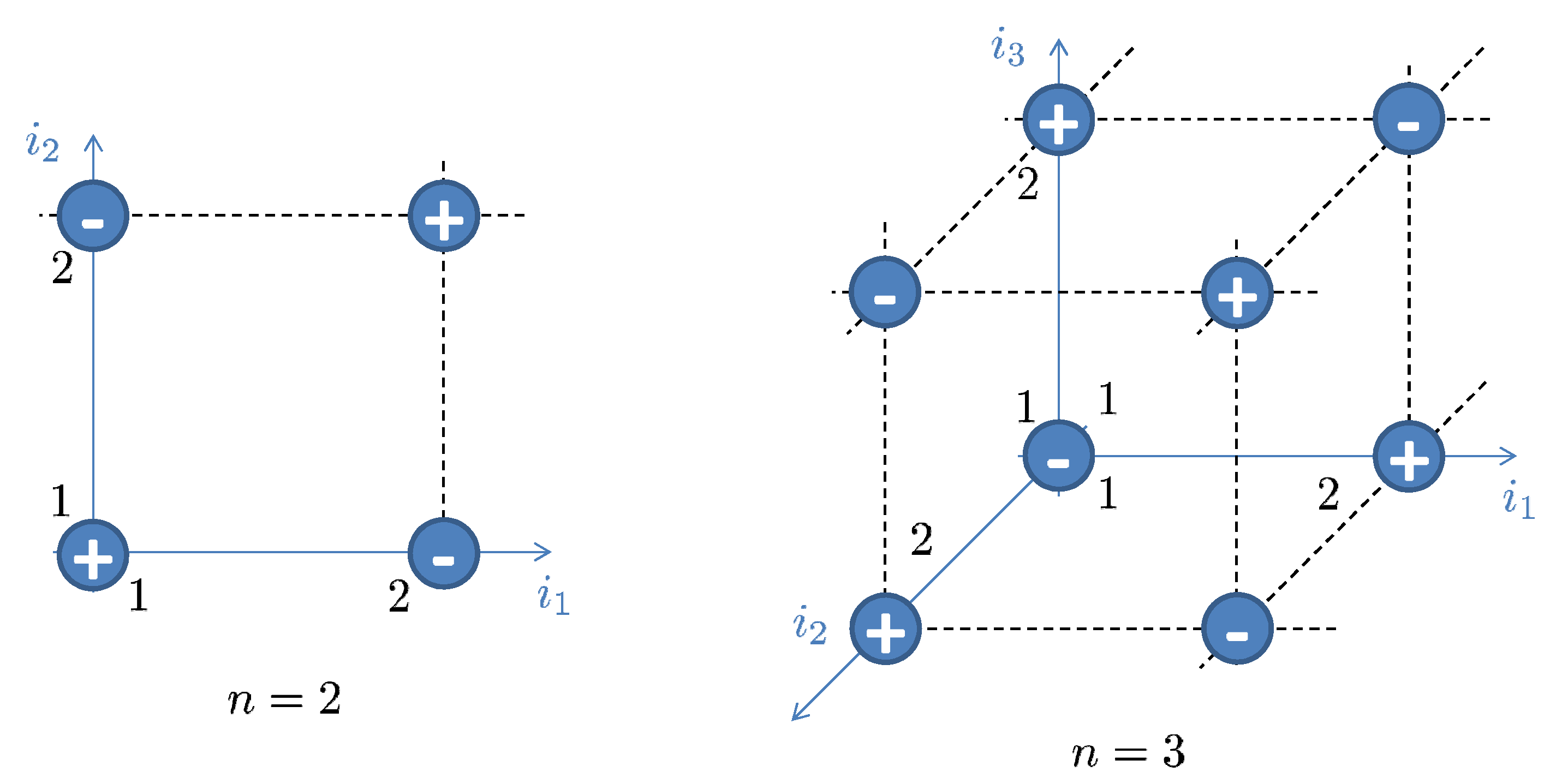
introducing ${\varphi }_{j_1,j_2,\dots }=\mathrm{F}({\zeta }_{1,j_1},{\zeta }_{2,j_2},\dots )$. The summation sign pattern for values of F, or equivalently ${\varphi }_{i_1,i_2,\dots }$, may be best illustrated graphically, as seen in Figure 4.

The following elementary, yet critical, observation can be made and is given as Proposition 3.

Proposition 3.

Along with pmf $\mathbf{p}\in {\Re }^{m^n}$, consider the c.d.f. $\mathbf{ß}\in {\Re }^{m^n}$ and the survival function $\mathbf{s}\in {\Re }^{m^n}$, defined by the corresponding linear transformations

$$\begin{array}{c}\hfill {\displaystyle \Pi : \mathbf{p}\mapsto \mathbf{ß},defined as {\mathbf{ß}}_{\mathbf{i}}=\sum _{\mathbf{j}\le \mathbf{i}}{\mathbf{p}}_{\mathbf{j}} \mathit{and} S: \mathbf{p}\mapsto \mathbf{s}, defined as {\mathbf{s}}_{\mathbf{i}}=\sum _{\mathbf{j}\ge \mathbf{i}}{\mathbf{p}}_{\mathbf{j}}.}\end{array}$$

Then, for any $\mathbf{z}\in {\Re }^{m^n}$ we have

$$\begin{array}{c}\hfill {\displaystyle {\mathbf{p}}^T\mathbf{z}=\sum _{\mathcal{I}}{\mathbf{p}}_{\mathbf{i}} {\mathbf{z}}_{\mathbf{i}}={\left({\Pi }^{-1}\mathbf{z}\right)}^T\left(\mathrm{S}\mathbf{p}\right)={\left({\mathrm{S}}^{-1}\mathbf{z}\right)}^T\left(\Pi \mathbf{p}\right).}\end{array}$$

The proof of the above proposition, although somewhat tedious, simply relies on accounting for the indices in the summation ${\displaystyle \sum _{\mathcal{I}}{\mathbf{p}}_{\mathbf{i}} {\mathbf{z}}_{\mathbf{i}}}$. We also note that for $n=2$, the c.d.f. ordering of two distributions with identical marginals is equivalent to the ordering of the survival functions.

Lemma 1.

Let the two bivariate discrete random variables ${\mathbf{X}}^{\left(1\right)}$ and ${\mathbf{X}}^{\left(2\right)}$ have identical marginals and the corresponding c.d.f. ${\mathbf{ß}}^{\left(1\right)},{\mathbf{ß}}^{\left(2\right)}$. Then, ${\mathbf{ß}}_{\mathbf{i}}^{\left(1\right)}\le {\mathbf{ß}}_{\mathbf{i}}^{\left(2\right)}, \forall \mathbf{i}$, if and only if ${\mathbf{s}}_{\mathbf{i}}^{\left(1\right)}\le {\mathbf{s}}_{\mathbf{i}}^{\left(2\right)}, \forall \mathbf{i}$.

The proof is a straightforward implication of the inclusion–exclusion type fact that

$$\begin{array}{c}\hfill Pr\left(X_1>x_1,X_2>x_2\right)=1-Pr\left(X_1\le x_1\right)-Pr\left(X_2\le x_2\right)+Pr\left(X_1\le x_1,X_2\le x_2\right).\end{array}$$

Finally, we are now able to prove Theorem 4.

Proof of Theorem 4.

The sub-problem (6) can be re-parameterized using the survival function ${\mathbf{s}}_{\mathbf{i}}$,

$$\begin{array}{c}\hfill \begin{array}{cc}\underset{\_}{\mathrm{v}}\left(t\right)=\hfill & {\displaystyle \underset{\mathbf{s}}{inf}{\left({\Pi }^{-1}{(\mathbf{z}-t)}_{+}\right)}^T \mathbf{s}\left({\displaystyle \equiv \underset{\mathbf{p}}{inf}{(\mathbf{z}-t)}_{+}^T {\mathrm{S}}^{-1}\mathrm{S}\mathbf{p} }\right)}\hfill \\ \mathrm{s}.\mathrm{t}.\hfill & {\displaystyle {\underset{\_}{\mathbf{S}}}_{\mathbf{i}}\le {\mathbf{s}}_{\mathbf{i}}\le {\overline{\mathbf{S}}}_{\mathbf{i}}, \mathrm{for} \mathrm{all} \mathbf{i}\in \mathcal{I},}\hfill \\ & {\displaystyle {\mathbf{s}}_{\mathbf{i}}=\frac{m-k+1}{m}, \mathrm{for} \mathrm{all} \mathbf{i}=(1,k) \mathrm{or} (k,1), k=1,\dots ,m,}\hfill \\ & {\displaystyle {\mathbf{s}}_{(1,1)}=1,}\hfill \\ & {\displaystyle {\mathrm{S}}^{-1}\mathbf{s}\ge 0,}\hfill \end{array}\end{array}$$

(11)

where the survival function bounds ${\underset{\_}{\mathbf{S}}}_{\mathbf{i}},{\overline{\mathbf{S}}}_{\mathbf{i}}$ may easily be computed applying the inclusion–exclusion type formula similar to that in Lemma 1.

We now make a critical observation, that ${\Pi }^{-1}{(\mathbf{z}-t)}_{+}\ge 0$ for all t. From the definition of aggregate risk values $\mathbf{z}$, we observe that ${\Pi }^{-1}{(\mathbf{z}-t)}_{+}\ge 0$ if and only if the rectangle inequality (9) holds for all

$$\begin{array}{c}\hfill \begin{array}{cc}{\varphi }_{1,1}={\left(x_{1,i_1}+x_{2,i_2}-t\right)}_{+}\equiv {\left({\mathbf{z}}_{(i_1,i_2)}-t\right)}_{+},\hfill & {\varphi }_{1,2}={\left(x_{1,i_1}+x_{2,i_2^{\prime }}-t\right)}_{+}\equiv {\left({\mathbf{z}}_{(i_1,i_2^{\prime })}-t\right)}_{+},\hfill \\ {\varphi }_{2,1}={\left(x_{1,i_1^{\prime }}+x_{2,i_2}-t\right)}_{+}\equiv {\left({\mathbf{z}}_{(i_1^{\prime },i_2)}-t\right)}_{+},\hfill & {\varphi }_{2,2}={\left(x_{1,i_1^{\prime }}+x_{2,i_2^{\prime }}-t\right)}_{+}\equiv {\left({\mathbf{z}}_{(i_1^{\prime },i_2^{\prime })}-t\right)}_{+},\hfill \end{array}\end{array}$$

with $1\le i_1<i_1^{\prime }\le m, 1\le i_2<i_2^{\prime }\le m$ and any t. Since $x_{1,i_1}\le x_{1,i_1^{\prime }}$ and $x_{2,i_2}\le x_{2,i_2^{\prime }}$, we also have partial ordering of $\zeta$ values, namely

$$\begin{array}{c}\hfill {\varphi }_{1,1}\le {\varphi }_{1,2}\le {\varphi }_{2,2} \mathrm{and} {\varphi }_{1,1}\le {\varphi }_{2,1}\le {\varphi }_{2,2}.\end{array}$$

The range of all t values may clearly be partitioned into ${\mathcal{T}}_{-}=(-\infty ,{\mathbf{z}}_{(i_1,i_2)}]$, $\mathcal{T}=({\mathbf{z}}_{(i_1,i_2)},{\mathbf{z}}_{(i_1^{\prime },i_2^{\prime })})$ and ${\mathcal{T}}_{+}=[{\mathbf{z}}_{(i_1^{\prime },i_2^{\prime })},\infty )$. Therefore, there are three possible cases.

(a)

$t\in {\mathcal{T}}_{-}$: rectangle inequality (9) clearly holds as

$$\begin{array}{c}\hfill 0=\left(x_{1,i_1}+x_{2,i_2}-t\right)-\left(x_{1,i_1}+x_{2,i_2^{\prime }}-t\right)-\left(x_{1,i_1^{\prime }}+x_{2,i_2}-t\right)+\left(x_{1,i_1^{\prime }}+x_{2,i_2^{\prime }}-t\right).\end{array}$$

(b)

$t\in \mathcal{T}$: the validity of the rectangle inequality may easily be established by assuming, without a loss in generality, that ${\mathbf{z}}_{(i_1,i_2^{\prime })}\le {\mathbf{z}}_{(i_1^{\prime },i_2)}$ and considering further sub-cases depending on where the value of t falls with respect to $\mathbf{z}$ subintervals. For example, if $t\in ({\mathbf{z}}_{(i_1,i_2)},{\mathbf{z}}_{(i_1,i_2^{\prime })}]$, then ${\varphi }_{1,1}>{\mathbf{z}}_{(i_1,i_2)}-t$, and thus, the rectangle inequality results in positive mass. That is,

$$\begin{array}{c}\hfill 0<{\left(x_{1,i_1}+x_{2,i_2}-t\right)}_{+}-\left(x_{1,i_1}+x_{2,i_2^{\prime }}-t\right)-\left(x_{1,i_1^{\prime }}+x_{2,i_2}-t\right)+\left(x_{1,i_1^{\prime }}+x_{2,i_2^{\prime }}-t\right).\end{array}$$

(c)

$t\in {\mathcal{T}}_{+}$: clearly the inequality holds as all $\varphi$ values are 0.

Therefore, ${\Pi }^{-1}{(\mathbf{z}-t)}_{+}\ge 0$ indeed holds.

To complete the proof, consider problem (11), where $\underset{\_}{\mathbf{S}}$ and $\overline{\mathbf{S}}$ correspond to ${\mathbf{X}}^{\left(1\right)}$ and ${\mathbf{X}}^{\left(2\right)}$, respectively. Due to the non-negativity of the objective coefficients ${\Pi }^{-1}{(\mathbf{z}-t)}_{+}$ in (11), clearly ${\underset{\_}{\mathrm{CVaR}}}_{\alpha }$ corresponds to ${\mathbf{X}}^{\left(1\right)}$. Similarly, considering a variant of (11) to evaluate the upper ${\overline{\mathrm{CVaR}}}_{\alpha }$ bound, we conclude that ${\overline{\mathrm{CVaR}}}_{\alpha }$ corresponds to ${\mathbf{X}}^{\left(2\right)}$. The fact that ${\underset{\_}{\mathrm{CVaR}}}_{\alpha }\le {\overline{\mathrm{CVaR}}}_{\alpha }$ completes the proof.  □

6.2. A Few Possible Generalizations and Some Counter-Examples

We first provide the definitions of some stochastic ordering and for two multivariate risks ${\mathbf{X}}^{\left(1\right)},{\mathbf{X}}^{\left(2\right)}\in {\Re }^n$ we define

• upper-orthant ordering ${\mathbf{X}}^{\left(1\right)}{⪯}_{uo}{\mathbf{X}}^{\left(2\right)}$ if $Pr({\mathbf{X}}^{\left(1\right)}>\mathbf{x})\le Pr({\mathbf{X}}^{\left(2\right)}>\mathbf{x})$ for all $\mathbf{x}\in {\Re }^n$;
• lower-orthant ordering ${\mathbf{X}}^{\left(1\right)}{⪯}_{lo}{\mathbf{X}}^{\left(2\right)}$ if $Pr({\mathbf{X}}^{\left(1\right)}\le \mathbf{x})\le Pr({\mathbf{X}}^{\left(2\right)}\le \mathbf{x})$ for all $\mathbf{x}\in {\Re }^n$;
• concordance ordering ${\mathbf{X}}^{\left(1\right)}{⪯}_{co}{\mathbf{X}}^{\left(2\right)}$ if ${\mathbf{X}}^{\left(1\right)}{⪯}_{uo}{\mathbf{X}}^{\left(2\right)}$ and ${\mathbf{X}}^{\left(1\right)}{⪯}_{lo}{\mathbf{X}}^{\left(2\right)}$;
• persistent ordering ${\mathbf{X}}^{\left(1\right)}{⪯}_{po}{\mathbf{X}}^{\left(2\right)}$ if ${\mathbf{X}}^{\left(1\right)}{⪯}_{uo}{\mathbf{X}}^{\left(2\right)}$ and ${\mathbf{X}}^{\left(1\right)}{⪰}_{lo}{\mathbf{X}}^{\left(2\right)}$.

Note that, due to Lemma 1, persistent ordering for $n=2$ results in identical distributions, and is therefore not interesting to be investigated for the bivariate case. Recall from the proof of Theorem 4, that for $n=2$, the persistence of CVaR ordering relies on the implied upper-orthant stochastic ordering of the respective risks. Consequently, in search of an extension of such a result to $n=3$, the following question appears to be a natural place to start: Is it true that for trivariate distributions ${\mathbf{X}}^{\left(1\right)}{⪯}_{uo}{\mathbf{X}}^{\left(2\right)}$, we have ${\mathrm{CVaR}}_{\alpha }\left(Z^{\left(1\right)}\right)\le {\mathrm{CVaR}}_{\alpha }\left(Z^{\left(2\right)}\right)$ for all $\alpha \in (0,1)$, with $Z^{\left(1\right)},Z^{\left(2\right)}$ being the corresponding aggregate risks?

From now on, we fix $n=3$ and the marginals of ${\mathbf{X}}^{\left(1\right)},{\mathbf{X}}^{\left(2\right)}$ to be uniform. The key to constructing a counter-example to the above is the failure of the rectangle inequality (10) over ${(\mathbf{z}-t)}_{+}$ values. In turn, this results in a re-parameterized three-dimensional analogue of (11) that has both positive and negative objective coefficients ${\Pi }^{-1}{(\mathbf{z}-t)}_{+}$ for some suitably chosen t. Specifically, consider the only relevant CVaR estimation values of t that correspond to ${\mathbf{z}}_{\mathbf{i}}, \mathbf{i}\in \mathcal{I}$, in accordance with Theorem 2. We claim that for carefully chosen $\mathbf{z}$, we can pick two values $t_{+}$ and $t_{\pm }$ such that ${\Pi }^{-1}{(\mathbf{z}-t_{+})}_{+}\ge 0$, while ${\Pi }^{-1}{(\mathbf{z}-t_{\pm })}_{+}$ contains both positive and negative entries. As a consequence of ${\Pi }^{-1}{(\mathbf{z}-t_{+})}_{+}$ being sign-indeterminant, when estimating ${\underset{\_}{\mathrm{CVaR}}}_{\alpha },{\overline{\mathrm{CVaR}}}_{\alpha }$ with bounds $\underset{\_}{\mathbf{S}},\overline{\mathbf{S}}$ corresponding to the respective distributions ${\mathbf{X}}^{\left(1\right)},{\mathbf{X}}^{\left(2\right)}$, it is natural to expect that we may end up having ${\underset{\_}{\mathrm{CVaR}}}_{\alpha }<{\overline{\mathrm{CVaR}}}_{\alpha }$ for some values of $\alpha$ as well as ${\underset{\_}{\mathrm{CVaR}}}_{\alpha }>{\overline{\mathrm{CVaR}}}_{\alpha }$ for other values of $\alpha$. From here, it may simply suffice to pick “correct” scaling constants $\alpha$ in extremal characterisations of $\mathrm{CVaR}$.

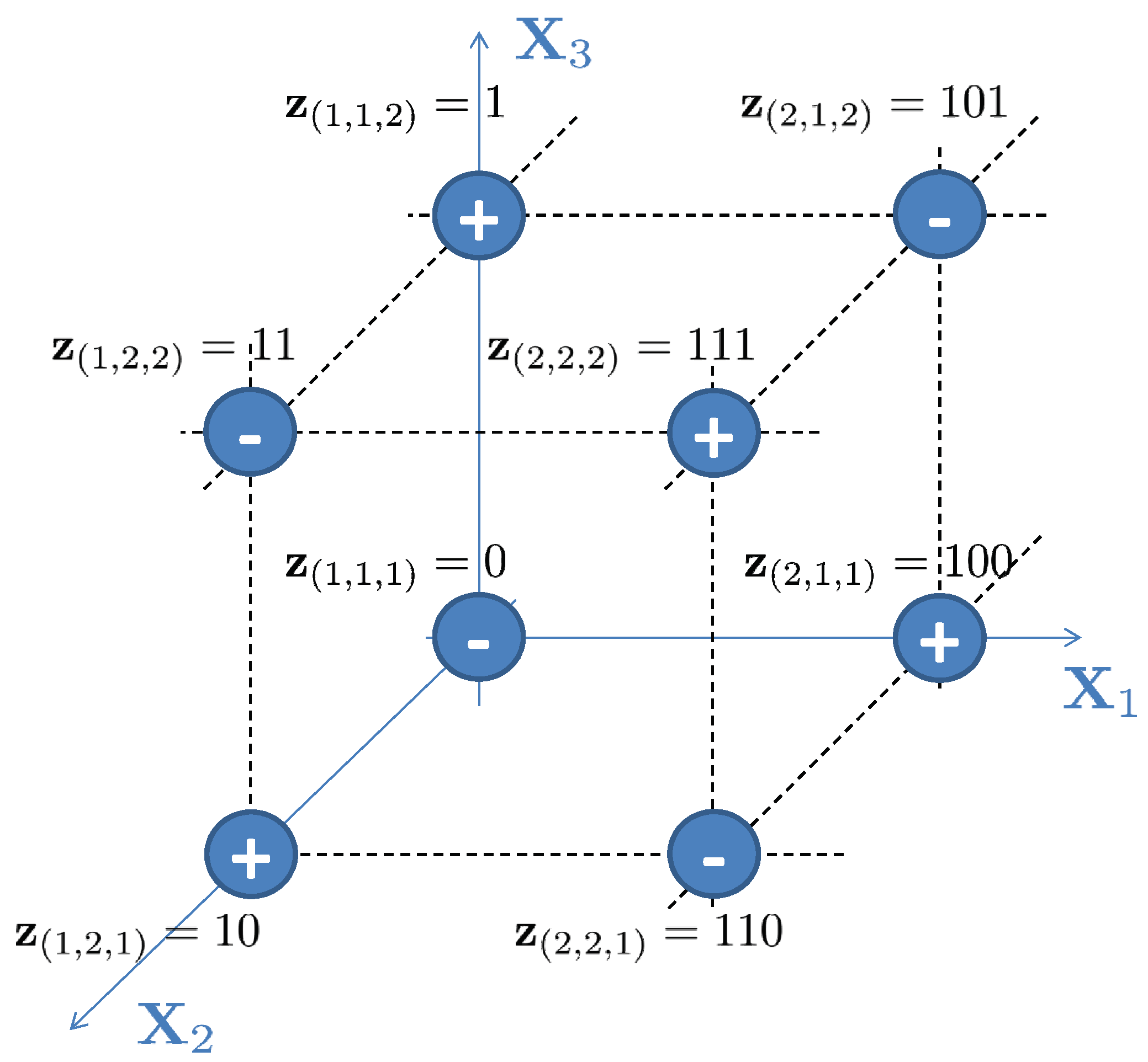
To make this precise, consider the set of risk values for $m=2$ and $m=3$ in

Table 5. Trivariate risk sample values.

Risk	${\mathit{x}}_{\mathit{i},1}$	${\mathit{x}}_{\mathit{i},2}$	${\mathit{x}}_{\mathit{i},3}$
$i=1$	0	100	200
$i=2$	0	10	20
$i=3$	0	1	2

, with aggregate risk values depicted on the hypercube lattice in Figure 5. Take $t_{+}=0$, $t_{\pm }=1$. Clearly, rectangle inequality (10) holds at $t_{+}$ and results in negative mass at $t_{\pm }$, due to the fact that ${({\varphi }_{1,1,1}-t)}_{+}>{\varphi }_{1,1,1}-t$.

Now, we can use $\mathbf{z}$ values to produce a desired counter-example for upper-orthant ordering. To do so, we can form an LP problem to maximize the difference between two partial value-type estimates ${\sum }_{\mathcal{I}}{(\mathbf{z}-t)}_{+} {\mathbf{p}}^{\left(1\right)}$ and ${\sum }_{\mathcal{I}}{(\mathbf{z}-t)}_{+} {\mathbf{p}}^{\left(2\right)}$. We subject both pmfs ${\mathbf{p}}^{\left(1\right)}$ and ${\mathbf{p}}^{\left(2\right)}$ to have identical marginals, and the resulting survival functions ${\mathbf{s}}^{\left(1\right)}=\mathrm{S}{\mathbf{p}}^{\left(1\right)}$ and ${\mathbf{s}}^{\left(2\right)}=\mathrm{S}{\mathbf{p}}^{\left(2\right)}$ to satisfy the upper-orthant ordering, i.e., ${\mathbf{s}}^{\left(1\right)}\le {\mathbf{s}}^{\left(2\right)}$. The last problem can be solved for all $t={\mathbf{z}}_{\mathbf{i}}, \mathbf{i}\in \mathcal{I}$, to extract an example.

A similar exercise can be carried out for the other stochastic orderings. Thus, for the sake of brevity, we give only a summary of our findings in

Table 6. Cases in which ${\mathrm{CVaR}}_{\alpha }\left(Z^{\left(1\right)}\right)>{\mathrm{CVaR}}_{\alpha }\left(Z^{\left(2\right)}\right)$.

Ordering	$\mathit{\alpha }$	i	$p_{(1,1,1)}^{\left(\mathit{i}\right)}$	$p_{(2,1,1)}^{\left(\mathit{i}\right)}$	$p_{(1,2,1)}^{\left(\mathit{i}\right)}$	$p_{(2,2,1)}^{\left(\mathit{i}\right)}$	$p_{(1,1,2)}^{\left(\mathit{i}\right)}$	$p_{(2,1,2)}^{\left(\mathit{i}\right)}$	$p_{(1,2,2)}^{\left(\mathit{i}\right)}$	$p_{(2,2,2)}^{\left(\mathit{i}\right)}$
${⪯}_{uo}$	0.1	1	1/4	-	-	1/4	-	1/4	1/4	-
		2	-	1/4	1/4	-	1/4	-	-	1/4
${⪯}_{lo}$	0.9	1	-	1/4	1/4	-	1/4	-	-	1/4
		2	1/4	-	-	1/4	-	1/4	1/4	-
${⪯}_{po}$	0.1	1	1/4	-	-	1/4	-	1/4	1/4	-
		2	-	1/4	1/4	-	1/4	-	-	1/4

and

Table 7. Cases in which ${\mathrm{CVaR}}_{\alpha }\left(Z^{\left(1\right)}\right)<{\mathrm{CVaR}}_{\alpha }\left(Z^{\left(2\right)}\right)$.

Ordering	$\mathit{\alpha }$	i	$p_{(1,1,1)}^{\left(\mathit{i}\right)}$	$p_{(2,1,1)}^{\left(\mathit{i}\right)}$	$p_{(1,2,1)}^{\left(\mathit{i}\right)}$	$p_{(2,2,1)}^{\left(\mathit{i}\right)}$	$p_{(1,1,2)}^{\left(\mathit{i}\right)}$	$p_{(2,1,2)}^{\left(\mathit{i}\right)}$	$p_{(1,2,2)}^{\left(\mathit{i}\right)}$	$p_{(2,2,2)}^{\left(\mathit{i}\right)}$
${⪯}_{uo}$	0.9	1	1/4	-	-	1/4	-	1/4	1/4	-
		2	-	1/4	1/4	-	1/4	-	-	1/4
${⪯}_{lo}$	0.1	1	-	1/4	1/4	-	1/4	-	-	1/4
		2	1/4	-	-	1/4	-	1/4	1/4	-
${⪯}_{po}$	0.9	1	1/4	-	-	1/4	-	1/4	1/4	-
		2	-	1/4	1/4	-	1/4	-	-	1/4

. In order to verify the results, it suffices to perform a direct calculation. For instance, with respect to the upper-orthant ordering, observe that $Z^{\left(1\right)}$ takes values 0, 11, 101, and 110, and $Z^{\left(2\right)}$ takes values 1, 10, 100, and 111 all with equal probabilities of one-quarter. Consequently, ${\mathrm{CVaR}}_{.1}\left(Z^{\left(1\right)}\right)=61\frac{2}{3}$ and ${\mathrm{CVaR}}_{.1}\left(Z^{\left(2\right)}\right)=61\frac{5}{9}$. Further, one can verify that ${\mathrm{CVaR}}_{\alpha }\left(Z^{\left(1\right)}\right)>(<){\mathrm{CVaR}}_{\alpha }\left(Z^{\left(2\right)}\right)$ holds for any $\alpha <(>).5$.

Interestingly, counter-examples to lower/upper-orthant and persistent orderings require a distribution supported at vertices of a single hypercube, that is, $m=2$. On the other hand, the concordant ordering appears to require more degrees of freedom, e.g., $m=3$. Note that in the latter case, due to the risks being potentially supported on $m^n=27$ vertices, we present the example in a “sparse” format, as seen in

Table 8. Trivariate concordant risks with ${\mathrm{CVaR}}_{.5}\left(Z^{\left(1\right)}\right)>{\mathrm{CVaR}}_{.5}\left(Z^{\left(2\right)}\right)$ and ${\mathrm{CVaR}}_{.9}\left(Z^{\left(1\right)}\right)<{\mathrm{CVaR}}_{.9}\left(Z^{\left(2\right)}\right)$.

i	(2,1,1)	(3,1,1)	(2,3,1)	(3,3,1)	(1,2,2)	(2,1,3)	(3,1,3)	(2,3,3)	(3,3,3)
${\mathbf{z}}_{\mathbf{i}}$	100	200	120	220	11	102	202	122	222
${\mathbf{p}}_{\mathbf{i}}^{\left(1\right)}$	1/6	-	-	1/6	1/3	-	1/6	1/6	-
${\mathbf{p}}_{\mathbf{i}}^{\left(2\right)}$	-	1/6	1/6	-	1/3	1/6	-	-	1/6

.

7. Conclusions

The problem of finding the entire spectrum of values for CVaR of a sum of dependent random variables under dependence uncertainty could be approached in various ways. Under restrictive assumptions, analytical approaches are implementable, but the bounds are often loose, and occasionally, not sharp. Even if the sharpness issue is not present, the lower and upper bounds are typically attained under dependence models that are difficult to justify as feasible in practice, especially for portfolios consisting of many risks, since such extreme dependence models are not realistic.

Our contribution is two-fold. Firstly, we provide a first-in-its-class numerical method for constrained CVaR estimation, when the marginal distributions are known while only the bounds are available for the joint distribution. The latter setting is backed up by many observational data, where the dependence structure is rarely computable even if multivariate observational data are available. As a result, the lower and upper sharp bounds of the CVaR-based aggregate risk can be found. We analyse the complexity of the proposed methods for calculating these bounds, as well as substantiate our findings via numerical illustrations. Our approach trivially generalizes to non-uniform marginals. Despite the fact that the computational cost increases very rapidly with the number of risks, we believe that the method may still be used as a viable exploratory tool when dealing with a relatively large risk portfolio. Finally, we show how the run-times may be significantly improved, by exploiting the very special structure of the underlying linear optimization problems at the formulation stage.

Secondly, it is known that CVaR respects the so-called lower-orthant stochastic ordering for two-dimensional portfolios. Yet, no similar result has yet been established or disproved for higher dimensions. As a by-product of our analysis, using elementary LP techniques, we show that no such extensions are possible. Specifically, we construct trivariate counter-examples that demonstrate a lack of aggregate risk monotonicity under upper, lower-orthant, concordant, and persistent stochastic orderings. We also give a self-contained alternative proof for the bivariate risk case, and point out the exact reason why higher-dimensional extensions are not possible.

References

- Acerbi, Carlo, and Dirk Tasche. 2002. On the Coherence of Expected Shortfall. Journal of Banking and Finance 26: 1487–503. [Google Scholar] [CrossRef]
- Asimit, Alexandru V., Alexandru M. Badescu, Steven Haberman, and Eun-Seok Kim. 2016. Efficient risk allocation within a non-life insurance group under Solvency II Regime. Insurance: Mathematics and Economics 66: 69–76. [Google Scholar] [CrossRef]
- Asimit, Alexandru V., Junlei Hu, and Yuantao Xie. 2019. Optimal Robust Insurance with a Finite Uncertainty Set. Insurance: Mathematics and Economics 87: 67–81. [Google Scholar] [CrossRef]
- Asimit, Alexandru V., Valeria Bignozzi, Ka Chun Cheung, Junlei Hu, and Eun-Seok Kim. 2017. Robust and Pareto Optimality of Insurance Contract. European Journal of Operational Research 262: 720–32. [Google Scholar] [CrossRef]
- Balbás, Alejandro, Beatriz Balbás, and Antonio Heras. 2011. Stable Solutions for Optimal Reinsurance Problems involving Risk Measures. European Journal of Operational Research 214: 796–804. [Google Scholar] [CrossRef]
- BCBS. 2016. Standards. In Minimum Capital Requirements for Market Risk. Basel Committee on Banking Supervision. Basel: Bank for International Settlements, January. [Google Scholar]
- Ben-Tal, Aharon, Laurent El Ghaoui, and Arkadi Nemirovski. 2009. Robust Optimization. Princeton: Princeton University Press. [Google Scholar]
- Bertsimas, Dimitris, and Ioana Popescu. 2002. On the Relation between Option and Stock Prices: A Convex Optimization Approach. Operations Research 50: 358–74. [Google Scholar] [CrossRef]
- Bertsimas, Dimitris, Geoffrey J. Lauprete, and Alexander Samarov. 2004. Shortfall as a Risk Measure: Properties, Optimization and Applications. Journal of Economic Dynamics and Control 28: 1353–81. [Google Scholar] [CrossRef]
- Billingsley, Patrick. 1995. Probability and Measure, 3rd ed. New York: John Wiley and Sons. [Google Scholar]
- Blanchet, Jose, Henry Lam, Qihe Tang, and Zhongyi Yuan. 2017. Applied Robust Performance Analysis for Actuarial Applications. Technical Report, Society of Actuaries. Available online: https://web.stanford.edu/~jblanche/papers/Robust_Actuarial.pdf (accessed on 5 May 2023).
- Chen, Wenqing, Melvyn Sim, Jie Sun, and Chung-Piaw Teo. 2009. From CVaR to Uncertainty Set: Implications in Joint Chance-Constrained Optimization. Operations Research 58: 470–85. [Google Scholar] [CrossRef]
- Denuit, Michel, Jan Dhaene, Marc Goovaerts, and Rob Kaas. 2005. Actuarial Theory for Dependent Risks: Measures, Orders and Models. Chichester: Wiley. [Google Scholar]
- El Ghaoui, Laurent, Maksim Oks, and Francois Oustry. 2003. Worst-case Value-at-risk and Robust Portfolio Optimization: A conic Programming Approach. Operations Research 51: 543–56. [Google Scholar] [CrossRef]
- Fabozzi, Frank J., Dashan Huang, and Guofu Zhou. 2010. Robust Portfolios: Contributions from Operations Research and Finance. Annals of Operations Research 176: 191–220. [Google Scholar] [CrossRef]
- Gijbels, Irène, and Dominik Sznajder. 2013. Positive Quadrant Dependence Testing and Constrained Copula Estimation. Canadian Journal of Statistics 41: 36–64. [Google Scholar] [CrossRef]
- Gómez, Fabio, Qihe Tang, and Zhiwei Tong. 2022. The Gradient Allocation Principle based on the Higher Moment Risk Measure. Journal of Banking & Finance 143: 106544. [Google Scholar]
- Gurobi Optimization, LLC. 2023. Gurobi Optimizer Reference Manual. Available online: https://www.gurobi.com (accessed on 5 May 2023).
- Huang, Dashan, Shushang Zhu, Frank J. Fabozzi, and Masao Fukushima. 2010. Portfolio Selection under Distributional Uncertainty: A Relative Robust CVaR Approach. European Journal of Operational Research 203: 185–94. [Google Scholar] [CrossRef]
- Rockafellar, R. Tyrrell, and Stanislav Uryasev. 2000. Optimization of Conditional Value-at-Risk. Journal of Risk 2: 21–41. [Google Scholar] [CrossRef]
- Swiss Solvency Test. 2006. FINMA SST Technisches Dokument. Available online: https://www.finma.ch/FinmaArchiv/bpv/download/e/SST_techDok_061002_E_wo_Li_20070118.pdf (accessed on 5 May 2023).
- Tardos, Éva. 1986. A Strongly Polynomial Algorithm to Solve Combinatorial Linear Programs. Operations Research 34: 250–56. [Google Scholar] [CrossRef]
- Zhu, Shushang, and Masao Fukushima. 2009. Worst-Case Conditional Value-at-Risk with Application to Robust Portfolio Management. Operations Research 57: 1155–68. [Google Scholar] [CrossRef]
- Zinchenko, Y. 2023. CVaR Engine for a Sharp Lower Bound, GitHub Repository. Available online: https://github.com/yzinchenko/CVaR (accessed on 5 May 2023).
- Zymler, Steve, Daniel Kuhn, and Berç Rustem. 2013. Worst-case Value-at-risk of Nonlinear Portfolios. Management Science 59: 172–88. [Google Scholar] [CrossRef]
Figure 1.
Perceived behavior of : (a) strict piecewise concavity, (b) convexity.
Figure 2.
Hypothetical concavity of : (a) , (b) .