Intelligent Decision Support in Proportional–Stop-Loss Reinsurance Using Multiple Attribute Decision-Making (MADM)


Department of Industrial Systems Engineering and Management, Faculty of Engineering, National University of Singapore, Singapore 117576, Singapore
*
Author to whom correspondence should be addressed.
J. Risk Financial Manag. 2017, 10(4), 22; https://doi.org/10.3390/jrfm10040022
Submission received: 8 July 2017
/
Revised: 17 November 2017
/
Accepted: 17 November 2017
/
Published: 28 November 2017
(This article belongs to the Special Issue Risk Management Based on Intelligent Information Processing)
Abstract
:This article addresses the possibility of incorporating intelligent decision support systems into reinsurance decision-making. This involves the insurance company and the reinsurance company, and is negotiated through reinsurance intermediaries. The article proposes a decision flow to model the reinsurance design and selection process. This article focuses on adopting more than one optimality criteria under a more generic combinational design of commonly used reinsurance products, i.e., proportional reinsurance and stop-loss reinsurance. In terms of methodology, the significant contribution of the study the incorporation of the well-established decision analysis tool multiple-attribute decision-making (MADM) into the modelling of reinsurance selection. To illustrate the feasibility of incorporating intelligent decision supporting systems in the reinsurance market, the study includes a numerical case study using the simulation software @Risk in modeling insurance claims, as well as programming in MATLAB to realize MADM. A list of managerial implications could be drawn from the case study results. Most importantly, when choosing the most appropriate type of reinsurance, insurance companies should base their decisions on multiple measurements instead of single-criteria decision-making models so that their decisions may be more robust.
1. Introduction
1.1. Background
Reinsurance is generally known as “insurance for insurance”. Following similar concepts and principles as insurance, it provides financial compensation to insurance companies with respect to the risk of large losses. The reinsured party (or “insurance company”) buys reinsurance from the reinsurer (or “reinsurance company”) in exchange for loss limitation, revenue protection, and freeing up of capital. In recent years, reinsurance has grown both in market value and diversity due to worldwide trends such as global climate change, increases in insurance mega losses, volatility in equity markets, and emerging risks such as terrorism. Regardless of financial size, an insurance company rarely retains all of their risk. Thus, it is of interest to understand the decision-making process with respect to the reinsurance contract, which in reality is usually done using negotiation intermediaries, i.e., reinsurance brokers. Typically, there are two categories of reinsurance decisions, both of which will be addressed in this study:
- The optimal reinsurance form, under given criteria;
- Given the reinsurance form, the choice of reinsurance parameters. (e.g., optimal retention portion for proportional reinsurance, optimal retention limit for stop-loss reinsurance, etc.)
This study focuses on treaty reinsurance, which covers an entire portfolio with multiple single risks. Both facultative and treaty reinsurance could be further broken down into proportional reinsurance and non-proportional reinsurance (Carter 1979). Early works have shown that under variance risk measurement with fixed premium, the stop-loss contract is the optimal reinsurance form for reinsurance buyers (Borck 1960; Hürlimann 2011), whereas the quota-share best addresses the interests of the reinsurer (Vajda 1962). Clearly, there would be conflicts of choice between two parties. Thus, this study addresses a combinational form of proportional and stop-loss treaty reinsurance (see Section 3.2), following the definition by Samson and Thomas (1985). Quota-share reinsurance and stop-loss reinsurance could be considered as special cases of proportional–stop-loss reinsurance. In deciding the optimal reinsurance design parameters, this study attempts to utilize multiple-attribute decision-making (MADM) improving on previous works in the literature which use a single criterion.
1.2. Paper Development
The paper is organized as follows. Section 2 reviews the recent research that this study is built upon. Section 3 develops the decision flow based on the form of proportional–stop-loss reinsurance and determines the optimal reinsurance parameters using multi-objective decision-making (MODM). Section 4 includes a numerical case study, which models claims using @Risk and implements MADM for buyer’s selection using MATLAB. Section 5 discusses contributions, limitations, and further directions, and concludes the study.
2. Literature Review
Decision analysis models using limited criterion have been extensively discussed both for the reinsurer in structuring reinsurance and for the reinsured party for evaluating and selecting the most appropriate reinsurance product (Samson and Thomas 1985). Only recently have researchers begun to look into the cooperative behavior of both parties to reach a joint-party optimality. In addition, the recent growth of promising decision analyses based on multiple criteria has ignited sparks in the field of reinsurance research. In particular, this study is developed upon three recent works (Bazaz and Najafabadi 2015; Karageyik and Şahin 2017; Payandeh-Najafabadi and Panahi-Bazaz 2017) which focus on multi-attribute decision-making (MADM) and proportional–stop-loss reinsurance.
Karageyik and Dickson (2016) first proposed using MADM with respect to the problem of selecting optimal reinsurance levels under competing criteria. On choosing the input alternatives, they use ruin probability as a constraint, i.e., the insurance company should not have a probability of ruin greater than 1%. Loss distribution was modeled as the translated gamma process and the forms considered were pure proportional and pure stop-loss reinsurance. The study also includes comparison with single-criterion decision-making and concludes that MADM is extremely insightful for selecting optimal reinsurance.
Later, Karageyik and Şahin (2017) improved on this research by taking value-at-risk (VaR) measurement into consideration, specifically targeting at optimal retention level in excess-of-loss reinsurance design. Key measurement criteria are expected profit, expected shortfall, finite time ruin probability, and variance of risk. By comparing and contrasting different MADM techniques, the authors safely concluded that under the case of reinsurance where correlation between measurements are low enough, different MADM techniques will generate similar optimal retention level.
However, both studies focused either on pure proportional reinsurance or pure non-proportional reinsurance, with neither considering the combination of both. The most contemporary discussion of general reinsurance model took a viewpoint from both the insurer and reinsurer, and based on TVaR measurement, suggesting that a pareto-optimal solution always exists (Cai et al. 2017). The pareto-optimality studies have been successful in addressing multiple decision objectives, especially in trading cases where both seller and buyer parties could simultaneously make decisions on contracts (Trade procedure P1 in Section 3.1). Our approach of using MADM is different from a nest of Multiple Objective Decision Models (MODM) in that MADM is assigning rankings to a cluster of available alternatives. This would be especially useful in settings (Trade procedure P2 in Section 3.2) where buyers may have limited, discrete alternatives to choose from. In such settings, deriving an optimal contract would be less meaningful as such contract may not be in the feasible set faced by the buyer party (the reinsured, in our story).
To the best of my knowledge, there is no previous research conducting ranking of proportional–stop-loss reinsurance alternatives based on multiple measurement schemes while considering decisions from both parties. Thus, this study serves the purpose of filling this gap. Section 3 incorporates two-sided deal procedures into the reinsurance optimality study and describes the procedure of applying MADM to reinsurance selection. Following this, Section 4 includes a case study to model the reinsured party´s choice of reinsurance in real time.
3. Methodology
3.1. Decision Flow
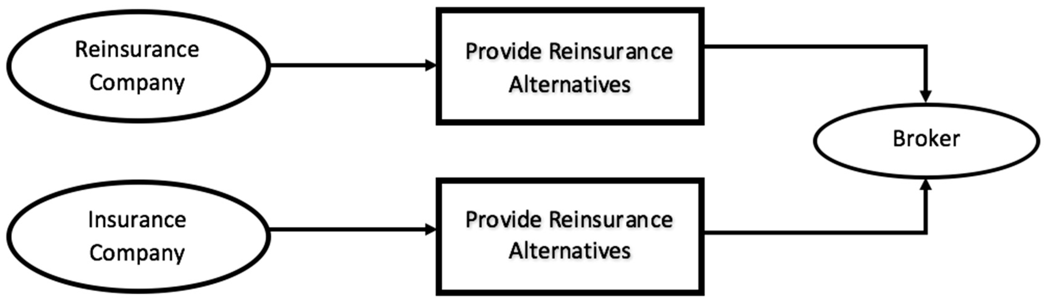
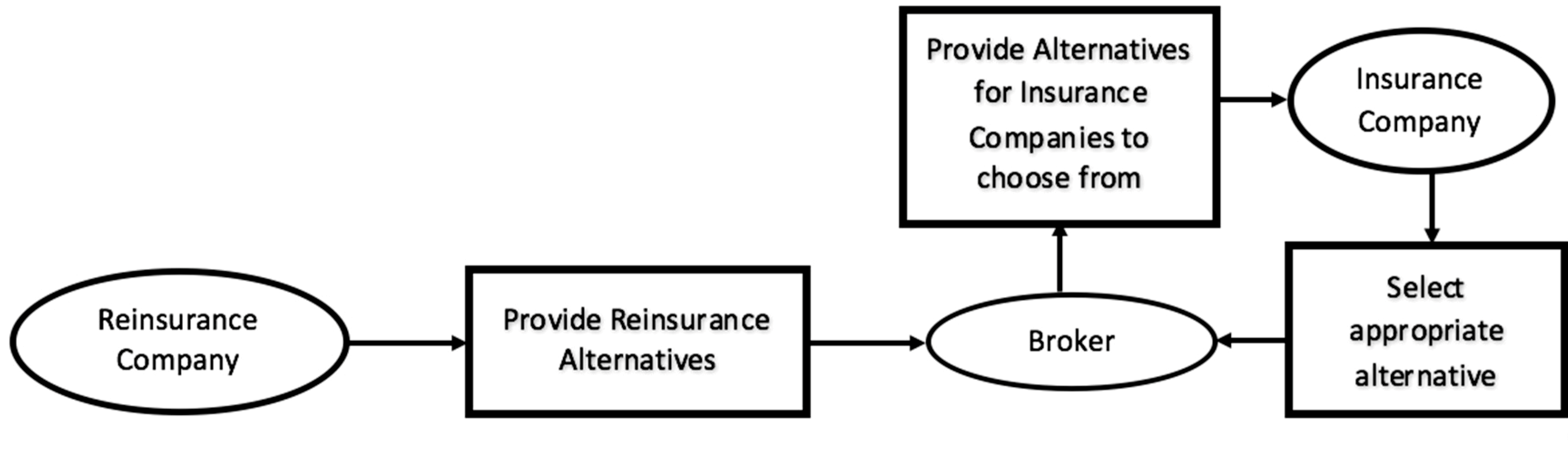
As reinsurance decision-making involves the selling party (the reinsurance company, or the reinsurer) and the buying party (the insurance company, or the reinsured party), it could be safely viewed as a two-sided trade process, which involves negotiation between the selling and buying parties. Furthermore, reinsurance deals could be viewed as the established two-sided trade matching models P1 (Figure 1) or P2 (Figure 2) with the existence of a broker (Liang 2014).
For the first trade procedure P1, both the reinsurer and the reinsured party exchange information through the broker. Previous research on two-sided optimality could largely be viewed as P1 when both firms make decisions simultaneously. In this case, an equilibrium strategy either optimizing one side or both side’s benefits could be reached (see Borch 1960; Wang 2003; Cai et al. 2017), while few works in literature have discussed reinsurance deals settled under procedure P2. Under P2, the seller (the reinsurer) will provide several plans for the buyer to choose from. Noting the prevalence of procedure P2 in reinsurance industry practice, this study attempts to model reinsurance scenarios under P2 by using classic MODM in providing reinsurance alternatives and by using MADM in selecting an appropriate reinsurance design for the reinsured party. The rest of the section follows this decision flow. Section 3.2 defines the proportional-stop-loss reinsurance form; Section 3.4 constructs one simplified set of reinsurer’s offerings using MODM. Section 3.5 defines each of the key criteria the reinsured may consider. Finally, Section 3.6 presents the application of MADM in aiding the decision of ranking the reinsurance alternatives.
3.2. The Proportional–Stop-Loss Reinsurance Model
The paper discusses proportional–stop-loss reinsurance, adopting definitions from Samson and Thomas (1985), Hürlimann (2011) and Payandeh-Najafabadi and Panahi-Bazaz (2017), under which, given a single loss of X and a reinsurance arrangement with parameters , the reinsurer is bonded to pay a claim amount of:
where a is the fraction ceded to the reinsurer and M is the retention limit. The reinsured party will pay the rest of the claim , where represents the amount of claim paid by the reinsurer. When M = 0, the proportional–stop-loss model becomes the classical quota-share reinsurance model, and when a = 1, it becomes the classical stop-loss reinsurance model.
3.3. Variable Definition
To ensure the consistency of notations in this paper, we define the key variables as shown in Table 1. Almost all definitions follow previous literature, and necessary elaborations will be given in later sections.
3.4. Simulating Alternatives Using MODM
Considering the reinsurance practices and following previous research on the joint-party reinsurance problem, we first attempt to model the reinsurer pricing objectives. As such, we provide a list of alternatives for the reinsured party to choose from. We attempt to formulate a model maximizing the reinsurer’s expected profit while minimizing the variance of profit. In deciding a reinsurance design, the reinsurer needs to specify the premium and the arrangement of the reinsurance claim amount, in other words, the reinsurance premium loading factor and the reinsurance design parameter . Under the expected value premium principle, the insurance premium must be at least greater than the expected individual loss (Karageyik and Şahin 2017). Thus, the bi-objective model is formulated as:
where is defined as the aggregated claim of loss (compounded from individual loss ), and is the premium paid to the reinsurance company per unit of time, defined according to the expected value premium principle (formulas are in Section 3.5.1).
Clearly, there is conflict between two objectives and there is no single design of that can achieve all objectives. The closed-form derivations (Hürlimann 2011) are omitted and the optimal solution set would be an efficient frontier analyzed in closed form. The optimal pairs will satisfy:
Note that for an increasing ceding level a, the reinsurer risk and expected profit will both increase proportionally; thus, the reinsurer preference will be ambiguous for different ceding portion while fixing the pair of . This is in line with the work of Payandeh-Najafabadi and Panahi-Bazaz (2017) where it is suggested that optimal design depends on the loss distribution (in our case, ) but not on the market premium () , and does not depend on the portion retained (). Thus, it would be flexible for the reinsurance company to select an appropriate ceding portion given their risk appetite and their financial capability (which is often not necessarily known by the broker). In Section 5, we will briefly discuss the resulting effects of choosing different ceding portions of , based on a numerical case study.
Thus, the alternatives provided by the reinsurance firm will be in the form of . These are inputing alternatives we will use to apply MADM.
3.5. Calculating Decision Criteria
Now, we need to define the selection criteria for reinsurance design. In this study, we are concerned with expected profit, expected shortfall, ruin probability, and expected utility as selection criteria. All of these factors are calculated taking the viewpoints of reinsurance buyers (the reinsured parties).
3.5.1. Expected Profit of the Insurance Company (Reinsured Party):
In general, the expected profit of the reinsured party is calculated as the difference between the insurer’s income and the claims paid to the policyholders. Net premium gained by the insurance company is calculated under the expected value premium principle, defined as:
The net insurance profit after considering the reinsurance arrangement is:
Our objective is to maximize the expected profit of the insurance company.
3.5.2. Expected Shortfall
Expected shortfall is calculated under value at risk (VaR) measurement. VaR, given a confidence level of , is defined as the smallest , such that the probability of loss is at least (Bazaz and Najafabadi 2015), i.e.,
Expected shortfall is the financial risk measurement to investigate market risk of the portfolio. It is calculated as the expected value of tail distribution of as follows:
An increase in retention level M will cause the insurer’s liability to insurance policyholders to increase, and thus ES will increase accordingly. In contrast, a larger ceding portion will release the insurer from burden and thus will decrease the amount of liability held by the reinsured party. Our objective is to find the optimal (a,M) pair that could minimize the expected shortfall of the insurance company.
3.5.3. Ruin Probability
The ruin probability criterion is based on definitions of finite time ruin probability measurement. The insurer’s asset is represented as and is defined by:
In Equation (8) is the net premium income per unit time gained by the insurance company, and S(t) is the aggregate claim amount up to time t, which is calculated by:
The finite time ruin probability, , is given as:
In our study, the ruin probability is approximated through a simulation study, as the closed form ruin probability for compounding exponential loss distribution under proportional–stop-loss reinsurance design is hard to obtain. Our objective is to minimize the ruin probability of such that the insurance company would be less likely to go bankrupt if there is a large loss incurred.
3.5.4. Expected Utility
To address the utility theory used in vast literature on reinsurance optimization (Samson and Thomas 1983), the utility function of the reinsured is defined as exponential utility function, which assumes constant absolute risk aversion:
In reality, utility function may have much more complexity and may be different for different insurance companies. However, as long as the value of utility could be obtained in numeric value, decisions could be made through MADM. In deciding the ranking of reinsurance alternatives, one of our objectives is to maximize the expected utility of the insurance company.
3.6. Selecting the Best Alternative Using MADM
In Section 2, we reviewed decision analysis techniques on reinsurance decisions under single measurement. In order to model the decision of the reinsurance purchasing party (the insurance company or the reinsured) under multiple measurement criteria, this study adopts multi-criteria decision-making techniques. In particular, the Technique for Order of Preference by Similarity to Ideal Solution (TOPSIS), reviewed in prior works (Bazaz and Najafabadi 2015) is the most popular MADM technique and is the most suitable for pure numerical criteria. TOPSIS was originally developed by Hwang and Yoon (1981), and was later developed by Yoon (1987) and Hwang et al. (1993).
TOPSIS is thus applied to the reinsurance selection problem. Furthermore, as suggested by Karageyik and Şahin (2017), the correlation amongst criteria in reinsurance problem is small enough to return similar results from different TOPSIS methodologies. Thus, in this study we choose the classical TOPSIS method to support our analysis.
Following similar definitions of TOPSIS in a previous study (Bazaz and Najafabadi 2015; Ameri Sianaki 2015; Karageyik and Şahin 2017), we briefly describe the steps of applying the method as follows. This study attempts to implement the TOPSIS decision supporting system by storing reinsurance alternatives in Excel and processing the input matrices with a MATLAB code. Part of the MATLAB code was developed with reference to previous efforts by Amari (Ameri Sianaki 2015), and was revised accordingly to serve the needs of this study. Below is the complete procedure of conducting TOPSIS.
- Formulate decision matrix with alternatives and decision criteria . The attribute value of on for and is represented as .
- Calculate weight of the criteria using entropy technique as follows:
- Normalize the decision matrix using the following formula:One may notice that by scaling the criteria (multiplying a constant to ), the decision will not change. However, it will not necessarily return same decision for different utility functions that generate the same decision under expected utility measurement, as adding a constant to in the formula will change the resulting .
- Calculate the weighted normalized decision matrix by using the normalized decision matrix parameter and weight vector ) to return the weighted normalized decision matrix parameter . If criteria are given same weight, .
- Compute the vectors of positive ideal solutions and the negative ideal solutions, denoted by:
- Calculate the distance between each alternative and the positive and negative ideal points. The distance between alternative and the positive ideal points is:The distance between alternative and the negative ideal solutions are:
- Calculate the relative closeness coefficient of each alternative represented as:
- Rank the alternatives according to . The alternative with higher value is preferred over lower alternatives.
A graphical representation of TOPSIS is shown in Figure 3. Each blue ball represents one available alternative. The red ball represents the negative ideal solution and the green ball represents the positive ideal solution. The blue ball that is relatively near to the green ball and away from the red ball would be the best alternative amongst all. Given at least four selection criteria, it would be hard to visualize the alternatives in 3-dimensional space, thus the calculation of distance is coded using MATLAB.
4. Case Study
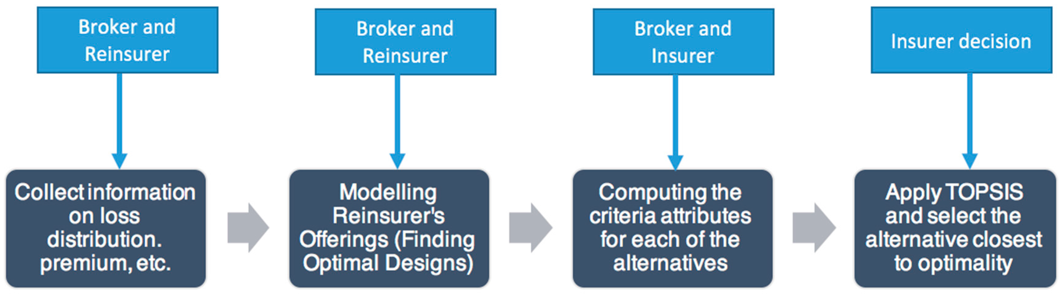
Following the decision flow in Section 3, this study models the reinsurance deal procedure as illustrated in Figure 4. We will choose a loss distribution model in Section 4.1, generate reinsurance offering alternatives in Section 4.2, tabulate the decision matrix in Section 4.3, and finally apply MADM in selecting from alternatives in Section 4.4.
4.1. Loss Distribution Modeling
Under treaty reinsurance, which covers the entire line of insurance business handled by the insurance company, the aggregated claim is a compounding distribution of single risks or claims incurred during time period .
Following the majority of research on modeling losses or claims (e.g., Samson and Thomas 1985; Bazaz and Najafabadi 2015; Payandeh-Najafabadi and Panahi-Bazaz 2017; Karageyik and Şahin 2017); our case study chooses to model individual claims as an exponential loss model with the parameter , i.e.,
The occurrence of a claim follows Poisson distribution with mean , i.e.,
Thus, S is the compounding distribution of identical, independently distributed risks, each with distribution X.
In this case study, we set , and original insurance premium parameter .
4.2. Generating Alternatives from the Viewpoints of Reinsurers
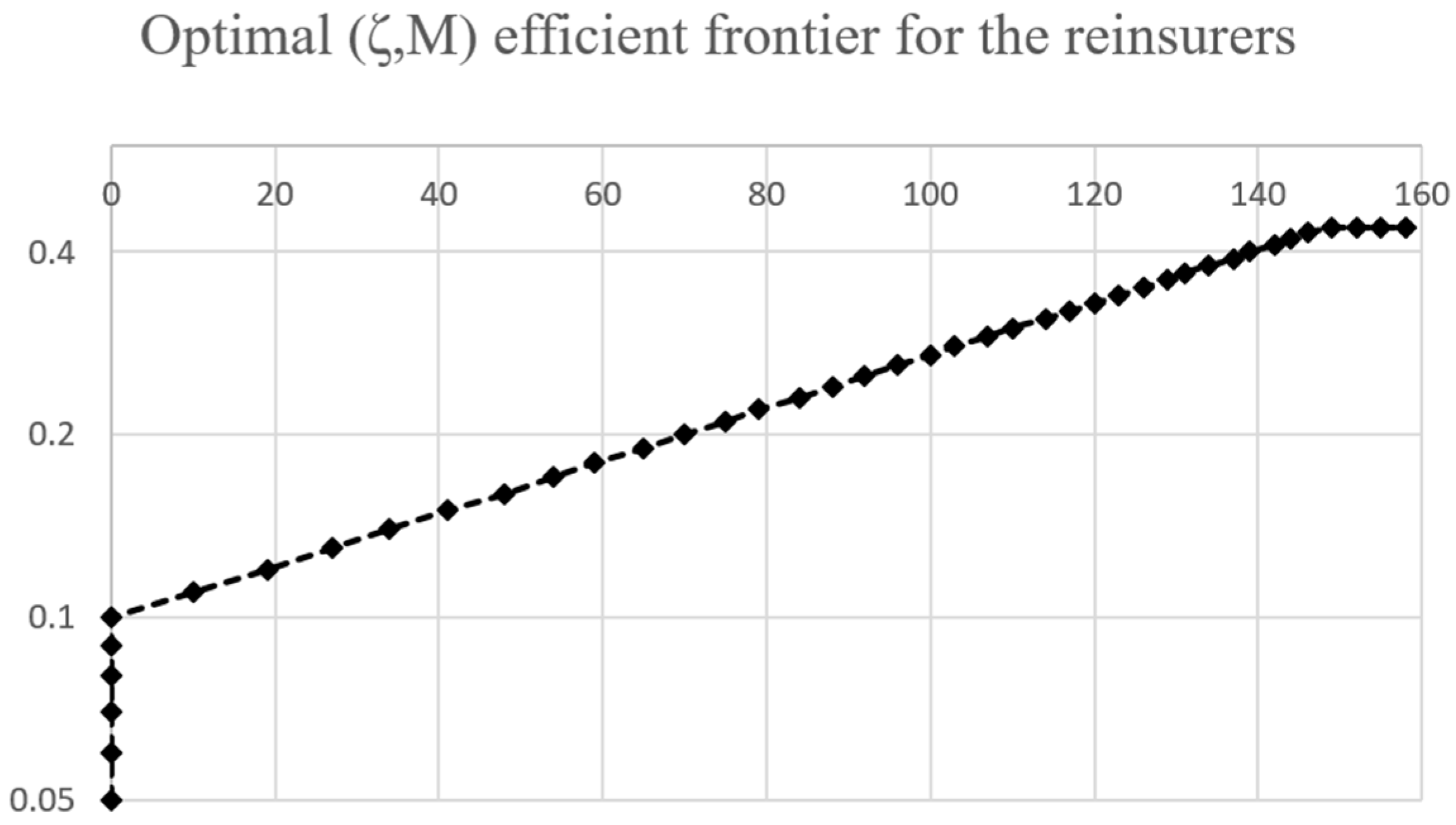
Following Section 3.2, we define the case by setting the portion ceded as a = 0.6, a = 0.75, a = 0.9 and a = 1, respectively, in assessing the differences in results when the retention level is changed. The optimal pair (Figure 5 with on x-axis and M on y-axis) is sought by a grid search, as solving Formula 3.2 in mathematical form may not be succinct.
When , constraint will be violated; all points to the right and below of the efficient frontier are deemed as inferior to the points on the efficient frontier. In managerial terms, the reinsurance designs with parameters to the southeast of the efficient frontier will cause the reinsurance company to likely generate less profit while suffering from a larger risk.
4.3. Constructing Decision Matrix
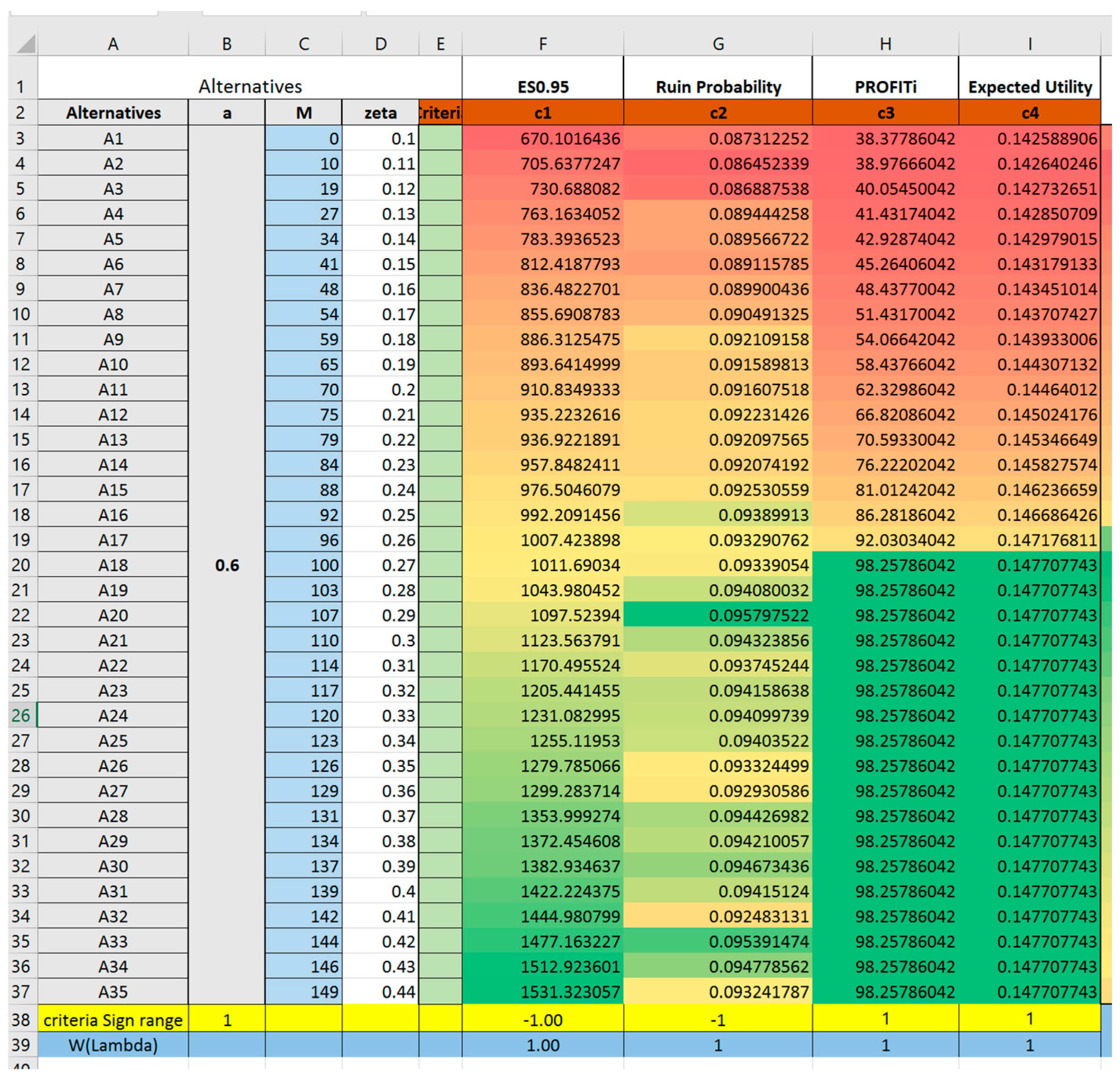
For illustration, Figure 6 shows the optimal pairs of given other parameters in the case study. For the first trial, we fixed the ceding portion at a = 0.6 and select 35 pairs of the optimal as the reinsurance design parameters for TOPSIS alternatives. Profit for the insurance company and expected utility after claims are calculated using theoretical mean of the random distributions. However, given that the claim process compounds exponential loss with Poisson occurrence, ruin probability and expected shortfall at 95% confidence level are hard to obtain in analytic terms. Thus, by using Monte Carlo simulation with 100,000 iterations, losses and claims are modeled as exponential values with Poisson occurrence, and and ruin probability are calculated in Excel as follows in Figure 6:
4.4. Selecting Alternatives Using TOPSIS
With the above alternatives inputting the decision matrix, we observe that if we only consider minimizing expected shortfall and ruin probability, the profit or expected utility will be exceptionally low. The color scale shows intuitively this conflict with red representing smallest value and green representing largest value. We define the weight vector of criteria as all equals (equal values in blue cells Range F39:I39). Recalling the Matlab function built earlier in Section 3 by executing the following code:
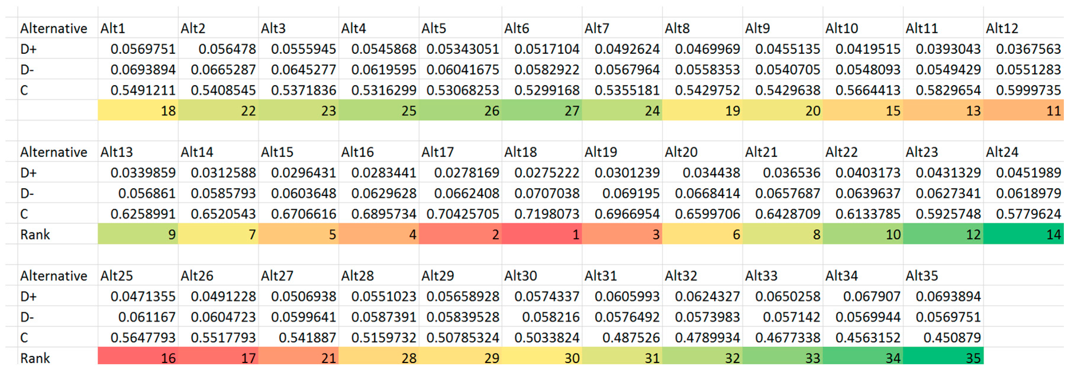
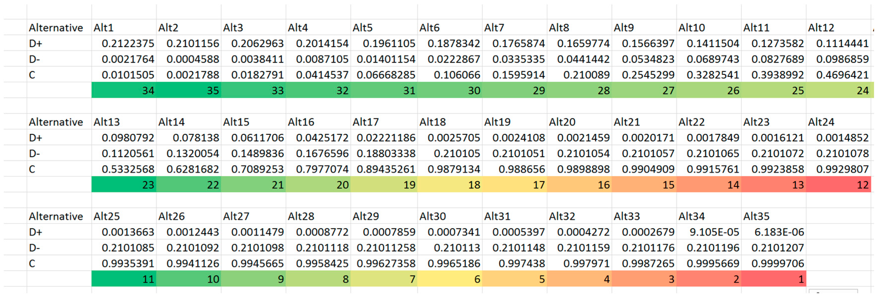
we could get normalized weight matrix, the identified ideal solutions and the distance between each alternative and the ideal optimality. All these results are stored in Excel sheet “TOPSIS OUTPUT Variables” with selection ranking results shown in Figure 8.
| topsis (decisionMakingMatrix,lambdaWeight,criteriaSign) |
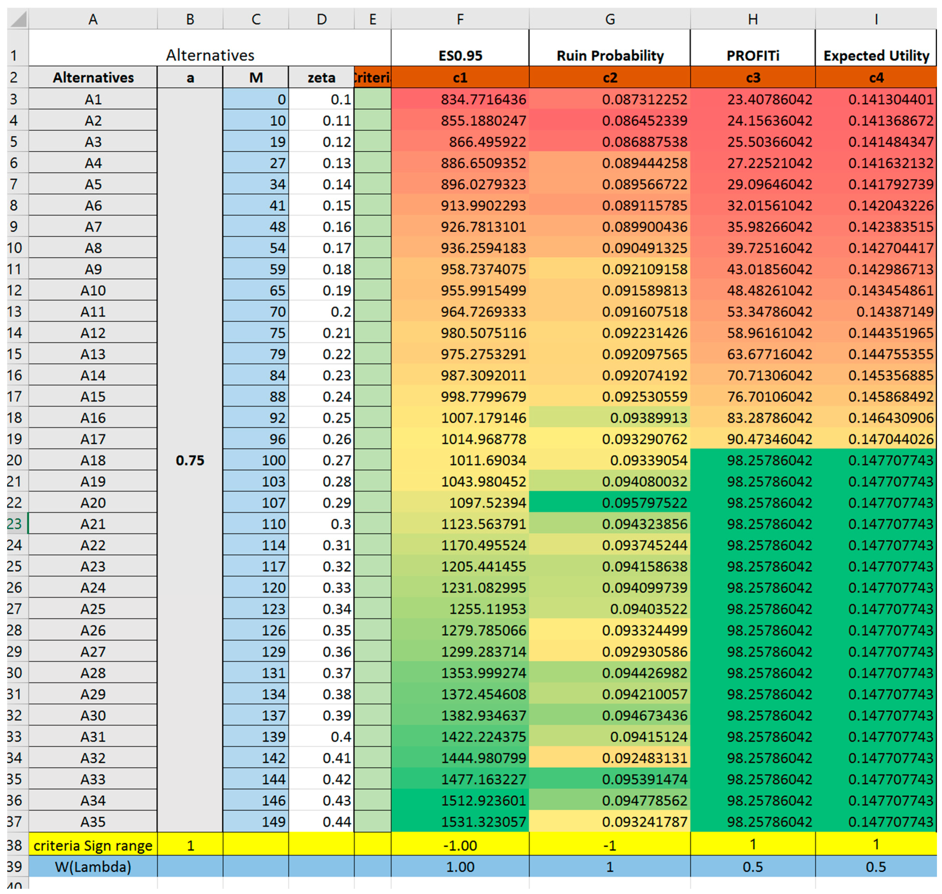
From the TOPSIS output, we could identify that Alternative 18 (0.27, 100) is the best choice, followed closely by Alternative 17 (0.26, 96). Alternative 19 (0.28, 103) is not far away as the third best alternative identified. Alternative 35 (0.44, 149) is the furthest from ideal solution. Multiple trials were tested fixing a at a = 0.75 (Trial 2), a = 0.9 (Trial 3) and a = 1 (Trial 4). Trial 4 resembles pure Excess-of-loss Reinsurance to compare and contrast decision differences under different ceding portion in Proportional-Stop-loss Reinsurance design. Results of these trials are included in Appendix A. From the result, we could draw insightful managerial implications.
5. Managerial Implications
The result shows several interesting findings:
- The best alternative suggested by TOPSIS does not necessarily optimize any one single criterion, rather, it has an overall highest ranking due to its relative weighted closeness to all four criteria. In reality, if reinsurance is chosen merely according to expected profit, the insurance company may suffer from a high probability of financial crisis. On the other hand, if the decision merely considers constraining higher shortfalls, the insurance company may appear to have poor performance based on their profit and loss statement due to the low profits obtained.By increasing the ceding amount from a = 0.6 to a = 0.75, 0.9, one result from Trial 1,2,3,4 (Trial 2–4 are reported in Appendix A) suggests that the ranking of alternatives is different when parameters are changed. When the ceding portions are fixed at relatively lower level (such as a = 0.6 to a = 0.75) the best alternative to choose will have the retention limit equaling to mean value of loss. Thus, if the given reinsurance parameters (either , or ) are altered, it is recommended for the insurance company to evaluate once again the reinsurance plans instead of extrapolating conclusions from previous experiences.
- In addition, Trial 4 with a = 1 models an excess-of-loss reinsurance form where . Accordingly, results from Trial 4 are in accordance with previous knowledge on excess-of-loss reinsurance. Under excess-of-loss reinsurance, the best form is given at , which is in correspondence with Section 2 in Payandeh-Najafabadi and Panahi-Bazaz (2017).
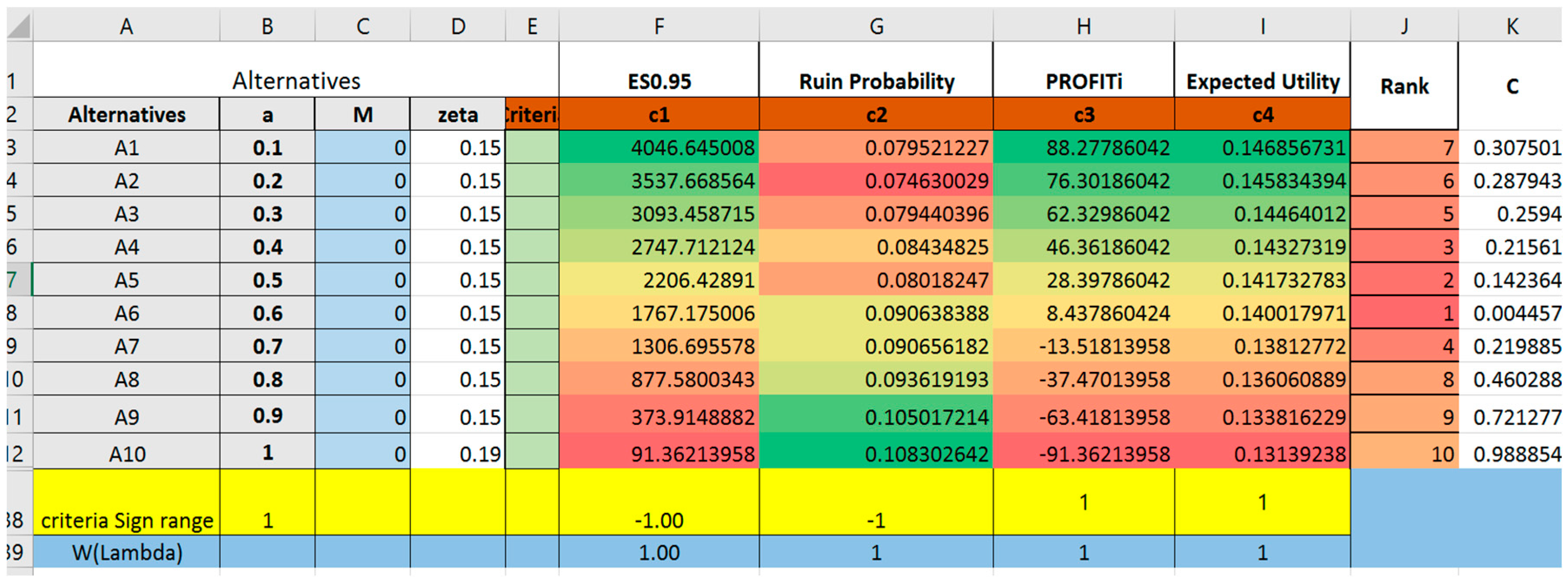
- In each trial, the Alternative 1 M = 0 simulates the scenario of pure proportional reinsurance. Trial 5 attempts to model different retention level under proportional reinsurance () with fixed reinsurance premium loading factor . The result shows that given same premium loading factor, retention level of 0.6 would be most preferable.
- By setting (a, M) to (0, 0), we could also model the scenario of no reinsurance. The results show that with no reinsurance, the expected shortfall of insurance company will be significantly higher than all other alternatives, and the ruin probability will be higher as well. This suggests that insurance company without reinsurance is more likely to become bankrupt if large losses are incurred. As compensation, the expected profit and utility will increase by a small amount for the insurance company due to high profit from insurance premium and low probability of large losses. However, noting the high ruin probability, which suggests a much higher risk of bankruptcy, the insurance company will often seek for reinsurance to keep ruin probability low.
- Furthermore, through the simulation process, the variance and profitability of the reinsurer are also being observed and calculated (as can be seen from Figure 9). The result was in correspondence with our previous argument that by scaling the ceding portion a to larger values, both the variance and the profitability of the reinsurer will increase, suggesting that there is a trade-off between high profit and high risk of large losses. Thus, this supports our previous assumption that the reinsurer is ambiguous towards a design that only differs with respect to parameter a.
6. Conclusions
6.1. Contributions
The research has the following contributions:
- To the best of our knowledge, this is the first theoretical study using MADM to approach proportional–stop-loss reinsurance model, though there are a few recent studies using MADM in designing either pure proportional or pure stop-loss reinsurance contracts;
- This is one of the few studies taking a non-discriminatory position considering both the insurance and the reinsurance company in designing an optimal reinsurance contract, and the study made significant contribution by incorporating existing MODM models and the promising MADM model into one decision flow process to arrive at a robust decision for reinsurance design;
- This study demonstrates the feasibility of incorporating intelligent decision supporting systems in reinsurance deal-making. As observed by the author through industry experiences, @Risk has grown its popularity recently for actuarial study in modeling risk and claims. The prototype of TOPSIS implemented through Matlab suggests that a software of multi-criteria decision support would be promising.
- As previous research suggested (Bazaz and Najafabadi 2015), MADM is not likely to address finding of optimal type of reinsurance. However, with the generic formulation of proportional–stop-loss reinsurance, we would be able to model proportional reinsurance and stop-loss reinsurance as special cases of proportional–stop-loss, thus the choice between proportional and non-proportional reinsurance using MADM could be possible under this formulation of reinsurance.
6.2. Limitations
There are still some limitations for this research, specifically in the following aspects:
- In terms of the scope of study, due to time and resource constraints the study only considers proportional-stop-loss treaty reinsurance, while basing the decision process on ruin probability, CVaR, and expected utility criteria. Other types of reinsurance and decision measurements have not been elaborated and tested.
- In terms of methodology, this study attempts to utilize the simulation software @Risk to model the loss and claim distribution and to use numerical TOPSIS model in modeling decisions from the insurance company, without reaching to a close-form solution. Thus, the conclusions were drawn based on simulation result rather than robust theoretical derivation.
- In terms of model implementation, due to resource constraints, this study only includes a numerical made-up case instead of existing cases to conduct archival research in addressing the decision process in the reinsurance purchase decisions.
6.3. Future Directions
In reality, trade contracts will usually go through lengthy negotiations with broking firms acting as intermediaries, thus, empirical study with cases from existing broking firms may be more realistic and practical in addressing the usefulness of this decision framework. In addition, behavioral study of both the reinsurer and the reinsured party would be of great importance to suggest whether they are rational players in the reinsurance market.
Furthermore, it would be promising for mathematical and quantitative researchers to look into the closed-form optimization for proportional–stop-Loss under each single measurement. As pure proportional or stop-loss reinsurance could be regarded as special cases of proportional–stop-loss reinsurance could, this will reconcile existing mathematical models on either side and help in calculating the precise decision matrix for MADM analysis.
Author Contributions
The authors contributed equally to the paper.
Conflicts of Interest
The authors declare no conflict of interest.
Appendix A. TOPSIS Trials #2, #3 and #4
Figure A1.
Trial 2: Screen-shot of crucial TOPSIS output parameters.

Figure A2.
Trial 2: Screen-shot of crucial TOPSIS output parameters.

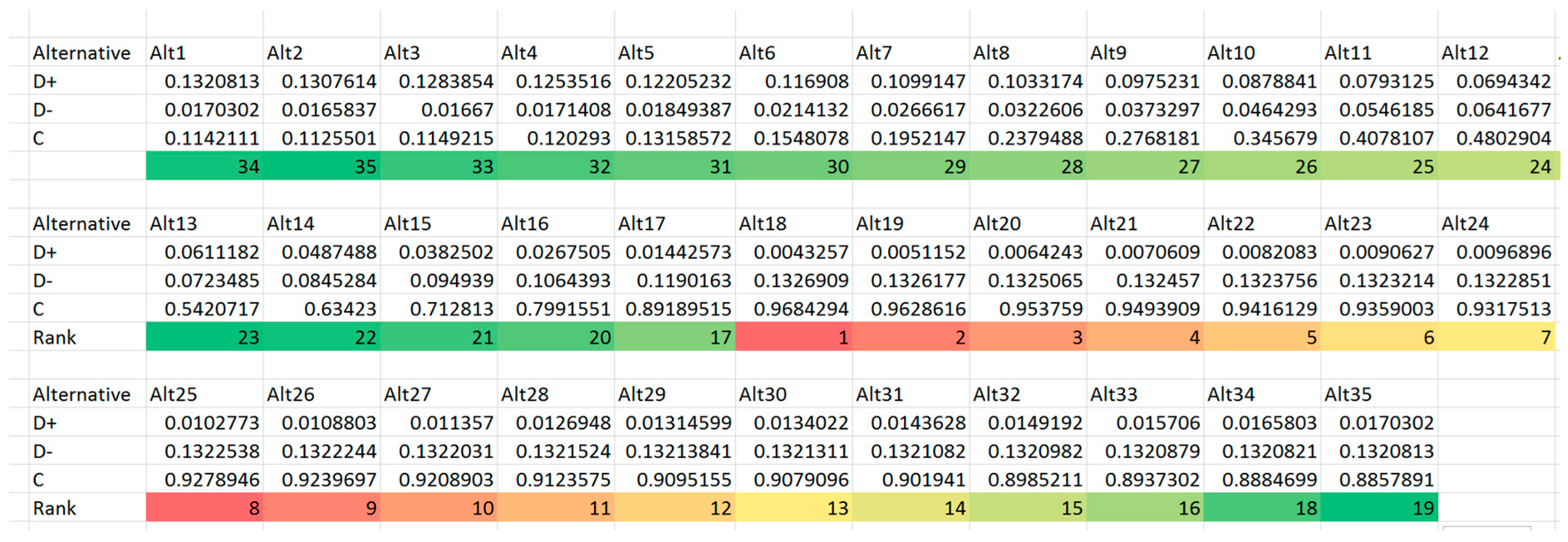
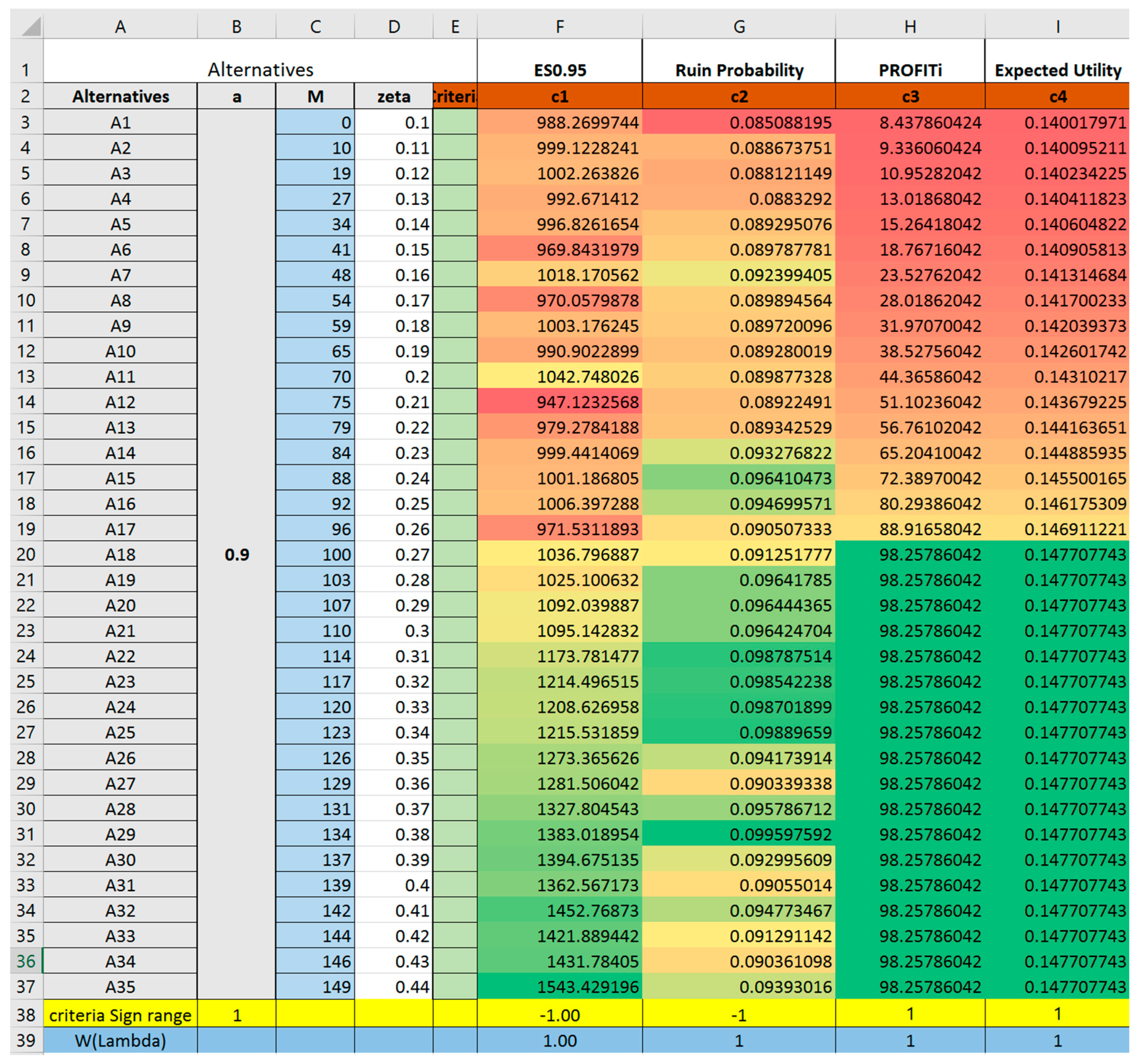
Figure A3.
Trial 3: Screen-shot of crucial TOPSIS output parameters.

Figure A4.
Trial 3: Screen-shot of crucial TOPSIS output parameters.

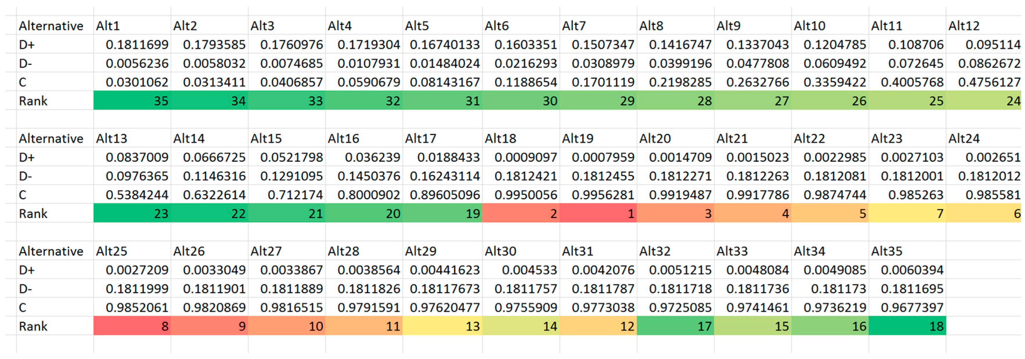
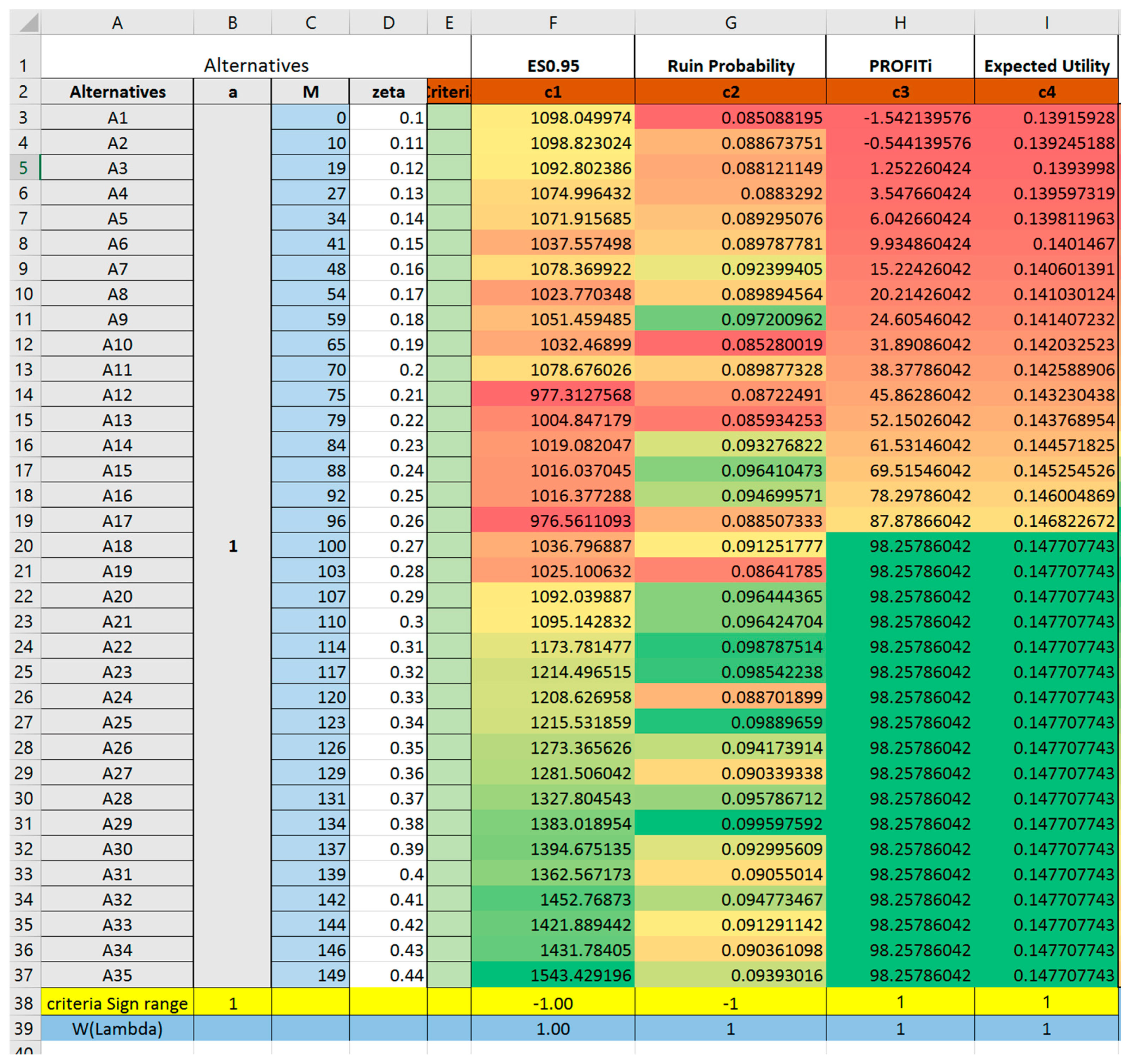
Figure A5.
Trial 4: Screen-shot of crucial TOPSIS output parameters.

Figure A6.
Trial 4: Screen-shot of crucial TOPSIS output parameters.

References
- Ameri Sianaki, Omid. 2015. Intelligent Decision Support System for Energy Management in Demand Response Programs and Residential and Industrial Sectors of the Smart Grid. Doctoral dissertation, Curtin University, Bentley, Western Australia, Australia. [Google Scholar]
- Bazaz, Ali Panahi, and Amir T Payandeh Najafabadi. 2015. An Optimal Reinsurance Contract from Insurer’s and Reinsurer’s Viewpoints. Applications & Applied Mathematics 10: 970–982. [Google Scholar]
- Borch, Karl. 1960. Reciprocal Reinsurance Treaties Seen as a Two-Person Co-Operative Game. Scandinavian Actuarial Journal 1960: 29–58. [Google Scholar] [CrossRef]
- Borck, Karl. 1960. An Attempt to Determine the Optimum Amount of Stop Loss Reinsurance. Brussels: Brussels, pp. 597–610. [Google Scholar]
- Cai, Jun, Haiyan Liu, and Ruodu Wang. 2017. Pareto-optimal reinsurance arrangements under general model settings. Insurance: Mathematics and Economics. [Google Scholar] [CrossRef]
- Carter, R. L. 1979. Reinsurance. Berlin: Springer. [Google Scholar]
- Chauhan, Aditya, and Rahul Vaish. 2013. Fluid Selection of Organic Rankine Cycle Using Decision Making Approach. Journal of Computational Engineering 2013. [Google Scholar] [CrossRef]
- Hürlimann, Werner. 2011. Optimal Reinsurance Revisited–point of View of Cedent and Reinsurer. Astin Bulletin 41: 547–74. [Google Scholar]
- Hwang, Ching-Lai, Young-Jou Lai, and Ting-Yun Liu. 1993. A new approach for multiple objective decision making. Computers and Operational Research 20: 889–99. [Google Scholar] [CrossRef]
- Hwang, Ching-Lai, and Kwangsun Yoon. 1981. Multiple Attribute Decision Making: Methods and Applications. New York: Springer. [Google Scholar]
- Karageyik, Başak Bulut, and David Dickson. 2016. Optimal reinsurance under multiple attribute decision making. Annals of Actuarial Science 10: 65–86. [Google Scholar] [CrossRef]
- Karageyik, Başak Bulut, and Şule Şahin. 2017. Determination of the Optimal Retention Level Based on Different Measures. Journal of Risk and Financial Management 10: 4. [Google Scholar] [CrossRef]
- Liang, Haiming. 2014. Research on Methods for Two-Sided Trade Matching Decision-Making Based on the Broker. Ph.D. Thesis, Northeastern University, Boston, MA, USA. [Google Scholar]
- Payandeh-Najafabadi, Amir T, and Ali Panahi-Bazaz. 2017. An Optimal Combination of Proportional and Stop-Loss Reinsurance Contracts from Insurer’s and Reinsurer’s Viewpoints. arXiv Preprint, arXiv:1701.05450. [Google Scholar]
- Samson, Danny, and Howard Thomas. 1983. Reinsurance Decision Making and Expected Utility. The Journal of Risk and Insurance 50: 249–64. [Google Scholar] [CrossRef]
- Samson, Danny, and Howard Thomas. 1985. Decision analysis models in reinsurance. European Journal of Operational Research 19: 201–11. [Google Scholar] [CrossRef]
- Vajda, Stefan. 1962. Minimum Variance Reinsurance. Astin Bulletin 2: 257–60. [Google Scholar] [CrossRef]
- Wang, Gang. 2003. Reinsurance Optimization Models. Ph.D. Thesis, Hunan University, Changsha, China. [Google Scholar]
- Yoon, Kwangsun. 1987. A reconciliation among discrete compromise situations. Journal of Operational Research Society 38: 277–86. [Google Scholar] [CrossRef]
Figure 1.
Trade procedure P1 (Liang 2014).
Figure 1.
Trade procedure P1 (Liang 2014).

Figure 2.
Trade procedure P2 (Liang 2014).
Figure 2.
Trade procedure P2 (Liang 2014).

Figure 3.
Graphical representation of technique for order of preference by similarity to ideal solution (TOPSIS) (Chauhan and Vaish 2013).
Figure 3.
Graphical representation of technique for order of preference by similarity to ideal solution (TOPSIS) (Chauhan and Vaish 2013).

Figure 4.
Case study flowchart in modeling real-world reinsurance deals.

Figure 5.
Optimal pairs of reinsurance design given constant ceding portion .

Figure 6.
Screenshot of criteria calculation using Monte Carlo simulation with @Risk.

Figure 7.
Construction of a decision matrix for preparation of TOPSIS.

Figure 8.
Ranking of the alternatives based on TOPSIS.

Figure 9.
Trial 5: Pure proportional reinsurance selection.


Table 1.
Key variable definitions.
| Variable | Variable Explanation |
|---|---|
| the time period of one contract, in our case study ; | |
| the number of claims incurred in period t (during one contract); | |
| the wealth held by insurance company at time t; | |
| the loading factor of the reinsurance premium paid to the reinsurer; | |
| the loading factor of the premium paid to the reinsured party; | |
| the claim amount of one single loss; | |
| the claim amount payable by the insurance company (the reinsured party); | |
| the claim amount payable by the reinsurance company (the reinsurer); | |
| the aggregate loss of an insurance portfolio; | |
| the aggregate claim (loss) incurred to insurance company (the reinsured party); | |
| the aggregate claim (loss) incurred to the reinsurance company (reinsurer); | |
| the cumulative distribution function of S; | |
| the survival distribution function of S; | |
| the proportional–stop-loss reinsurance parameter,; | |
| the total premium per unit time; | |
| the premium gained by the insurance company; | |
| the premium payable to the reinsurer; | |
| the expected shortfall with a confidence level of ; | |
| the expected profit gained by insurance company; | |
| the ruin probability of insurance company’s wealth ; | |
| the utility of insurance company at the end of period t; |
© 2017 by the authors. Licensee MDPI, Basel, Switzerland. This article is an open access article distributed under the terms and conditions of the Creative Commons Attribution (CC BY) license (http://creativecommons.org/licenses/by/4.0/).
Share and Cite
MDPI and ACS Style
Wang, S.J.X.; Poh, K.L. Intelligent Decision Support in Proportional–Stop-Loss Reinsurance Using Multiple Attribute Decision-Making (MADM). J. Risk Financial Manag. 2017, 10, 22. https://doi.org/10.3390/jrfm10040022
AMA Style
Wang SJX, Poh KL. Intelligent Decision Support in Proportional–Stop-Loss Reinsurance Using Multiple Attribute Decision-Making (MADM). Journal of Risk and Financial Management. 2017; 10(4):22. https://doi.org/10.3390/jrfm10040022
Chicago/Turabian StyleWang, Shirley Jie Xuan, and Kim Leng Poh. 2017. "Intelligent Decision Support in Proportional–Stop-Loss Reinsurance Using Multiple Attribute Decision-Making (MADM)" Journal of Risk and Financial Management 10, no. 4: 22. https://doi.org/10.3390/jrfm10040022