Surf Zone Turbulence and Suspended Sediment Dynamics—A Review

Abstract

The existence of sandy beaches relies on the onshore transport of sand by waves during post-storm conditions. Most operational sediment transport models employ wave-averaged terms, and/or the instantaneous cross-shore velocity signal, but the models often fail in predictions of the onshore-directed transport rates. An important reason is that they rarely consider the phase relationships between wave orbital velocity and the suspended sediment concentration. This relationship depends on the intra-wave structure of the bed shear stress and hence on the timing and magnitude of turbulence production in the water column. This paper provides an up-to-date review of recent experimental advances on intra-wave turbulence characteristics, sediment mobilization, and suspended sediment transport in laboratory and natural surf zones. Experimental results generally show that peaks in the suspended sediment concentration are shifted forward on the wave phase with increasing turbulence levels and instantaneous near-bed sediment concentration scales with instantaneous turbulent kinetic energy. The magnitude and intra-wave phase of turbulence production and sediment concentration are shown to depend on wave (breaker) type, seabed configuration, and relative wave height, which opens up the possibility of more robust predictions of transport rates for different wave and beach conditions.

1. Introduction

The coexistence and interaction of hydrodynamic motions over a wide range of timescales create a rather chaotic surf zone environment. Incoming wind waves and swell operate across a broad spectrum of frequencies, they shoal and break, and they generate time-averaged cross- and longshore currents, long-period infragravity waves, as well as turbulence that emanates from both the sea surface and from the seabed. While surf zone processes can often be described in a deterministic manner, many of the processes interact in complex and sometimes non-linear ways with each other and the seabed, making it challenging to describe aspects of the system other than stochastically. Consequently, detailed model simulations and accurate predictions are difficult. For example, the theoretical foundations for the process of wave breaking are still weak, and the role of surface-generated turbulence on vertical and horizontal mixing and sediment mobilization is not well understood for natural situations.

When surface gravity waves propagate into shallow water, wave energy is dissipated and momentum is transferred into the bottom boundary layer by friction between the fluid and the seabed. Further landward, the waves break in the outer surf zone; the free stream flow changes from (nearly) irrotational to rotational and vortices generated by wave breaking transfer momentum into the water column, sometimes reaching into the bottom boundary layer and affecting the seabed. The force per unit area that the fluid exerts on the sediment bed is the bed shear stress (τ_b). It mobilizes sediment grains and causes them to roll, slide, or saltate along the bed as bedload. With increasing stress, particles collide in the bed layer and some particles may gain sufficient vertical momentum to be suspended in the water column. Alternatively, sediment may be suspended through flow separation around seabed irregularities such as wave ripples, or when upward-directed pressure components within the bed induced by fluid turbulence become so large that the resulting upward force is sufficient for the particles to rise and detach from the bed [1]. This is the case, for example, when breaking-wave generated vortices induce large upward-directed pressure gradients in the seabed [2]. Because wave boundary layers are much thinner than boundary layers associated with time-averaged mean currents, wave-generated bed shear stresses are significantly larger than current-derived stresses. Understanding of the temporal variation of wave-generated τ_b is therefore essential for the prediction of sediment transport under wave motion [3].

Numerical models for nearshore sediment transport are typically underpinned by three assumptions: (i) Sediment is mobilized at the fluid/bed interface by small-scale turbulence generated by shear between the fluid and the seabed. (ii) Consequently, τ_b scales with the horizontal wave orbital velocity (u) and it is in phase with u, and (iii) the sediment load (bedload and suspended load) scales with τ_b. Therefore, net sediment transport, q, also scales with τ_b, $q\propto \left|u{\tau }_b\right|$. However, as pointed out by Foster et al. [4], because τ_b is unknown in most cases, the models often rely on simple quadratic assumptions (stress scales with velocity-squared) or eddy viscosity models to describe shear stress and sediment load.

Present-day operational sediment transport models typically predict sediment transport due to time-averaged flows quite well, also under breaking-wave conditions. Time-averaged sediment load indeed does tend to scale with shear stress, mean current speeds are, if not trivial, then relatively simple to simulate with some accuracy, and a mean (current-driven) sediment transport is not reliant on time-dependencies. However, the models encounter significant difficulties with predicting oscillatory transport due to wave motions [5,6,7], which is not ideal since this is the most important mechanism for onshore sediment transport involved in beach recovery. In contrast to mean transport, oscillatory transport is time-dependent and must be resolved on intra-wave scale, and intra-wave quantities such as turbulence and bed shear stress are not well defined in most models. More detailed and sophisticated but computationally demanding single-phase RANS-based approaches do exist [8] and these models can resolve flow, turbulence, and sediment transport over wave phase (e.g., the SedWaveFoam two-phase model for sheet flow; [9]) but they have only been applied and tested for nonbreaking waves outside the surf zone. In general, numerical models assume that turbulent shear stresses derive from friction between the (horizontal) oscillatory flow and the seabed, and sediment load and transport therefore scale with higher order moments of u(t). Other sources of bed shear stress, for example, turbulence generated by surface wave breaking are typically not included and presently available models are not, therefore, particularly well-suited for simulation of surf zone sediment transport.

Longo et al. [10] reviewed surf zone turbulence and Sumer and Fuhrman [11] (their chapter 7) recently published an exhaustive treatment of turbulence in coastal waters, while aspects of nearshore sediment transport were reviewed, for example, by Aagaard and Hughes [12]. The present paper aims to provide an up-to-date review of recent experimental advances on turbulence characteristics and generation in the surf zone and its effects on sediment mobilization, suspended sediment load, and wave-driven (i.e., time-dependent) suspended sediment transport. The focus is mainly on intra-wave properties due to their significance to (peak) bed shear stresses and onshore sediment transport, and the review is mainly concerned with experimental results rather than with numerical model simulations. Following this introduction (1), we discuss the following themes: (2) the definition and parameterization of shear stress and its relation to turbulent quantities; (3) current methods to measure turbulence under waves with a particular focus on field conditions; (4) a review of turbulence generation and its spatio-temporal structure with emphasis on surface-generated turbulence in the surf zone; (5) the effect of turbulence on sediment mobilization and sediment concentrations; (6) the intra-wave properties of turbulent kinetic energy production and sediment suspension under wind waves, again with an emphasis on conditions within the surf zone; (7) wave-driven sediment transport as affected by turbulence, its magnitude, and timing within the wave cycle; and finally (8), a summary and discussion of future perspectives in empirical studies and modeling of turbulence and sediment transport.

2. Bed Shear Stress

Bed shear stress is defined as the tangential force that the fluid exerts on the seabed per unit area. While the bed shear stress can rarely be measured directly, various methods exist for its estimation and parameterization [13,14]. The classic expression for τ_b is based on the log-law derived from unidirectional flows:

$$\frac{u}{u_{*}}=\frac{1}{\kappa }\ln \frac{z}{z_0}$$

(1)

where $u_{*}$ is the friction velocity, κ is the von Karman constant, z is the elevation (within, or at the top of the boundary layer) at which the two-dimensional horizontal fluid velocity vector, u, is specified and z₀ is the hydraulic bed roughness. Measuring the horizontal velocity profile within the boundary layer provides an estimate of $u_{*}$, and $u_{*}$ is related to shear stress through

$${\tau }_b=\rho u_{*}\left|u_{*}\right|$$

(2)

where ρ is fluid density. Due to the unsteady nature of oscillatory flow under waves, the wave boundary layer is typically thin, in the order of a few centimeters, and estimating the friction velocity from a measured velocity profile using (1) and (2) is generally difficult, especially in the field where highly energetic conditions prevent the use of fragile high-resolution instruments. Alternatively, shear stress (τ) can be estimated from a point measurement of the Reynolds stress associated with fluid shear (sometimes termed the velocity covariance method):

$$\tau =-\rho \langle u^{\prime }{w}^{\prime }\rangle$$

(3)

where w is vertical velocity, primes denote turbulent quantities, and the brackets indicate time-averages. To obtain the bed shear stress from Equation (3), the turbulent velocities must be measured at a point within a constant stress layer near the bed. Reynolds stress estimates include only the coherent part of the turbulence and are not always simple to obtain because of potential errors associated with sensor misalignment relative to the axes of the flow. Further, the assumption of constant stress may be difficult to justify in accelerating/decelerating wave-driven flows.

Shear stress can also be estimated from measurements of turbulent kinetic energy (TKE; [15,16]):

$$\tau =C\rho k$$

(4)

where C is a constant in the order of 0.2, and k is turbulent kinetic energy per unit mass, k = 0.5(<u′²> + <v′²> + <w′²>), where v is the transverse velocity component. Kim et al. [13] and Pieterse et al. [14] evaluated Equations (2)–(4) and both found that the TKE method yielded the most consistent results of τ, although more work is required to determine the magnitude of the constant of proportionality, especially under wave-driven flows.

A fourth way of estimating turbulence and (bed) shear stress is through estimation of the turbulent dissipation (ε) using, for example, the velocity frequency spectrum. This approach requires the assumption that turbulent production and dissipation are balanced everywhere, as well as application of Taylor’s hypothesis of frozen turbulence. The latter relates the turbulent length scale to turbulent frequency within the inertial subrange (e.g., [17]):

$$E\left(f\right)=\frac{\alpha }{2{\pi }^{2/3}}{u}^{2/3}{\epsilon }^{2/3}{f}^{5/3}$$

(5)

where α is the Kolmogorov constant (≈0.65), ε is the turbulent dissipation rate (defined as ε = −<u′w′> du/dz; [18]), and E(f) is the spectral density at frequency f. The assumption is made that turbulent vortices are advected by currents (or ‘long’ waves) past the point of measurement, but the criteria for its use, namely that u >> u′ and u >> Δu (where Δu is the variation of u over the turbulent length scale) are often grossly violated in the field [19].

3. Turbulence Measurement

Turbulent velocities under waves can be measured with a range of different instruments. Hot-film sensors, Laser Doppler Anemometers (LDA; [20,21]), and Particle Image Velocimetry (PIV; [22,23,24]) have all found favor in laboratory settings where they can provide detailed and precise measurements. However, these instruments are all quite fragile and measure velocities in only two dimensions. That may not be a critical issue in laboratory wave flumes, but it certainly is in surf zone field experiments where waves are directionally spread and strong currents may be oriented perpendicularly to the incoming waves. In field settings, more robust—but often perhaps less accurate—instruments are used routinely for turbulent measurement such as 3D acoustic Doppler velocimeters (ADV), which may be mounted in vertical arrays (e.g., [25]), acoustic Doppler profilers (ADP; [26,27]), or electromagnetic current meters ([28]).

Both the Reynolds-stress (Equation (3)) and TKE (Equation (4)) methods for estimating stress rely on isolation of turbulent quantities from the total flow vector(s), which may be less than straightforward in wave-driven oscillatory flows. The instantaneous velocity field can be resolved into three components:

$$\begin{gathered} u=\overline{u}+\tilde{u}+u^{\prime } \\ \mathrm{and} \\ w=\overline{w}+\tilde{w}+w^{\prime } \end{gathered}$$

(6)

where overbars indicate mean components, tildes represent the oscillatory flow, and primes are turbulent quantities. While it is trivial to subtract the mean from a time-series, separation of oscillatory and turbulent components is less so, partly because they often overlap in frequency space (e.g., [28,29]).

For regular waves, a common way to remove the wave component is to use ensemble averaging (e.g., [21,30]) by calculating the quantity:

$$\overline{X}(t)=\frac{1}{N}{\displaystyle \sum _{n=0}^{N-1}X(t+nT)}$$

(7)

where X represents the variable in question, in this case u or w, t represents time, T is wave period, and N is the number of ensembles. The turbulence component is calculated as the residual between the velocity time-series and the ensemble-averaged product. However, since waves are rarely regular in nature, other techniques must be used here, for example frequency cut-off methods, involving high-pass filtering to isolate turbulence. Thornton [31] calculated the co-spectrum between u and surface elevation (η) to identify the frequency limit between wave motion and turbulence. This method turned out to be less useful as large turbulent vortices do impose a surface signal [32].

Alternatively, horizontal/vertical velocity spectral cut-offs have been defined on the basis of breaks in spectral slope within the high-frequency part of the spectrum (e.g., [4,33,34]). Surface wave energy should decay as f⁻³ and the inertial subrange is expected to exhibit a spectral decay of f^−5/3 under the assumption that Taylor’s hypothesis of frozen turbulence (Equation (5)) applies.

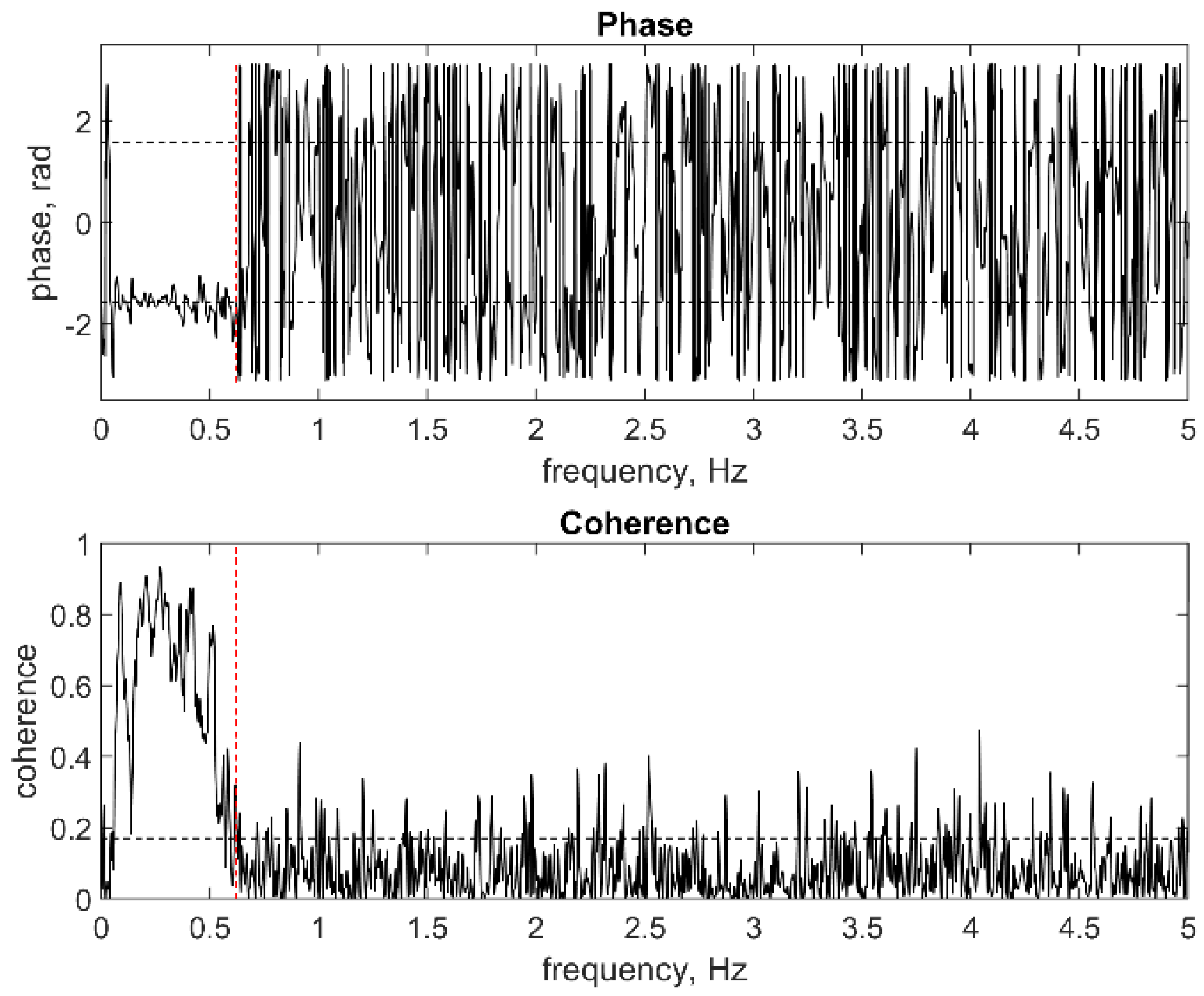
Christensen et al. [35] introduced a modified frequency cut-off method using the co-spectral phase between u and w to define the frequency that separates wave orbital motion from turbulent motion. For wave orbital motions outside the wave boundary layer, the phase between u and w is expected to be ±π/2 and with statistically significant coherence, whereas for turbulence, the u-w phase is expected to exhibit continuous and erratic phase jumps with low coherence. Figure 1 shows an example of the u-w co-spectral technique, where the transition from dominance of wave orbital motion to turbulence (the cut-off frequency) was estimated at f = 0.62 Hz, based on the u-w phase jumps and the drop to statistically insignificant coherence. It is clear, however, that such imposed cut-off frequencies do not uniquely define, for example, the gravity wave and turbulence frequency bands since gravity wave motion may leak into frequencies above the cut-off, and large-scale turbulent motions may exist at frequencies below the cut-off such that an overlap region must be expected. However, the cut-off should identify the spectral bandwidths where the respective motions (wave orbital vs. turbulent) are dominant [36].

Alternatively, Bricker and Monismith [37] devised a phase-method operating in the spectral domain that produced satisfactory results in cases when the wave-induced strain field was weaker than the turbulence strain field. However, recently a standard method has emerged where two or more velocity sensors are deployed, separated in either the vertical or the horizontal dimension. This velocity-differencing method is based on work by Trowbridge [38], which was later extended by [39,40]. The method relies on the assumption that a turbulence decorrelation length scale exists and that correlations between two sensors separated in space will include wave, but not turbulence components; hence, wave bias in the time series can be removed. As a check on Reynolds-stress estimates derived from this method, Feddersen and Williams [40] introduced the non-dimensional integrated co-spectrum Og_u′w′(f) (the ogive curve) for u′w′, which was defined as

$$O{g}_{u^{\prime }{w}^{\prime }}(f)={\displaystyle \underset{f}{\int }\frac{C{o}_{u^{\prime }{w}^{\prime }}(f)df}{\overline{u^{\prime }{w}^{\prime }}}}$$

(8)

where Co_u′w′ is the co-spectrum of u′w′. When co-spectral wave bias is minimal, ogive curves are expected to increase gently from 0 to 1 over a wide frequency range [41]. On the other hand, if the curves increase sharply over a narrow frequency range, or fluctuate erratically with frequency, the stress estimates are likely wave-bias contaminated. However, a robust test to reject bad Reynolds stress estimates does not yet exist [25].

Feddersen and Williams [40] concluded that the velocity-differencing technique appears to work well in the presence of strong currents. That would imply that it may be most suitable for estimating turbulence in the longshore dimension where the oscillatory velocity component is relatively weak, while, on the other hand, turbulence estimates may contain wave bias in cases when currents are relatively weak. A further question mark relating to this technique is the uncertainty with respect to the optimal sensor separation distance; Brinkkemper et al. [42] found that turbulence magnitudes increased with sensor separation. In addition, it is unclear if, and how, a potential optimum separation distance might change with wave conditions.

Christensen et al. [35] evaluated the u-w co-spectral technique relative to the velocity-differencing method and found that turbulent kinetic energy (k) estimated by the u-w method was about a factor 2 smaller than estimates from velocity-differencing. The simplest explanation would seem to be that the former may tend to exclude large turbulent eddies with low frequencies [34,43], and/or that the latter may contain wave bias related to uncertainties with respect to optimum sensor separation distance. Importantly, however, the k-profiles, and the temporal variation of k within the time series were qualitatively similar using the two methods.

4. Turbulence Generation, Spatial Structure, and Magnitude

When waves are breaking in a surf zone, turbulence may be generated in several ways: through fluid shear, through flow separation around roughness elements, and by injection of turbulent kinetic energy from breaking waves. Over a smooth seabed, turbulence starts to appear in the boundary layer flow when the Reynolds number Re > 1.5 × 10⁵ (Re = Au/ν, where A is orbital amplitude and ν is kinematic viscosity) but this number is expected to be smaller for rough beds [11] (p. 260). Shear between the flow and the seabed creates micro-turbulent vortices such as vortex tubes and turbulent spots (e.g., [44,45]) that originate at the bottom boundary and spread upward through diffusion. Horizontal flow velocity and turbulent production are more or less in-phase and production of k scales with u² [46]. When incoming waves are skewed, maximum k-production therefore occurs under the wave crest [23]. In the field, the situation is rarely that simple because strong mean currents and/or infragravity waves may distort the in-phase relationship between u and k [47]. For example, a strong seaward directed undertow may enhance trough velocities to an extent where maximum k (and thus bed shear stress) occurs under the wave trough.

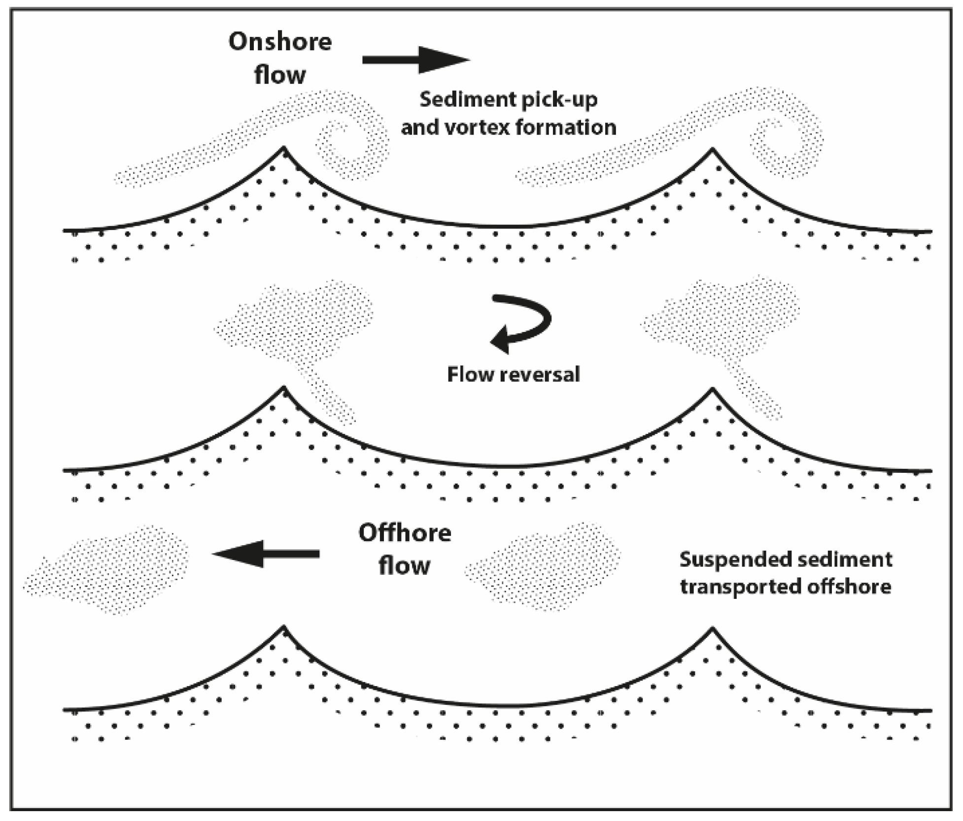
Bedforms, such as wave/current ripples, or megaripples may appear both outside and inside the surf zone, although ripples begin to decay when the mobility number $\psi =u^2/((s-1)gD$ > ≈200 (e.g., [48,49]), where (s − 1) denotes the relative sediment density, g is the acceleration of gravity, and D is the mean sediment grain size. When ripples are of moderate or large steepness, they often create flow separation and vortex shedding, as schematized in Figure 2. Turbulent vortices are generated on the lee slope of ripples during onshore and offshore wave phases and are ejected at flow reversals when the horizontal velocity is zero. In these coherent vortices, turbulence spreads upward by convection, rather than through diffusion [50]. Experimental evidence [51] and RANS modeling [52] have shown that vortex ejection enhances near-bed k and amplifies TKE to a level of about 4–8 ripple heights, in the model example corresponding to 25 cm above the bed.

Turbulent production caused by flow separation around bedforms scales with u and with bed roughness, with the latter depending on both sediment grain size and bedform steepness [50] and/or bedform height [54]. For skewed, shoaling waves, the production of k is maximum at the onshore-to-offshore flow reversal [55] such that u and k are in quadrature, as illustrated in Figure 2.

These two mechanisms for turbulent kinetic energy production may be relevant anywhere under wave motion, and an important added source appears within the surf zone where surface-generated turbulence due to wave breaking may become the dominant source of TKE, even close to the seabed [30,56]. Wave breaking is characterized by a sudden transition from irrotational to rotational flow, accompanied by a violent transformation of wave energy into turbulence and eventually heat [57,58]. Large-scale coherent vortices create strong vertical mixing, and surface-generated breaker turbulence spreads downward by convection [59]; however, in general, a relatively small part of the wave energy is dissipated below trough level with the majority being dissipated between wave crest and wave trough [60,61]. The relative wave height γ (γ = H/h, where H is wave height and h is water depth) is a useful parameter for characterizing, or scaling, a range of surf zone processes; for example, γ is used to predict the onset of wave breaking and breaking intensity, and wave energy dissipation scales with γ. If the relative wave height is sufficiently large (γ > ≈0.4; [62]), breaker turbulence may invade the wave boundary layer and hit the seabed [63].

Since surface- and bottom-generated turbulence coexist within the surf zone and generate turbulence at different wave phases (as will be discussed in Section 6), it is often useful to distinguish and separate the different sources of turbulence. Ruessink [25] argued that when surface-generated turbulence is dominant, the time-averaged turbulent momentum flux (ρ<u′w′>) should be predominantly negative (downward-directed) since vortices carry high-speed fluid towards the bed [64]. On the other hand, the net momentum flux may be expected to be positive when bottom-generated turbulence is dominant [21].

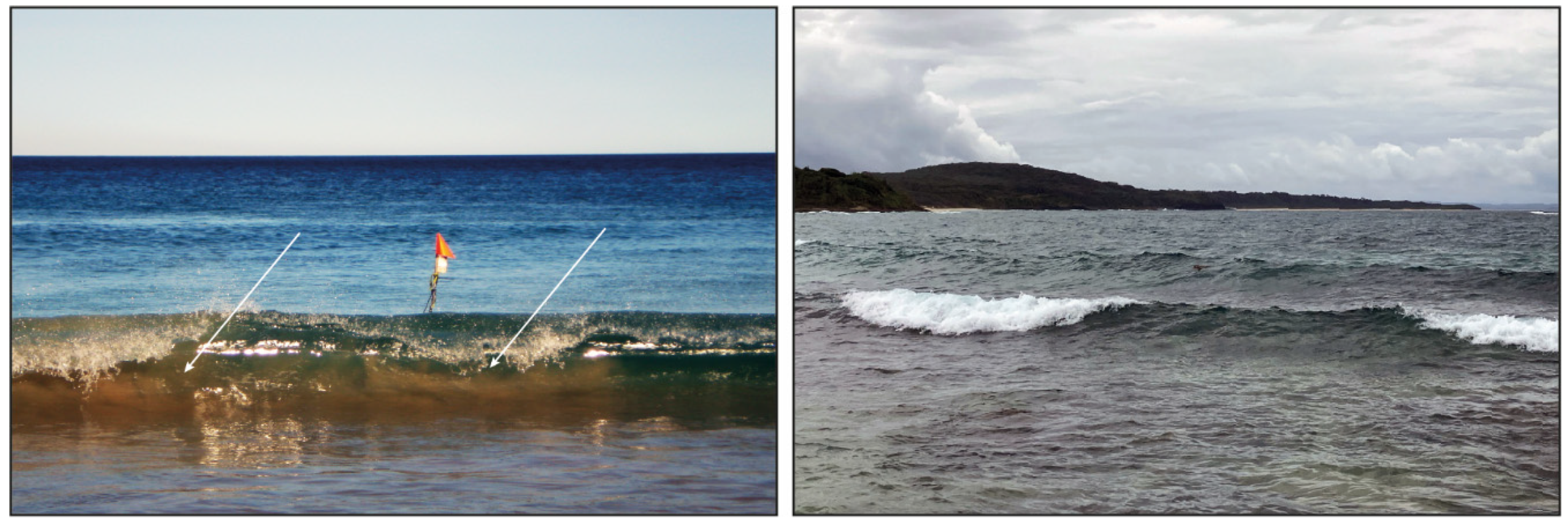
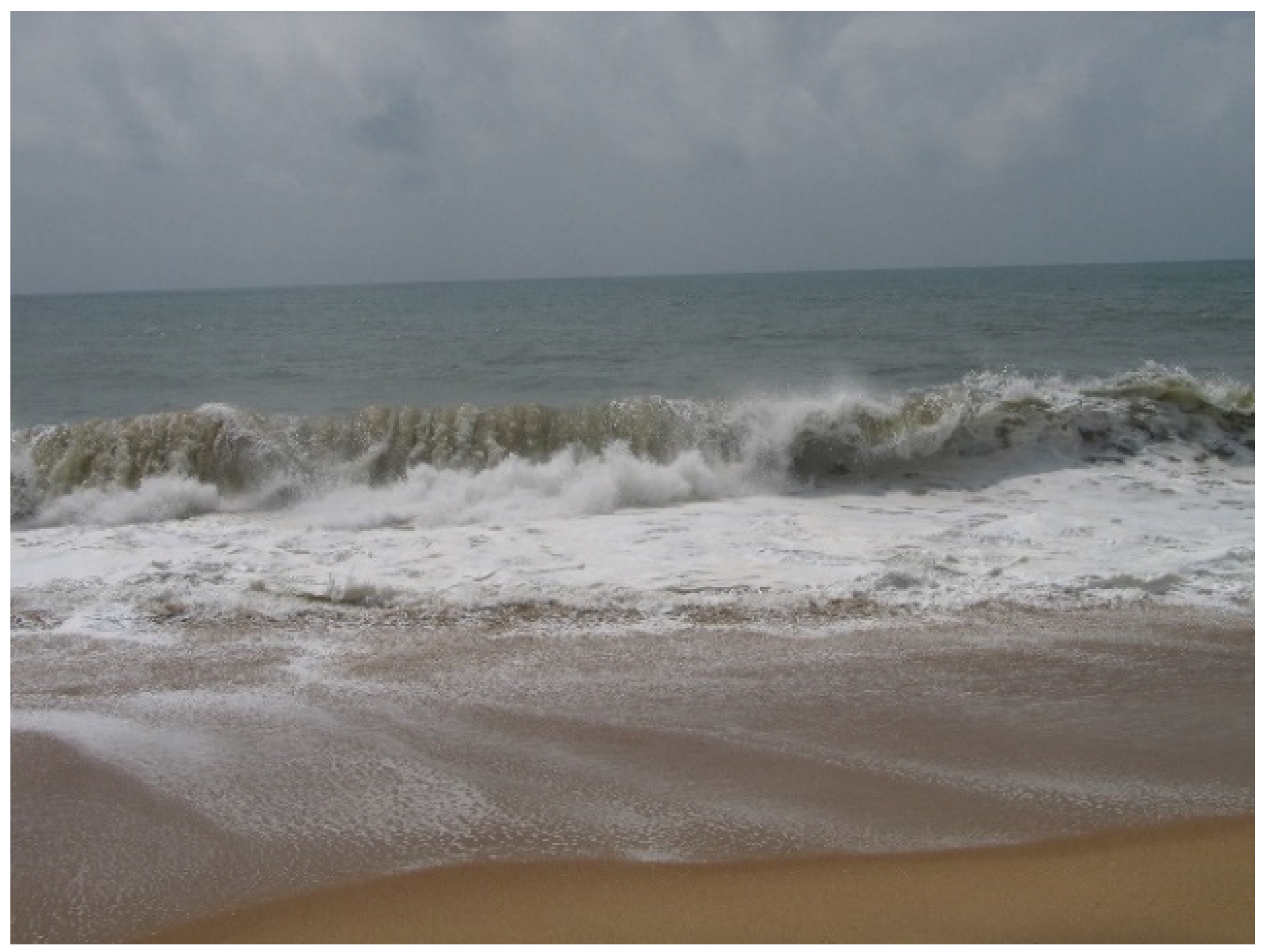
While wave breaking is a major turbulent source in the surf zone, the process is best described as stochastic. In an irregular wave field, some waves break while some do not. Turbulence production (and dissipation) is therefore highly intermittent, and instantaneous k-levels may be several orders of magnitude larger than wave-phase-averaged <k> [30]. Moreover, different types of wave breaking exist and the scale and intensity of the turbulent vortices depend on breaker type. In the outer surf zone, waves break through plunging or spilling (Figure 3). Both breaker types gradually transition into depth-saturated surf bores and this transition constitutes the limit between the outer and inner surf zones [65]. Sometimes it may be useful to distinguish these different wave types, and Grasso et al. [66] suggested that breakers and surf bores may be separated on account of the ratio between wave skewness and wave asymmetry.

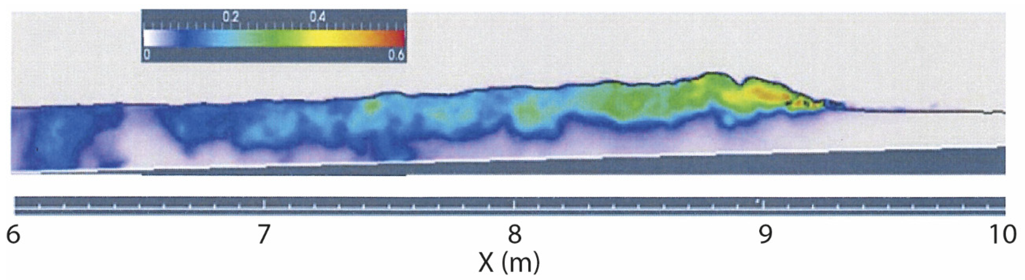
When breakers are spilling, turbulence spreads downward towards the seabed behind the wave crest. The process was probably initially described by Nadaoka et al. [32] who coined the turbulent structures ‘obliquely-descending eddies’ (ODEs) that trail behind the wave crest. They were also observed in laboratory experiments with surf bores [67], and Zhou et al. [68] visualized them numerically using a 3D Large Eddy Simulation Model (LES), see Figure 4. This figure shows that turbulence is created at the front of the wave and it spreads slowly downward towards the bed via descending eddies. The coherent turbulent structures impinge onto the bed as spatially isolated events some distance behind the wave crest.

When waves break through plunging, turbulence penetrates deeper into the bottom region than for spilling breakers, and the turbulent mixing rate below trough level is much larger [57]. Plunging breakers create large vortices, or downbursts, that rotate about a horizontal axis parallel to the wave crest [10,30] and generate oscillations in the vertical velocity [69] which may sometimes produce scour holes on the seabed [70]. In the field, Aagaard and Hughes [28] observed instantaneous velocities up to w ≈ 1 ms⁻¹ at an elevation 15 cm above the bed, and w_rms was about a factor 2 larger for plunging compared to spilling breakers of the same height, while deSerio and Mossa [71] reported that u′ was a factor 3 larger for plunging compared to spilling breakers.

Turbulent kinetic energy may be non-dimensionalized using Froude-scaling, $k^{\prime }=\left(\sqrt{k/gh}\right)$ which makes intuitive sense because the rate of turbulence production should scale with wave celerity [59]. For irregular waves in field and large-scale laboratory settings, <k′> ≈ 0.02–0.06 [42,72,73] which is typically smaller than for regular laboratory waves of similar root-mean-square height [25,56]. The difference arises because each regular wave injects turbulence while only some waves are breaking in an irregular wave field. <k′> has been observed to scale with γ [25,42] which is also consistent with expectations since turbulent production from wave breaking must scale with the intensity of wave breaking, and γ is a proxy for that intensity.

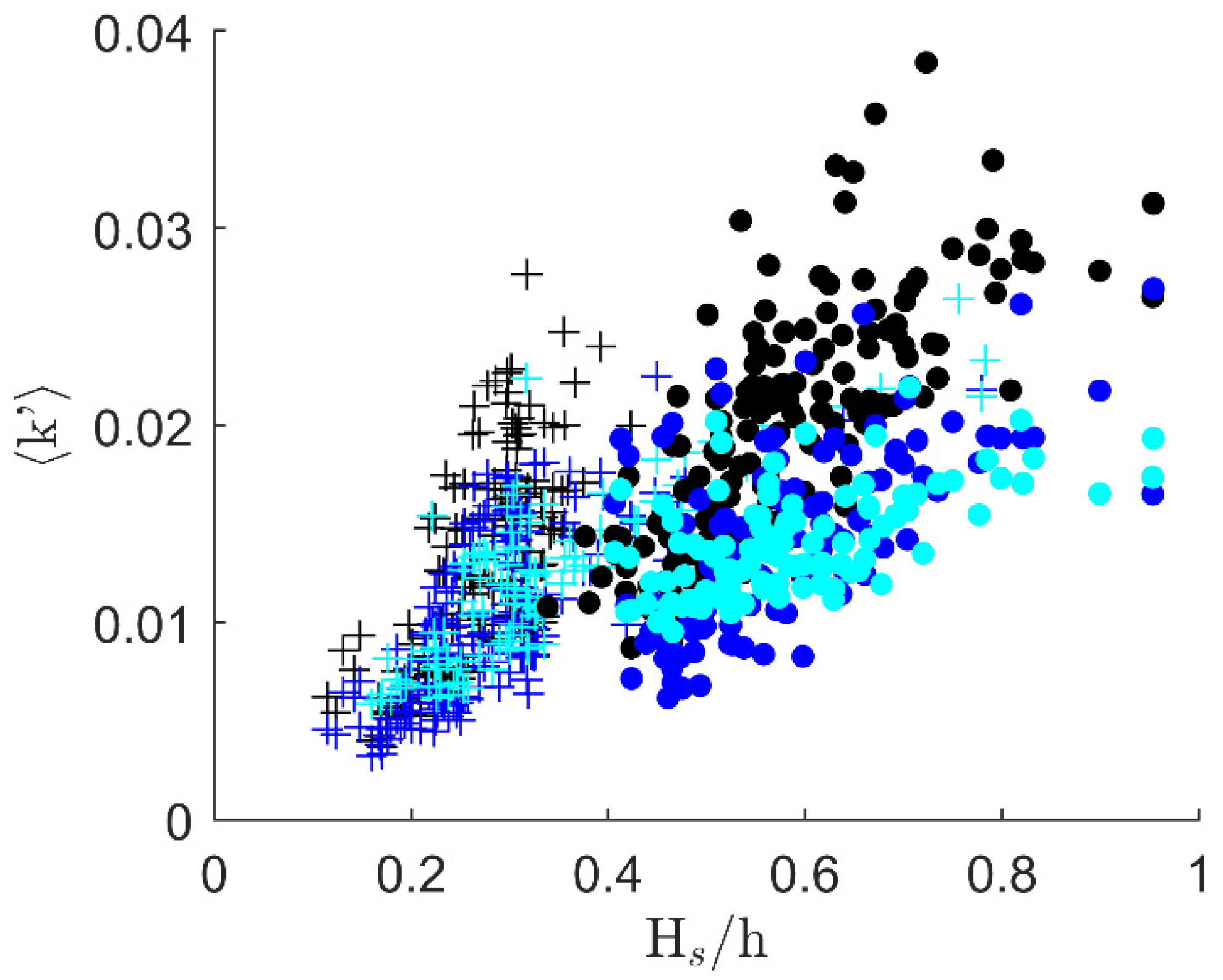
Christensen et al. [74] measured the turbulent kinetic energy at two beaches dominated by plunging breakers (Durras Beach, NSW, Australia, which is exposed to swell waves) and spilling breakers (Vejers Beach, Denmark, exposed to mainly wind waves). <k′> scaled with γ at both beaches (Figure 5) but with a significant degree of scatter, which is partly due to the different measurement elevations in the water column and uncontrollable bed level changes within and between periods of recording.

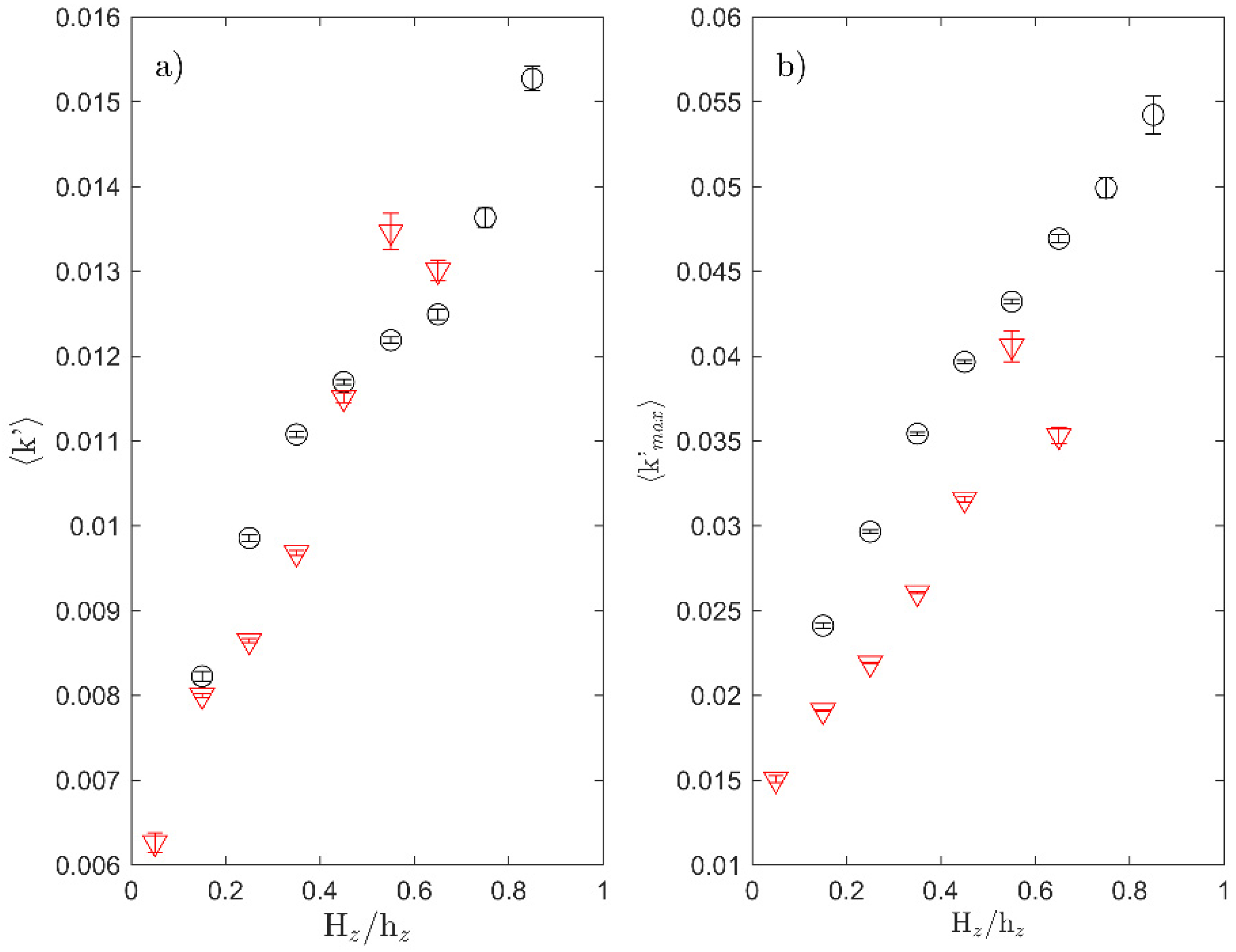
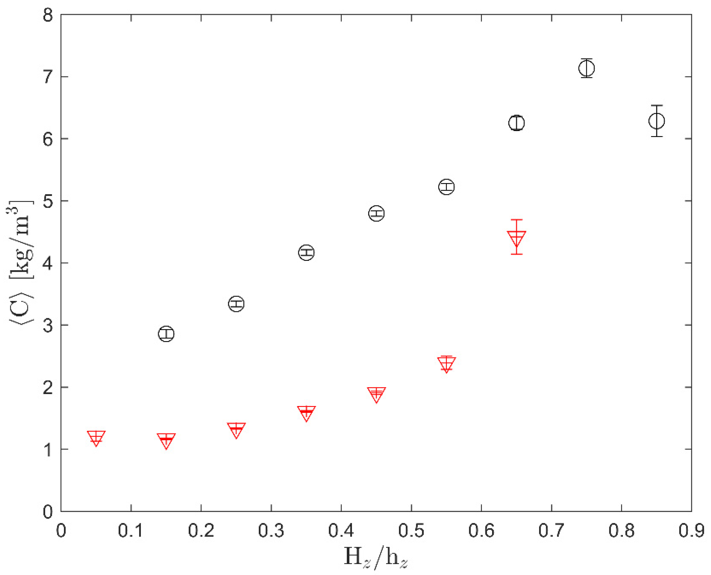
A different perspective is offered in Figure 6a. Here, data from roughly 60,000 waves were extracted from about 500 irregular-wave time series using a zero-downcrossing algorithm; the crest-to-trough height (H_z), mean water depth (h_z), and k were calculated for each wave and turbulence data were then binned within γ_z-ranges. Wave-averaged <k′> was similar at the two beaches (for similar γ) and scaled with the relative wave height, but maximum k′ during individual wave cycles (k′_max) were larger for plunging waves than for spilling (Figure 6b), which indicates that instantaneous levels of k are larger, but of shorter duration for plunging waves. This is consistent with Hsu et al. [73] who noted that for plunging breakers, instantaneous k(t) is typically many times larger than mean and phase-averaged <k>, while k may be up to a factor 5 larger for plunging breakers compared to shoaling waves [63].

Turbulent kinetic energy is related to eddy viscosity through

$$\sqrt{k}={\nu }_t/l$$

(9)

where ν_t is the eddy viscosity and l is a turbulent length scale. Eddy viscosity is often used in model simulations to describe sediment pick-up and the shape of the suspended sediment concentration profile, and the turbulent length scale expresses a distance over which the turbulent velocity becomes decorrelated; in other words, the length scale of the turbulent vortices. Measurements suggest that l = 0.1–0.3 h under breaking waves in the field [19,22,75,76] but l would be expected to depend on both breaker type as well as relative wave height. For plunging breakers, Aagaard and Jensen [77] calculated significantly larger turbulent length scales, l up to ≈ 0.65 h.

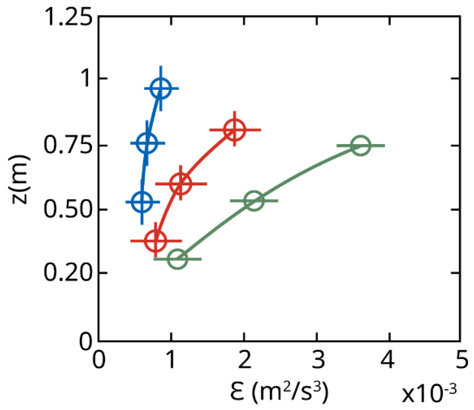
Time-averaged turbulence (<k>) tends to exhibit vertical structure within the water column, and the structure depends on location within (or outside) the surf zone. In general, observations have shown that for non-breaking waves, <k> is maximum at the bed. For breaking waves, Figure 7 illustrates some generally observed tendencies. The data were obtained from field measurements of the turbulent dissipation rate at Truc Vert beach [66] and show that for breaking waves, ε was almost uniformly distributed in the vertical, with a slight increase towards the upper parts of the water column. This is consistent with other field and laboratory experiments that have documented that plunging breakers, in particular, produce a very well-mixed water column with an almost uniform vertical distribution of <k> [25,78,79]. For surf bores in the inner surf zone, the field data in Figure 7 show a large decrease of ε towards the seabed.

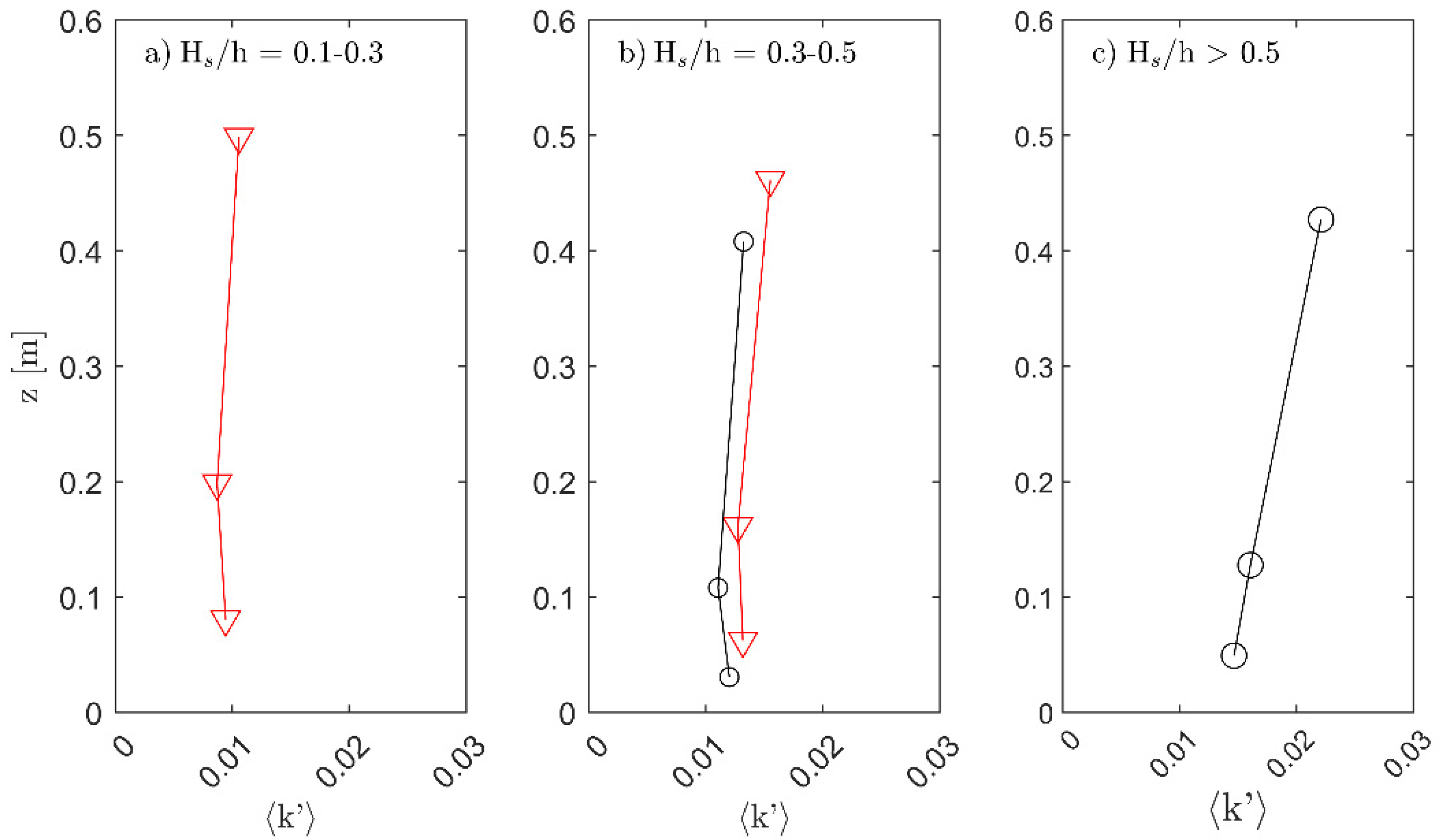
To illustrate near-bed tendencies in more detail, Figure 8 plots <k′>-profiles from two field experiments [74]. For strongly breaking wave conditions (γ_s = H_s/h > 0.5), <k′> was maximum at the highest measurement position (z = 50 cm) with a decrease of about 30% close to the bed (z ≈ 5 cm). For nonbreaking wave conditions (γ_s = H_s/h < 0.3), <k′> increased towards the bed due to the roughness created by small (mainly anorbital) wave ripples in fine-grained sand and <k′> was similar at the top and the bottom of the water column. Weakly breaking waves (0.3 < H_s/h < 0.5) exhibited a mixture of the two shapes with <k′> being largest at the highest measurement elevation and likely even larger near the sea surface.

The vertical turbulence structure depends not only on the relative wave height but also on bed roughness, breaker type, and mean current shear. Brinkkemper et al [42] reported results from laboratory tests with regular and irregular wave series on a medium-coarse grained bed (median grain diameter, D₅₀ = 0.42 mm) with large ripples (η = 2–16 cm). Even for strongly breaking waves (γ_s > 0.67), <k> was maximum at the seabed, thus overwhelming surface-generated turbulence. When wave-driven longshore currents are strong, wave/current interaction in the bottom boundary layer increases bed shear stress relative to situations without longshore currents [36] and may conceivably also lead to <k>-maxima near the seabed. Considering effects of wave breaker type, observations have shown that for spilling breakers and surf bores, the vertical mixing is slower compared to plunging breakers and <k> tends to decrease more rapidly towards the bed [42,78,79], see also Figure 7.

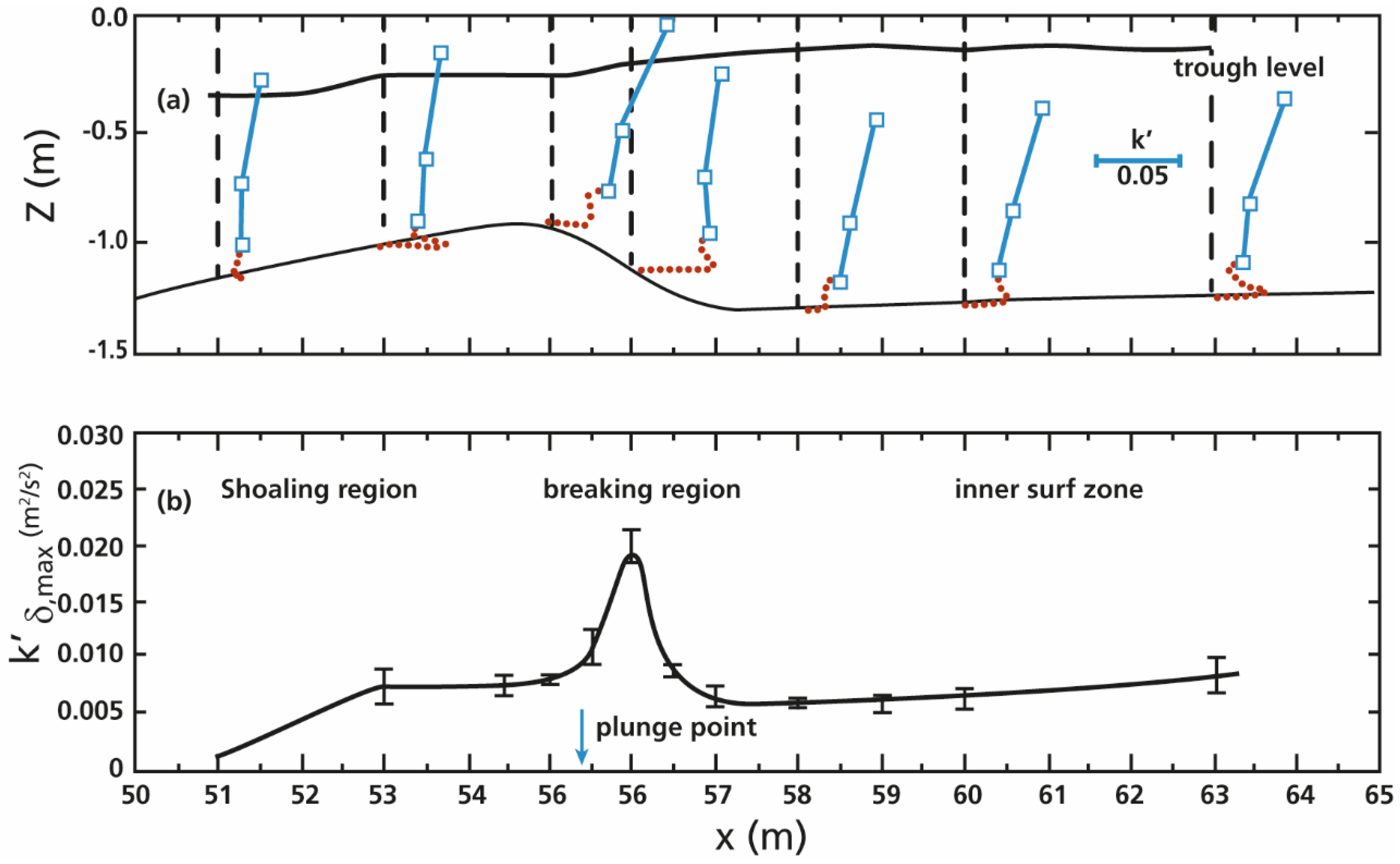
In the horizontal dimension, <k> tends to be maximum at the transition from the outer to the inner surf zone [73], i.e., at the transition from breaking waves to surf bores. This was illustrated by measurements with regular plunging breakers in a wave flume over a sandy bed [63]. Vertical profiles of <k′> were measured from trough level to the seabed with very high resolution in the boundary layer, using an Acoustic Concentration and Velocity Profiler (ACVP; Figure 9). The upper panel in the figure shows the vertical <k′> profiles which are largely consistent with the data shown in Figure 7 and Figure 8 except for the secondary maximum observed in some of the profiles very near the bed that could be resolved with the high-resolution sensor. The lower panel shows that near-bed k′_max peaked slightly landward of the main breakpoint (at x = 55–56 m) and exceeded k′_max in the shoaling and inner surf zones by a factor 3–4.

5. Sediment Mobilization and Time-Averaged Sediment Concentration

Turbulent vortices lift sediment particles off the seabed and into suspension. For non-breaking waves on a flat bed, the lift force on the particles is mainly caused by an upward-directed pressure gradient associated with the ejection of low-speed velocity streaks [11] (p. 132). When the lift force exceeds the gravity forces on the sediment particles, the grains are picked up from the bed and particle suspension is an essentially diffusive process. However, over steep vortex ripples, the suspension is fundamentally different from that associated with gradient diffusion since in this case, it is caused mainly by convective vortex shedding from the bedforms [80]. The formation of turbulent vortices over ripples was discussed briefly in Section 4 (Figure 2). Vortices form in the lee of steep ripples at orbital velocity maxima under wave crests and wave troughs, they pick up sediment from the bed and are subsequently ejected from the bed at velocity reversals [55,81,82,83,84].

Wave breaking is a particularly efficient mechanism of sediment suspension since the breaker vortices may penetrate into the wave boundary layer where sediment pick-up and hence sediment transport are significantly increased [69,79,85,86]. Overall, turbulence generated by breaking waves plays a key role for suspension in the surf zone [87]. For example, Aagaard and Hughes [28] observed that the impact of breaking waves on the seabed generated large sediment clouds, and under plunging breakers up to 85% of the suspended sediment load was associated with large breaker vortices. Clouds of sediment are lifted upward in a convective process [88], and the clouds may be advected several meters away from the breakpoint before sediment settles out of the water column [89,90]. Consequently, the suspended sediment concentration (SSC) in the water column may be several times larger under broken compared to nonbreaking waves [69].

Sumer and Fuhrman [11] explained the physical processes associated with sediment suspension under plunging breakers. Laboratory measurements of pore water pressure in a sandy bed [2] demonstrated large lift forces under plunging breakers; the lift forces created suction in the sediment bed and subsequent lifting of sediment particles. The lift was ascribed to a pressure minimum due to the breaker vortex moving in the onshore direction: At the bottom of the vortex, flow velocity is relatively small, while it is large at the top of the vortex. The pressure gradient lifts a sediment plume, such as illustrated in Figure 3 where isolated suspended sediment clouds are visible on the front face of small plunging breakers. Field observations [77,90] have shown that sediment clouds lifted by plunging breaker vortices can extend a significant distance above the bed (up to z > 50 cm) and Figure 10 shows that when plunging is violent, the clouds may occupy the entire water column.

Laboratory experiments in wave flumes have shown that inside the surf zone, mean sediment concentrations indeed scale with k rather than with u (or u²; [91,92]). Since k scales with γ (Figure 6), it might be expected that there is also a relationship between SSC and γ. This relationship is explored in Figure 11 using the same dataset and techniques as in Figure 6 and the figure shows that mean SSC was significantly larger at Durras Beach which was dominated by long-period swell waves and plunging breakers. While <k′> was largely similar for the two beaches (Figure 6a), k′_max was significantly larger at Durras Beach (Figure 6b), which again suggests that sediment suspension events are predominantly related to isolated turbulent events rather than to wave-averaged turbulence levels [93]. Unexpectedly, the effect of (mean) grain size did not appear to be critical for this dataset; at Vejers Beach, D = 0.21 mm while it was almost a factor two larger at Durras (D = 0.36 mm).

When averaged over several wave periods, the vertical distribution of suspended sediment may be described by classic concepts of gradient diffusion in the form of the time-averaged sediment convection-diffusion equation (e.g., [94]):

$$w_{c}C(z)+\overline{{\epsilon }_s\frac{dC}{dz}}=0$$

(10)

where C is the (mean) sediment concentration, z is vertical distance above the bed, and the overbar indicates wave-averaged terms. The equation states that the upward mixing of sediment, expressed through a ‘sediment diffusivity’, ε_s, is balanced by sediment settling, expressed by the sediment fall velocity, w_s. The sediment diffusivity is proportional to the vertical mixing length and a mixing velocity (${\epsilon }_s\approx l_m{w}_m$) and the property is related to eddy viscosity (ν_t; Equation (9)) which is used to model the transfer of momentum due to turbulent eddies [50]. Some doubt exists as to whether ε_s is in fact equal to ν_t; experimentally derived proportionality constants range between 0.43 [95] and 1 [96]. Assuming that the mixing velocity is expressed by $\sqrt{k}$, ε_s may be written [59]:

$${\epsilon }_s\approx l_m\sqrt{k}$$

(11)

where l_m can be estimated from measurements of the SSC-profile [97]. Using this approach, Aagaard and Jensen [77] found that for plunging breakers, ε_s was vertically invariant, while for spilling breakers and surf bores, ε_s was very small at the seabed and increased linearly upward, similar to findings by Ogston and Sternberg [95]. For nonbreaking waves over ripples, ε_s also increases upward as vortices ejected from the ripples expand and eventually dissipate [96].

As an alternative to Equation (10), vertical profiles of SSC can be predicted by modeling sediment pick-up, cw’ [50,72]. In numerical models, pick-up functions are often parameterized using proxies for c and w’, such as u and quadratic stress formulations. However, Amoudry et al. [52] found that these proxies did not provide reasonable results over rippled beds since pick-up maxima are predicted at times of maximum velocity. Instead, an approach involving shear production of k resulted in considerable improvement of their numerical model predictions. It is also doubtful whether the velocity/quadratic stress approach is appropriate for breaking wave conditions, as will be discussed in the next section.

6. Intra-Wave Properties of Turbulence and Sediment Suspension

The time-averaged bed shear stress magnitude—whether it is expressed by k, Reynolds stress, or any other relevant parameter—is crucially important to the time-averaged sediment load and therefore also to both bedload and suspended sediment transport (SST). However, in oscillatory wave-driven flows, the phase relationships between shear stress, sediment load, and u are equally important to the rates of transport. Net SST at a point (i.e., the sediment flux) under waves can be defined as:

$$\langle q_s\rangle =\langle uc\rangle =\langle u\rangle \langle c\rangle +\langle \tilde{u}\tilde{c}\rangle +\langle u^{\prime }{c}^{\prime }\rangle$$

(12)

where brackets denote time-averaged terms and tildes are non-steady (oscillatory) terms. The first term quantifies the transport associated with mean currents, the second term comprises the transport due to waves (both high-frequency sea/swell waves and infragravity waves), and the third term is turbulence transport which is usually negligible. In the following, we will consider only the high-frequency sea/swell wave component, which is critical to onshore transport of suspended sediment and depends on the co-variation (the phase coupling) between wave orbital velocity and the oscillating SSC. Numerical sediment transport models have notorious difficulties with predicting this second term. It is less than trivial to predict the wave phase where maximum shear stress (or k) production occurs—particularly since this appears to be different for different wave and seabed conditions (see earlier sections)—and even more problematic to predict the phase relationships of the sediment response. The latter involve sediment properties such as grain size and settling velocity that may result in significant lags between hydrodynamic forcing and sediment response. This section is concerned with examination of the phase-dependent intra-wave properties of turbulence and suspended sediment load.

In the relatively simple situation of non-breaking waves over flat beds, turbulent production scales with orbital velocity, and k-maxima therefore occur under wave crests and troughs, while wave nonlinearities cause asymmetries in k on wave crest and trough phases. These relationships were demonstrated, for example, in recent laboratory flume experiments [23,46] and they have also been observed in the field over low anorbital ripples [86]. Due to lags in response and lift of sediment grains, SSC is expected to lag u and k, and the lag is expected to increase vertically upward in the water column. The lag also depends on sediment grain size and wave period. Finer grains may respond more readily to forcing than coarser grains but will take longer to settle out of the water column, such that lags on increasing and decreasing SSC-phases may be different. On the other hand, long wave periods facilitate sediment mobilization and settling within the same half-wave period.

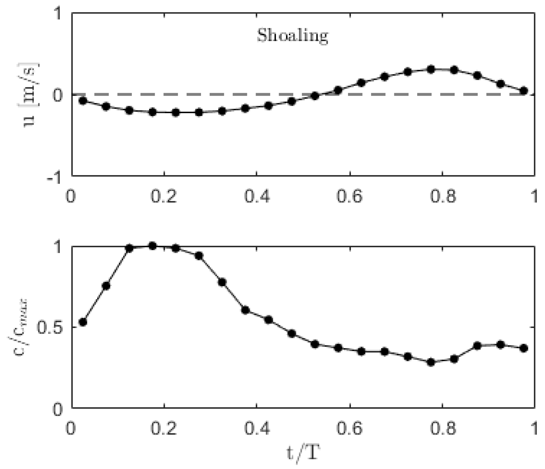
When steep wave ripples form on the seabed, bed-generated turbulence and vortex formation affect the phase relationships between SSC and wave orbital motion. For both regular [52,55] and irregular [84] laboratory waves, vortex ripples tend to produce two suspension events within the wave cycle: one at each flow reversal (Figure 2 and Figure 12). Wave skewness affects vortex strength such that positively skewed waves produce larger suspension clouds at velocity zero-downcrossing compared to clouds ejected after the trough phase (Figure 12). The regular shedding process at each flow reversal has, however, been difficult to confirm in the field, where it is in fact only rarely observed; the number of SSC-peaks within a wave cycle varies in response to both vortex strength and wave nonlinearity (e.g., [82,98]). This was exemplified by field observations under shoaling waves and low anorbital ripples [86], Figure 13. Only one SSC-peak was observed, and at z = 4 cm, the timing of the peak lagged the zero-downcrossing by 50–60° such that maximum SSC occurred on the following wave trough. For this (ensemble-averaged) irregular wave data set, there was no strong evidence for a secondary peak following the velocity zero-upcrossing.

O’Hara Murray et al. [84] suggested that vortex shedding occurs only when ripples are sufficiently steep (η/λ > 0.1), and when the ratio between orbital diameter and bedform wavelength, d_o/λ > 1.2, i.e., when the wave orbits cannot be accommodated within one ripple wavelength. A further complication in predictions of suspension events over ripples is that strong vortices favor longer life spans of the turbulent sediment-laden eddies, such that advection of suspension clouds from neighboring bed forms may occur. In this case, several suspension events may be observed within one wave cycle [98]. On the other hand, strongly skewed waves favor a single large suspension event at velocity down-crossing when orbital velocities are significantly larger beneath the wave crest compared to the wave trough [51,82]; Figure 13. All in all, prediction of turbulent production, sediment suspension and net (suspended) sediment transport rates, and directions over rippled beds is complicated due to the strong interactions between hydrodynamic processes and the still rather unpredictable geometry of the seabed.

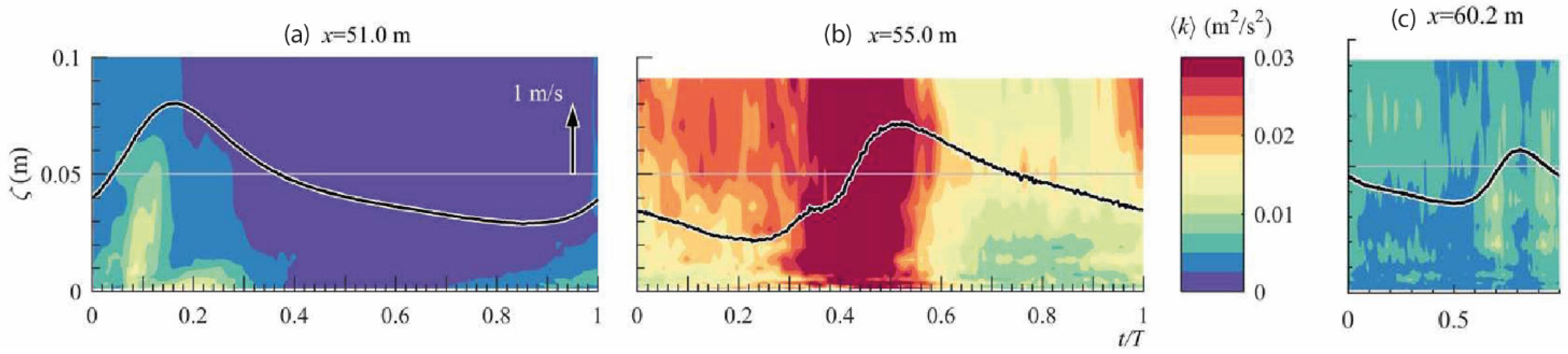
Under breaking waves, the timing of turbulence production and the travel time from the surface to the seabed become additional critical factors in the timing of k-arrival at the seabed, SSC, and consequently SST. Recent evidence points to the fact that turbulence production and propagation associated with plunging and spilling breakers, and surf bores have different characters (Section 4) and therefore affect sediment mobilization and transport differently. Van der Zanden et al. [99] presented an instructive example of the effect of different wave types on intra-wave near-bed k using LDA-measurements on a fixed bed profile without bedforms and subjected to regular waves (Figure 14). The examples show wave-cycle time series for shoaling waves, plunging breakers, and surf bores. In the shoaling wave zone, k-production originated from the planar bed on the front face of the wave and propagated upward with increasing time lag. The origin of turbulence is less clear in the plunging wave example due to the limited vertical extent of the measurement section, but k is clearly much larger and was again produced on the front face of the wave. For the sawtooth bores in the inner surf zone (x = 60.2 m), k was not well resolved over wave phase with small k-maxima on both front face and back slope of the wave but of a magnitude much smaller than for the breaking wave.

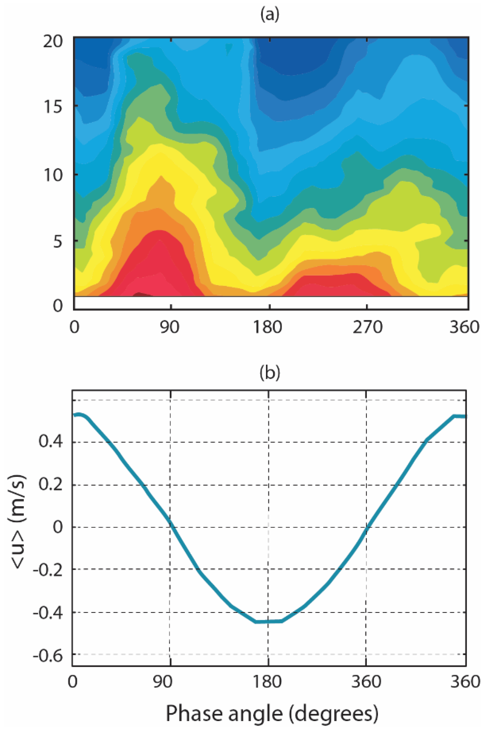
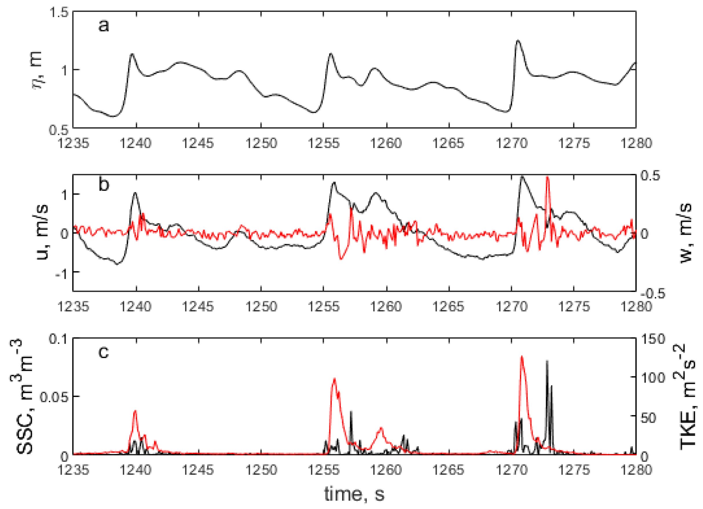
A 45-s time series of k and SSC at the plunge point of three breakers over a mobile sandy bed is shown in Figure 15. At the zero-upcrossing of each wave, w became upward-directed, followed by a succession of down/upward directed vertical velocities with a velocity amplitude of w = 0.2–0.5 m/s, associated with the rotating breaker vortex. Closer inspection shows that a phase-lead occurred between k and u; k ramped up prior to velocity maxima and was followed almost instantly by sharply defined puffs of suspended sediment. The general signatures shown in Figure 15 echo several reports [71,73,100] that point to the fact that for plunging waves, k-arrival at the seabed typically occurs under the front face, or at the crest of the waves (the relative timing probably depending on water depth (h) and the turbulent length scale (l)). For spilling breakers, however, TKE moves more slowly downward and typically arrives either on the back of the wave crest [86] (see also Figure 4), or as late as the on/offshore velocity reversal [100].

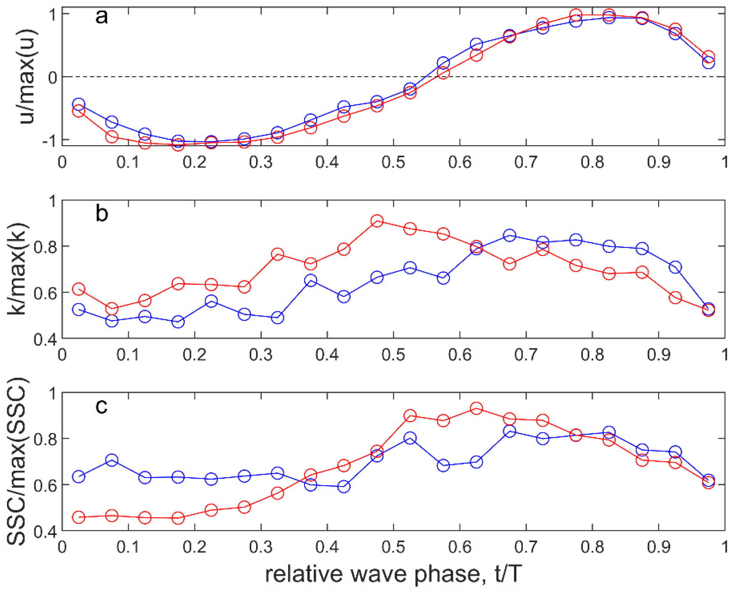
Figure 16 shows intra-wave properties of SSC using ensemble-averaged data from field measurements with both plunging and spilling breakers, for similar wave heights/water depths and mean sediment grain size (D = 0.22 mm; [72]). In these examples, ensemble-averaged k arrived at the seabed at a relative wave phase t/T ≈ 0.2 earlier for plungers than for spillers; for the former, k peaked near the zero-upcrossing, while the maximum was delayed until the wave crest phase for the latter. Sediment suspension (at z = 0.05 m) slightly lagged maximum k and was again delayed by about t/T = 0.2 for spilling waves. Based on these examples, an in-phase relationship between u and c near the bed could be a reasonable assumption for spilling waves, while for plunging waves, c clearly leads u. Closer examination of Figure 16 also reveals a different crest/trough asymmetry of both k and SSC for plunging and spilling waves; k tends to be more rapidly dissipated under plungers than under spillers. For the latter, turbulence may be carried over from one wave cycle to the next [100]. Consequently, SSC-peaks were more well-defined under plunging waves. These observations carry implications for SST under different wave types, and this will be discussed in Section 7.

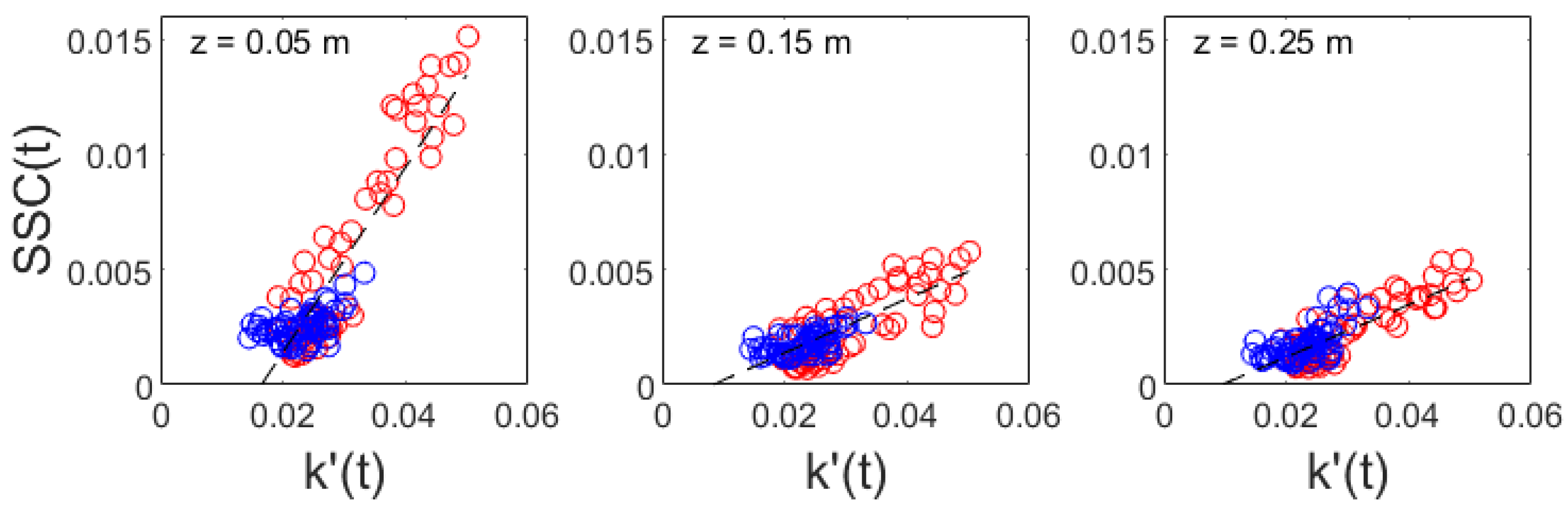
Extracting the ensemble-averaged data at each relative wave-phase bin for the six time series used in plotting Figure 16, we may examine the functional relationship between k′(t) and SSC(t) on instantaneous time scales and at different elevations above the bed (Figure 17). The plots suggest that k (or k′) may be used to predict SSC even at such instantaneous time scale; there was a statistically significant (α = 0.05) linear relationship of SSC on k′ at all elevations, but the slope of the functional relationship decreased with elevation, as would have been expected given that concentrations decrease with elevation above the bed.

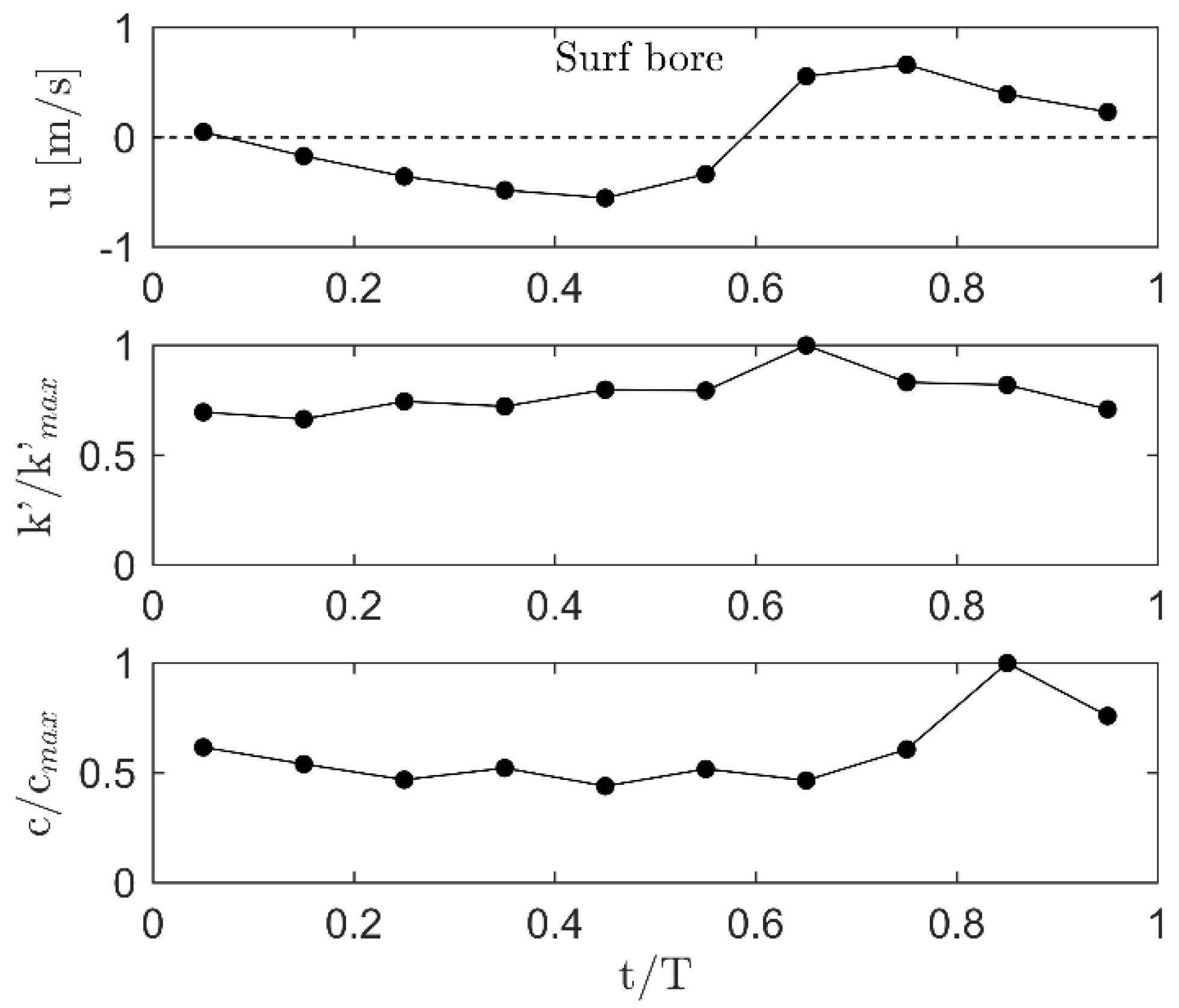
Field measurements of k and SSC on intra-wave scale under asymmetric surf bores in the inner surf zone are rare. Christensen et al. [86] observed that k-peaks occurred near the velocity zero-upcrossing, similar to plunging breakers (Figure 18), but with poorer peak definition (compare with Figure 16) and slower mixing (and/or smaller turbulent length scales), which resulted in significant lags between u and SSC. The signatures are consistent with the detailed laboratory measurements of k shown in Figure 14, which also indicated that there may be little temporal structure in the turbulent velocity signal from surf bores.

Intra-wave properties of k and SSC in the inner surf zone may be influenced by strong mean cross-and longshore currents. Wave-current interaction becomes important since strong currents that oppose the wave motion affect the wave boundary layer and increase near-bed turbulence [50], but will also distort the phase relationships between u and SSC. For example, Ruessink et al. [101] observed an increasing boundary layer thickness for situations with an opposing mean current, however, the timing of k-maxima depended on whether currents were strong or not. For purely oscillatory-flow experiments, k_max emerged under the wave crest, while in cases with a counter-current, k_max shifted backwards to the trough phase, because the offshore-directed current added to the wave-generated (bed) shear stress on the trough phase and decreased the shear stress on the crest phase. The implication is that current shear may affect the phasing of sediment suspension and further delay SSC relative to u such that maximum sediment concentrations sometimes may appear at the trough phase under surf bores [74].

The general picture that emerges from examination of available field and laboratory data on the intra-wave characteristics of SSC is that SSC-peaks are shifted forward on the wave phase with increasing turbulence levels [86], corresponding to increasing relative wave height (Figure 5). For shoaling waves over mobile (rippled) sand beds, c lags u; the ensemble-averaged examples show that c_max(t/T) occurs near the velocity zero-downcrossing (Figure 12) or even on the trough phase (Figure 13) and sometimes (but not always) with a smaller secondary peak near, or after the ensuing upcrossing, depending on wave skewness. For spilling breakers, c_max(t/T) shifts forward and is typically located on the crest/back slope of the wave, while concentration tends to lead velocity for plunging breakers; c_max(t/T) is often located on the crest/front face of the wave, as exemplified in Figure 16. For surf bores, dissipation rates are often large and even though k-maxima may occur on the front face, the slower mixing and the adverse effects of mean current shear in the inner surf zone may shift SSC-peaks backward on the wave phase. These differences carry ramifications for wave-driven transport of suspended sediment, as will be discussed next.

7. Wave-Driven Suspended Sediment Transport

Turbulence affects the rate of wave-driven suspended sediment transport because of the way it affects the magnitude of the suspended sediment load and especially the phase relationship between u and SSC. The time-averaged net flux of SST through a two-dimensional vertical section of the water column under waves and currents is defined as:

$$\langle Q_s\rangle =\frac{1}{T}{\displaystyle \underset{0}{\overset{T}{\int }}{\displaystyle \underset{0}{\overset{h}{\int }}u(z,t)c(z,t)dzdt}}$$

(13)

and <Q_s> can be further separated into mean and oscillatory terms associated with mean current and wave motions, respectively (Equation (12)). Prior to a discussion of (high-frequency sea/swell) wave-driven transport, we note that these formulae rest on the assumption that the advection speed of the sediment grains is identical to that of the surrounding fluid, u_grain = u_fluid. While that is likely to be true for very fine sediment carried as wash-load, it is more doubtful whether it also holds for sand-sized sediment. The problem was examined by Frank-Gilchrist et al. [24], who used PIV and particle tracking velocimetry (PTV) techniques to track both coarse sand grains (0.7 mm diameter) and fluid tracers. They concluded that the measured advected sediment velocities—even for sediment this coarse—were of similar magnitude and phase to the fluid velocity.

As discussed earlier, intra-wave characteristics of SSC and its magnitude is a first-order control on wave-driven SST. SSC magnitude and the phase relationship with u depend significantly on wave (breaker) type but also on sediment grain size and wave period. When suspended sediment is mobilized on the wave crest phase, coarser grain sizes and longer wave periods favour larger onshore transport rates since sediment grains may be able to settle prior to the wave trough phase. On the other hand, reduction and/or reversal of wave-driven transport may occur when strong opposing mean currents and/or smaller mixing lengths in the inner surf zone tend to shift k_max(t/T) and c_max(t/T) backwards on the wave phase. Onshore wave-driven SST is therefore often smaller under (asymmetric) surf bores in the inner surf zone than under (plunging) breakers [93]. However, despite recent progress on the qualitative understanding of these complexities, accurate scaling/parameterization of SST in the surf zone still seems some way off, partly because of measurement difficulties. Field data, in particular, notoriously contain measurement inaccuracies, for example, with respect to the elevation above the bed where variables are measured, and the risks of bubble contamination of signals from optical and acoustic sensors. Moreover, robust prediction of wave (breaker) type is still not achievable, although recent efforts [102] represent a step forward in this respect.

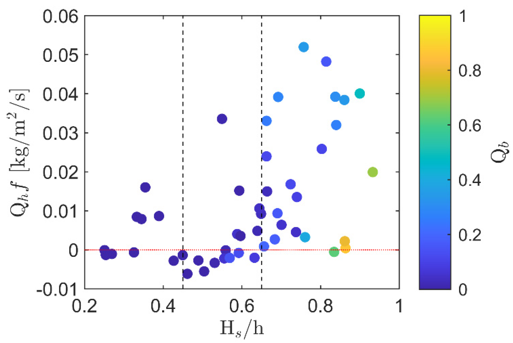
Some general characteristics have emerged on suspended sediment transport driven by incoming sea/swell waves. Brinkkemper et al. [93] measured turbulence and suspended sediment transport rates in a large-scale laboratory experiment with irregular waves, over a mobile coarse-sediment bed. They reported a clear dependency of suspended sediment transport rate and direction on the relative wave height (Figure 19). Even though there is significant scatter in the diagram, <Q_s> increased rapidly when H_s/h increased above 0.65. The diagram also illustrates the fraction of breaking waves (Q_b) which increased from the outer to the inner surf zone and when Q_b > ≈ 0.6–0.7, the high-frequency wave transport decreased dramatically.

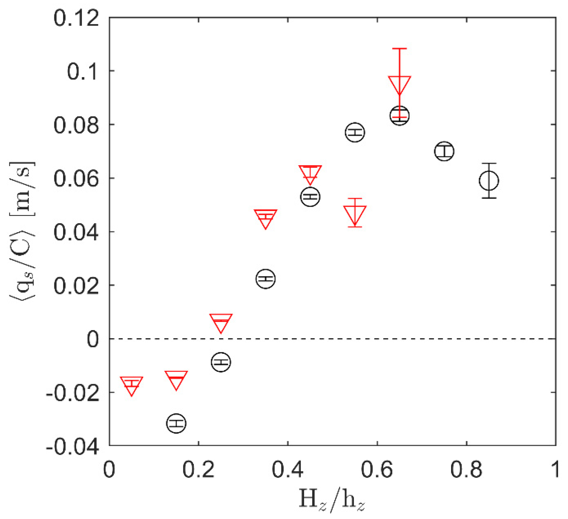
Similar results were obtained in field experiments reported by Christensen et al. [74]. In an attempt to obtain common scaling of sediment transport rates at two beaches where suspended sediment loads were very different (Figure 11), near-bed wave-driven sediment flux (q_s; Equation (12)) was normalized by the mean sediment concentration, and the ratio was termed a “flux efficiency”, F:

$$F=\frac{\langle q_s\rangle }{\langle c\rangle }$$

(14)

The dimension of F is ms⁻¹; it is a measure of transport velocity and expresses the efficiency by which the waves move a given sediment load onshore (or offshore). F was calculated for the ≈60,000 waves in the data set and averaged within γ-bins (Figure 20). Data from the two beaches follow the same trend; F was negative, signifying offshore-directed wave-driven transport under shoaling (nonbreaking) waves and became positive at the onset of wave breaking at γ ≈ 0.3. In agreement with Figure 19, the dataset with mainly plunging breakers exhibited a break-off point near γ = 0.7 where F decreased due to the strong undertow and infragravity wave activity [74] under strongly asymmetric surf bores in the inner surf zone. The dataset for mainly spilling breakers did not extend to sufficiently large γ to ascertain whether that was also the case here. Hence, given robust parameterization of <c>, it may eventually become possible to predict <qs> for different wave conditions on different beaches with different grain sizes, although much more work is required to test and refine the relationships in Figure 19 and Figure 20.

8. Summary and Future Perspectives

Beaches exist because waves restore sediment that has been lost offshore to the shoreface during storms. Wave-driven transport is of first-order importance for an onshore transport of sediment and thus beach recovery during post-storm conditions when offshore-directed mean currents weaken.

The prevailing opinion in coastal geomorphology is that beach recovery takes place during calm conditions when shoaling, non-breaking waves push sand onshore. Nevertheless, field and laboratory data overwhelmingly show that wave-driven transport in suspension is actually often directed offshore during such conditions (e.g., Figure 20), even when ripples are low and of the anorbital type (Figure 14). If significant onshore sediment transfer does occur under non-breaking calm weather conditions, it is more likely through bedload transport [103].

For sediment in suspension, onshore transport is clearly more efficient for breaking waves in the outer surf zone, particularly when waves are plunging and of long periods (corresponding to a swell wave climate). With increasing relative wave height, SSC shifts forward on the wave phase [86,93] and for plunging breakers, there is a phase lead of k and SSC relative to u; they both occur on the front face of the waves such that sediment is available for onshore transport under the entire wave crest phase.

The evidence reviewed here points to the fact that cross-shore velocity, u, or higher-order moments thereof, is a poor predictor of both suspended sediment load and wave-driven suspended sediment transport within the surf zone. Model calibration might be able to accommodate and predict the former, but not the latter, since transport depends on the phase relationship and intra-wave properties of u and SSC. Time-dependent SSC critically depends on the timing of TKE-production—which clearly depends strongly upon wave (breaker) type, and SSC is further modulated by seabed configuration and co-existing mean currents.

A robust model for wave-driven suspended sediment transport in the surf zone therefore does not yet exist. A parameterized model might be based on the observed proportionalities between normalized wave-driven SST and relative wave height (Figure 19 and Figure 20). However, these relationships clearly need further examination and testing using field (and laboratory) data from different types of beaches and with a wider range of sediment grain sizes. The critical quantity that needs to be predicted in any transport model is the SSC-magnitude, and while γ does appear to also hold some predictive capability in this respect (since it is a measure of wave energy dissipation and hence TKE-production), the scaling is different for different beaches (Figure 11). Apart from potential grain size effects, the reason is that SSC depends on the intra-wave properties of k (Figure 17) and scales with k_max rather than with $\overline{k}$.

Alternatively, more detailed process-based models of surf zone sediment transport would require resolution and prediction of k over wave phase. Encouraging progress has been made recently on simulation of time-varying turbulent properties using RANS-models [104,105] or Large Eddy Simulation [87,106] but computational demands are significant. Models for application to the surf zone would need to consider the type of wave breaking and the k/SSC lags that depend on wave (breaker) type, grain size as well as further lags associated with nonlinear interactions between waves and currents. RANS-models could be used as ‘numerical laboratories’ [105] and provided that they are sufficiently accurate, the output could be parameterized for inclusion in less complex operational models.

References

- Thorpe, S.A. The Turbulent Ocean; Cambridge University Press: Cambridge, UK, 2005; p. 439. [Google Scholar]
- Sumer, B.M.; Guner, H.A.A.; Hansen, N.M.; Fuhrman, D.R.; Fredsøe, J. Laboratory observations of flow and sediment transport induced by plunging regular waves. J. Geophys. Res. Ocean. 2013, 118, 6161–6182. [Google Scholar] [CrossRef]
- Cox, D.T.; Kobayashi, N.; Okayasu, A. Bottom shear stress in the surf zone. J. Geophys. Res. Space Phys. 1996, 101, 14337–14348. [Google Scholar] [CrossRef]
- Foster, D.L.; Beach, R.A.; Holman, R.A. Turbulence observations of the nearshore wave bottom boundary layer. J. Geophys. Res. Space Phys. 2006, 111. [Google Scholar] [CrossRef] [Green Version]
- Thornton, E.B.; Humiston, R.T.; Birkemeier, W. Bar/trough generation on a natural beach. J. Geophys. Res. Space Phys. 1996, 101, 12097–12110. [Google Scholar] [CrossRef]
- Gallagher, E.L.; Elgar, S.; Guza, R.T. Observations of sand bar evolution on a natural beach. J. Geophys. Res. Space Phys. 1998, 103, 3203–3215. [Google Scholar] [CrossRef] [Green Version]
- Mariño-Tapia, I.J.; O’Hare, T.J.; Russell, P.E.; Davidson, M.A.; Huntley, D.A. Cross-shore sediment transport on natural beaches and its relation to sandbar migration patterns: 2. Application of the field transport parameterization. J. Geophys. Res. Space Phys. 2007, 112. [Google Scholar] [CrossRef] [Green Version]
- Fuhrman, D.R.; Schløer, S.; Sterner, J. RANS-based simulation of turbulent wave boundary layer and sheet-flow sediment transport processes. Coast. Eng. 2012, 73, 151–166. [Google Scholar] [CrossRef]
- Kim, Y.; Cheng, Z.; Hsu, T.; Chauchat, J. A Numerical Study of Sheet Flow Under Monochromatic Nonbreaking Waves Using a Free Surface Resolving Eulerian Two-Phase Flow Model. J. Geophys. Res. Oceans 2018, 123, 4693–4719. [Google Scholar] [CrossRef]
- Longo, S.; Petti, M.; Losada, I.J. Turbulence in the swash and surf zones: A review. Coast. Eng. 2002, 45, 129–147. [Google Scholar] [CrossRef] [Green Version]
- Sumer, B.M.; Fuhrman, D.F. Turbulence in Coastal and Civil Engineering; Advanced Series on Ocean Engineering; World Scientific: Singapore, 2020; Volume 51, 731p. [Google Scholar]
- Aagaard, T.; Hughes, M.G. Sediment Transport. In Treatise On Coastal Geomorphology, 2nd ed.; Shroder, J.F., Ed.; Elsevier: San Diego, CA, USA, 2021; Volume 8. [Google Scholar] [CrossRef]
- Kim, S.-C.; Friedrichs, C.T.; Maa, J.P.-Y.; Wright, L.D. Estimating Bottom Stress in Tidal Boundary Layer from Acoustic Doppler Velocimeter Data. J. Hydraul. Eng. 2000, 126, 399–406. [Google Scholar] [CrossRef] [Green Version]
- Pieterse, A.; Puleo, J.A.; McKenna, T.E.; Aiken, R.A. Near-bed shear stress, turbulence production and dissipation in a shallow and narrow tidal channel. Earth Surf. Process. Landforms 2015, 40, 2059–2070. [Google Scholar] [CrossRef]
- Soulsby, R. Measurements of the Reynolds stress components close to a marine sand bank. Mar. Geol. 1981, 42, 35–47. [Google Scholar] [CrossRef]
- Pope, N.D.; Widdows, J.; Brinsley, M.D. Estimation of bed shear stress using the turbulent kinetic energy approach—A comparison of annular flume and field data. Cont. Shelf Res. 2006, 26, 959–970. [Google Scholar] [CrossRef]
- Huntley, D.A. A Modified Inertial Dissipation Method for Estimating Seabed Stresses at Low Reynolds Numbers, with Application to Wave/Current Boundary Layer Measurements. J. Phys. Oceanogr. 1988, 18, 339–346. [Google Scholar] [CrossRef] [Green Version]
- Tennekes, H.; Lumley, J.L. A First Course in Turbulence, 2nd ed.; MIT Press: Cambridge, MA, USA, 1972. [Google Scholar]
- George, R.; Flick, R.E.; Guza, R.T. Observations of turbulence in the surf zone. J. Geophys. Res. Space Phys. 1994, 99, 801–810. [Google Scholar] [CrossRef] [Green Version]
- Sleath, J.F.A. Turbulent oscillatory flow over rough beds. J. Fluid Mech. 1987, 182, 369–409. [Google Scholar] [CrossRef]
- Ting, F.C. Laboratory study of wave and turbulence velocities in a broad-banded irregular wave surf zone. Coast. Eng. 2001, 43, 183–208. [Google Scholar] [CrossRef]
- Sou, I.M.; Cowen, E.A.; Liu, P.L.-F. Evolution of the turbulence structure in the surf and swash zones. J. Fluid Mech. 2010, 644, 193–216. [Google Scholar] [CrossRef]
- O’Donoghue, T.; Davies, A.G.; Ribberink, J.S. Experimental study of the turbulent boundary layer in acceleration-skewed oscillatory flow. J. Fluid Mech. 2011, 684, 251–283. [Google Scholar] [CrossRef] [Green Version]
- Frank-Gilchrist, D.P.; Penko, A.; Calantoni, J. Investigation of Sand Ripple Dynamics with Combined Particle Image and Tracking Velocimetry. J. Atmos. Ocean. Technol. 2018, 35, 2019–2036. [Google Scholar] [CrossRef]
- Ruessink, B.G. Observations of Turbulence within a Natural Surf Zone. J. Phys. Oceanogr. 2010, 40, 2696–2712. [Google Scholar] [CrossRef] [Green Version]
- Smyth, C.; Hay, A.E. Wave Friction Factors in Nearshore Sands. J. Phys. Oceanogr. 2002, 32, 3490–3498. [Google Scholar] [CrossRef]
- Puleo, J.A.; Cristaudo, D.; Torres-Freyermuth, A.; Masselink, G.; Shi, F. The role of alongshore flows on inner surf and swash zone hydrodynamics on a dissipative beach. Cont. Shelf Res. 2020, 201, 104134. [Google Scholar] [CrossRef]
- Aagaard, T.; Hughes, M.G. Breaker vortices and sediment suspension in the surf zone. Mar. Geol. 2010, 271, 250–259. [Google Scholar] [CrossRef]
- Rodriguez, A.; Sánchez-Arcilla, A.; Redondo, J.M.; Mösso, C. Macroturbulence measurements with electromagnetic and ultrasonic sensors: A comparison under high-turbulent flows. Exp. Fluids 1999, 27, 31–42. [Google Scholar] [CrossRef]
- Cox, D.T.; Kobayashi, N. Identification of intense, intermittent coherent motions under shoaling and breaking waves. J. Geophys. Res. Space Phys. 2000, 105, 14223–14236. [Google Scholar] [CrossRef]
- Thornton, E.B. Energetics of breaking waves within the surf zone. J. Geophys. Res. Space Phys. 1979, 84, 4931–4938. [Google Scholar] [CrossRef]
- Nadaoka, K.; Hino, M.; Koyano, Y. Structure of the turbulent flow field under breaking waves in the surf zone. J. Fluid Mech. 1989, 204, 359–387. [Google Scholar] [CrossRef]
- Mocke, G.P. Structure and modeling of surf zone turbulence due to wave breaking. J. Geophys. Res. Space Phys. 2001, 106, 17039–17057. [Google Scholar] [CrossRef]
- Scott, C.P.; Cox, D.T.; Maddux, T.B.; Long, J. Large-scale laboratory observations of turbulence on a fixed barred beach. Meas. Sci. Technol. 2005, 16, 1903–1912. [Google Scholar] [CrossRef]
- Christensen, D.F.; Brinkkemper, J.; Ruessink, B.G.; Aagaard, T. Field observations of turbulence in the intertidal and shallow subtidal surf zones. Cont. Shelf Res. 2018, 170, 21–32. [Google Scholar] [CrossRef]
- Aagaard, T.; Christensen, D.F.; Hughes, M.G. Field measurements of shear stress and friction in the surf zone. Earth Surf. Process. Landforms 2020, 46, 385–398. [Google Scholar] [CrossRef]
- Bricker, J.D.; Monismith, S.G. Spectral wave-turbulence decomposition. J. Atmos. Ocean. Technol. 2007, 24, 1479–1487. [Google Scholar] [CrossRef]
- Trowbridge, J.H. On a Technique for Measurement of Turbulent Shear Stress in the Presence of Surface Waves. J. Atmos. Ocean. Technol. 1998, 15, 290–298. [Google Scholar] [CrossRef]
- Shaw, W.J.; Trowbridge, J.H. The Direct Estimation of Near-Bottom Turbulent Fluxes in the Presence of Energetic Wave Motions. J. Atmos. Ocean. Technol. 2001, 18, 1540–1557. [Google Scholar] [CrossRef]
- Feddersen, F.; Williams, A.J. Direct Estimation of the Reynolds Stress Vertical Structure in the Nearshore. J. Atmos. Ocean. Technol. 2007, 24, 102–116. [Google Scholar] [CrossRef]
- Kaimal, J.C.; Izumi, Y.; Wyngaard, J.C.; Cote, R. Spectral characteristics of surface layer turbulence. Q. J. R. Meteorological. Soc. 1972, 98, 563–589. [Google Scholar] [CrossRef]
- Brinkkemper, J.; Lanckriet, T.; Grasso, F.; Puleo, J.; Ruessink, B. Observations of turbulence within the surf and swash zone of a field-scale sandy laboratory beach. Coast. Eng. 2015, 113, 62–72. [Google Scholar] [CrossRef] [Green Version]
- Yoon, H.-D.; Cox, D.T. Cross-shore variation of intermittent sediment suspension and turbulence induced by depth-limited wave breaking. Cont. Shelf Res. 2012, 47, 93–106. [Google Scholar] [CrossRef]
- Carstensen, S.; Sumer, B.M.; Fredsøe, J. Coherent structures in wave boundary layers. Part 1. Oscillatory motion. J. Fluid Mech. 2010, 646, 169–206. [Google Scholar] [CrossRef]
- Henriquez, M.; Reniers, A.J.H.M.; Ruessink, B.G.; Stive, M.J.F. PIV measurements of the bottom boundary layer under nonlinear surface waves. Coast. Eng. 2014, 94, 33–46. [Google Scholar] [CrossRef]
- O’Donoghue, T.; Davies, A.; Bhawanin, M.; Van der A, D. Measurement and prediction of bottom boundary layer hydrodynamics under modulated oscillatory flows. Coast. Eng. 2021, 169, 103954. [Google Scholar] [CrossRef]
- Ruessink, G.; Michallet, H.; Abreu, T.; Sancho, F.; van der A, D.; Van Der Werf, J.J.; Silva, P. Observations of velocities, sand concentrations, and fluxes under velocity-asymmetric oscillatory flows. J. Geophys. Res. Space Phys. 2011, 116. [Google Scholar] [CrossRef] [Green Version]
- Gallagher, E.L.; Thornton, E.B.; Stanton, T.P. Sand bed roughness in the nearshore. J. Geophys. Res. Space Phys. 2003, 108. [Google Scholar] [CrossRef] [Green Version]
- Hay, A.E.; Mudge, T. Principal bed states during SandyDuck97: Occurrence, spectral anisotropy, and the bed state storm cycle. J. Geophys. Res. Space Phys. 2005, 110. [Google Scholar] [CrossRef] [Green Version]
- Nielsen, P. Coastal Bottom Boundary Layers and Sediment Transport. In Advanced Series on Ocean Engineering; World Scientific Publishing: Singapore, 1992; Volume 4. [Google Scholar]
- Hurther, D.; Thorne, P.D. Suspension and near-bed load sediment transport processes above a migrating, sand-rippled bed under shoaling waves. J. Geophys. Res. Space Phys. 2011, 116. [Google Scholar] [CrossRef] [Green Version]
- Amoudry, L.O.; Souza, A.J.; Thorne, P.D.; Liu, P. Parameterization of intrawave ripple-averaged sediment pickup above steep ripples. J. Geophys. Res. Oceans 2015, 121, 658–673. [Google Scholar] [CrossRef] [Green Version]
- Masselink, G.; Hughes, M.G. Introduction to Coastal Processes and Geomorphology; Hodder Arnold: London, UK, 2003; p. 354. [Google Scholar]
- Nichols, C.S.; Foster, D.L. Full-scale observations of wave-induced vortex generation over a rippled bed. J. Geophys. Res. Space Phys. 2007, 112. [Google Scholar] [CrossRef]
- Van Der Werf, J.J.; Doucette, J.S.; O‘Donoghue, T.; Ribberink, J.S. Detailed measurements of velocities and suspended sand concentrations over full-scale ripples in regular oscillatory flow. J. Geophys. Res. Space Phys. 2007, 112. [Google Scholar] [CrossRef] [Green Version]
- Van der Zanden, J.; van der A, D.A.; Caceres, I.; Larsen, B.E.; Fromant, G.; Petrotta, C.; Scandura, P.; Li, M. Spatial and temporal distributions of turbulence under bichromatic breaking waves. Coast. Eng. 2019, 146, 65–80. [Google Scholar] [CrossRef] [Green Version]
- Lin, P.; Liu, P.L.-F. Turbulence transport, vorticity dynamics and solute mixing under plunging breaking waves in surf zone. J. Geophys. Res. 1998, 103, 15677–15694. [Google Scholar] [CrossRef]
- de Serio, F.; Mossa, M. Experimental study on the hydrodynamics of regular breaking waves. Coast. Eng. 2006, 53, 99–113. [Google Scholar] [CrossRef]
- Svendsen, I.A. Analysis of surf zone turbulence. J. Geophys. Res. Space Phys. 1987, 92, 5115–5124. [Google Scholar] [CrossRef]
- Trowbridge, J.; Elgar, S. Turbulence measurements in the surf zone. J. Phys. Oceanogr. 2001, 31, 2403–2417. [Google Scholar] [CrossRef]
- Feddersen, F.; Trowbridge, J.H.; Williams, A.J. Vertical Structure of Dissipation in the Nearshore. J. Phys. Oceanogr. 2007, 37, 1764–1777. [Google Scholar] [CrossRef]
- Hsu, T.-J.; Raubenheimer, B. A numerical and field study on inner-surf and swash sediment transport. Cont. Shelf Res. 2006, 26, 589–598. [Google Scholar] [CrossRef]
- Van der Zanden, J.; van der A, D.A.; Hurther, D.; Caceres, I.; O’Donoghue, T.; Ribberink, J.S. Near-bed hydrodynamics and turbulence below a large-scale plunging breaking wave over a mobile barred bed profile. J. Geophys. Res. Ocean. 2016, 121, 6482–6506. [Google Scholar] [CrossRef] [Green Version]
- Ting, F.C.; Kirby, J.T. Dynamics of surf-zone turbulence in a spilling breaker. Coast. Eng. 1996, 27, 131–160. [Google Scholar] [CrossRef]
- Svendsen, I.A.; Madsen, P.A.; Hansen, J.B. Wave characteristics in the surf zone. In Coastal Engineering, 16th ed.; ICCE: Hamburg, Germany, 1978; pp. 529–539. [Google Scholar]
- Grasso, F.; Castelle, B.; Ruessink, G. Turbulence dissipation under breaking waves and bores in a natural surf zone. Cont. Shelf Res. 2012, 43, 133–141. [Google Scholar] [CrossRef]
- Yeh, H.H.; Mok, K.-M. On turbulence in bores. Phys. Fluids A Fluid Dyn. 1990, 2, 821–828. [Google Scholar] [CrossRef]
- Zhou, Z.; Sangermano, J.; Hsu, T.-J.; Ting, F.C.K. A numerical investigation of wave-breaking-induced turbulent coherent structure under a solitary wave. J. Geophys. Res. Oceans 2014, 119, 6952–6973. [Google Scholar] [CrossRef]
- Yu, Y.; Sternberg, R.W.; Beach, R.A. Kinematics of breaking waves and associated suspended sediment in the nearshore zone. Cont. Shelf Res. 1993, 13, 1219–1242. [Google Scholar] [CrossRef]
- Kubo, H.; Sunamura, T. Large-scale turbulence to facilitate sediment motion under spilling breakers. In Coastal Dynamics ’01; American Society of Civil Engineers: New York, NY, USA, 2001; pp. 212–221. [Google Scholar]
- de Serio, F.; Mossa, M. Experimental observations of turbulent events in the surfzone. J. Mar. Sci. Eng. 2019, 7, 332. [Google Scholar] [CrossRef] [Green Version]
- Aagaard, T.; Hughes, M.G.; Ruessink, B.G. Field observations of turbulence, sand suspension and cross-shore transport under spilling and plunging breakers. J. Geophys. Res. Earth Surf. 2018, 123, 2844–2862. [Google Scholar] [CrossRef]
- Hsu, W.; Huang, Z.; Na, B.; Chang, K.; Chuang, W.; Yang, R. Laboratory Observation of Turbulence and Wave Shear Stresses Under Large Scale Breaking Waves Over a Mild Slope. J. Geophys. Res. Oceans 2019, 124, 7486–7512. [Google Scholar] [CrossRef]
- Christensen, D.F.; Hughes, M.G.; Aagaard, T. Wave period and grain size controls on short-wave suspended sediment transport under shoaling and breaking waves. J. Geophys. Res. Earth Surf. 2019, 124, 3124–3142. [Google Scholar] [CrossRef]
- Govender, K.; Mocke, G.P.; Alport, M.J. Dissipation of isotropic turbulence and length-scale measurements through the wave roller in laboratory spilling waves. J. Geophys. Res. Space Phys. 2004, 109. [Google Scholar] [CrossRef]
- Feddersen, F. Scaling surf zone turbulence. Geophys. Res. Lett. 2012, 39. [Google Scholar] [CrossRef] [Green Version]
- Aagaard, T.; Jensen, S.G. Sediment concentration and vertical mixing under breaking waves. Mar. Geol. 2012, 336, 146–159. [Google Scholar] [CrossRef]
- Ting, F.C.; Kirby, J.T. Observation of undertow and turbulence in a laboratory surf zone. Coast. Eng. 1994, 24, 51–80. [Google Scholar] [CrossRef]
- Yoon, H.; Cox, D.T. Large-scale laboratory observations of wave breaking turbulence over an evolving beach. J. Geophys. Res. Space Phys. 2010, 115. [Google Scholar] [CrossRef]
- Davies, A.; Thorne, P. On the suspension of graded sediment by waves above ripples: Inferences of convective and diffusive processes. Cont. Shelf Res. 2015, 112, 46–67. [Google Scholar] [CrossRef] [Green Version]
- Nakato, T.; Locher, F.A.; Glover, J.R.; Kennedy, J.F. Wave entrainment of sediment from rippled beds. J. Waterw. Port Coast. Ocean. Div. 1977, 103, 83–99. [Google Scholar] [CrossRef]
- Osborne, P.D.; Greenwood, B. Sediment suspension under waves and currents: Time scales and vertical structure. Sedimentology 1993, 40, 599–622. [Google Scholar] [CrossRef]
- Mignot, E.; Hurther, D.; Chassagneux, F.-X.; Barnoud, J.-M. A field study of the ripple vortex shedding process in the shoaling zone of a macro-tidal sandy beach. J. Coast. Res. 2009, I56, 1776–1780. [Google Scholar]
- Murray, R.B.O.; Thorne, P.D.; Hodgson, D. Intrawave observations of sediment entrainment processes above sand ripples under irregular waves. J. Geophys. Res. Space Phys. 2011, 116. [Google Scholar] [CrossRef] [Green Version]
- Kana, T.W. Surf zone measurements of suspended sediment. In Coastal Engineering; ASCE: New York, NY, USA, 1978; pp. 1725–1743. [Google Scholar]
- Christensen, D.F.; Ruessink, B.G.; Brinkkemper, J.A.; Aagaard, T. Field observations of intra-wave sediment suspension in the intertidal and shallow subtidal zones. Mar. Geol. 2019, 413, 10–26. [Google Scholar] [CrossRef]
- Zhou, Z.; Hsu, T.; Cox, D.; Liu, X. Large-eddy simulation of wave-breaking induced turbulent coherent structures and suspended sediment transport on a barred beach. J. Geophys. Res. Oceans 2017, 122, 207–235. [Google Scholar] [CrossRef]
- Ting, F.C.; Beck, D.A. Observation of sediment suspension by breaking-wave-generated vortices using volumetric three-component velocimetry. Coast. Eng. 2019, 151, 97–120. [Google Scholar] [CrossRef]
- Black, K.P.; Gorman, R.M.; Symonds, G. Sediment transport near the breakpoint associated with cross-shore gradients in vertical eddy diffusivity. Coast. Eng. 1995, 26, 153–175. [Google Scholar] [CrossRef]
- Beach, R.A.; Sternberg, R.W. Suspended-sediment transport in the surf zone: Response to breaking waves. Cont. Shelf Res. 1996, 16, 1989–2003. [Google Scholar] [CrossRef]
- Yoon, H.-D.; Cox, D.; Mori, N. Parameterization of Time-Averaged Suspended Sediment Concentration in the Nearshore. Water 2015, 7, 6228–6243. [Google Scholar] [CrossRef] [Green Version]
- Van der Zanden, J.; van der A, D.A.; Hurther, D.; Caceres, I.; O’Donoghue, T.; Ribberink, J.S. Suspended sediment transport around a large-scale laboratory breaker bar. Coast. Eng. 2017, 125, 51–69. [Google Scholar] [CrossRef]
- Brinkkemper, J.A.; De Bakker, A.T.M.; Ruessink, B.G. Intrawave sand suspension in the shoaling and surf zone of a field-scale laboratory beach. J. Geophys. Res. Earth Surf. 2017, 122, 356–370. [Google Scholar] [CrossRef]
- Deigaard, R.; Fredsøe, J.; Hedegaard, I.B. Suspended Sediment in the Surf Zone. J. Waterw. Port. Coastal Ocean Eng. 1986, 112, 115–128. [Google Scholar] [CrossRef]
- Ogston, A.; Sternberg, R. Effect of wave breaking on sediment eddy diffusivity, suspended-sediment and longshore sediment flux profiles in the surf zone. Cont. Shelf Res. 2002, 22, 633–655. [Google Scholar] [CrossRef]
- Thorne, P.D.; Davies, A.G.; Bell, P.S. Observations and analysis of sediment diffusivity profiles over sandy rippled beds under waves. J. Geophys. Res. Space Phys. 2009, 114. [Google Scholar] [CrossRef] [Green Version]
- Nielsen, P. Suspended sediment concentrations under waves. Coast. Eng. 1986, 10, 23–31. [Google Scholar] [CrossRef]
- Villard, P.V.; Osborne, P.D. Visualization of wave-induced suspension patterns over two-dimensional bedforms. Sedimentology 2002, 49, 363–378. [Google Scholar] [CrossRef]
- van der Zanden, J.; van der A, D.A.; Caceres, I.; Hurther, D.; McLelland, S.J.; Ribberink, J.S.; O’Donoghue, T. Near-bed turbulent kinetic energy budget under a large-scale plunging breaking wave over a fixed bar. J. Geophys. Res. Ocean. 2018, 123, 1429–1456. [Google Scholar] [CrossRef]
- Ting, F.C. Laboratory measurements of large-scale near-bed turbulent flow structures under plunging regular waves. Coast. Eng. 2013, 77, 120–139. [Google Scholar] [CrossRef]
- Ruessink, B.; Ramaekers, G.; van Rijn, L. On the parameterization of the free-stream non-linear wave orbital motion in nearshore morphodynamic models. Coast. Eng. 2012, 65, 56–63. [Google Scholar] [CrossRef]
- Carini, R.J.; Chickadel, C.C.; Jessup, A.T. Surf Zone Waves at the Onset of Breaking: 2. Predicting Breaking and Breaker Type. J. Geophys. Res. Oceans 2021, 126. [Google Scholar] [CrossRef]
- Mieras, R.S.; Puleo, J.A.; Anderson, D.; Hsu, T.; Cox, D.T.; Calantoni, J. Relative Contributions of Bed Load and Suspended Load to Sediment Transport Under Skewed-Asymmetric Waves on a Sandbar Crest. J. Geophys. Res. Oceans 2019, 124, 1294–1321. [Google Scholar] [CrossRef]
- Larsen, B.E.; Fuhrman, D.R. On the over-production of turbulence beneath surface waves in Reynolds-averaged Navier–Stokes models. J. Fluid Mech. 2018, 853, 419–460. [Google Scholar] [CrossRef] [Green Version]
- Larsen, B.E.; van der A, D.A.; van der Zanden, J.; Ruessink, G.; Fuhrman, D.R. Stabilized RANS simulation of surf zone kinematics and boundary layer processes beneath large-scale plunging waves over a breaker bar. Ocean. Model. 2020, 155, 101705. [Google Scholar] [CrossRef]
- Christensen, E.D. Large eddy simulation of spilling and plunging breakers. Coast. Eng. 2006, 53, 463–485. [Google Scholar] [CrossRef]
Figure 1.
Phase and coherence plots from u-w co-spectral analysis of field data. The dashed lines in the phase plot indicate phases of ±π/2 and in the coherence plot, it indicates the level of statistically significant coherence. The red dashed lines indicate the selected cut-off frequency between wave motions and turbulence (in this case f = 0.62 Hz).
Figure 2.
Idealized sketch of sediment clouds produced by turbulent vortex generation over steep wave ripples in an oscillatory flow. Reprinted from Masselink and Hughes [53] with permission from Informa UK Ltd through PLSclear.
Figure 3.
Photos of a plunging breaker (left) and a spilling breaker (right). The arrows in the left image point toward isolated sediment clouds lifted by the plunging breaker.
Figure 4.
Two-dimensional image from a large-eddy-simulation of spanwise-averaged turbulent intensity under a spilling breaker. Note the considerable distance between the production of turbulence under the wave crest and its intersection with the seabed under the back slope of the wave. Adapted from Zhou et al. [68] with permission from John Wiley and Sons.
Figure 5.
Record-averaged <k′> at two beaches dominated by swell waves with typically plunging breakers (dots) and wind waves breaking predominantly as spillers breakers (crosses). Turbulence was measured at nominal elevations of z = 50 cm (black symbols), z = 20 cm (blue symbols), and z = 5 cm (light blue). Modified from Christensen et al. [74].
Figure 6.
Near-bed (z = 0.05–0.10 m) wave-cycle and bin-averaged <k′> (a) and k′max (b) plotted against relative zero-crossing wave height (Hz/hz). Red symbols are for Vejers beach with mainly spilling breakers while black symbols represent the swell-dominated beach at Durras with mainly plunging breakers. The vertical bars show the standard error on the means within each γ-bin. From Christensen et al. [74].
Figure 7.
First-EOF-derived structure of turbulent dissipation rate (ε), plotted against elevation above the bed for different wave conditions: breaking waves (blue symbols), surf bores (green symbols), and transitional conditions (red symbols). Horizontal and vertical brackets represent the 99% confidence intervals. Reproduced from Grasso et al. [66] with permission from Elsevier.
Figure 8.
Vertical structure of <k′> for non-breaking waves (γs = 0.1–0.3, panel (a)), weakly breaking waves (γs = 0.3–0.5, panel (b)) and strongly breaking waves (γs > 0.5, panel (c)). z is elevation above the seabed. Black symbols are from Durras Beach, NSW, Australia and red symbols are from Vejers Beach, Denmark. From Christensen et al. [74].
Figure 9.
(a). Cross-shore evolution of the vertical <k′>-structure under monochromatic waves measured by ADVs (blue line and squares) and ACVP (red dots) in a laboratory facility. The cross-shore profile is shown for reference. (b). Maximum <k′> measured within the wave boundary layer. Modified from van der Zanden et al. [63].
Figure 10.
Plunging breaker at the beach step on the reflective beach at Anloga, Ghana. Note the reddish-brown color of the water in the overturning wave, which is caused by suspended sediment particles that have been picked up by the breaker.
Figure 11.
Near-bed suspended sediment concentration plotted against relative zero-crossing wave height. Black circles are data from Durras Beach (swell-wave dominated with mainly plunging breakers) and red triangles are data from Vejers beach (wind-wave dominated beach with mainly spilling breakers). The vertical bars show the standard error on the mean value within each γ-bin. From Christensen et al. [74].
Figure 12.
(a) Intra-wave variation in SSC with elevation above the bed (measured in cm), plotted against wave phase for a laboratory experiment over a mobile rippled bed. Warm colors indicate large SSC. Panel (b) shows ensemble-averaged orbital velocity. Positive velocities are onshore directed. Adapted from O’Hara Murray et al. [84] with permission from John Wiley and Sons.
Figure 13.
Ensemble-averaged cross-shore velocity (upper panel) and sediment concentration at z = 4 cm (lower panel) under skewed, shoaling waves at Vejers Beach, Denmark. The relative wave height, γs = 0.30, the ripple height η = 1.18 cm, and ripple steepness η/λ = 0.15. Velocity skewness SKu = 0.334. Reproduced from Christensen et al. [86].
Figure 14.
Time series of depth-varying phase-averaged turbulent kinetic energy (<k>) in the lower 10 cm of the water column for (a) shoaling waves (x = 51.0 m), (b) plunging breakers (x = 55.0 m), and (c) surf bores (x = 60.2 m). x indicates the along-flume distance from the wave generator and the magnitude of <k> is indicated by the right-hand scale. The free-stream velocity is shown in each panel by the black line. Modified from van der Zanden et al. [99].
Figure 15.
Time series of surface elevation (a), cross-shore (u, black line) and vertical (w, red line) velocity (b), and (panel (c)) turbulent kinetic energy (TKE, black line) and suspended sediment concentration (SSC) at z = 3.5 cm (red line) for three plunging breakers at Durras Beach, NSW.
Figure 16.
Ensemble-averaged measurements of normalized (a) cross-shore velocity, (b) turbulent kinetic energy, and (c) SSC for predominantly spilling (blue lines) and plunging (red lines) breakers at z = 0.05 m. Data were combined from six time series, comprising three series with mainly plunging breakers and three series with spilling breakers. Reproduced from Aagaard et al. [72].
Figure 17.
Ensemble-averaged sediment concentrations at (nominally) z = 0.05, 0.15 and 0.25 m, as a function of ensemble-averaged Froude-scaled turbulent kinetic energy. Red color: Plunging breakers, blue color: spilling breakers. The relationships have coefficients of determination, r2 = 0.81, 0.63, 0.67, respectively. Reproduced from Aagaard et al. [72].
Figure 18.
Ensemble-averaged cross-shore velocity (upper panel) and normalized k (middle panel) and suspended sediment concentration at z = 5 cm (lower panel) under asymmetric surf bores in the intertidal zone at Vejers Beach, Denmark. Bedforms were absent, the relative wave height, γs = 0.64, and velocity asymmetry ASu = 1.95. From Christensen et al. [86].
Figure 19.
Wave-driven high-frequency suspended sediment transport, Qhf (cumulated over three sensors in the vertical) plotted against relative wave height, Hs/h. The colors indicate the fraction of broken waves in the time series (Qb). Positive Qhf is onshore directed. Reproduced from Brinkkemper et al. [93].
Figure 20.
Near-bed (z < 10 cm) flux efficiency (F = <qs>/<c>) plotted against relative zero-crossing wave height for two beaches dominated by plunging (black circles) and spilling (red triangles) breakers. Positive F is onshore directed. The vertical bars denote the standard error on the mean values. Modified from Christensen et al. [74].
Publisher’s Note: MDPI stays neutral with regard to jurisdictional claims in published maps and institutional affiliations. |
© 2021 by the authors. Licensee MDPI, Basel, Switzerland. This article is an open access article distributed under the terms and conditions of the Creative Commons Attribution (CC BY) license (https://creativecommons.org/licenses/by/4.0/).
Share and Cite
MDPI and ACS Style
Aagaard, T.; Brinkkemper, J.; Christensen, D.F.; Hughes, M.G.; Ruessink, G. Surf Zone Turbulence and Suspended Sediment Dynamics—A Review. J. Mar. Sci. Eng. 2021, 9, 1300. https://doi.org/10.3390/jmse9111300
AMA Style
Aagaard T, Brinkkemper J, Christensen DF, Hughes MG, Ruessink G. Surf Zone Turbulence and Suspended Sediment Dynamics—A Review. Journal of Marine Science and Engineering. 2021; 9(11):1300. https://doi.org/10.3390/jmse9111300
Chicago/Turabian StyleAagaard, Troels, Joost Brinkkemper, Drude F. Christensen, Michael G. Hughes, and Gerben Ruessink. 2021. "Surf Zone Turbulence and Suspended Sediment Dynamics—A Review" Journal of Marine Science and Engineering 9, no. 11: 1300. https://doi.org/10.3390/jmse9111300
Note that from the first issue of 2016, this journal uses article numbers instead of page numbers. See further details here.