Author Contributions
Conceptualization, M.V., D.V., and R.T.; methodology, M.V., D.V., B.P. and A.F.; software, D.V., B.P. and A.F.; M.V., D.V. and A.F.; formal analysis, M.V., D.V., B.P. and R.T.; investigation, D.V. and A.F.; resources, M.V., D.V. and A.F.; data curation, A.F.; writing—original draft preparation, M.V., D.V. and A.F.; writing—review and editing, M.V., D.V., B.P., R.T. and A.F.; visualization, A.F.; supervision, M.V., D.V. and R.T.; project administration, M.V. and D.V. All authors have read and agreed to the published version of the manuscript.
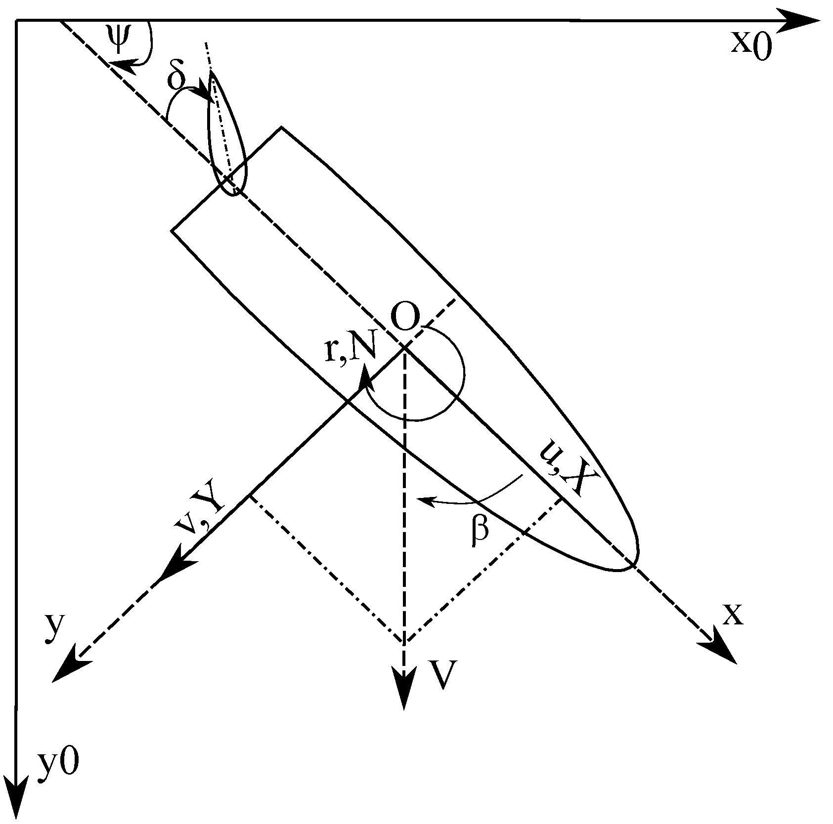
Figure 1.
Manoeuvrability sign convention.
Figure 1.
Manoeuvrability sign convention.
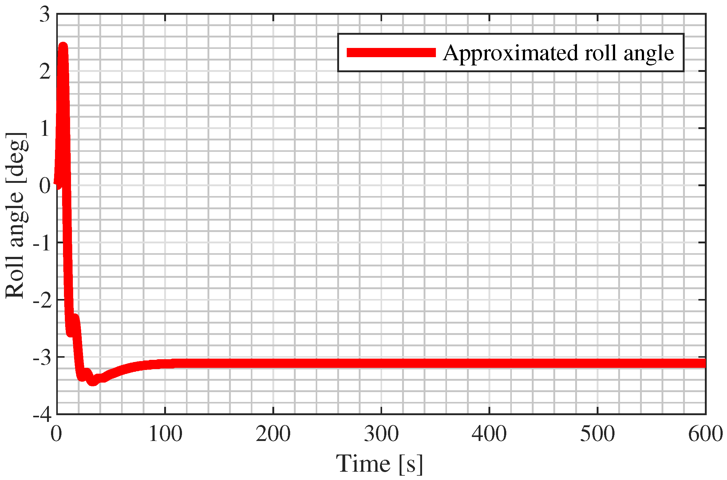
Figure 2.
Roll angle in turning circle 35 [deg] manoeuvre.
Figure 2.
Roll angle in turning circle 35 [deg] manoeuvre.
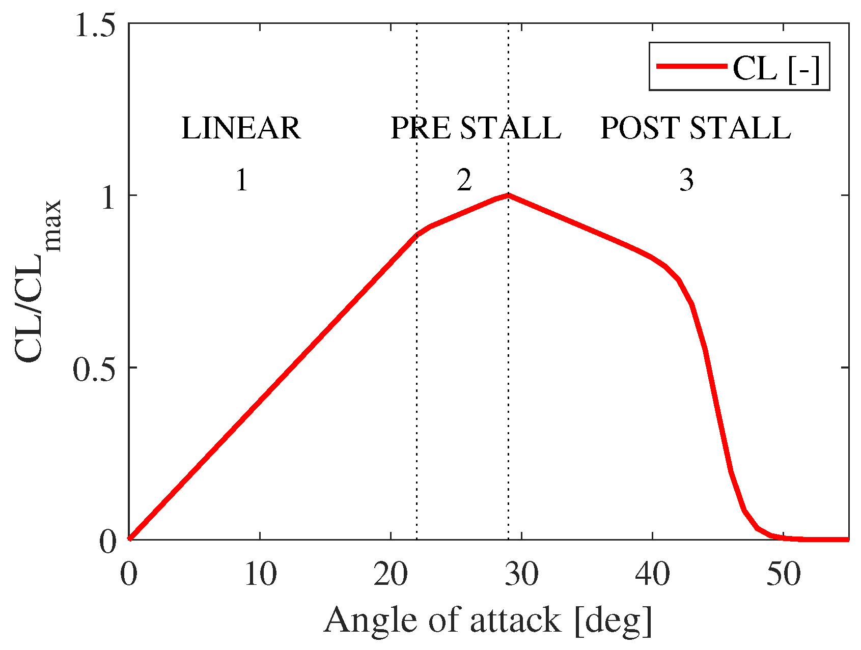
Figure 3.
Lift coefficient of the rudder implemented in the simulator.
Figure 3.
Lift coefficient of the rudder implemented in the simulator.
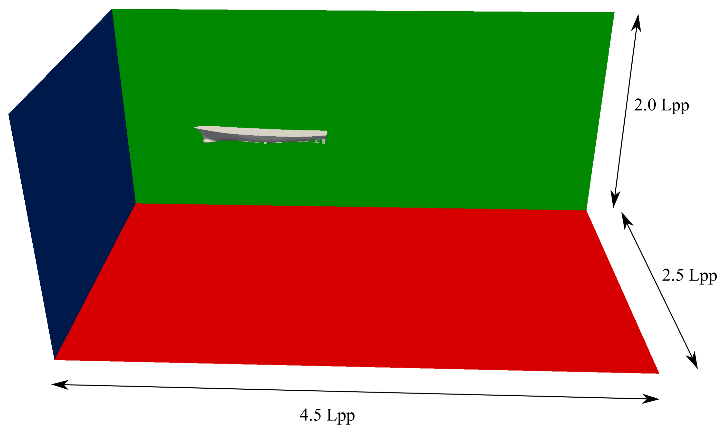
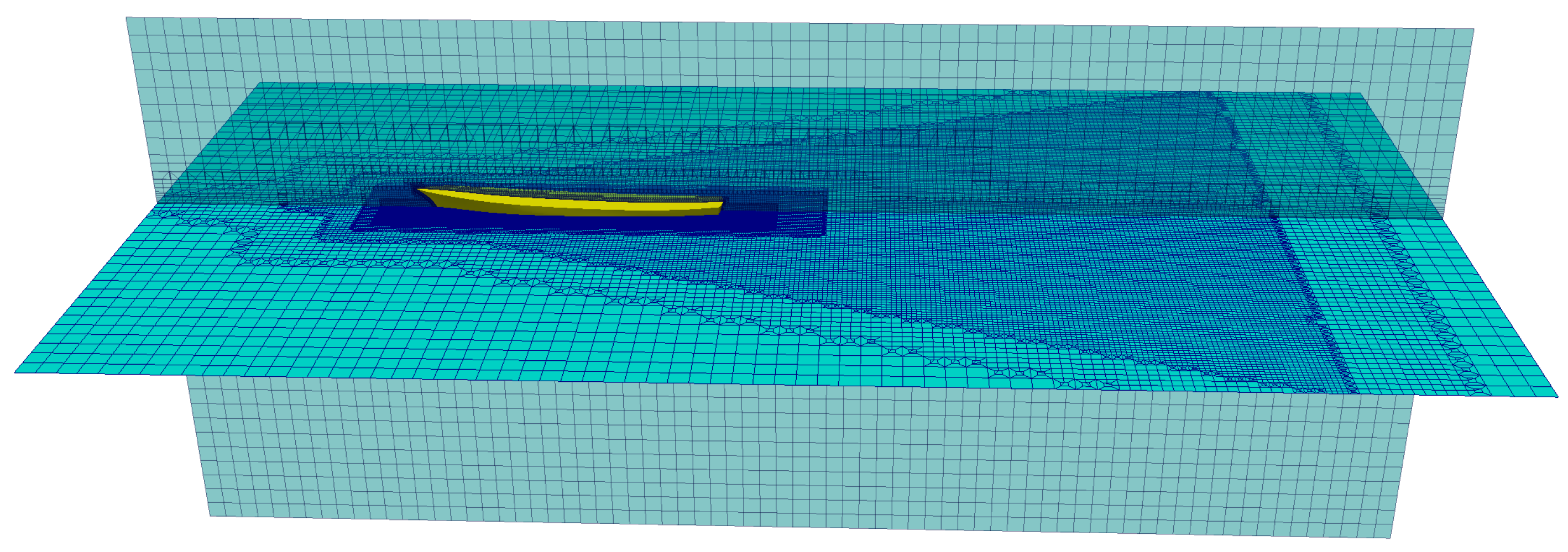
Figure 4.
Computational domain.
Figure 4.
Computational domain.
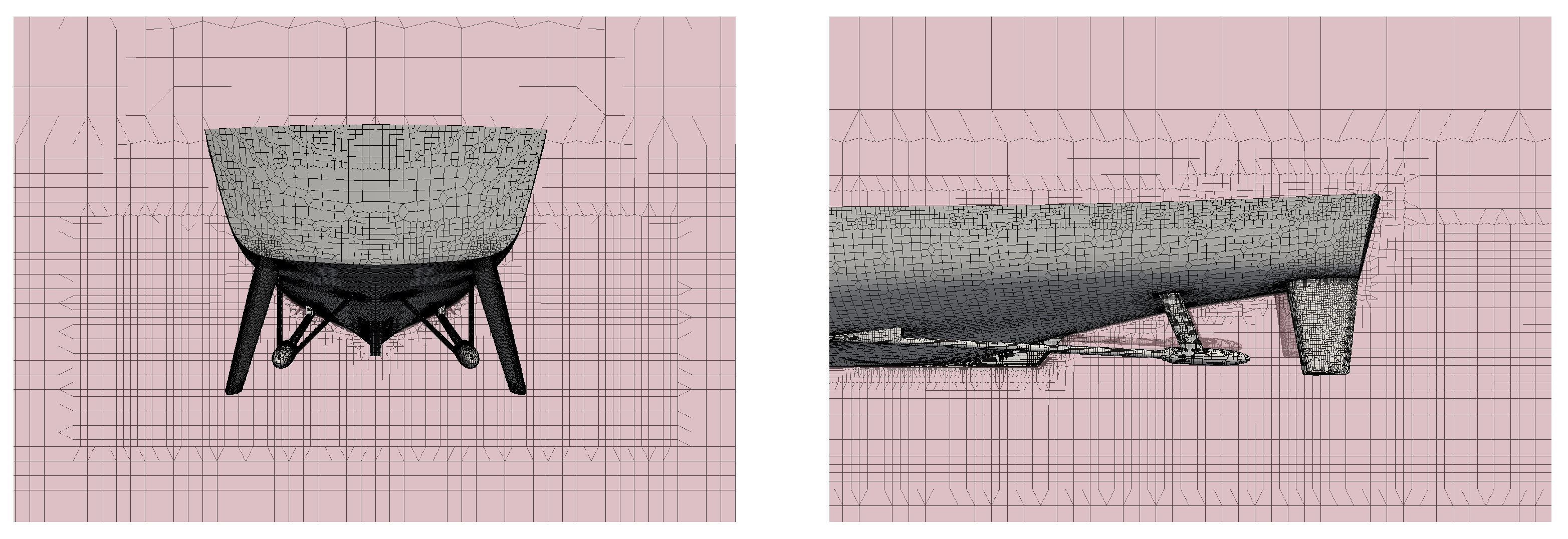
Figure 5.
Mesh in the pure drift test.
Figure 5.
Mesh in the pure drift test.
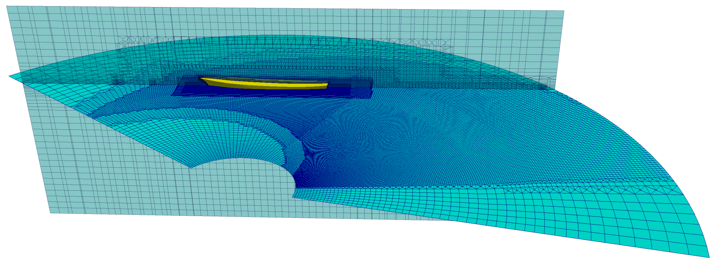
Figure 6.
Mesh in the rotation test.
Figure 6.
Mesh in the rotation test.
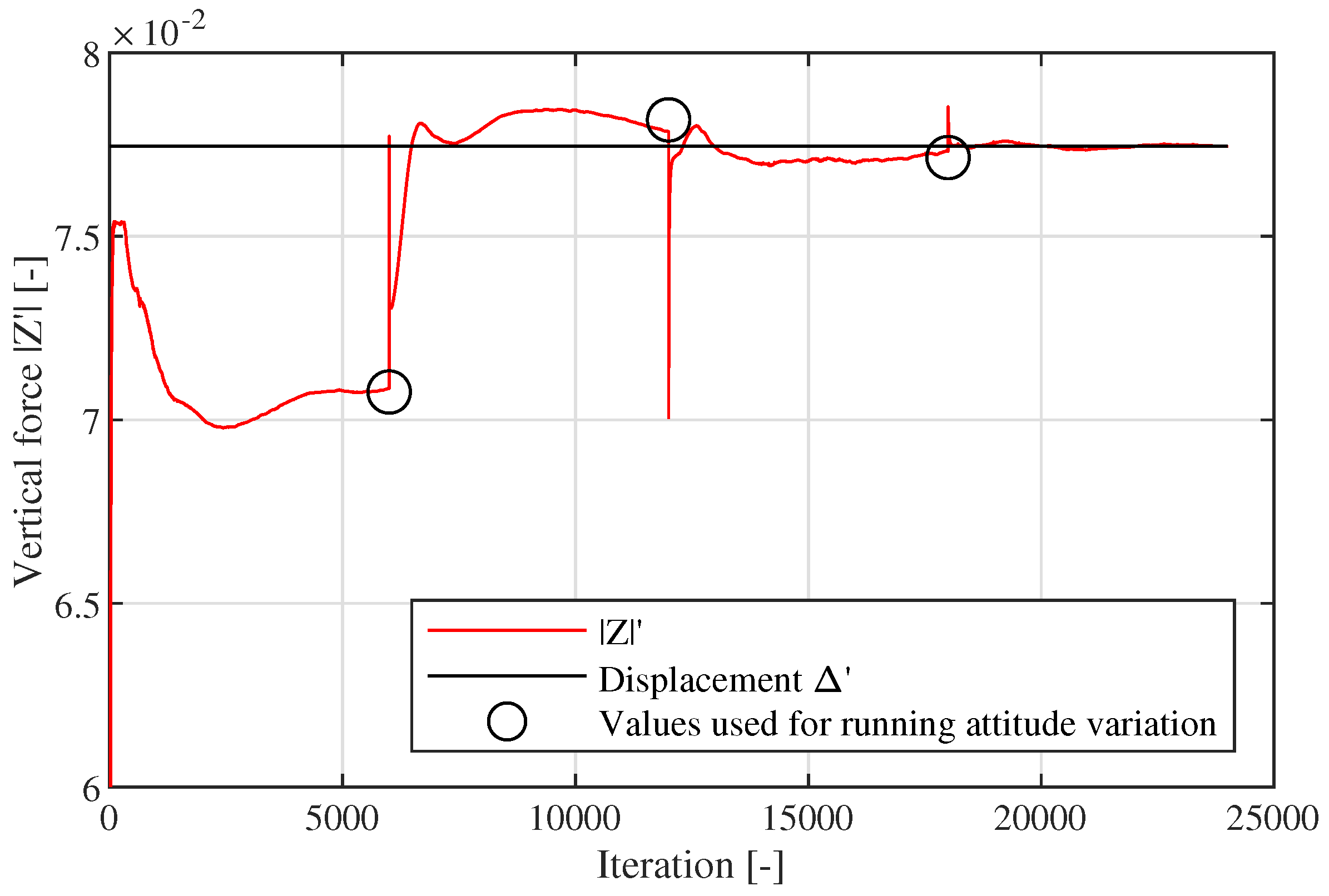
Figure 7.
Iterative process of the vertical force balance.
Figure 7.
Iterative process of the vertical force balance.
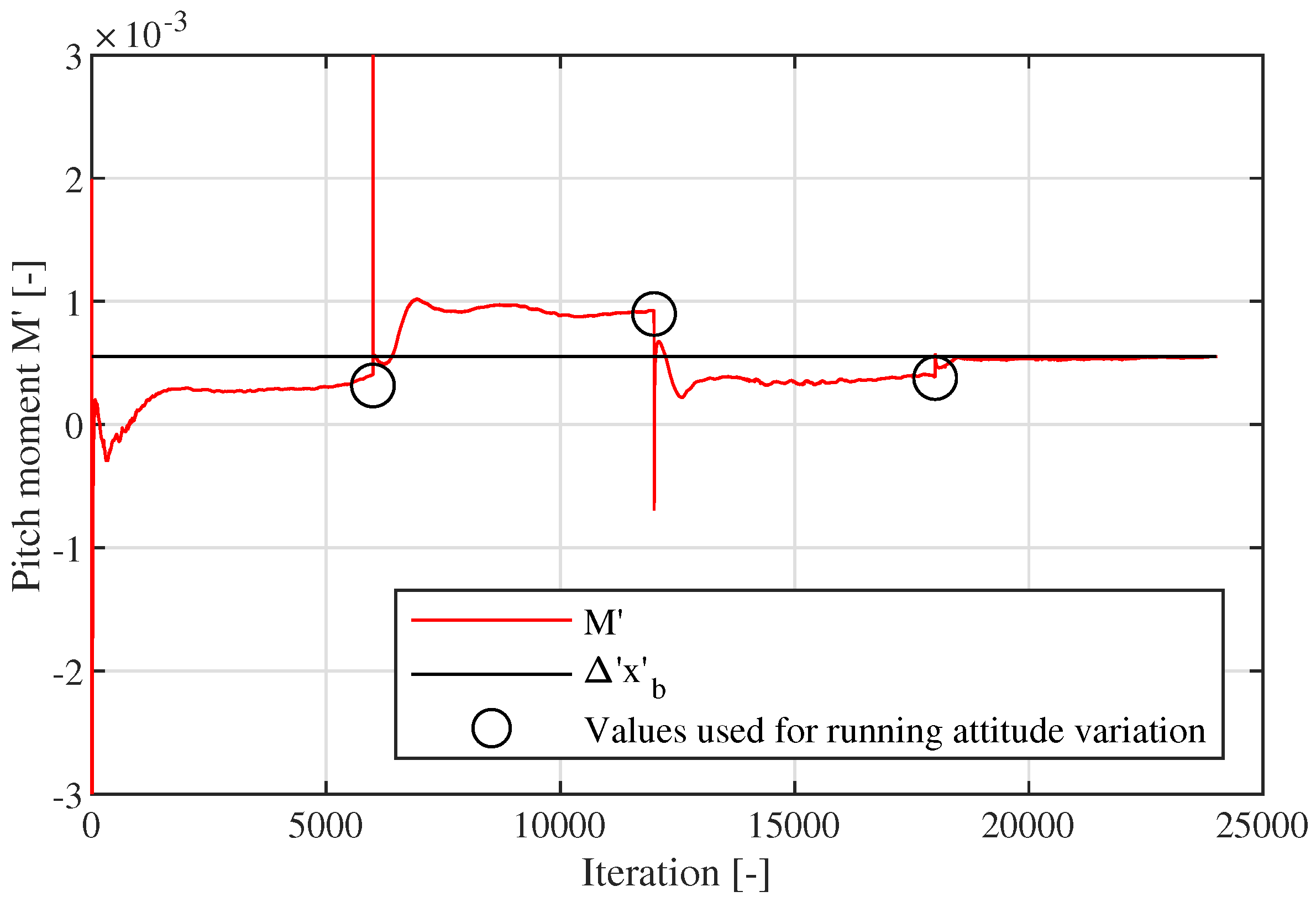
Figure 8.
Iterative process of the pitch moment balance.
Figure 8.
Iterative process of the pitch moment balance.
Figure 9.
Refinement of the surface mesh on the aft of the ship.
Figure 9.
Refinement of the surface mesh on the aft of the ship.
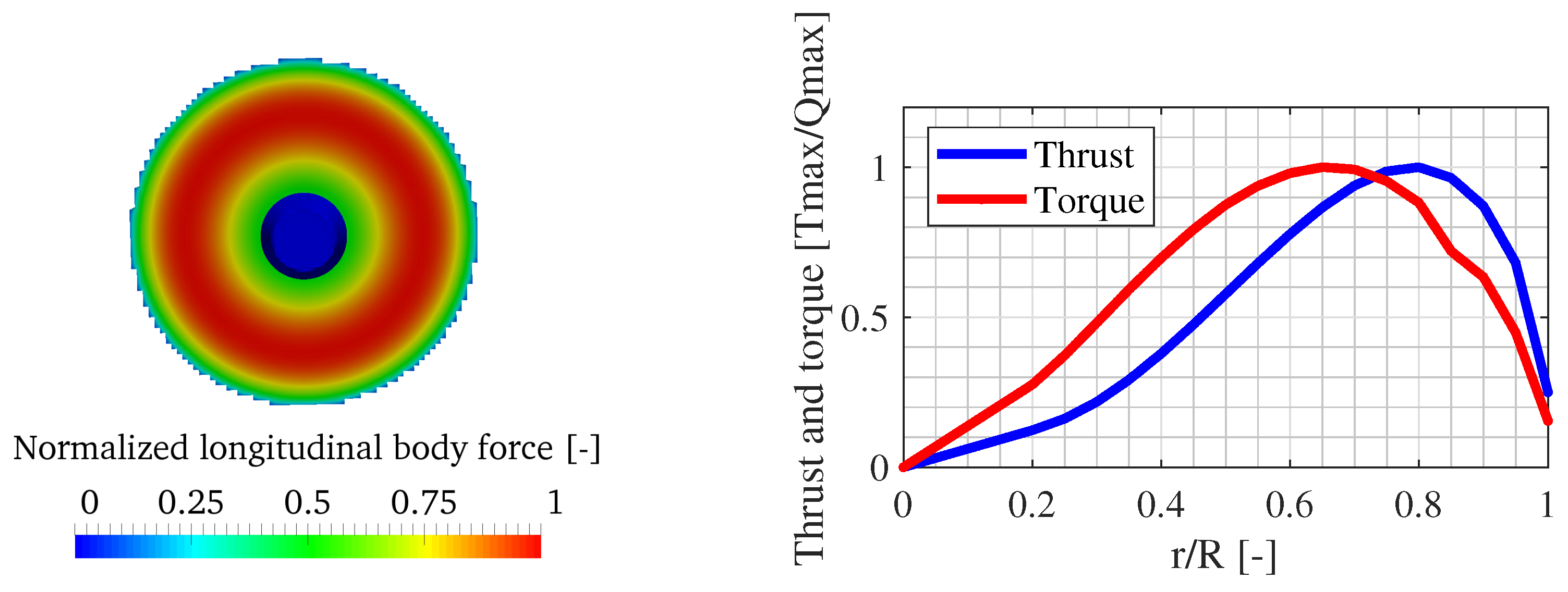
Figure 10.
The actuator disk body force radial distribution.
Figure 10.
The actuator disk body force radial distribution.
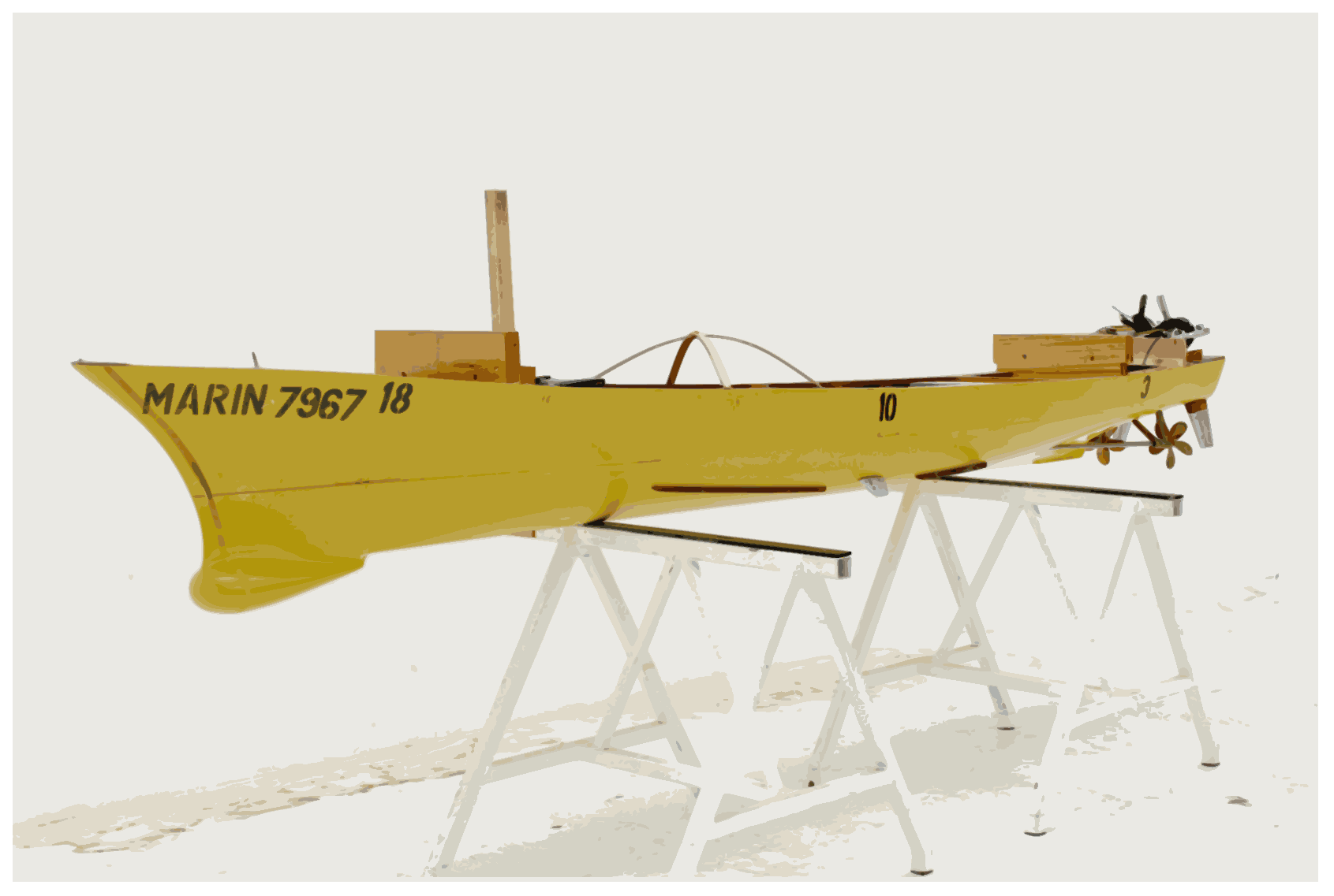
Figure 11.
The 5415 M model in MARIN facilities.
Figure 11.
The 5415 M model in MARIN facilities.
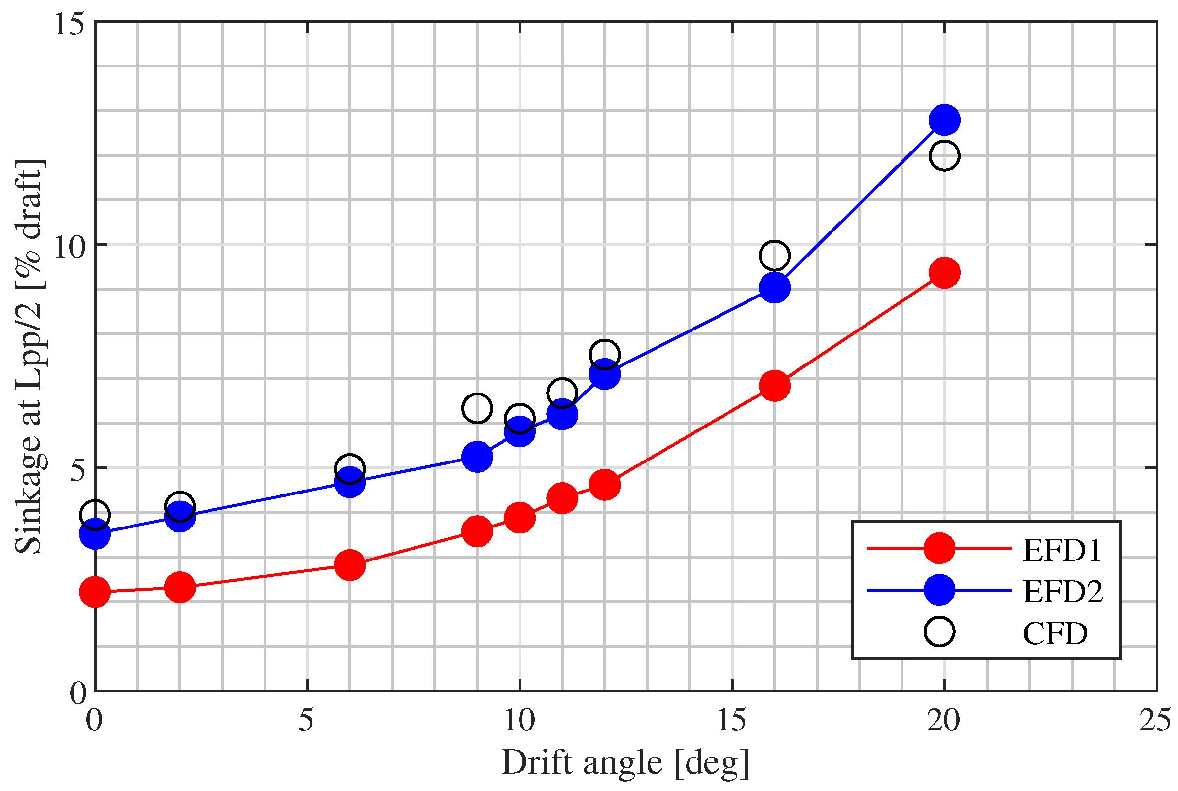
Figure 12.
Experimental vs. numerical sinkage at midship.
Figure 12.
Experimental vs. numerical sinkage at midship.
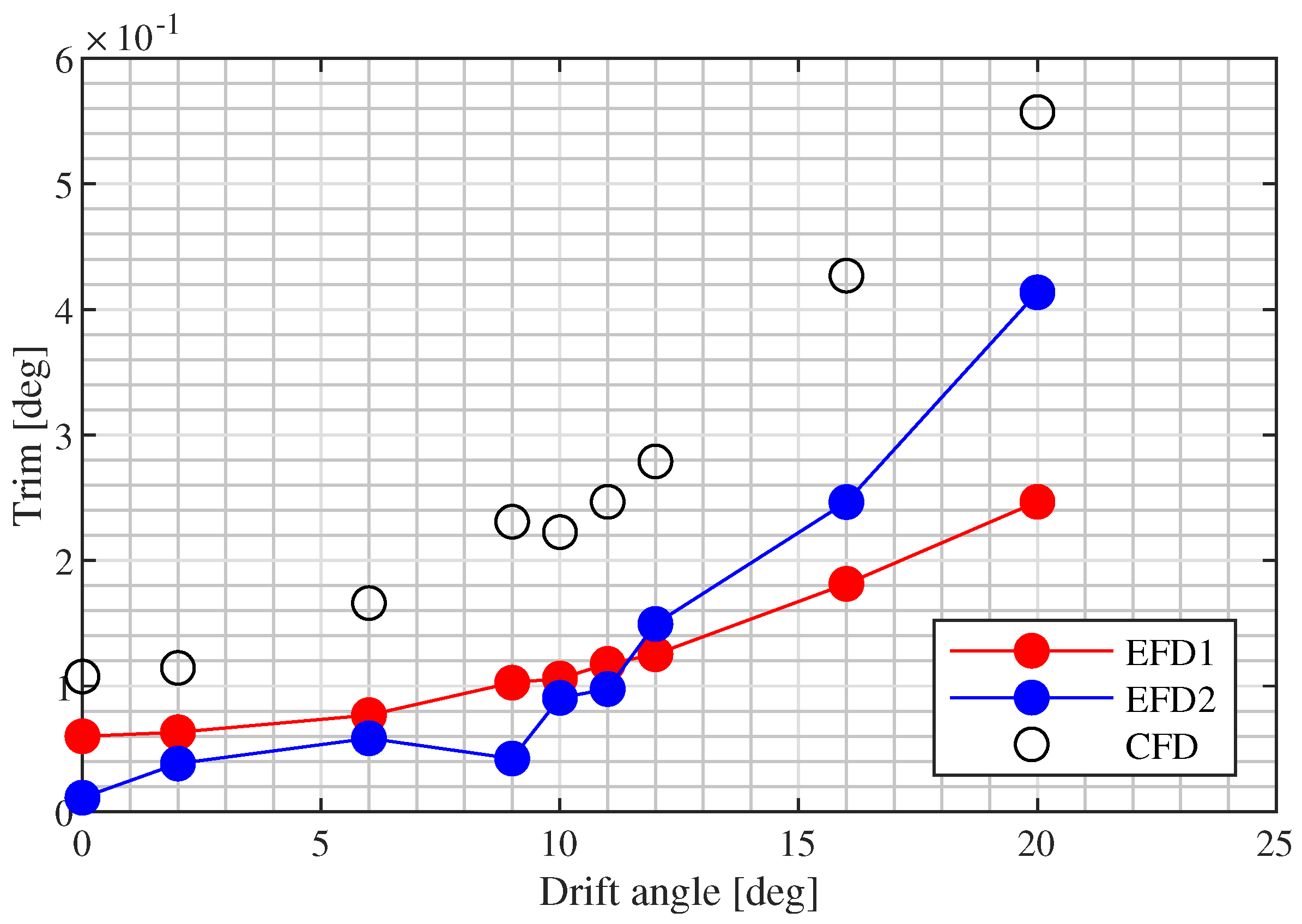
Figure 13.
Experimental vs. numerical trim.
Figure 13.
Experimental vs. numerical trim.
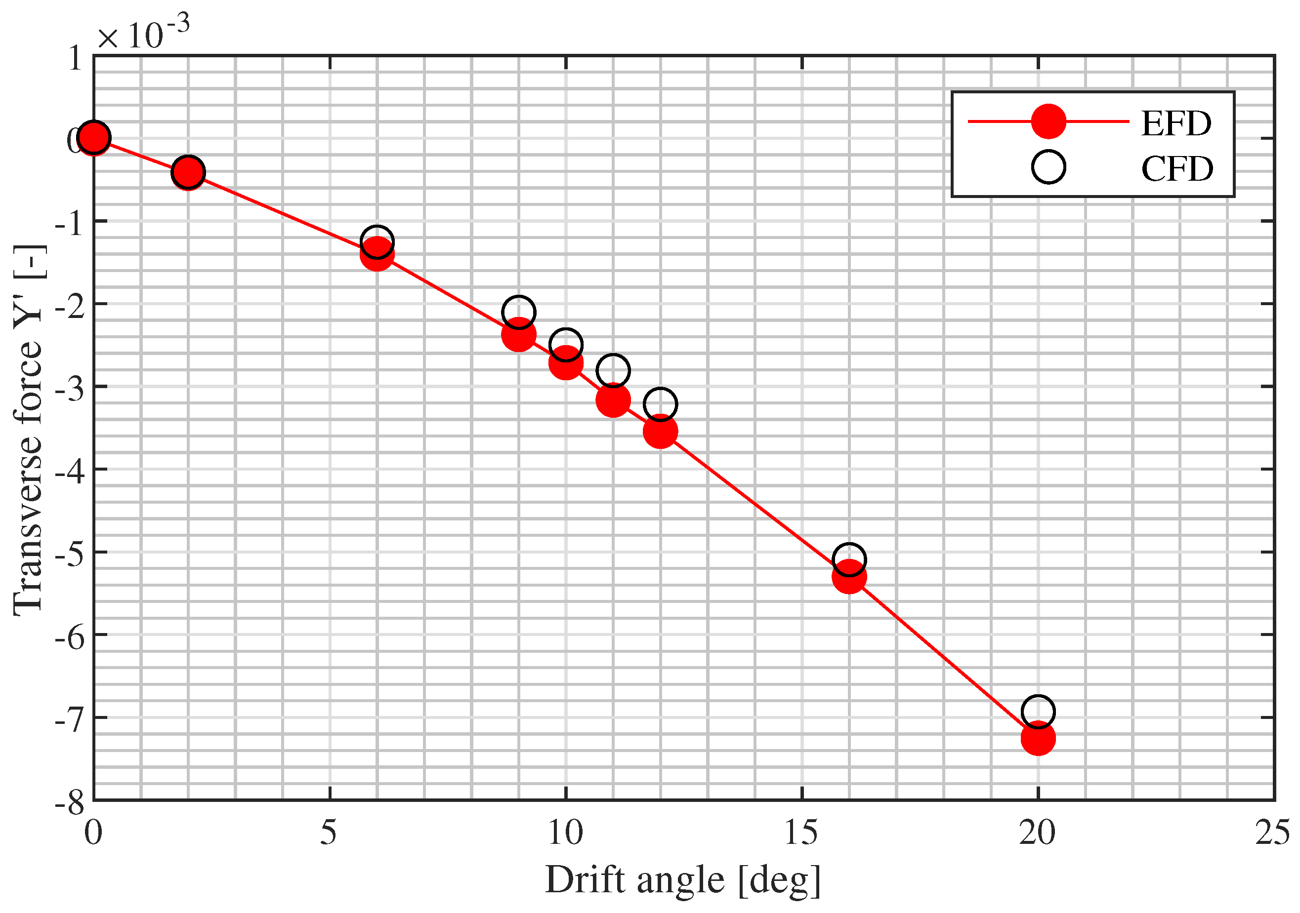
Figure 14.
Transverse force Y’ in the static drift tests-bare hull configuration.
Figure 14.
Transverse force Y’ in the static drift tests-bare hull configuration.
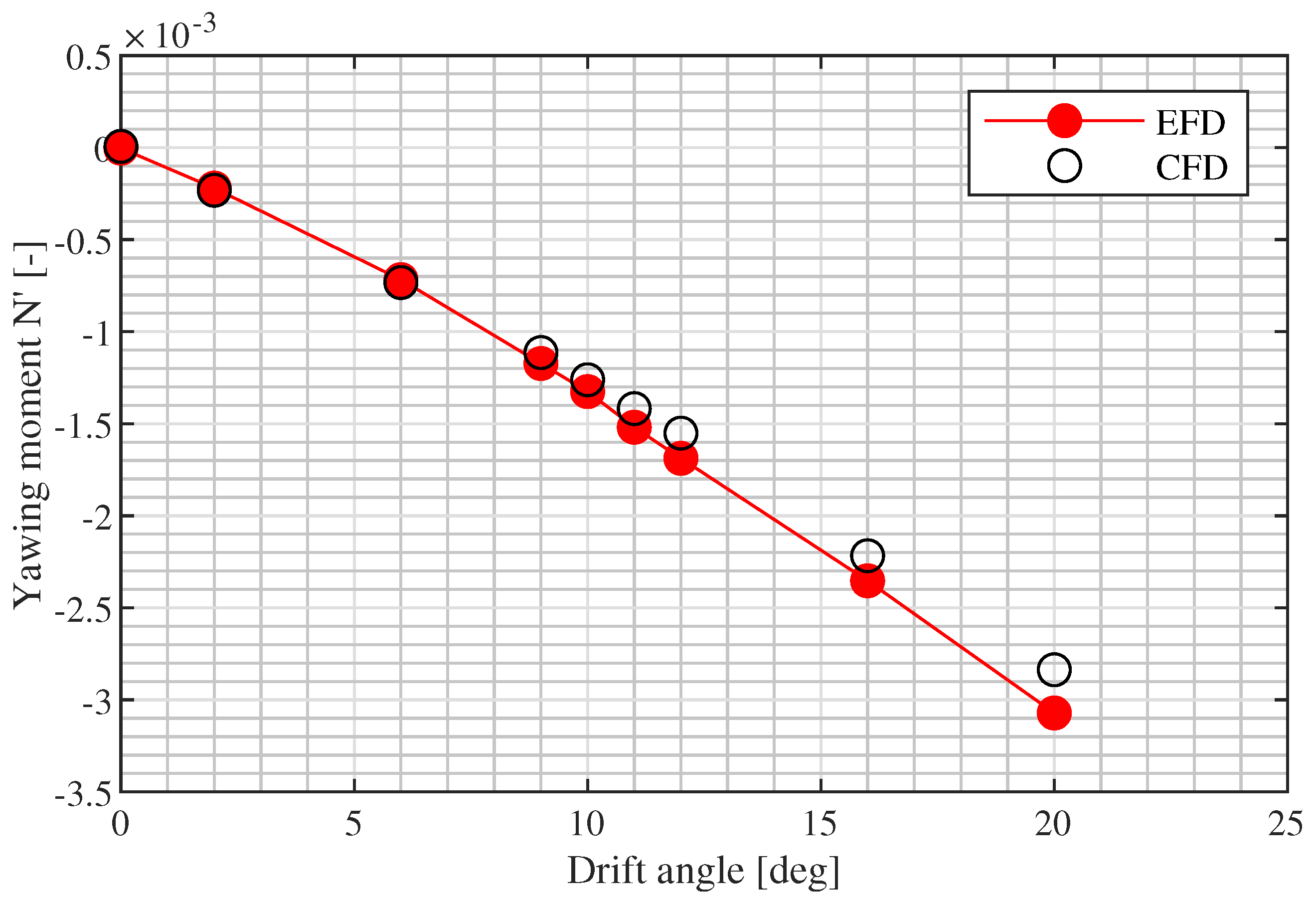
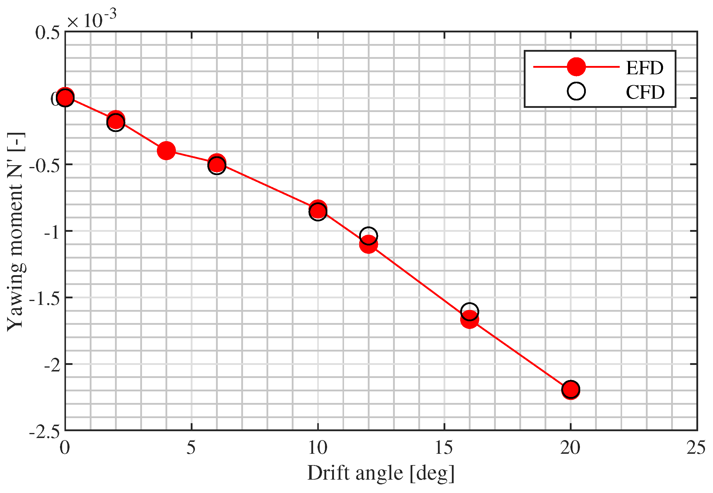
Figure 15.
Yawing moment N’ in the static drift tests-bare hull configuration.
Figure 15.
Yawing moment N’ in the static drift tests-bare hull configuration.
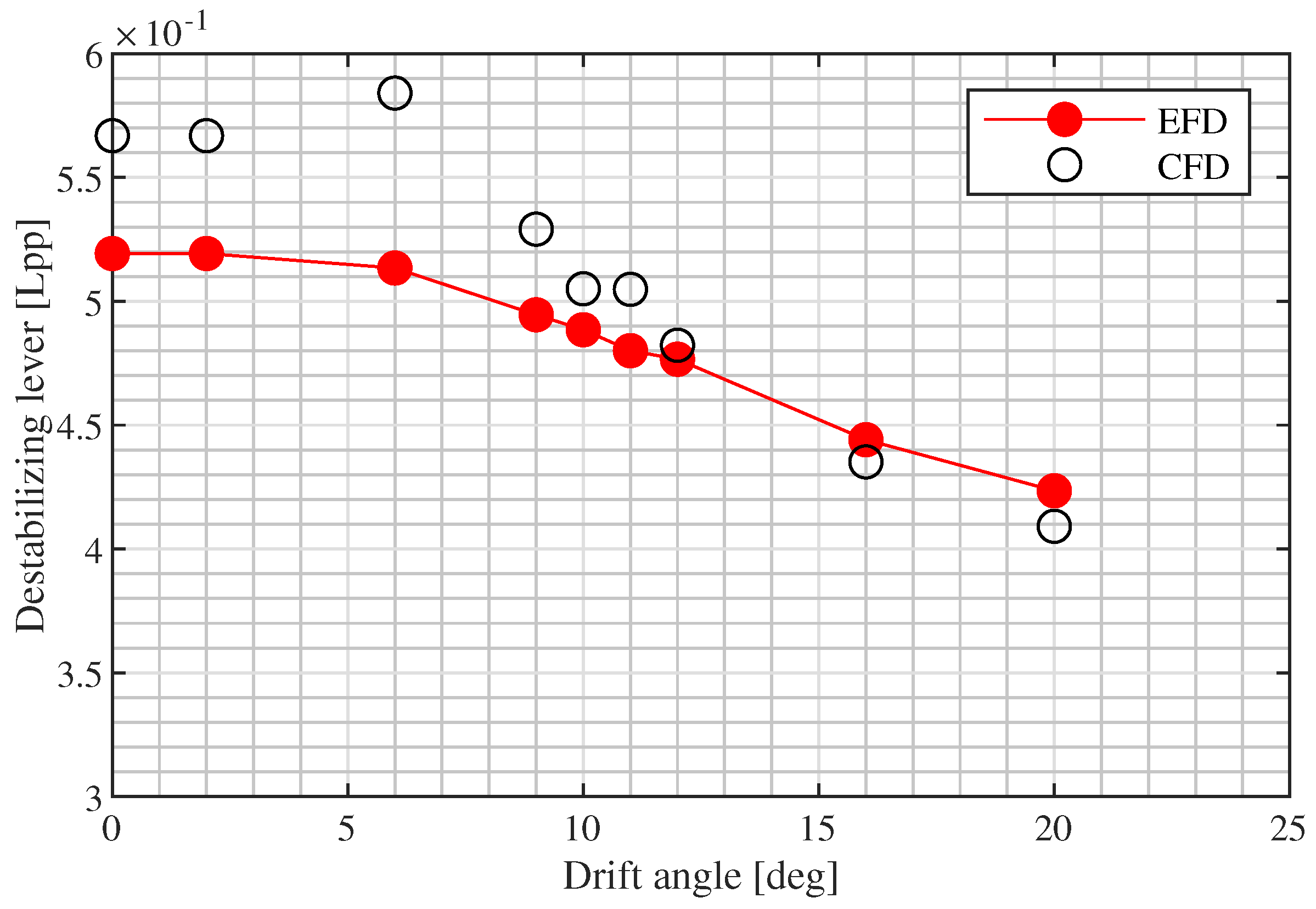
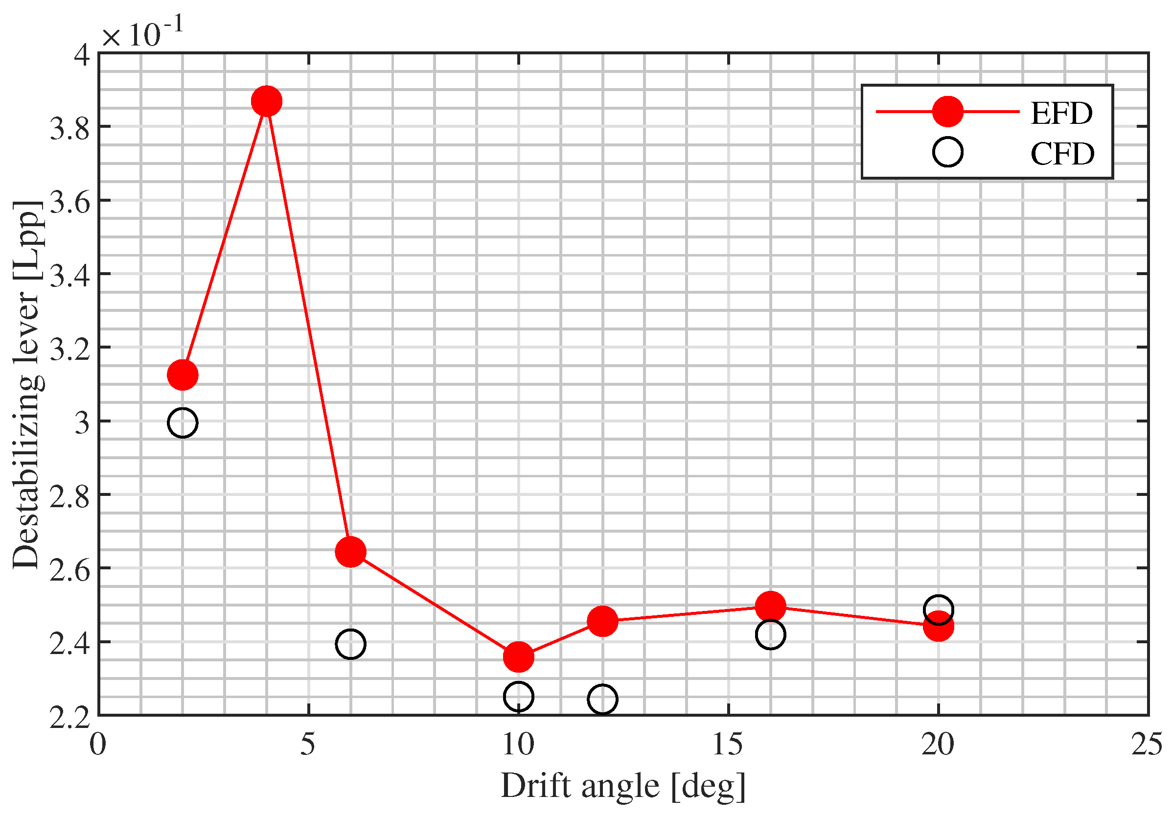
Figure 16.
Destabilizing lever in the static drift tests-bare hull configuration.
Figure 16.
Destabilizing lever in the static drift tests-bare hull configuration.
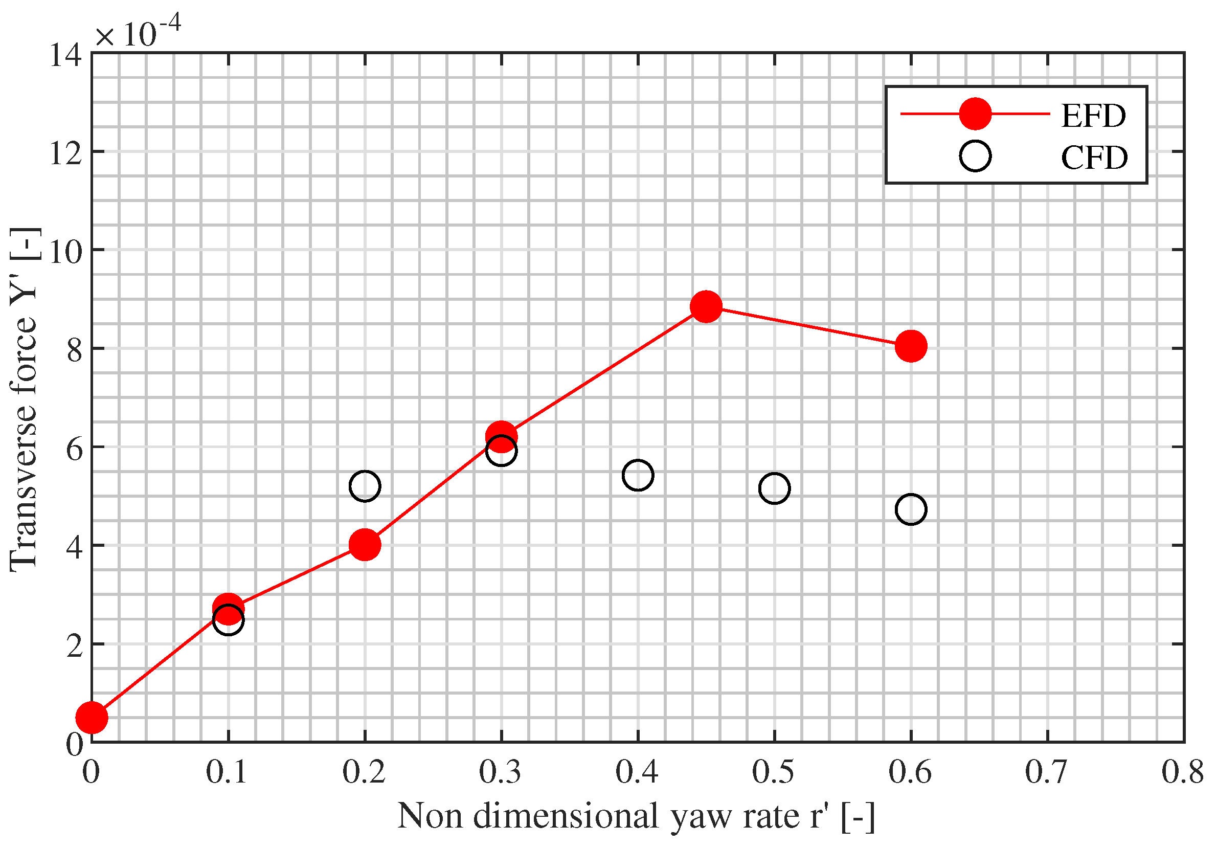
Figure 17.
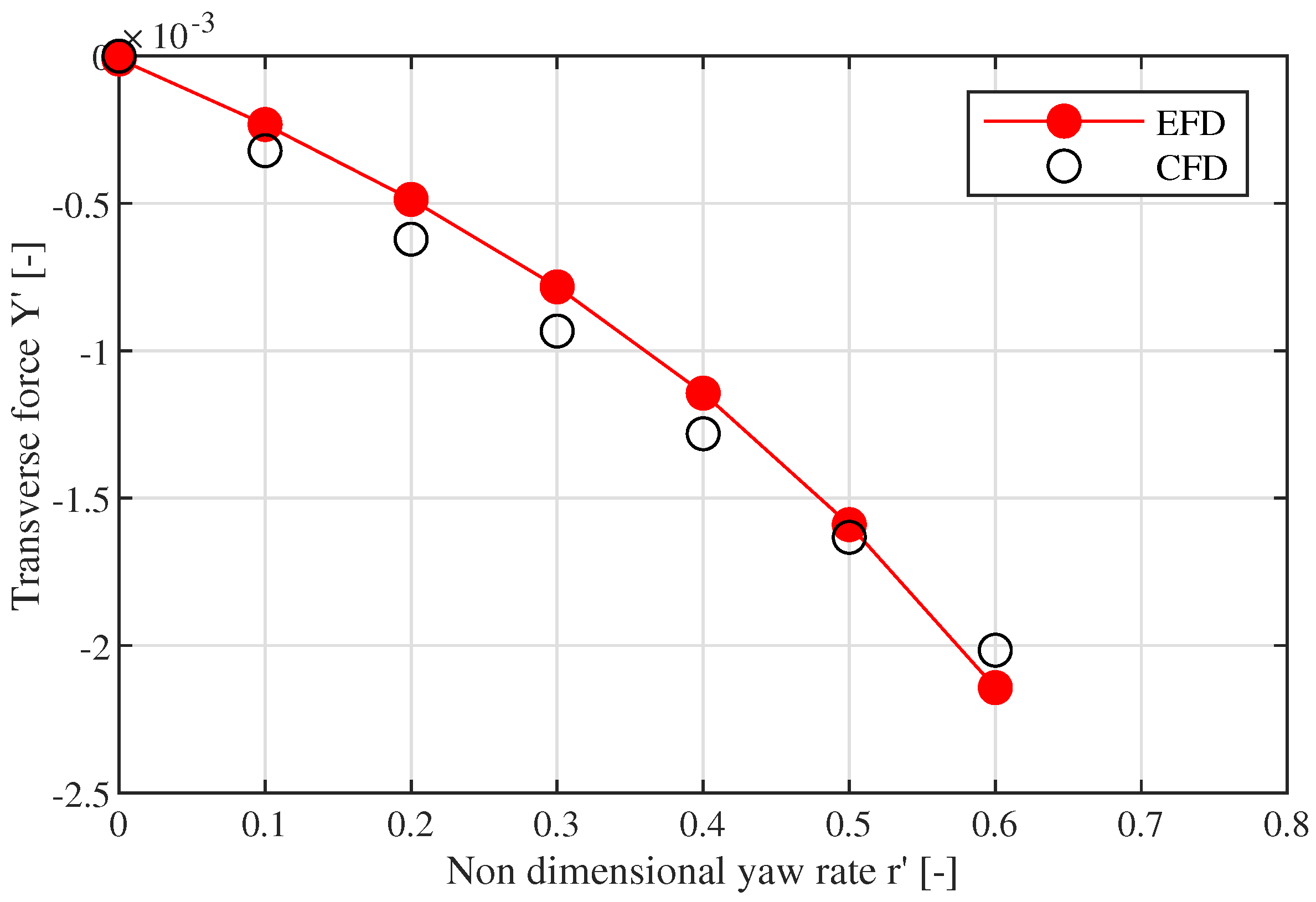
Transverse force in the static yaw rate tests-bare hull configuration.
Figure 17.
Transverse force in the static yaw rate tests-bare hull configuration.
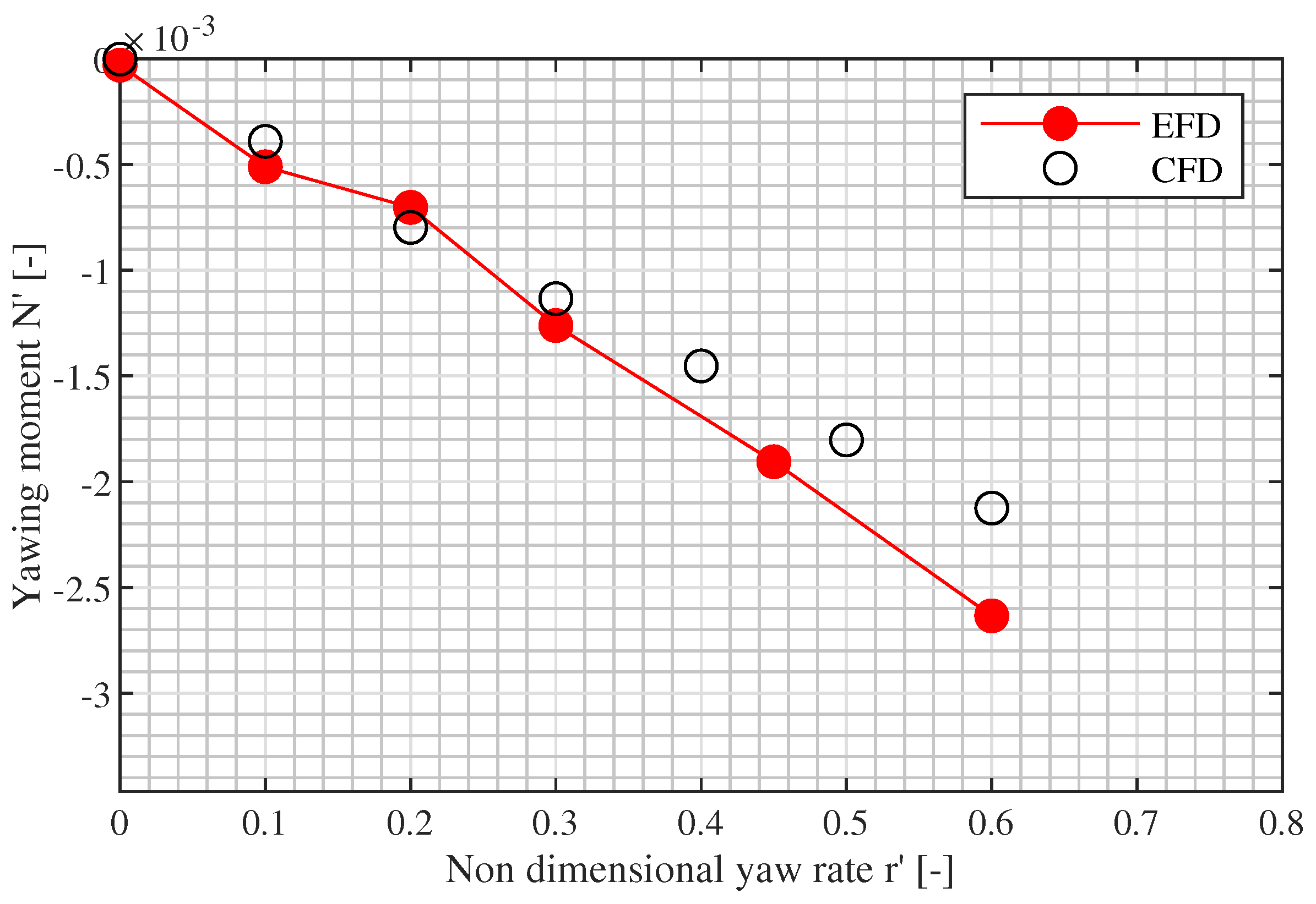
Figure 18.
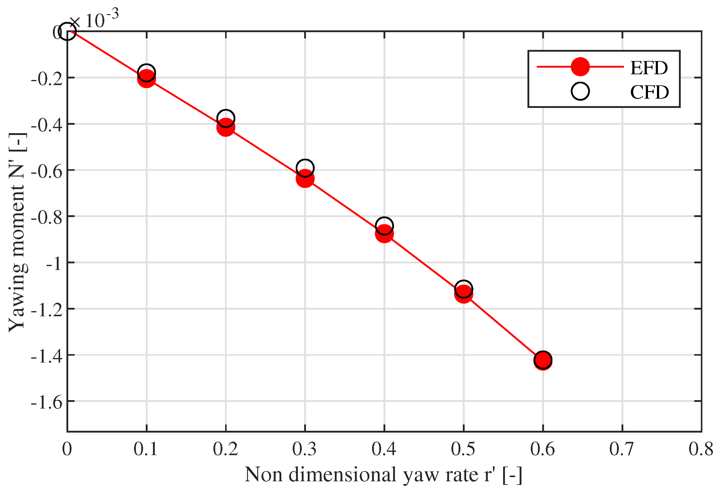
Yawing moment in the static yaw rate tests-bare hull configuration.
Figure 18.
Yawing moment in the static yaw rate tests-bare hull configuration.
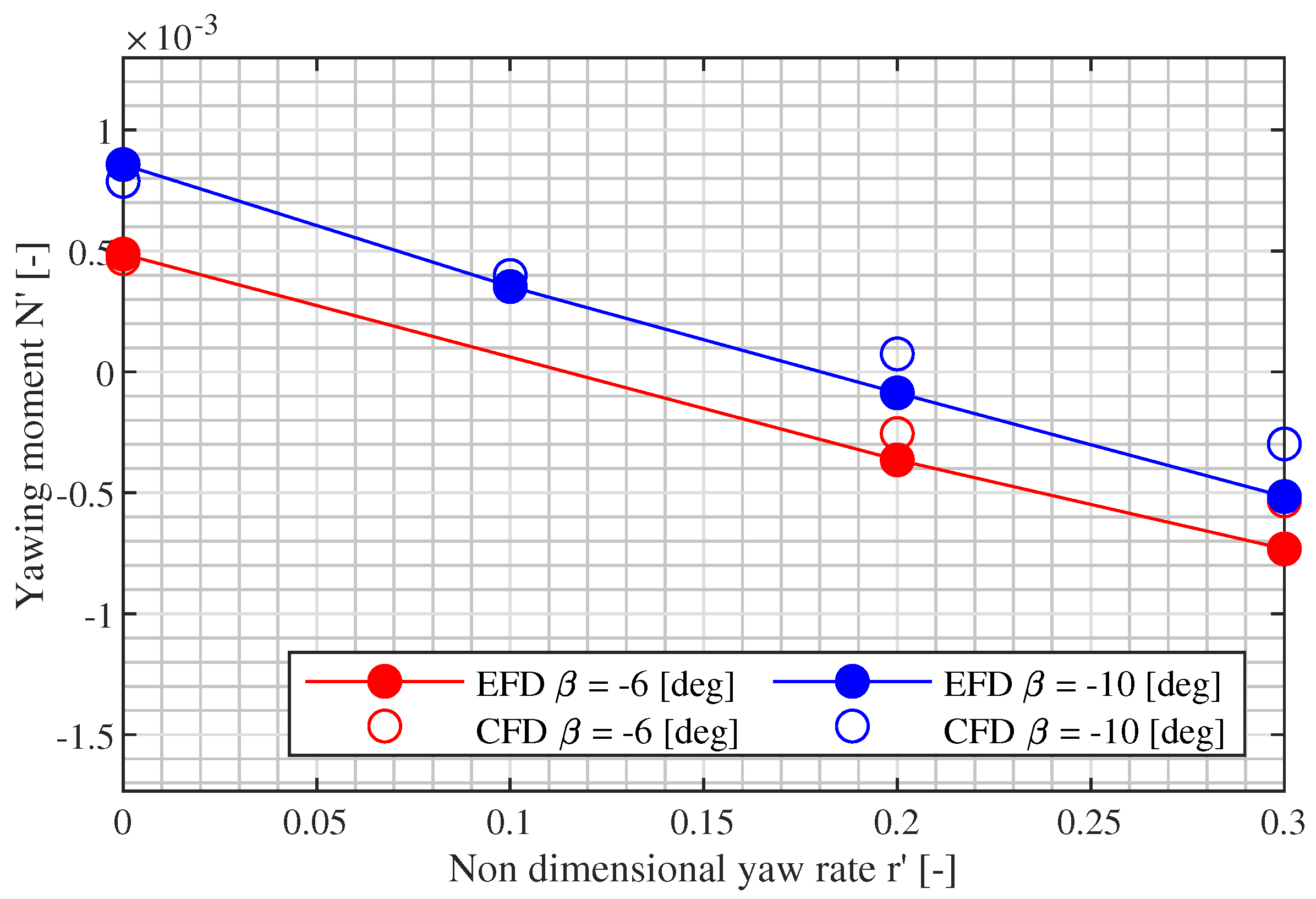
Figure 19.
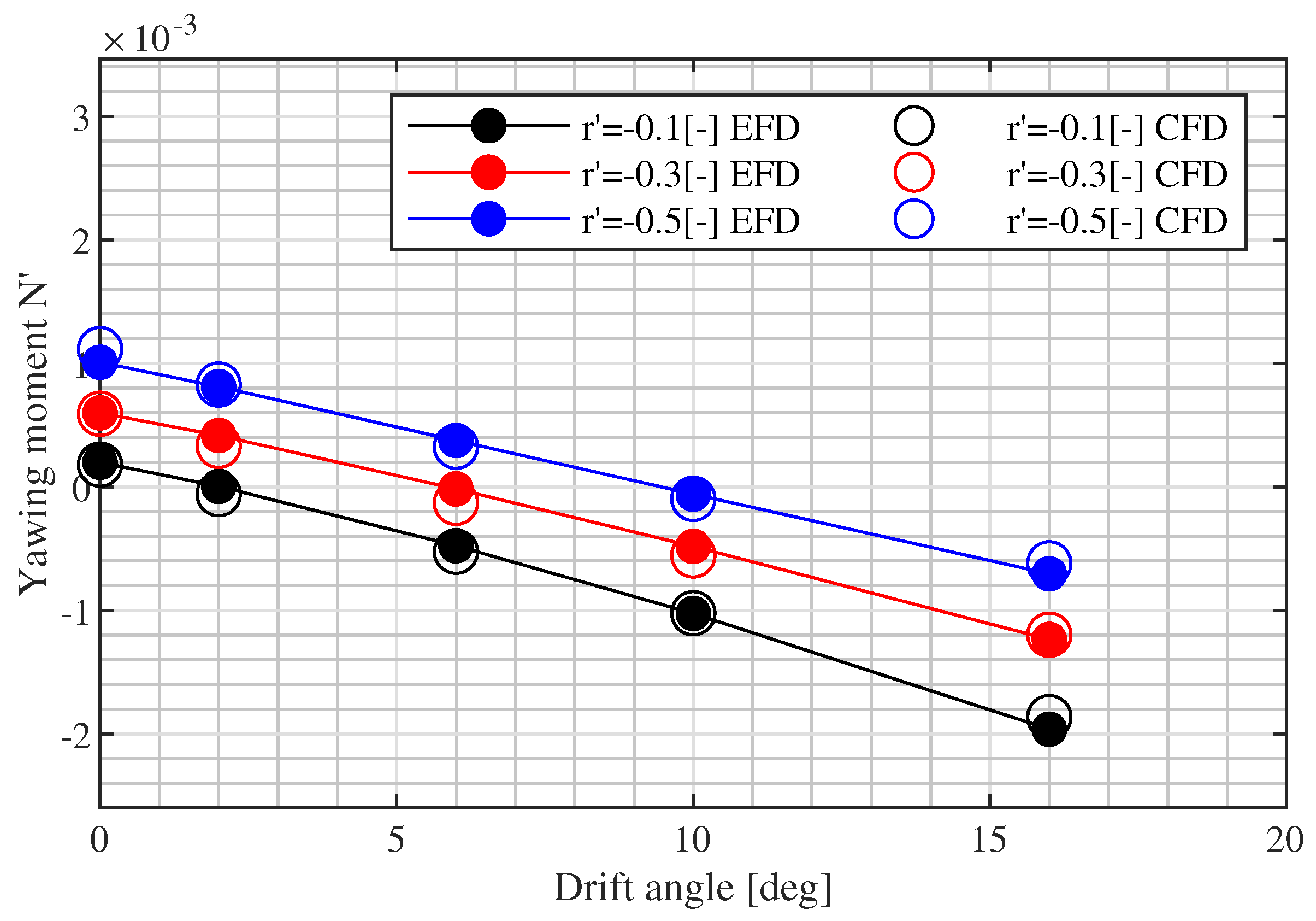
Yawing moment in the combined drift and yaw rate tests-bare hull configuration.
Figure 19.
Yawing moment in the combined drift and yaw rate tests-bare hull configuration.
Figure 20.
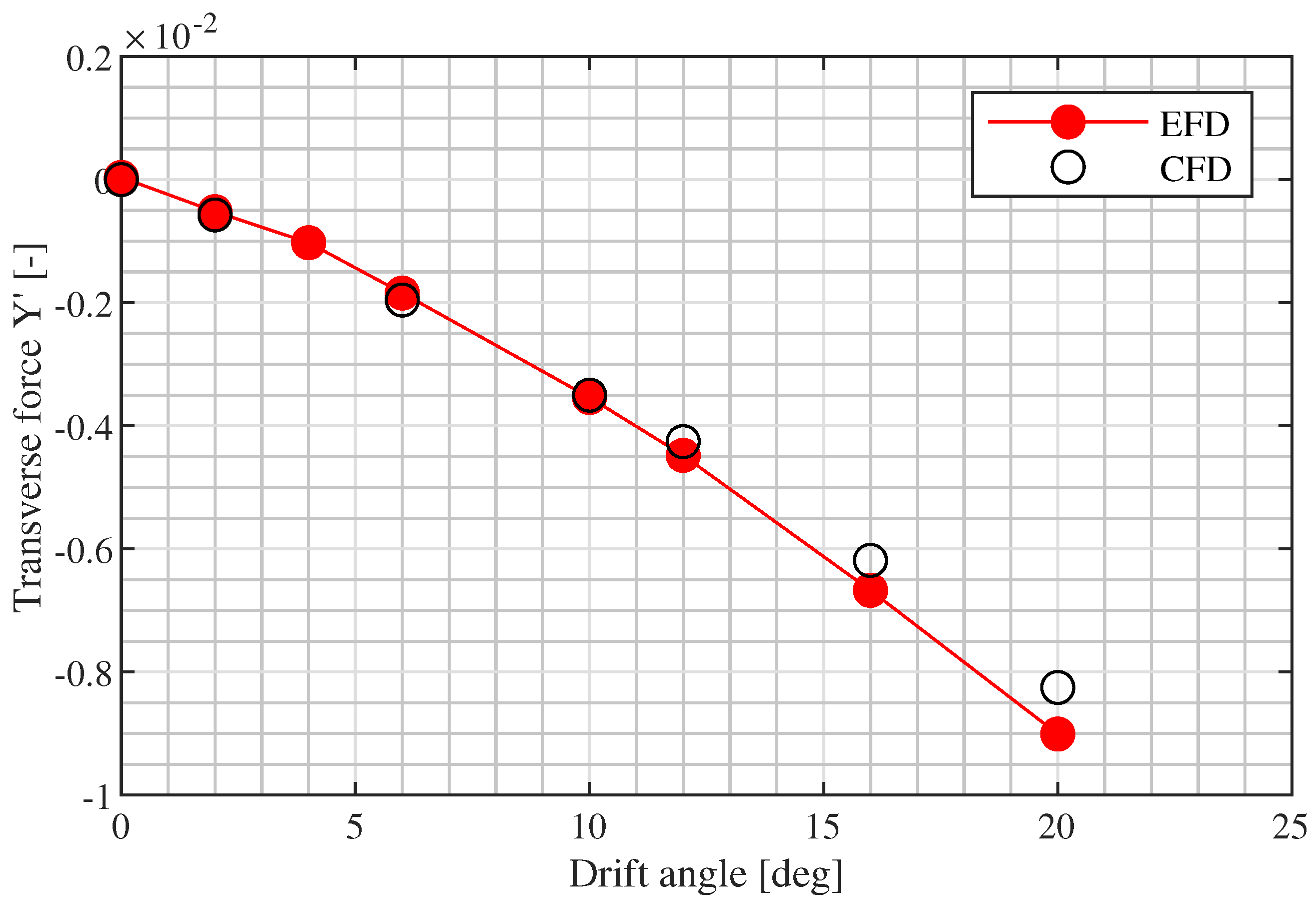
Transverse force Y’ in the static drift tests-fully appended configuration.
Figure 20.
Transverse force Y’ in the static drift tests-fully appended configuration.
Figure 21.
Yawing moment N’ in the static drift tests-fully appended configuration.
Figure 21.
Yawing moment N’ in the static drift tests-fully appended configuration.
Figure 22.
Destabilizing lever in the static drift tests-fully appended configuration.
Figure 22.
Destabilizing lever in the static drift tests-fully appended configuration.
Figure 23.
Transverse force in the static yaw rate tests-fully appended configuration.
Figure 23.
Transverse force in the static yaw rate tests-fully appended configuration.
Figure 24.
Yawing moment in the static yaw rate tests-fully appended configuration.
Figure 24.
Yawing moment in the static yaw rate tests-fully appended configuration.
Figure 25.
Yawing moment in the combined tests-fully appended configuration.
Figure 25.
Yawing moment in the combined tests-fully appended configuration.
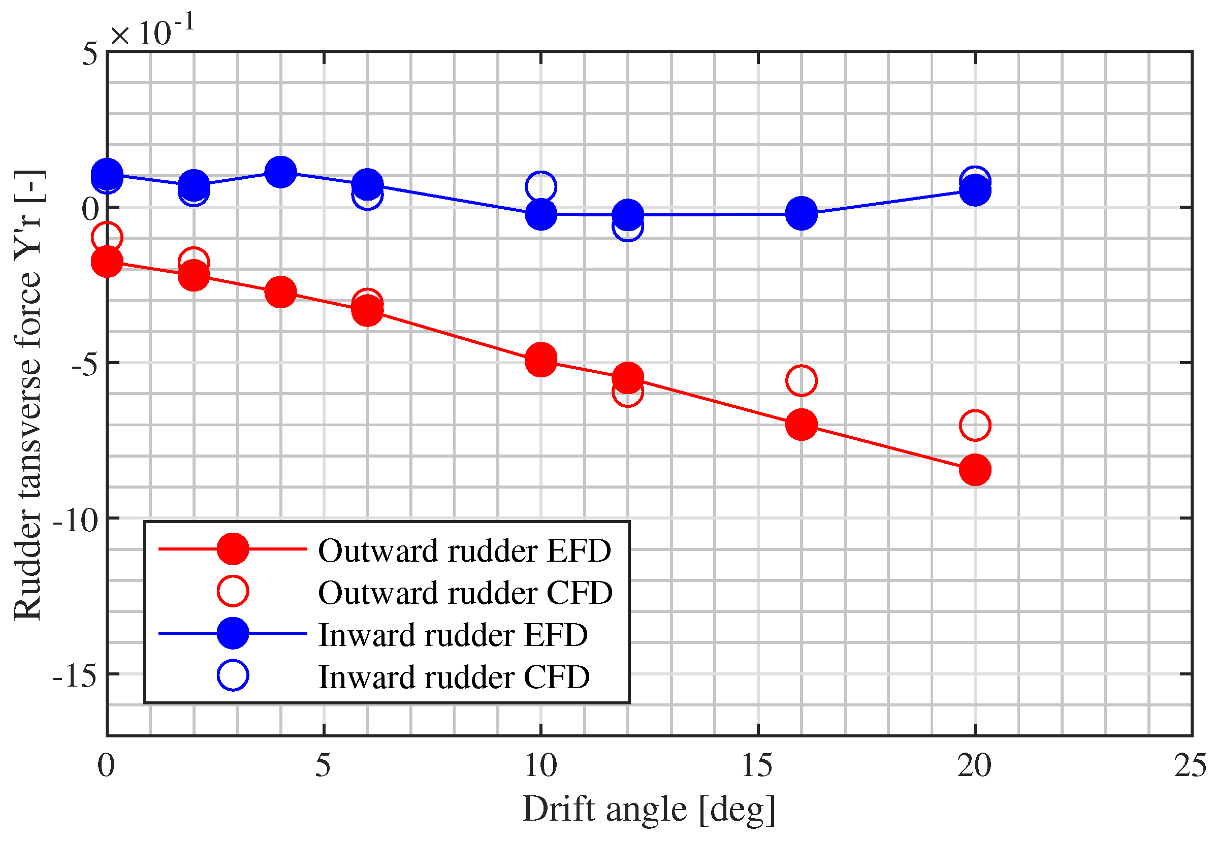
Figure 26.
Rudder transverse force in the static drift tests.
Figure 26.
Rudder transverse force in the static drift tests.
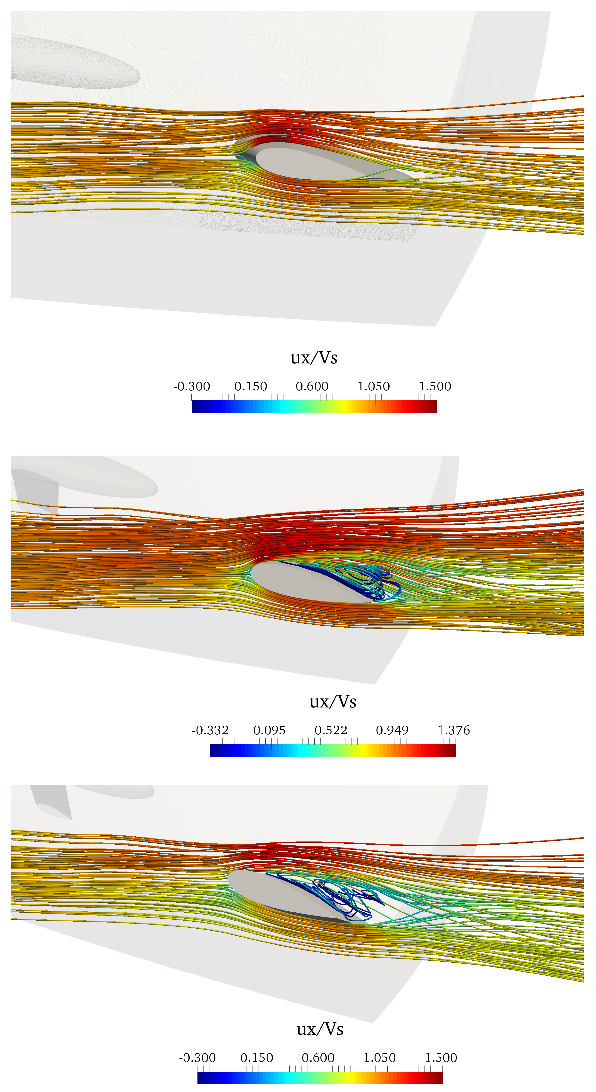
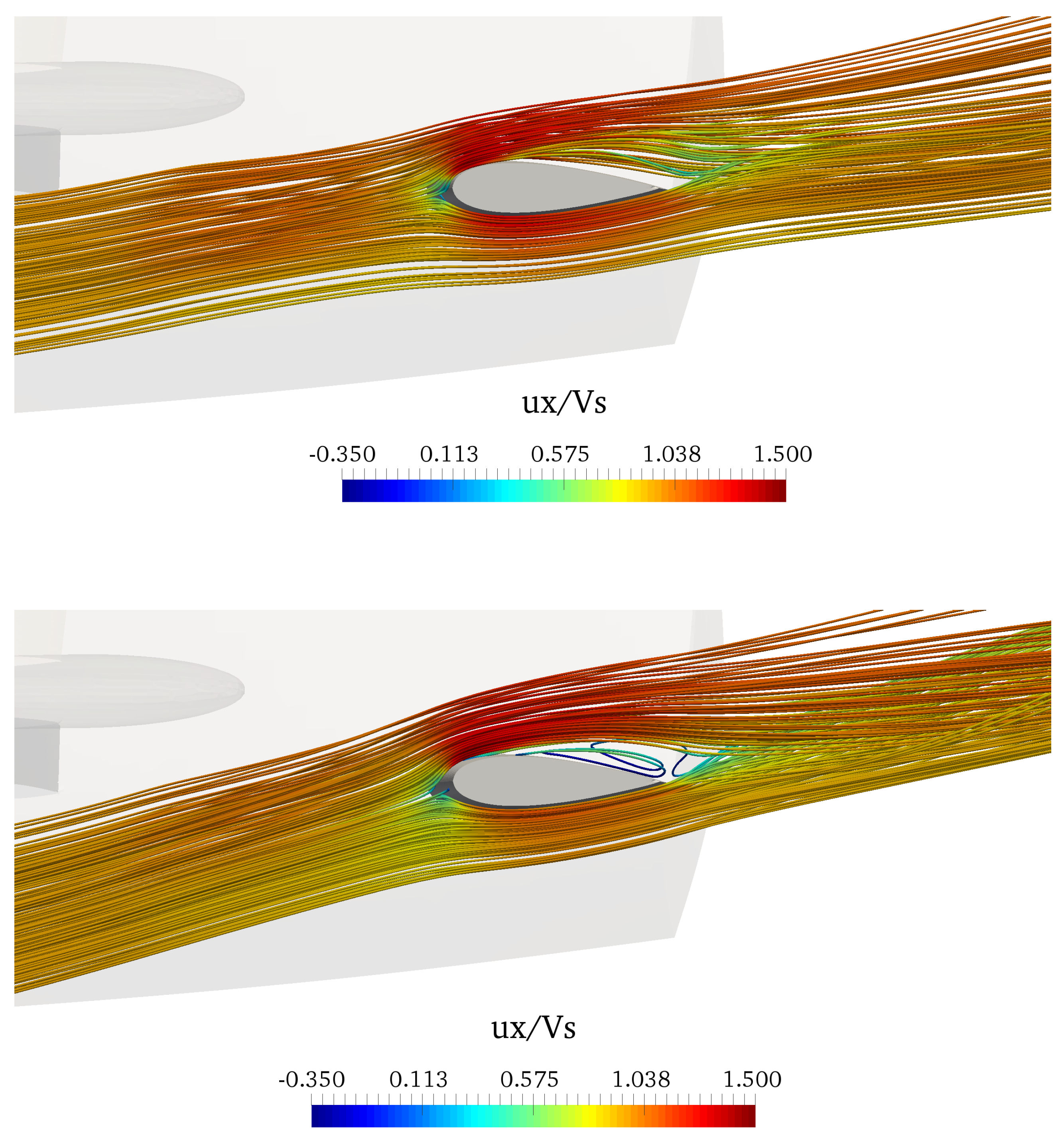
Figure 27.
Rudder streamlines in the pure drift tests = 10 [deg], = 16 [deg] and = 20 [deg].
Figure 27.
Rudder streamlines in the pure drift tests = 10 [deg], = 16 [deg] and = 20 [deg].
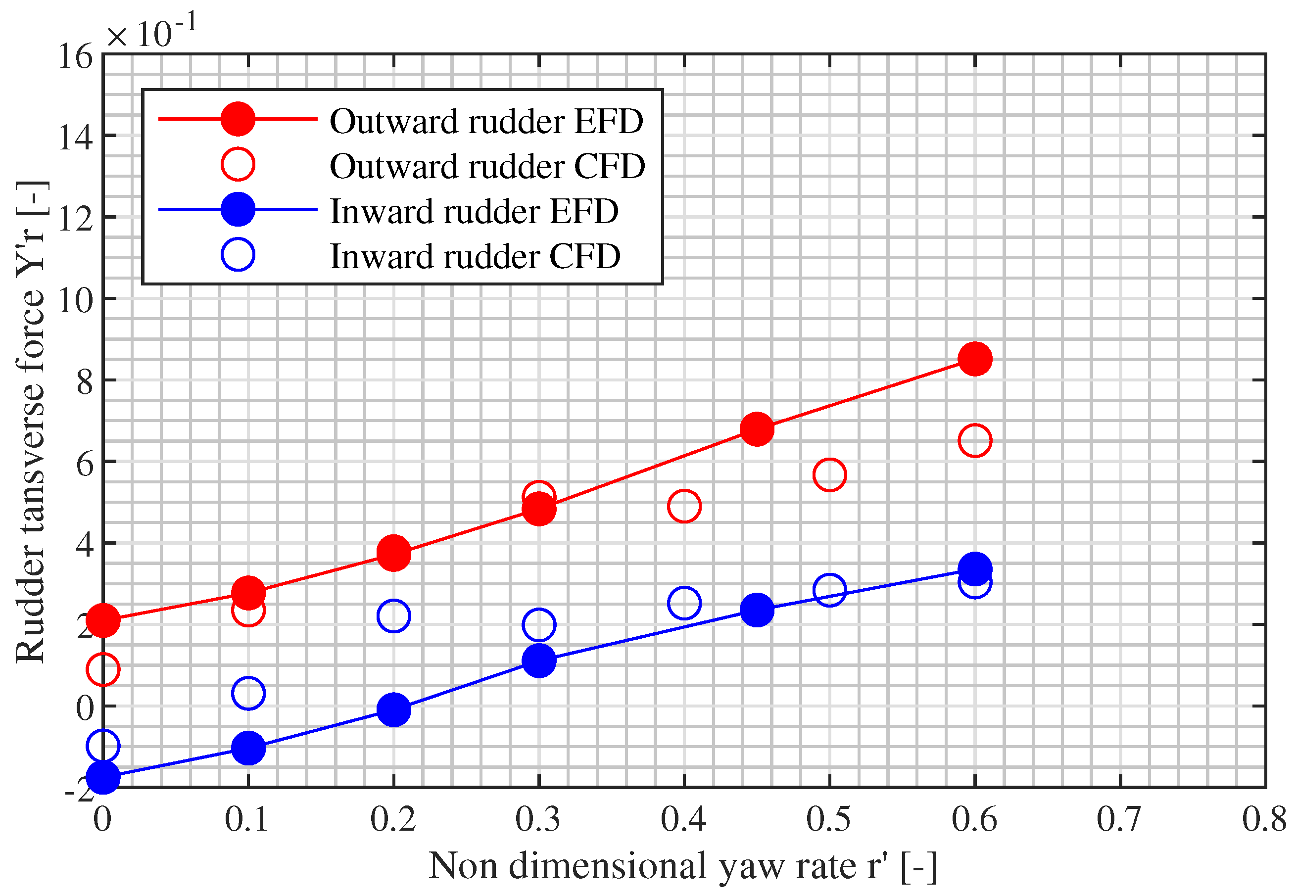
Figure 28.
Ruddertransverse force in the static yaw rate tests.
Figure 28.
Ruddertransverse force in the static yaw rate tests.
Figure 29.
Rudder stall in the rotation tests r’ = 0.3 [−] and r’ = 0.6 [−].
Figure 29.
Rudder stall in the rotation tests r’ = 0.3 [−] and r’ = 0.6 [−].
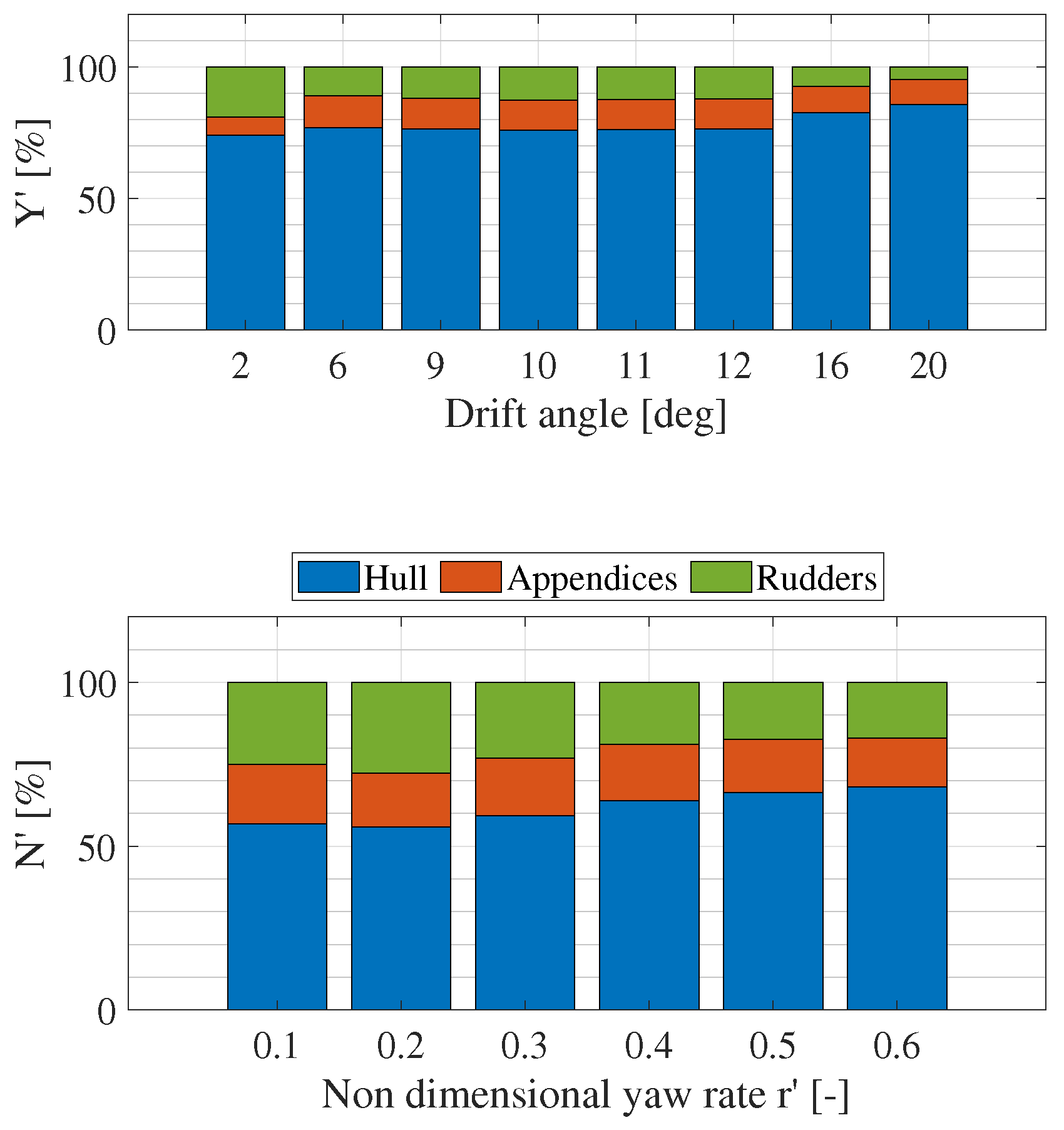
Figure 30.
Percentage of the global force produced by the hull, appendices and rudders.
Figure 30.
Percentage of the global force produced by the hull, appendices and rudders.
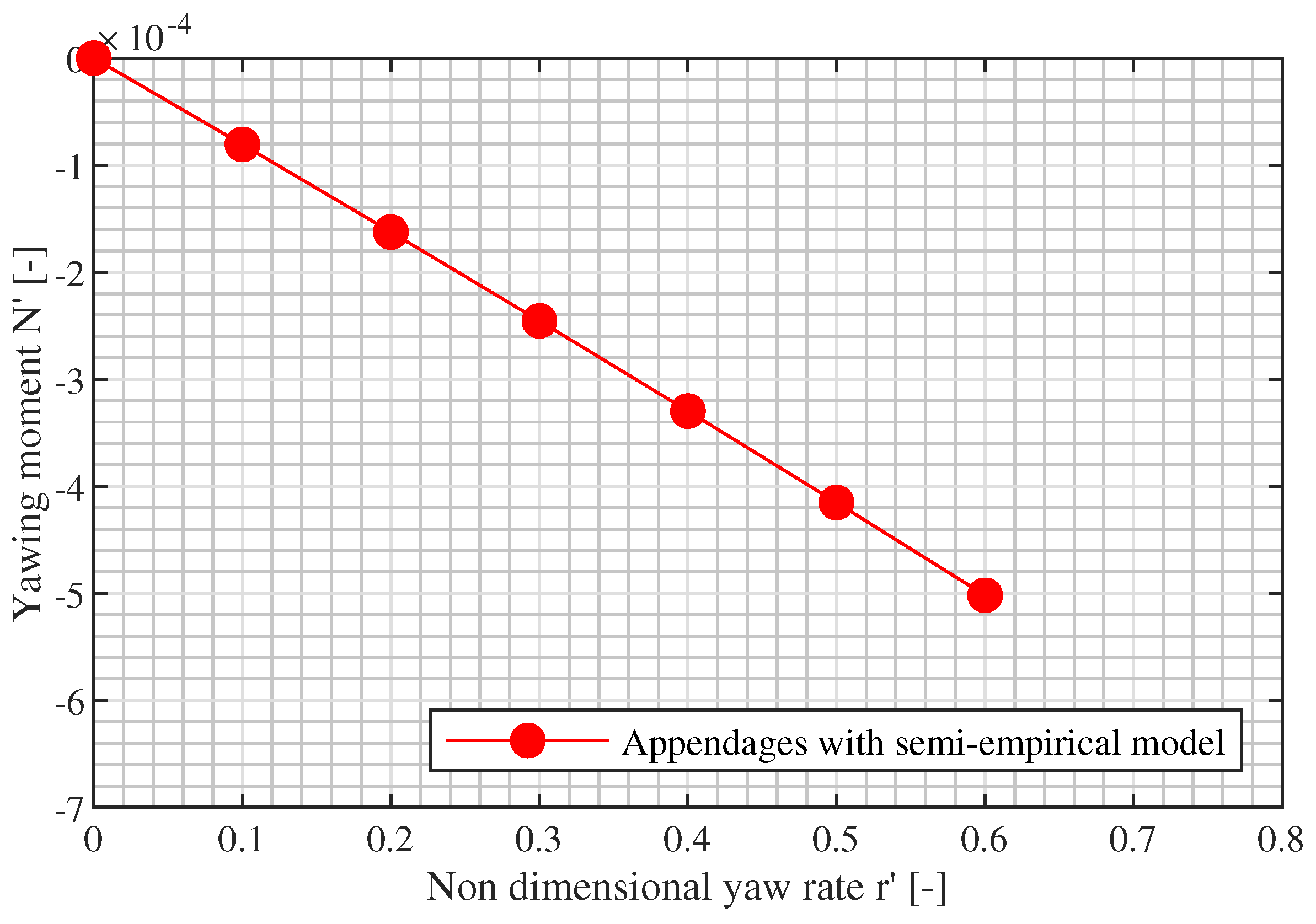
Figure 31.
N’ of the appendages in the rotation tests by means of semi-empirical models.
Figure 31.
N’ of the appendages in the rotation tests by means of semi-empirical models.
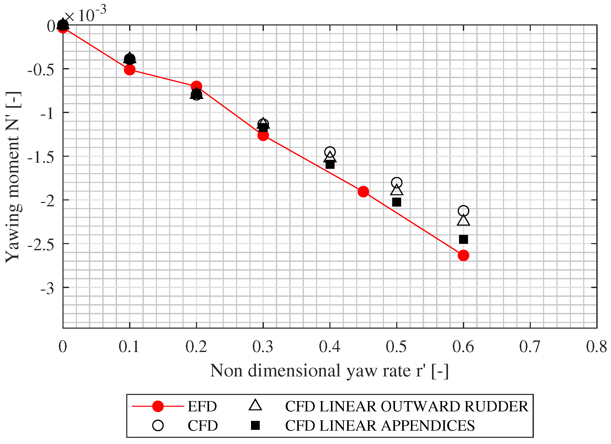
Figure 32.
N’ in the rotation tests with linear contribution of the appendices.
Figure 32.
N’ in the rotation tests with linear contribution of the appendices.
Figure 33.
Zig-zag = trajectory.
Figure 33.
Zig-zag = trajectory.
Figure 34.
Turning circle = trajectory.
Figure 34.
Turning circle = trajectory.
Figure 35.
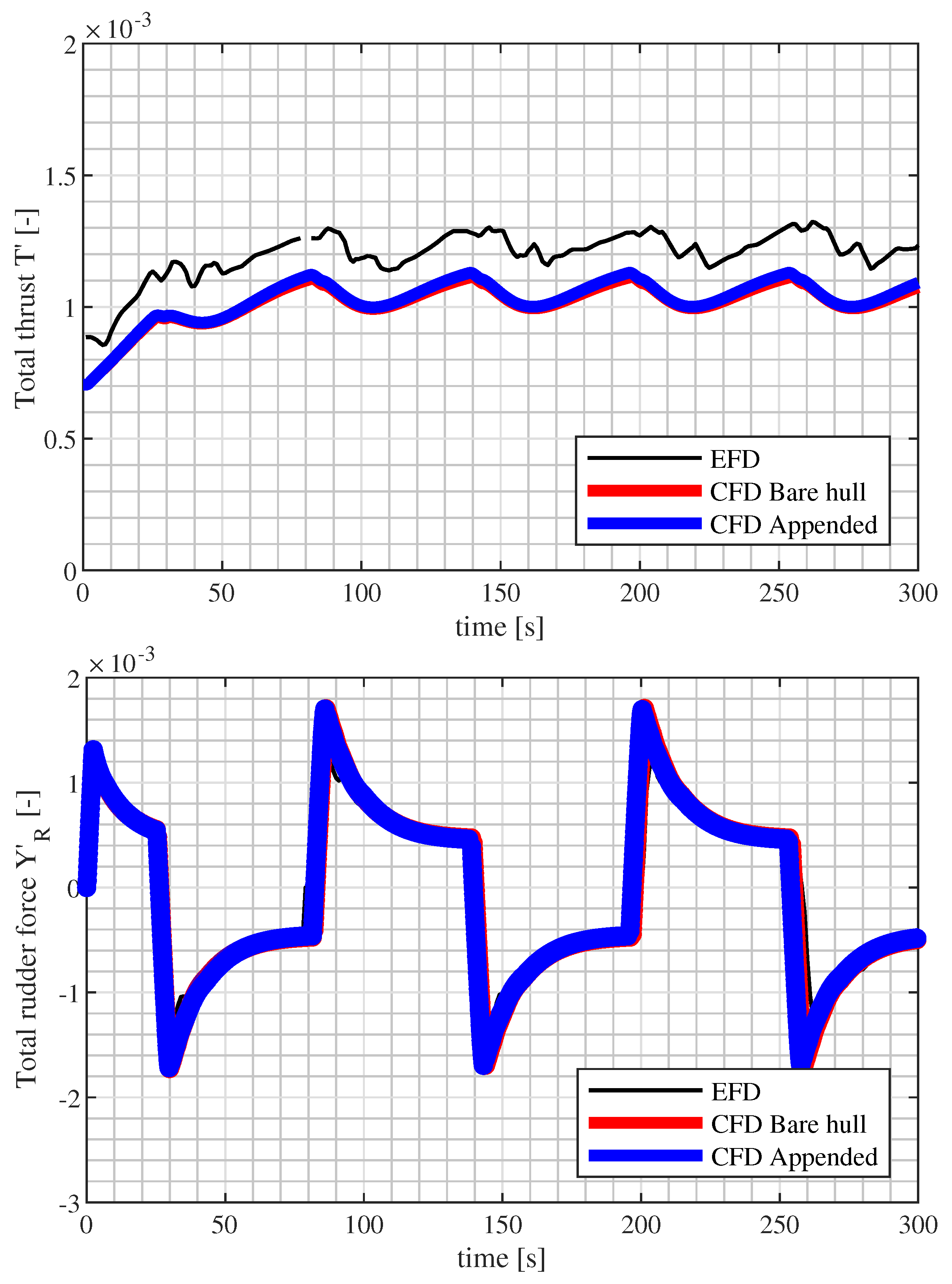
Thrust and rudder total forces time traces in zig zag 20/20.
Figure 35.
Thrust and rudder total forces time traces in zig zag 20/20.
Figure 36.
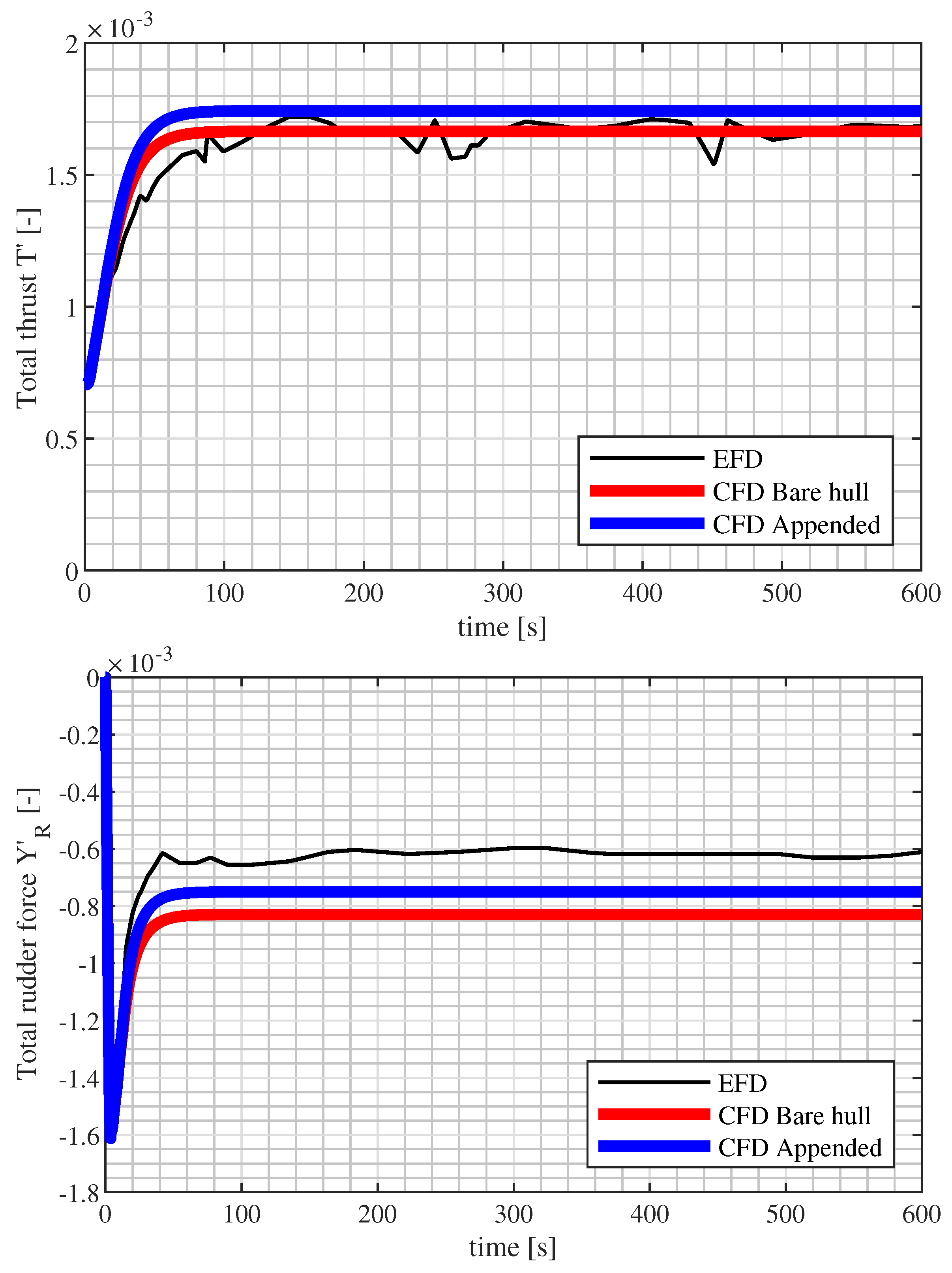
The thrust and rudder total force time traces in a turning circle.
Figure 36.
The thrust and rudder total force time traces in a turning circle.
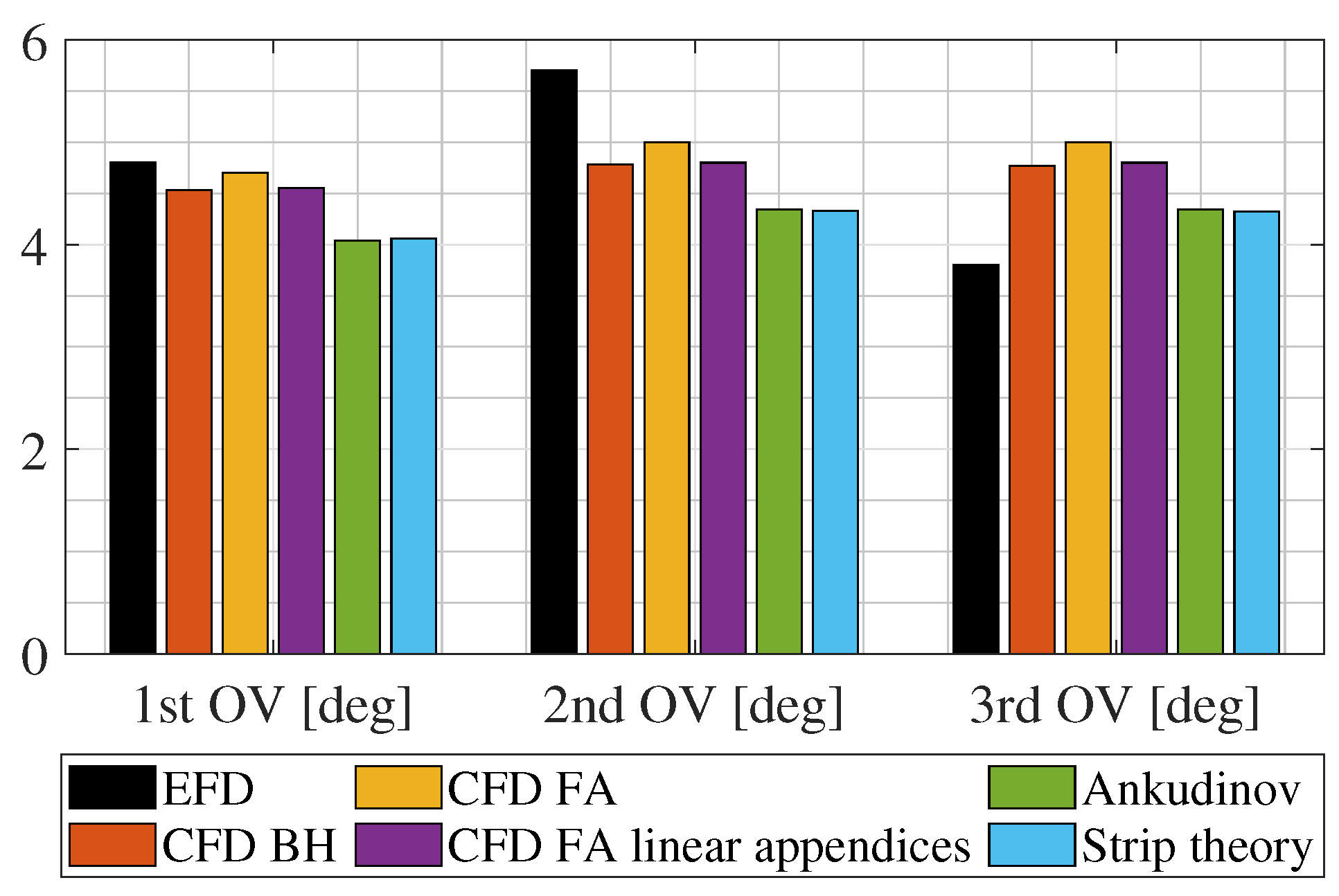
Figure 37.
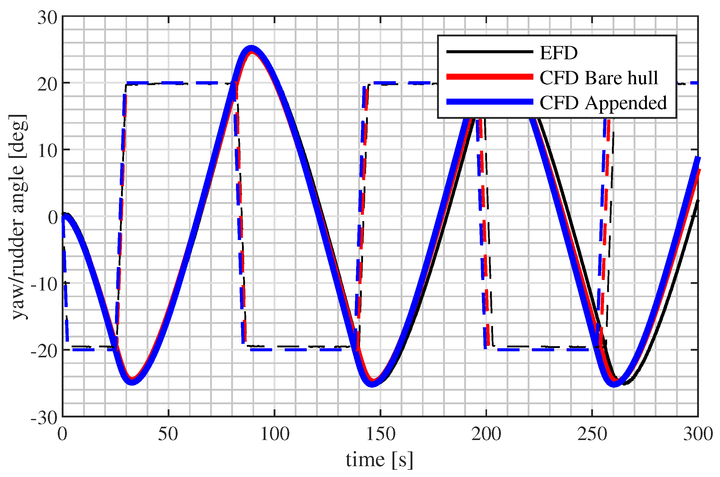
The Zig-Zag / manoeuvre characteristics.
Figure 37.
The Zig-Zag / manoeuvre characteristics.
Figure 38.
The Zig-Zag / manoeuvre characteristics.
Figure 38.
The Zig-Zag / manoeuvre characteristics.
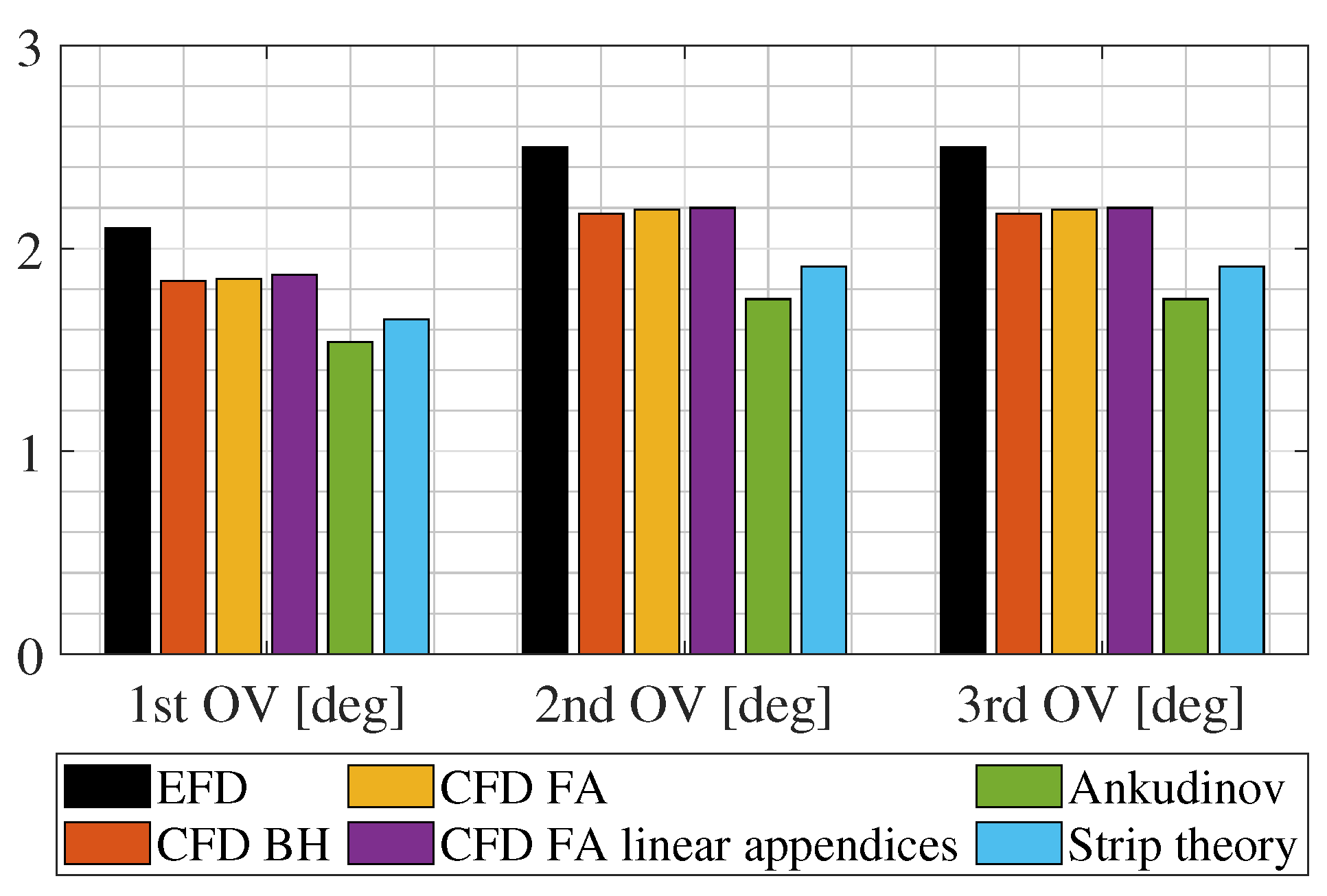
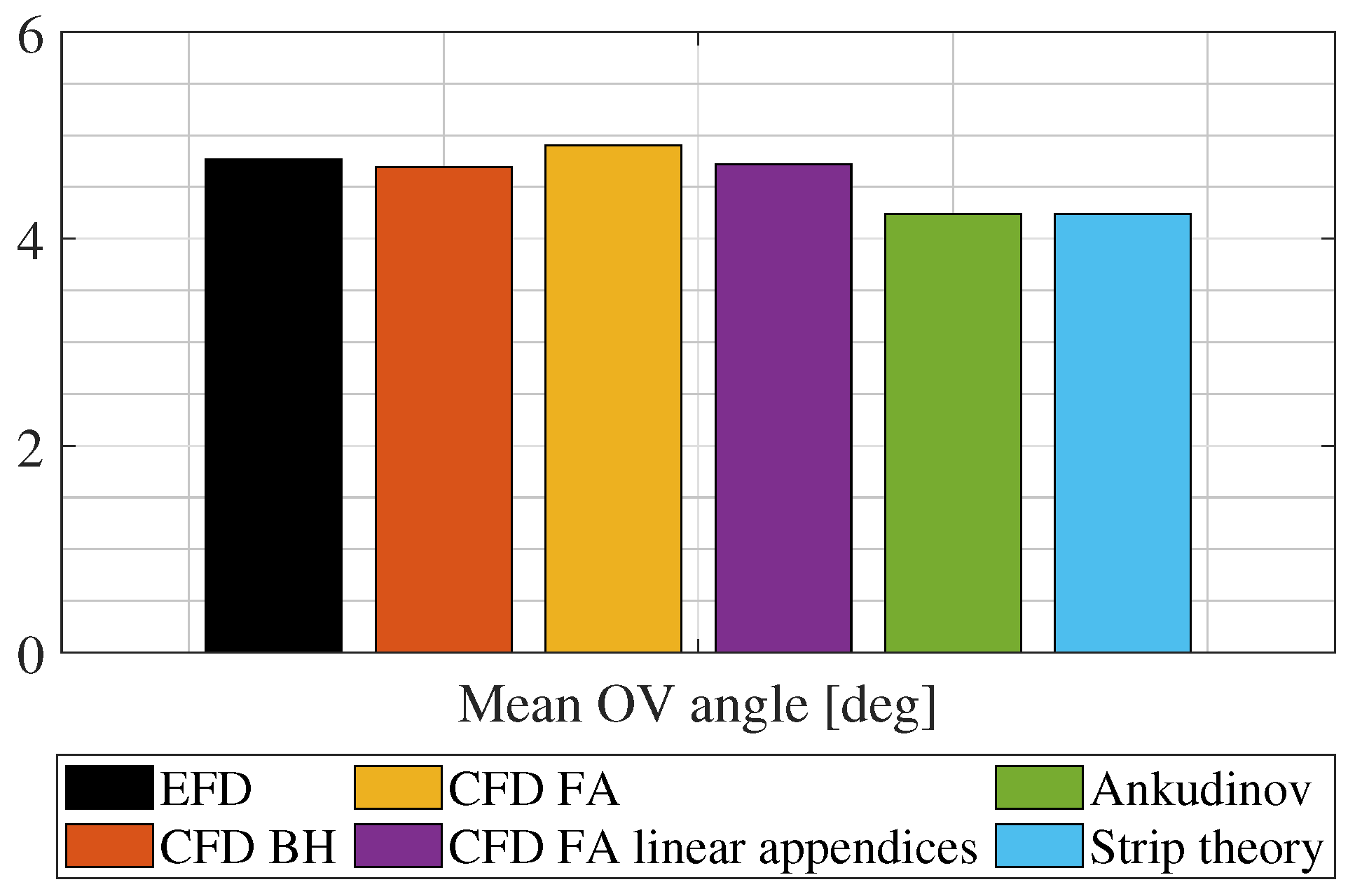
Figure 39.
The Zig-Zag / mean overshoot angles.
Figure 39.
The Zig-Zag / mean overshoot angles.
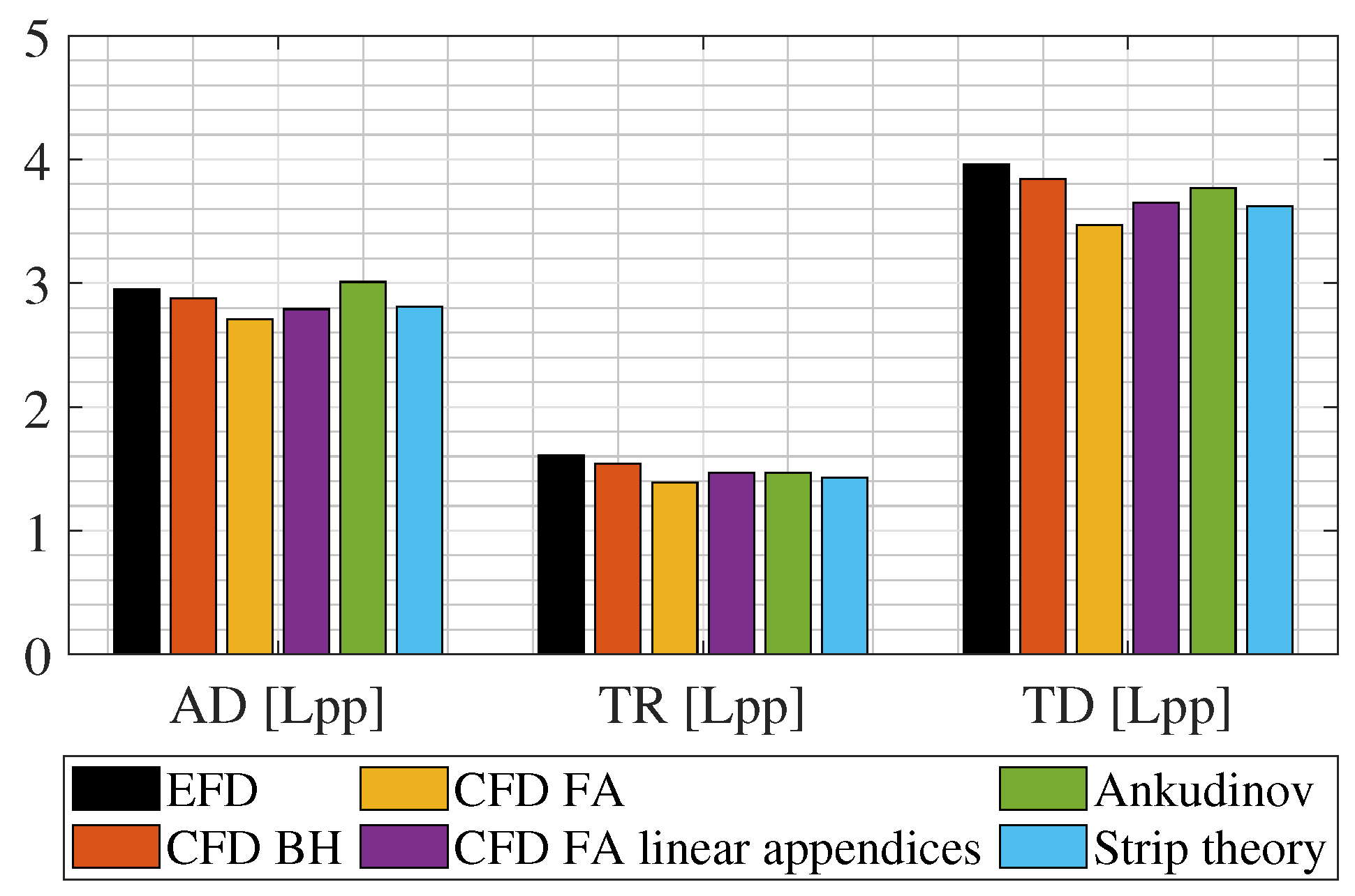
Figure 40.
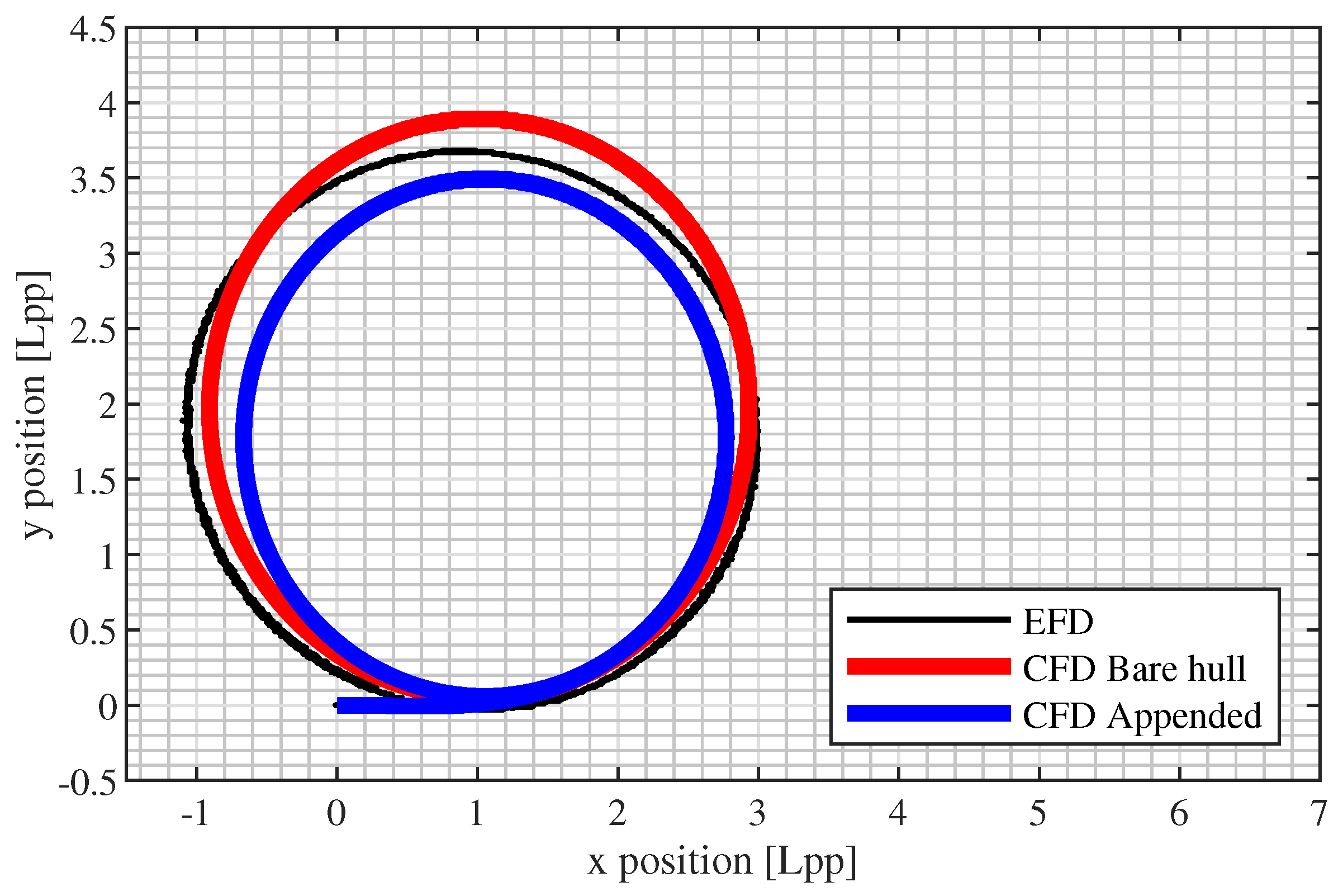
The Turning circle = manoeuvre characteristics.
Figure 40.
The Turning circle = manoeuvre characteristics.
Table 1.
OpenFoam domain dimensions.
Table 1.
OpenFoam domain dimensions.
| Computational Domain Dimensions |
|---|
| [] | 4.5 |
| [] | 2.5 |
| [] | 2 |
Table 2.
Richardson analysis data.
Table 2.
Richardson analysis data.
| Richardson Mesh Convergence Analysis |
|---|
| Mesh | Fine | Standard | Coarse |
| 1/ | 1 | |
| h | 1.77 | 1.59 | 1.42 |
| 0.90 |
| 0.89 |
| Drift test |
| Longitudinal force X’ |
| Value | –1.35 × | –1.36 × | –1.80 × |
| Convergence | Monotonic |
| 0.3 |
| Transverse force Y’ |
| Value | 7.11 × | 6.98 × | 6.95 × |
| Convergence | Monotonic |
| 0.62 |
| Yawing moment N’ |
| Value | 2.81 × | 2.86 × | 2.89 × |
| Convergence | Monotonic |
| 2.2 |
| Rotation test |
| Longitudinal force X’ |
| Value | –1.07 × | –1.08 × | –1.09 × |
| Convergence | Monotonic |
| 5.0 |
| Transverse force Y’ |
| Value | –2.05 × | –2.03 × | –1.92 × |
| Convergence | Monotonic |
| 0.4 |
| Yawing moment N’ |
| Value | –1.43 × | –1.44 × | –1.49 × |
| Convergence | Monotonic |
| 0.1 |
Table 3.
Mesh and fluid characteristics in the bare hull calculations.
Table 3.
Mesh and fluid characteristics in the bare hull calculations.
| Mesh Characteristics |
|---|
| Description | cartesian |
| Type of grid | unstructured |
| Number of cells | 1.5 M |
| y+ on the hull | 15 |
| Stretching ratio | 1.2 |
| Number of surface elements | 200 k |
| Fluid properties |
| Density [kg/m] | 1000 |
| Kinematic viscosity [m/s] | 1 × 10 |
| Reynolds number | 4.3 × 10 |
| Froude number | 0.280 |
Table 4.
Numerical schemes.
Table 4.
Numerical schemes.
| Numerical Schemes |
|---|
| ddtSchemes | localEuler |
| gradSchemes | Gauss linear |
| divSchemes | Gauss linearUpwind |
| laplacianSchemes | Gauss linear |
| interpolationSchemes | linear |
| snGradSchemes | limited |
Table 5.
Mesh characteristics in the appended calculations.
Table 5.
Mesh characteristics in the appended calculations.
| Mesh Characteristics |
|---|
| Description | cartesian |
| Type of grid | unstructured |
| Number of cells | 5.3 M |
| y+ on the hull | 1.6 |
| Stretching ratio | 1.2 |
| Number of surface elements | 300 k |
Table 6.
The DTMB 5415 test case.
Table 6.
The DTMB 5415 test case.
| Test Case |
|---|
| Description | Unit | Value |
| m | 142.0 |
| B | m | 19.0 |
| T | m | 6.14 |
| m | 71.60 |
| kn | 18.0 |
| Fr | - | 0.248 |
Table 7.
The model characteristics.
Table 7.
The model characteristics.
| Characteristics of the Models |
|---|
| Quantity | SHIP | INSEAN | FORCE | MARIN |
| [−] | 1 | 24.83 | 35.48 | 35.48 |
| [m] | 142 | 5.72 | 4.00 | 4.00 |
| B [m] | 19 | 0.768 | 0.537 | 0.537 |
| T [m] | 6.14 | 0.248 | 0.173 | 0.173 |
| ∇ [m] | 8.5k | 0.554 | 0.189 | 0.189 |
| Fr [−] | - | 0.138, 0.280, 0.410 | 0.138, 0.280, 0.410 | 0.248, 0.410 |
| [kn] | - | 10.0, 20.0, 30.0 | 10.0, 20.0, 30.0 | 18.0, 30.0 |
| Configuration | - | 5415 | 5415 | 5415 M |
Table 8.
The geometric characteristics of the appendices.
Table 8.
The geometric characteristics of the appendices.
| Geometric Characteristics of the Appendices |
|---|
| Ship scale |
| Rudder headbox |
| Span [m] | 1.2 |
| Chord [m] | 4.4 |
| Skeg |
| Lateral area [m] | 12.3 |
| Shaft |
| Length [m] | 24.1 |
| Diameter [m] | 0.55 |
| Internal brackets |
| Span [m] | 4.0 |
| Chord [m] | 1.3 |
| External brackets |
| Span [m] | 3.3 |
| Chord [m] | 1.4 |
Table 9.
The geometric characteristics of the rudders.
Table 9.
The geometric characteristics of the rudders.
| Rudders |
|---|
| Ship scale |
| [m] | 4.4 |
| [m] | 3.5 |
| [m] | 0.89 |
| Point of max. thickness [%] | 25 |
| (each) [m] | 15.4 |
| Total rudders area ratio [%] | 3.62 |
| Angle in Y-Z plane [deg] | 15 |
Table 10.
The geometric characteristics of the propellers.
Table 10.
The geometric characteristics of the propellers.
| Propellers |
|---|
| Ship scale |
| [m] | 6.15 |
| [m] | 5.35 |
| [−] | 0.87 |
| Boss diameter ratio [−] | 0.347 |
| [−] | 0.580 |
| 5 |
| Direction of rotation | Inward over the top |
Table 11.
Experimental test matrix on 5415.
Table 11.
Experimental test matrix on 5415.
| EFD Test Matrix on 5415 Model |
|---|
| Fr = 0.280 [−] |
| Drift angle [deg] | Non dimensional yaw rate r’ [−] |
| Static drift tests |
| 0, 2, 6, 9, 10, 11, 12, 16, 20 | 0 |
| Rotation tests |
| 0 | 0.05, 0.15, 0.2, 0.3, 0.45, 0.6 |
| Drift and rotation tests |
| 9, 10, 11 | 0.3 |
Table 12.
Experimental test matrix on 5415 M.
Table 12.
Experimental test matrix on 5415 M.
| EFD Test Matrix on 5415 M Model |
|---|
| Fr = 0.280 [−] |
| [deg] | [−] |
| Static drift tests |
| 0, 2, 4, 6, 10, 12, 16, 20 | 0 |
| Rotation tests |
| 0 | 0.1, 0.2, 0.3, 0.45, 0.6 |
| Drift and rotation tests |
| 6/10 | 0.2, 0.3/0.1, 0.2, 0.3 |
Table 13.
The numerical hydrodynamic coefficients at 18 knots.
Table 13.
The numerical hydrodynamic coefficients at 18 knots.
| Hydrodynamic Coefficients |
|---|
| Configuration | Bare Hull | Appended |
| Added masses |
| [−] | –3.53 × |
| [−] | –4.41 × |
| [−] | 0 |
| [−] | 0 |
| [−] | –2.76 × |
| Longitudinal force X’ |
| [−] | –5.17 × | –5.71 × |
| [−] | –1.17 × | –1.31 × |
| [−] | 6.21 × | 8.57 × |
| Transverse force Y’ |
| [−] | –1.17 × | –1.10 × |
| [−] | –3.21 × | 3.50 × |
| [−] | 0 | –3.17 × |
| [−] | –7.30 × | 0 |
| [−] | 0 | –1.68 × |
| [−] | –6.39 × | 0 |
| [−] | –3.64 × | 1.95 × |
| [−] | –2.05 × | –1.49 × |
| Yawing moment N’ |
| [−] | –6.50 × | –6.00 × |
| [−] | –1.79 × | –2.79 × |
| [−] | –5.20 × | –2.31 × |
| [−] | 0 | 0 |
| [−] | 0 | –7.84 × |
| [−] | –1.73 × | 0 |
| [−] | –2.13 × | –2.86 × |
| [−] | –5.15 × | –7.52 × |
Table 14.
The numerical simulation and experimental results of the zig-zag manoeuvre.
Table 14.
The numerical simulation and experimental results of the zig-zag manoeuvre.
| Zig-Zag = |
|---|
| Configuration | EFD | CFD bare hull | CFD appended |
| | Value | Value | Error [%] | Value | Error [%] |
| 1st [deg] | 2.1 | 1.84 | −14.1 | 1.85 | −13.3 |
| 1st [s] | 7.50 | 6.00 | −25.0 | 6.10 | −23.0 |
| 2nd [deg] | 2.50 | 2.17 | −15.3 | 2.19 | −14.4 |
| 2nd [s] | 6.90 | 6.80 | −1.5 | 6.90 | −0.1 |
| 3rd [deg] | 2.50 | 2.17 | −15.1 | 2.19 | −14.3 |
| 3rd [s] | 7.50 | 6.70 | −11.9 | 6.90 | −8.7 |
| OV period [s] | 110.1 | 103.8 | −6.1 | 104.8 | −5.1 |
| 2nd execution time [−] | 1.29 | 1.59 | 18.9 | 1.60 | 19.2 |
Table 15.
The numerical simulation and experimental results of the zig-zag manoeuvre.
Table 15.
The numerical simulation and experimental results of the zig-zag manoeuvre.
| Zig-Zag = |
|---|
| Configuration | EFD | CFD bare hull | CFD appended |
| | Value | Value | Error [%] | Value | Error [%] |
| 1st [deg] | 4.80 | 4.53 | −6.0 | 4.60 | −3.7 |
| 1st [s] | 7.90 | 7.30 | −8.2 | 7.30 | −8.2 |
| 2nd [deg] | 5.70 | 4.78 | −19.3 | 4.90 | −16.1 |
| 2nd [s] | 8.60 | 7.60 | −13.2 | 7.60 | −13.2 |
| 3rd [deg] | 3.80 | 4.77 | 20.3 | 4.90 | 22.4 |
| 3rd [s] | 8.60 | 7.50 | −14.7 | 7.70 | −11.7 |
| OV period [s] | 114.6 | 113.9 | −0.6 | 113.3 | −1.1 |
| 2nd execution time [−] | 1.66 | 1.66 | 0.4 | 1.66 | −0.1 |
Table 16.
The numerical simulation and experimental results of the turning circle = manoeuvre.
Table 16.
The numerical simulation and experimental results of the turning circle = manoeuvre.
| Turning Circle = |
|---|
| Configuration | EFD | CFD bare hull | CFD appended |
| | Value | Value | Error [%] | Value | Error [%] |
| AD [] | 2.95 | 2.88 | −2.4 | 2.71 | −8.7 |
| TR [] | 1.61 | 1.54 | −4.2 | 1.39 | −15.6 |
| TD [] | 3.96 | 3.84 | −3.1 | 3.47 | −14.0 |
| FD [] | 3.80 | 3.84 | 1.0 | 3.45 | −10.0 |
| r [deg/s] | 1.47 | 1.47 | 0.2 | 1.60 | 7.5 |
| [deg] | −11.7 | −12.9 | 9.5 | −13.5 | 13.4 |
| T90 [s] | 67.0 | 65.6 | −2.1 | 61.6 | −8.8 |
| T180 [s] | 120.0 | 126.6 | −1.9 | 118.1 | −9.2 |
| T360 [−] | 255.0 | 248.8 | −2.5 | 231.3 | −10.2 |


 ,
, 


