
On the Development of a Metamodel and Design Support Excel Automation Program for Offshore Wind Farm Layout Optimization

1
Renewable Group, Central Research Institute, Korea Hydro & Nuclear Power Co. (KHNP), Daejeon 34101, Korea
2
CAE Team, DNDE Inc., Busan 48059, Korea
3
School of Energy Science and Technology, Chungnam National University, Daejeon 34028, Korea
*
Author to whom correspondence should be addressed.
J. Mar. Sci. Eng. 2021, 9(2), 148; https://doi.org/10.3390/jmse9020148
Submission received: 27 October 2020
/
Revised: 15 January 2021
/
Accepted: 25 January 2021
/
Published: 1 February 2021
(This article belongs to the Section Ocean Engineering)
Abstract
:In this study, a metamodel of an optimal arrangement of wind turbines was developed to maximize the energy produced by minimizing the energy loss due to wakes in a limited space when designing a wind farm. Metamodeling or surrogate modeling techniques are often used to replace expensive simulations or physical experiments of engineering problems. Given a training set, you can construct a set of metamodels. This metamodel provided insight into the correlation between wind farm geometry and the corresponding turbine layout (maximizing energy production), thereby optimizing the area of the wind farm required to maximize wind turbine capacity. In addition, a design support Microsoft Excel program was developed to quickly and easily calculate the annual energy production forecast considering the wake effect, as well as to confirm the prediction suitability, the annual energy production (AEP) analysis result of the wind farm, and the calculation result from existing commercial software were compared and verified.
1. Introduction
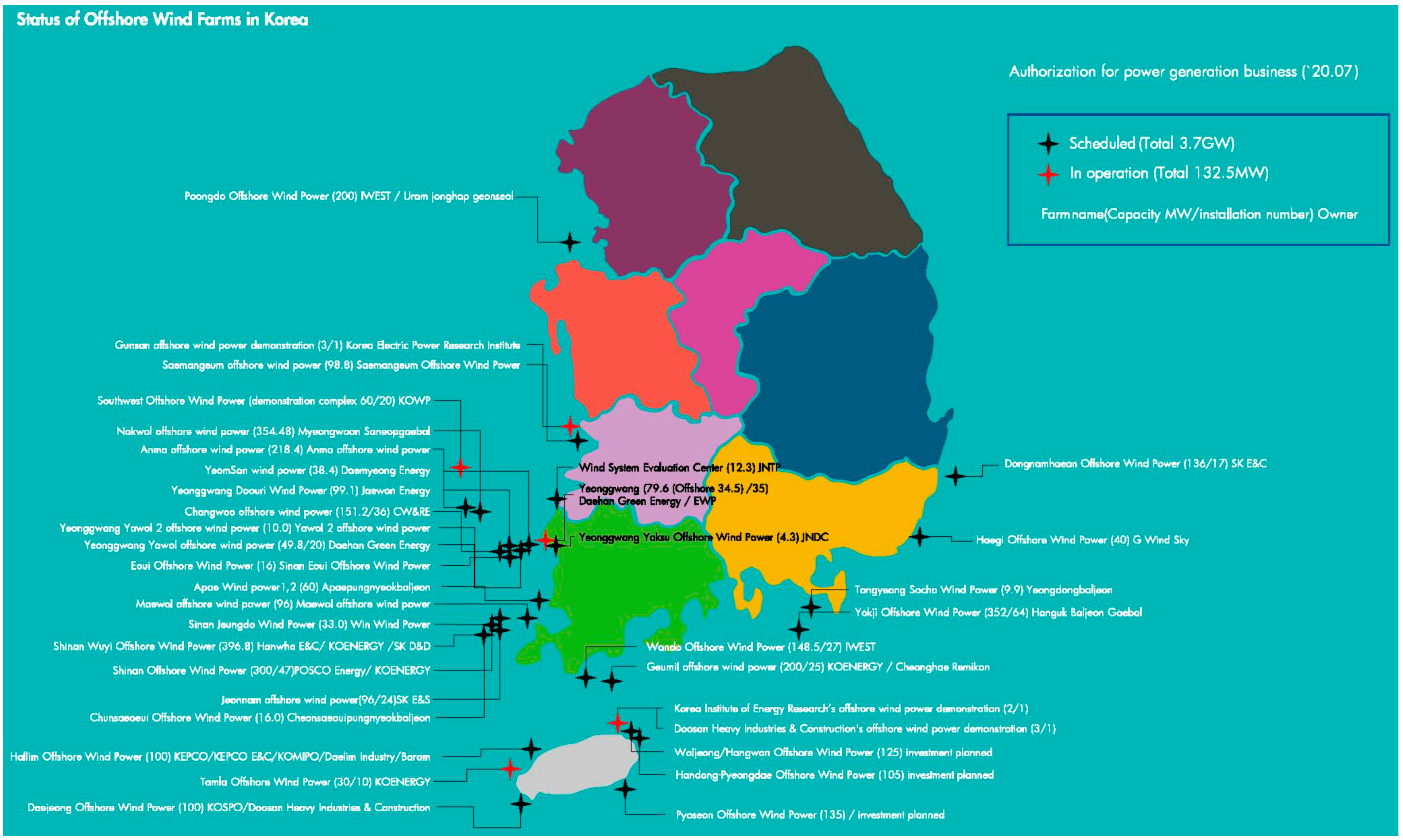
Wind power is now widely used as a renewable, clean, and ecological resource that is qualified to lead the energy transition process [1]. At the end of 2019, wind power generation of 60 GW was newly installed (54 GW on land and 6.1 GW on sea), and the total cumulative capacity reached 651 GW. According to the Global Wind Energy Council (GWEC), the cumulative amount of offshore wind power generation installed around the world in 2019 was 29.1 GW, and with the increase of offshore wind power complexes, offshore wind power generation is a rapidly growing industry in global electricity production [2]. Many governments and countries have implemented a huge number of renewable consolidation policies. As of June 2020, Korea has five offshore wind power projects totaling 132.5 MW, including a 60 MW southwest sea wind pilot project completed in January as the first phase of a large-scale 2.5 GW project. More than 23 offshore wind power projects totaling 7.3 GW are under preliminary development, as shown in Figure 1 [2]. The main purpose of a wind farm operator is to manage the operation of a wind farm system as a whole and determine the optimal set point of the wind turbine generators (WTGs) to achieve different operational objectives. A collective operational objective in a wind farm system is to maximize the output power of the entire system [3]. As part of efforts to maximize efficiency and energy production and to reduce installation costs, proper quantities of wind power plants and their deployment remain important issues to be further investigated [4]. Further developments have been made in recent years to optimize wind turbines in larger wind farms [5].
Ramos et al. [6] analyzed the factors that affect wind farm energy production and indicated that the location selection of a wind farm is very important. Grady et al. [7] applied a genetic algorithm to determine the optimal placement of wind turbines, maximize production capacity, and limit the number of turbines and land acreage in wind power plants. Marmidis et al. [8] used the Monte Carlo procedure to extract the optimum number and placement of wind turbines. Lazarou et al. [9] used the Powell optimization method and Ekonomou et al. [10] used artificial neural networks to determine the optimum number of wind turbines and total production power. Yang et al. [11] proposed a new wind farm layout optimization model to maximize the equivalent power of a wind farm system using the particle swarm optimization algorithm. Feng et al. [12] presented a random search algorithm based on continuous formulation for wind farm layout optimization to provide greater power generation. Gionfra et al. [13] presented a distributed approach to the problem of wind farm power maximization, taking into account the wake interaction among WTGs as a distributed particle cluster optimization algorithm. The influence of turbulence intensity from wind turbine wake in wind farm systems was also investigated in [14]. For the accuracy of an annual energy production forecast in a wind farm, the wind speed reduction due to the wake effects of each wind direction and the accompanying loss of generation should be calculated.
Therefore, the installation layout of a wind turbine plays an important role in the design of every wind farm. In this study, we developed a design support Excel automation program and wind turbine optimal layout design formula to maximize production energy by minimizing energy loss due to the wake within a limited space when designing a wind farm.
2. Offshore Site and Data
2.1. Wind Climate
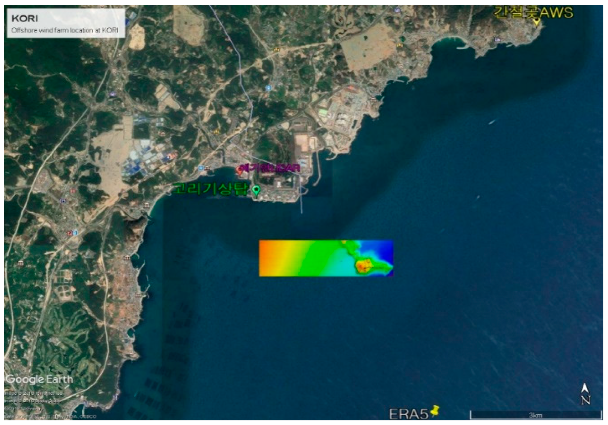
Each wind power plant project begins with the evaluation and selection of the optimal location. The wind speed factor is considered the most relevant parameter for annual energy production, accounting for over 90% of contributions [1]. Figure 2 is a satellite photo of a candidate site for the offshore wind farm located the coast of Kori, located in the southeast of the Korean Peninsula. The location of the ground-based Wind Lidar, the location of the met mast used for long-term wind correction, and the location of the Kanjeolgot automated weather station (AWS), which is the Korea Meteorological Administration’s AWS for verification, are also marked with the water depth measurement results.
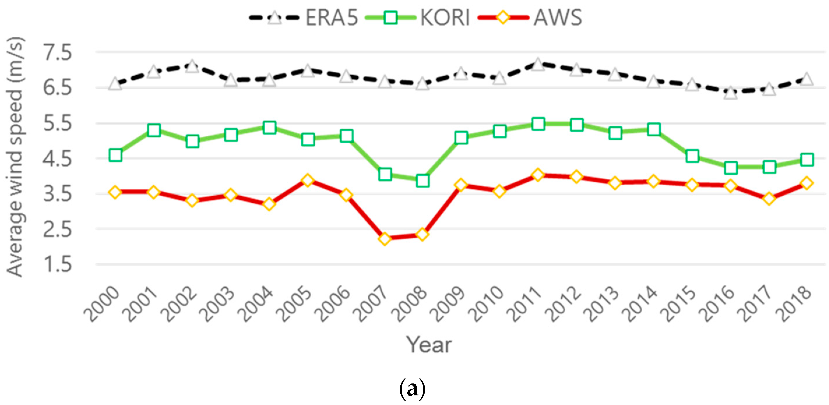
Figure 3 shows a comparison of the long-term average wind speeds from the annular met mast and the long-term ERA5 numerical model. The ERA5 numerical model is based on a maritime location about 7 km from the annular tower. The met mast gives the measured wind speed at 58 m above the ground, while the Kanjeolgot AWS gives the wind speed measured at a 24 m height. Long-term data of 20 years were used for a comparative analysis of the monthly wind velocity.
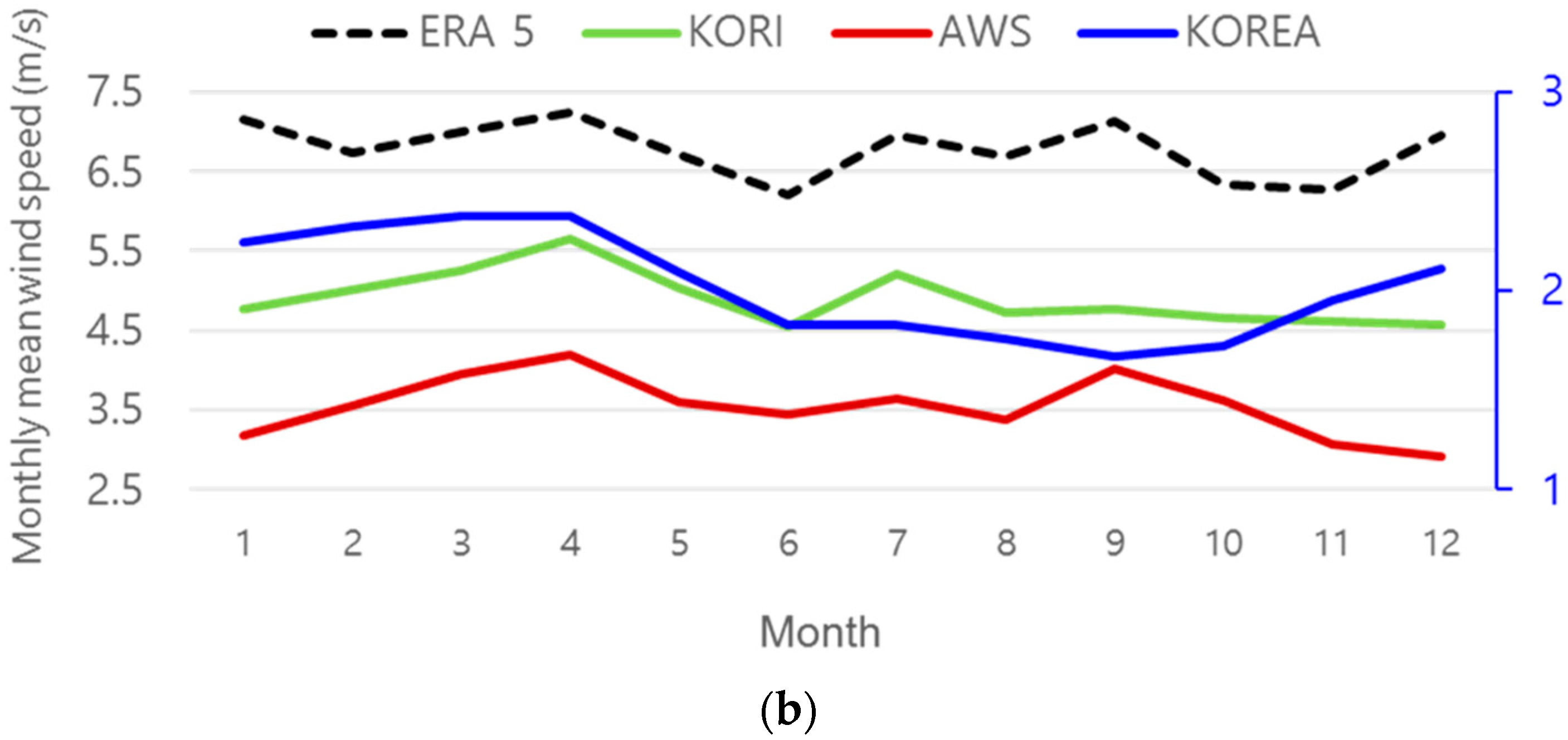
The blue line in Figure 3b represents the average monthly wind speed for Korea over the same 20 years as measured by the Korea Meteorological Administration. Korea’s average seasonal wind speed is generally high in the winter and spring seasons and low in summer and fall. However, unlike typical Korean weather conditions, the average monthly wind speed of the Kori met mast over these 20 years was the lowest during the winter season, and the average wind speed during the spring and fall seasons was observed to be high. Data from the nearby Kanjeolgot AWS also showed similar measurement results, enabling the verification of wind characteristics in the area.
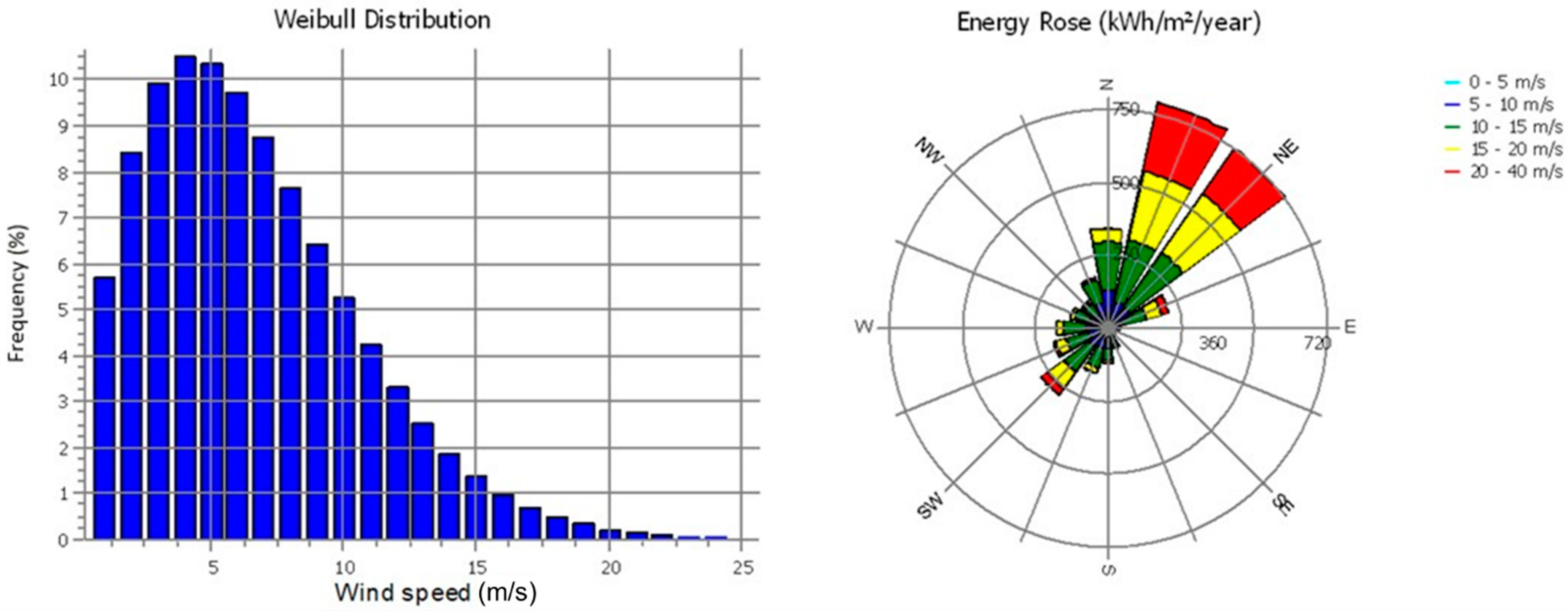
Figure 4 shows the density of wind energy in the area of the intended site of the offshore wind farm using long-term wind speed correction (measure-correlative-predict; MCP) based on the long-term Kori met mast wind data. For a hub height of 110 m, the Weibull parameters (A: scale parameter and K: shape parameter) and the frequency and average wind speed for each direction are summarized, where the main wind direction was NNE. The Weibull distribution parameters were A = 7.14; K = 1.838; and V (mean) = 6.3 m/s.
The windPRO software used in this paper is used by developers, planners, manufacturers, and consultants around the world to design wind power plant layouts and calculate wind power plant production and environmental impact. The turbulence intensity is actually calculated based on the assumption of homogeneous terrain with a surface roughness equal to the roughness length. Input to the calculation is also the turbulence measurement height. The windPRO Software assumes that Ax = 2.5. If a terrain classification exceeded the limits in Table 1 (either the offshore or the open farmland), then the nearest tabular value was chosen [15,16,17].
2.2. Wind Turbine Generator
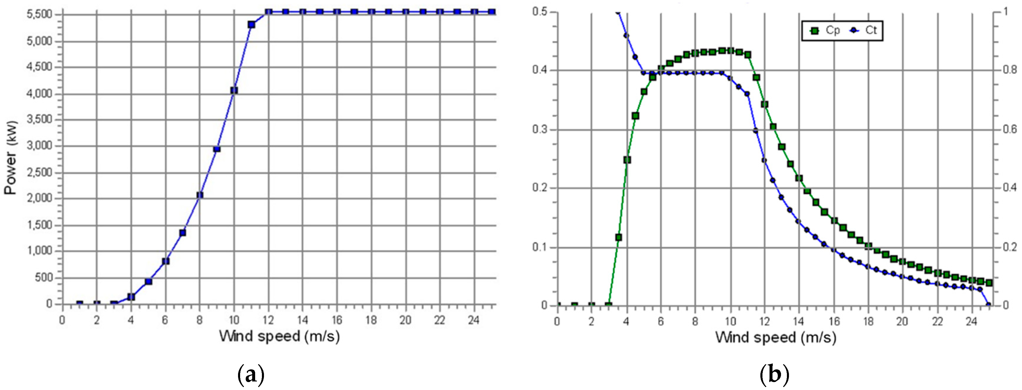
There are two major wind turbine manufacturers in Korea: Doosan Heavy Industries (DHI) and Construction and Hyosung Heavy Industries (HHI). This paper used a commercial offshore wind turbine of DHI. DHI WinDS5500 is more efficient for the areas of strong wind and is specialized in offshore. It was decided to be more accurate to use the wind turbine power curve for the wind turbine power generation at a given wind velocity. The power characteristics of the DHI WinDS5500 turbine are shown in Figure 5, and Table 2 lists the turbine specifications [18]. The range of incoming wind speed was varied between the turbine cut-in speed and cut-out speed.
3. Wind Turbine Layout Automation
3.1. Constraints on Wind Farm Layout
The pilot production amount and size of the Kori offshore wind farm site were 60 MW and 3 × 1 km, respectively, and the wind power generator applied to the turbine placements was made by Doosan Heavy Industries and Construction Co., Ltd. in Korea. The main constraints are summarized as follows:
- (1)
- The assumed wind-power-producing area was placed within a 3 × 1 km square shape. This assumption was useful for proving the ground research data’s effectiveness.
- (2)
- We used actual measured wind conditions as wind.
- (3)
- The turbine layout for industrial wind power areas did not consider additional practical constraints such as dynamic load, shape of the site, and cost of the model.
- (4)
- The wind turbines have identical hub heights and performance.
In this paper, windPRO V3.2, a commercial program developed by EMD International A/S, was used for the calculation and design of the annual power generation of wind farms [19]. Wind farm efficiency is a function of many variables, including atmospheric conditions, terrain, turbine capacity, best turbine solution spacing, and electrical transmission. Generally, it is advantageous in terms of energy production to place the plant site at right angles to the main wind direction, but wind energy is proportional to the cube of wind speed fluctuations and size, so systematic design procedures are required to determine the shape and location of a plant.
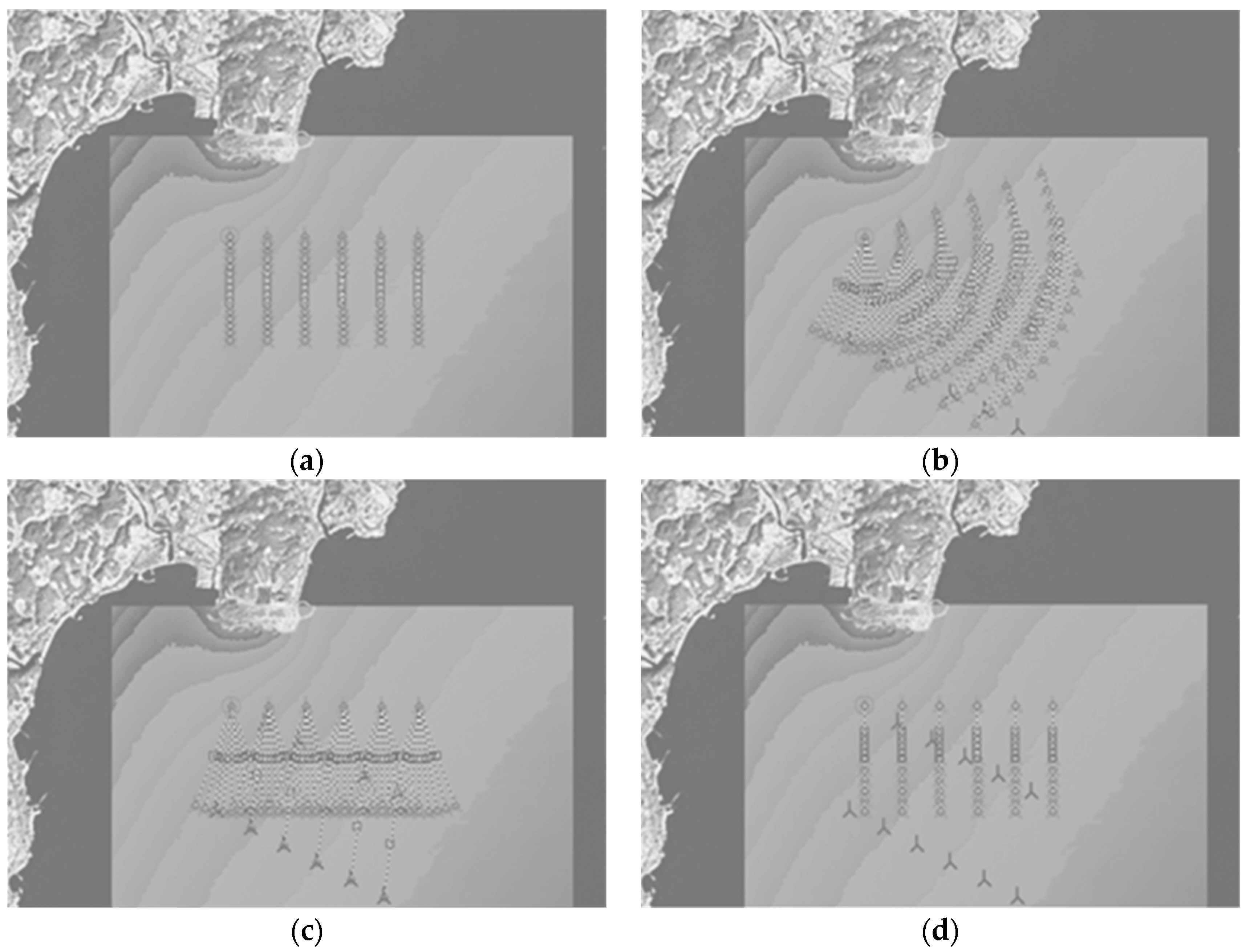
Figure 6 is an example of the deployment of the Kori offshore wind farm turbines using windPRO. The main variables affecting the wind turbine layout were decided to be (a) separation from the shoreline, (b) the rotation angle of the windfarm, (c) the side angle of the windfarm, and (d) the front and rear column distance of the wind turbine generator.
The problem of turbine placement in actual wind farms in Korea is solved by carrying out a turbine layout that is dependent on parameter research or designer judgment through commercial software and the trial-and-error method. Technology accumulation and experience such as a layout algorithm suitable for a domestic power generation environment and the optimization of the turbine layout of an automation concept necessary for farm design are notably lacking compared to advanced countries.
3.2. Defining the Design Variable and Objective Function
The purpose of the wind farm layout optimization problem considered in this paper was to maximize the annual energy production (AEP) for the predefined size and number of turbines of the Kori offshore wind farm and to minimize the wake loss. The issue of optimizing the layout of wind farms for design variables xi according to the two scenarios was formulated as follows.
Find xi = [x1, x2, x3, x4, x5, x6, x7, x8, x9]
Maximize AEP(xi)
Minimize Wake Loss(xi)
Subject to xLower ≤ xi ≤ xUpper i = 1, 2,···, 9
Maximize AEP(xi)
Minimize Wake Loss(xi)
Subject to xLower ≤ xi ≤ xUpper i = 1, 2,···, 9
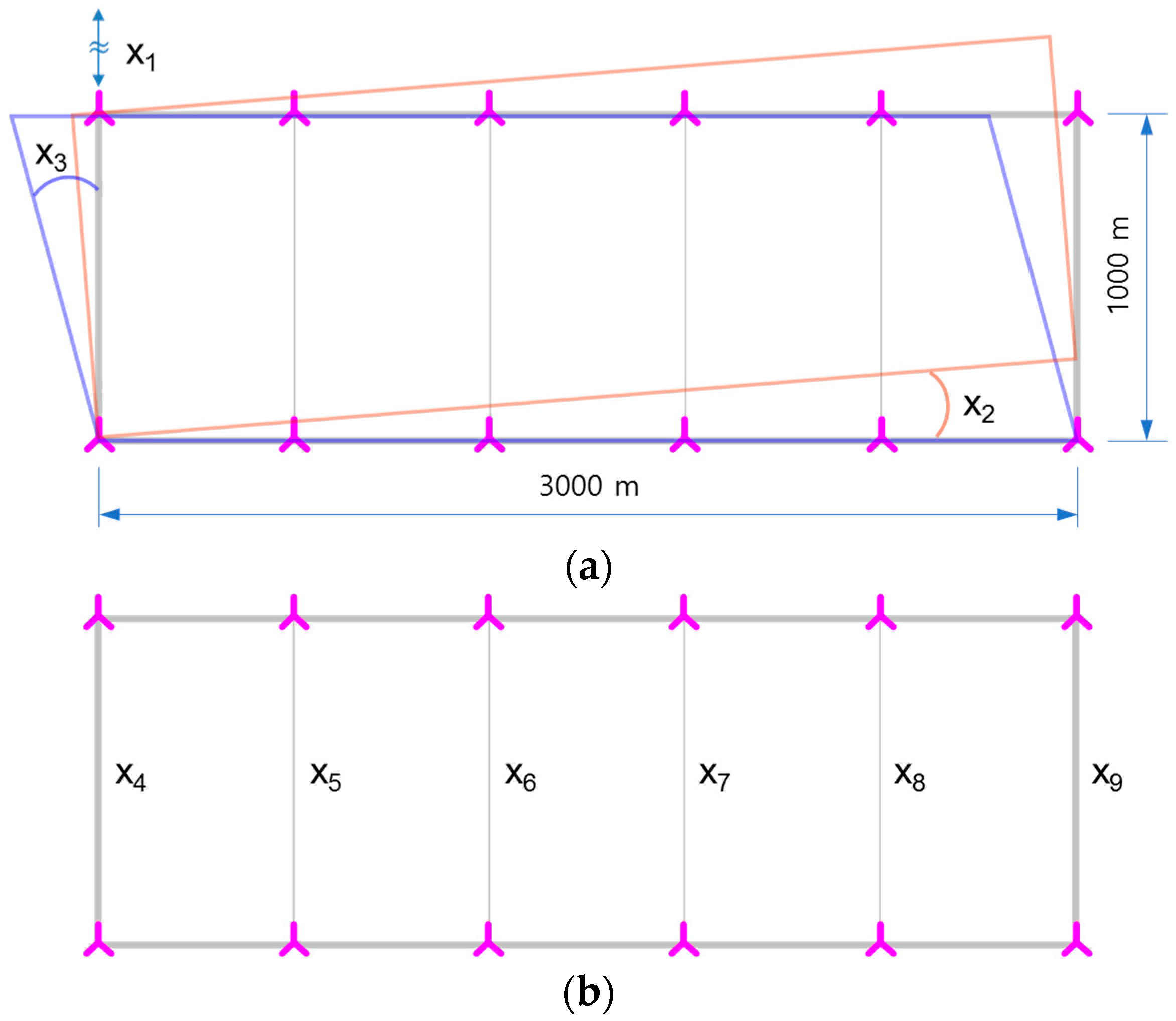
For Scenario 1, Figure 7 represents nine design variables for optimizing the wind farm layout. Coastline separation distance, rotation angle in the main wind direction only, lateral angle only, and separation distance in the front and rear columns of the turbine were selected. Table 3 presents the design variables and their respective levels. Table 4 shows the experimental arrangement and its interpretation results using a Taguchi mixed orthogonal array regarding the nine design variables [20,21].
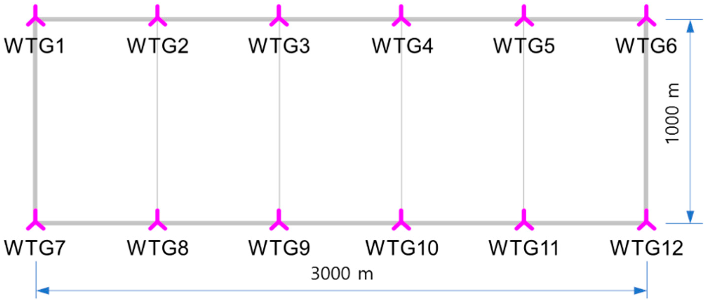
For Scenario 2, Figure 8 defines the 24 x and y coordinates of each turbine as design variables for 12 turbines. In Scenario 2, the turbine placement design of experiment (DOE) sampling implementation program, as a variable, was configured using Visual Studio 2013 C# in Windows 10. The program is run by entering the turbine interval, site size, number of turbines, output file name, and sampling method in the command window. The results of the program execution are checked in the .csv file that is displayed in Excel. The DOE sampling source code for Scenario 2 is shown below.
| DOE (design of experiment) sampling source code for wind farm layout of Scenario 2 |
| class Program { static void writeDataFile(string fileName, DATA[ ] writeData) { StreamWriter objWriter = new StreamWriter(fileName); objWriter.Write(“index, x, y”); //objWriter.WriteLine(“index, x, y”); objWriter.WriteLine(); for (int i = 0; i < writeData.Length; i++) { objWriter.Write(writeData[i].index + “,”); objWriter.Write(writeData[i].x + “,”); objWriter.Write(writeData[i].y + “,”); objWriter.WriteLine(“ “); } objWriter.Close(); } static bool checkValue(DATA[ ] data, double x_val, double y_val, double criteria1) { bool check_value = true; for (int i = 0; i < data.Length; i++) { double delta_x = data[i].x - x_val; double delta_y = data[i].y - y_val; // double radius = Math.Sqrt(delta_x * delta_x + delta_y * delta_y); if (radius < criteria1) { check_value = false; } } // return check_value; } static void Main(string[ ] args) { if (args.Length != 7) { Console.WriteLine(“Argument must be 6 length!!!”); Console.WriteLine(“Current argument is {0}”, (int)args.Length-1); // exit Environment.Exit(-1); |
The interval for the x and y coordinates of the two accumulated turbines were set to at least four times the turbine diameter (4 D) and defined using the following expression [22].
where xij and yij are the arrays storing the wind turbine row and column numbers for the wind turbine x and y coordinates for the unrestricted coordinate method, respectively. The sum of the distances of all pairs i and j is a design constraint to minimize the total distance of the accumulated 12 turbine positions.
3.3. Development of the Metamodel for Wind Turbine Layout
After calculating the amounts of power generated in accordance with Scenarios 1 and 2, the next step was to select an approximation function to use as a turbine-positioning metamodel. We evaluated approximate quality and selected an optimum model for offshore wind farm layout optimization using the polynomials, moving least squares (MLS), kriging interpolation model, and feedforward network methods.
The evaluation of the metamodel quality was performed using the coefficient of determination (CoD) and the coefficient of prognosis (CoP). The degree of agreement between the DOE data and the estimate of the meta-model was measured by the CoP value in Equation (3) for the use of additional test design points [23].
where y is the test value, ŷ is the estimate of the metamodel, and μ and σ are the mean and standard deviation, respectively, calculated from each of the N-many DOE data y(k).
The CoP is calculated in a similar manner as the more common CoD or R2 values, except that it is calculated through a cross-validation process where the data are partitioned into subsets that are each used only for the metamodel calculation or the CoP calculation, not both. For this reason, it is preferred as a measure for how effective the model is at predicting unknown data points, which is particularly valuable in this kind of metamodel application.
Table 5 and Table 6 show the accuracy results of each type of metamodel for wind farm design for two scenarios. The metamodeling techniques considered within the scope of this study included polynomials, MLS, kriging and feedforward network methods. The feedforward network is a deep learning-based metamodel. It uses the Keras library with TensorFlow as backend to create a metamodel by training a neural network [24,25,26]. The accuracy of the metamodels was evaluated by the CoD and the CoP. Scenario 1 was found to have a higher metamodel accuracy than Scenario 2. The metamodel for optimum turbine layout design was the feedforward network with high predictive quality. For example, the AEP had an approximate quality of about 97% and a prediction accuracy of about 96% when compared to the windPRO analysis results at any design point.
ANOVA was used to quantitatively investigate the effects of the design variables on the AEP and wake loss. The results of an ANOVA for the AEP and wake loss are shown in Table 7 and Table 8. Here, the ANOVA was evaluated via the orthogonal analysis of the sensitivity of each variable to the response with a polynomial component. The primary and secondary components in the table are the fractional orders of the design variables and are expressed as F-values. In this paper, we used the F-value to calculate the p-value, which was used to make a decision about the statistical significance of the test. The p-value is a probability that measures the evidence against the null hypothesis. Lower probabilities provide stronger evidence against the null hypothesis. A sufficiently large F-value indicates statistical significance. Therefore, the p-value is a very useful parameter that determines the significance of a design variable.
The percentage contribution by each design variable in the total sum of the squared deviations could be used to evaluate the importance of the design variables’ change on the wind farm layout. The design variables that were found to have a dominant influence on the AEP were the rotation of farm side angle (x3) and the distance between coastlines (x1) in the main wind direction. The effect of the farm side angle (x3) for wake loss was relatively smaller than that of the AEP. The interaction of farm based angle (x2) and farm side angle (x3) existed but was mild.
Equations (4)–(6) were used to indicate an approximate model of the AEP, wake loss, and capacity factor for the wind farm layout by selecting a significant order of the design variables and considering the interaction.
AEP =
148,220 + 17.376 × (x1) − 0.005758 × (x1)2 − 271.69 × (x2)-2.3571 × (x2)2
− 47.64 × (x3) + 0.1139 × (x3)2 + 2.737 × (x4) − 0.000852 × (x4)2 + 2.185 × (x5)
− 0.000320 × (x5)2 + 1.103 × (x6) + 0.000437 × (x6)2 + 3.856 × (x7) − 0.001398
× (x7)2 + 4.832 × (x8) − 0.001909 × (x8)2 + 3.168 × (x9) − 0.000689 × (x9)2
+ 1.4767 × (x2) × (x3)
Wake Loss =
16.7652 − 0.00446667 × (x1) + 0.0272222 × (x2) − 0.0152778 × (x3)
− 0.00142722 × (x4) − 0.00107619 × (x5) + 0.00155448 × (x6) − 0.00195342
× (x7) − 0.00227908 × (x8) − 0.00195308 × (x9) + 1.77778 × 10⁶ × (x12)
+ 0.00111111 × (x22) + 6.94444 × 10⁵ × (x32) + 3.94539 × 10⁷ × (x42) + 5.63627
× 108 × (x52) − 1.46543 × 10⁶ × (x62) + 7.32715 × 10⁷ × (x72) + 9.01803 × 10⁷
× (x82) + 5.63627 × 10⁷ × (x92)
Capacity Factor =
24.4237 + 0.000355556 × (x1) − 0.0216667 × (x2) − 0.00375 × (x3)
+ 0.000262763 × (x4) + 0.000325325 × (x5) + 0.000237738 × (x6)
+ 0.000262763 × (x7) + 0.0003003 × (x8) + 0.000337838 × (x9)
24.4237 + 0.000355556 × (x1) − 0.0216667 × (x2) − 0.00375 × (x3)
+ 0.000262763 × (x4) + 0.000325325 × (x5) + 0.000237738 × (x6)
+ 0.000262763 × (x7) + 0.0003003 × (x8) + 0.000337838 × (x9)
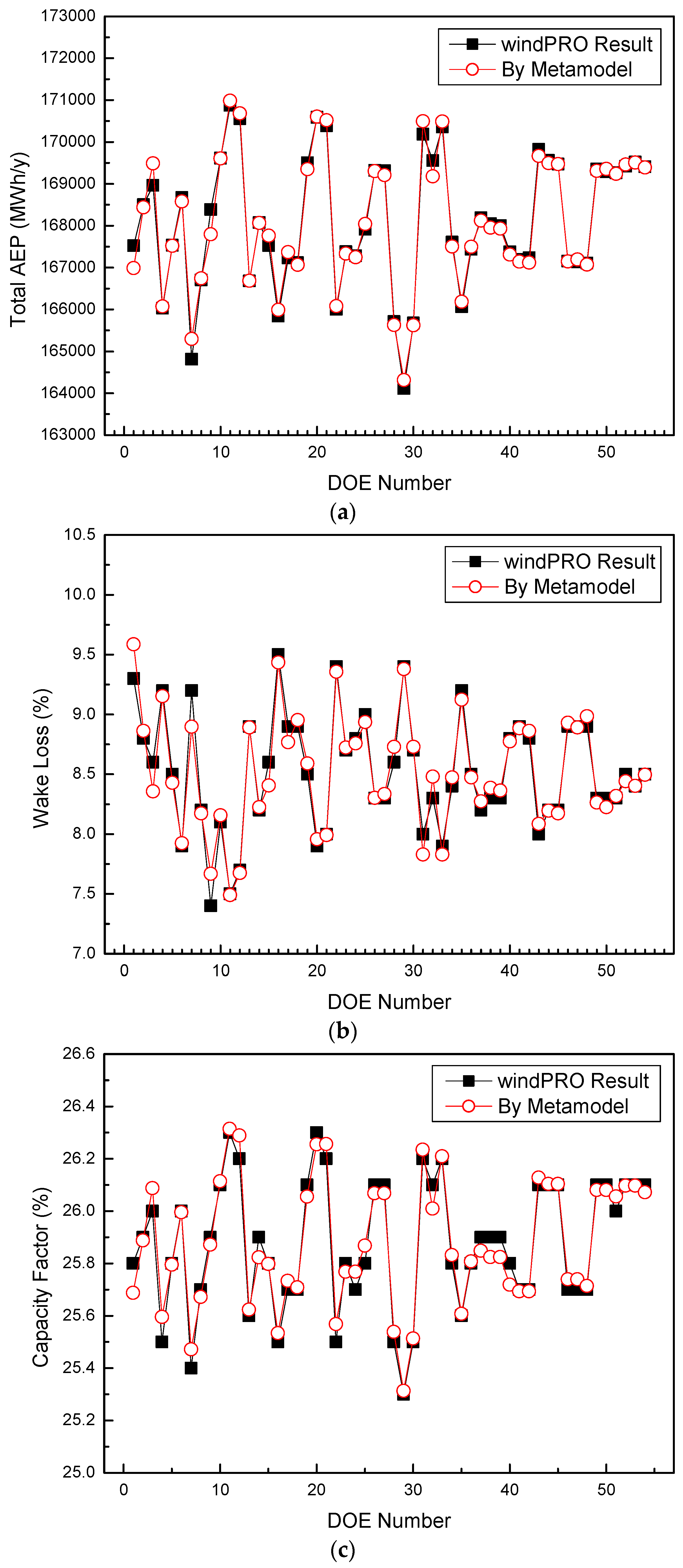
Figure 9 compares the polynomial-based metamodel in Equations (4)–(6) and the windPRO analysis result of the AEP, wake loss, and capacity factor, respectively. The total errors between the metamodel and the windPRO analysis, i.e., R2 for the AEP, wake loss, and capacity factor, were 98.7%, 95.9%, and 97.6%, respectively; the R2 adjusted values were 97.9%, 93.5%, and 96.2%, respectively. Hence, the accuracies of the metamodels were considered adequate for this paper. It can be seen that the approximation values agreed well with the windPRO analysis result on the whole.
3.4. Design Support Excel Automation Program
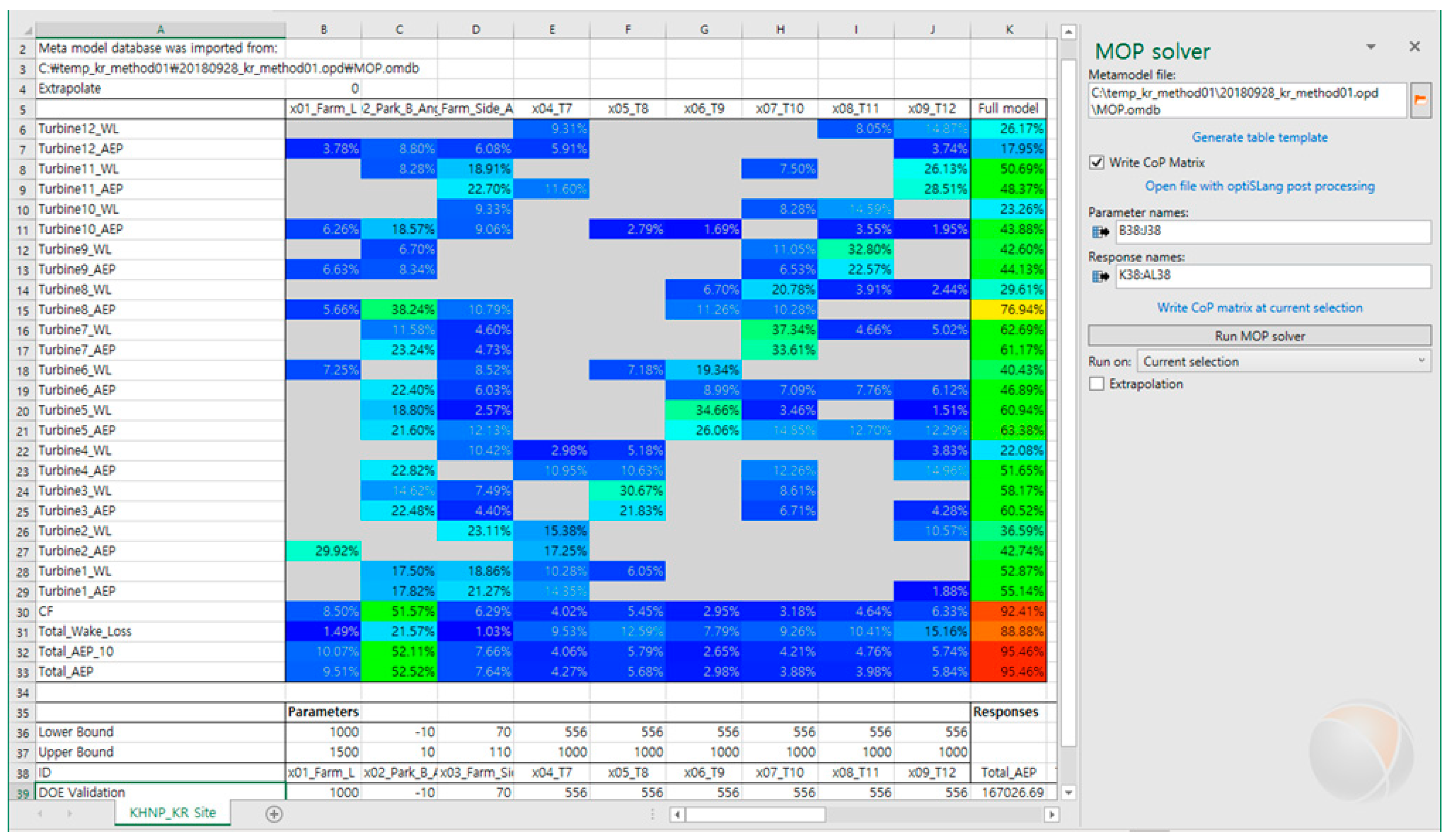
Figure 10 shows the Excel metamodel solver for turbine layout calculation using optiSLang and Python script. A metamodel solver (also called Metamodel of Optimal Prognosis (MOP) Solver) and a CoP Matrix for optimal turbine placement were created for use in Excel. The two main features were as follows.
CoP Matrix: The full model CoPs for every output parameter were shown in the last column in Excel automation program display. The single CoP values of the input parameters were shown line-by-line. When using the CoP matrix, the most important input parameters could be determined and the forecast qualities of the identified surrogate models could be evaluated.
MOP Solver: The MOP Solver was integrated in Excel to use metamodels for windPRO calculations. Starting from a reduced number of simulations, a metamodel (polynomial or feedforward network) of the original physical problem could be used to perform various possible design configurations for a wind farm layout without computing any further analyses. The metamodel results were stored in an optiSLang monitoring database file and could be used for the MOP Solver calls to replace the original solver process.
The AEP, wake loss, and utilization rates of 12 individual turbines and the entire wind farm were obtained in real time in seconds without windPRO calculations for arbitrary positions of wind turbines. In addition to the arrangement of turbines, wind farms also need to define parameters for various design conditions (ground area, installation cost, fatigue, etc.). Whenever the parameters for these design conditions are modified, design re-evaluation is time-consuming and costly. Therefore, linking approximation models for different design conditions on the basis of a proven metamodel for turbine deployment is expected to provide insight to select and compromise on various turbine deployments and design conditions.
4. Conclusions and Future Work
An Excel metamodel solver for turbine layout calculation using Python script was created in this work. The AEP, wake loss, and utilization rates of each of the 12 individual turbines and an entire wind farm were obtained within seconds without windPRO calculations for the turbines’ arbitrary design points. The automated turbine placement calculations using metamodels helped to understand the AEP and wake loss for turbine layout, thus allowing for cost models, turbine life assessments for digital twins, and other extensions to this task. Additionally, using our approach, plant designers could save significant money and time that could be spent calculating wind farm layouts. Since our demonstration is a small area, the savings could actually be even greater if considering a larger offshore site for a new project.
Author Contributions
Conceptualization, J.S.; data curation, J.S.; formal analysis, S.B.; investigation, J.S.; methodology, S.B. and Y.R.; software, J.S. and S.B.; supervision, Y.R.; validation, Y.R.; writing—original draft, J.S. and S.B.; writing—review and editing, J.S., S.B., and Y.R. All authors have read and agreed to the published version of the manuscript.
Funding
This work was supported by the Korea Institute of Energy Technology Evaluation and Planning (KETEP) and the Ministry of Trade, Industry and Energy (MOTIE) of the Republic of Korea (No. 20163010024750).
Conflicts of Interest
The authors declare no conflict of interest.
References
- Gil-García, I.C.; García-Cascales, M.S.; Fernández-Guillamón, A.; Molina-García, A. Categorization and analysis of relevant factors for optimal locations in onshore and offshore wind power plants: A taxonomic review. J. Mar. Sci. Eng. 2019, 7, 391. [Google Scholar] [CrossRef] [Green Version]
- Global Wind Energy Council (GWEC). Global Offshore Wind Report 2020; GWEC: Brussels, Belgium, 2020; Volume 19, pp. 10–12, 63–65. [Google Scholar]
- Bui, V.-H.; Hussain, A.; Lee, W.-G.; Kim, H.-M. Multi-objective optimization for determining trade-off between output power and power fluctuations in wind farm system. Energies 2019, 12, 4242. [Google Scholar] [CrossRef] [Green Version]
- Christodoulou, C.A.; Vita, V.; Seritan, G.-C.; Ekonomou, L. A harmony search method for the estimation of the optimum number of wind turbines in a wind farm. Energies 2020, 13, 2777. [Google Scholar] [CrossRef]
- Al-Addous, M.; Jaradat, M.; Wellmann, A.A.J.; Al Hmidan, S. The significance of wind turbines layout optimization on the predicted farm energy yield. Atmosphere 2020, 11, 117. [Google Scholar] [CrossRef] [Green Version]
- Ramos, C.A.; Ramirez, D.; Jin, K.; Li, H. Factorial analysis of selected factors affecting the electricity production of onshore wind farms. Int. J. Energy Clean. Environ. 2011, 12, 67–77. [Google Scholar] [CrossRef]
- Grady, S.A.; Hussaini, M.Y.; Abdullah, M.M. Placement of wind turbines using genetic algorithms. Renew. Energy 2005, 30, 259–270. [Google Scholar] [CrossRef]
- Marmidis, G.; Lazarou, S.; Pyrgioti, E. Optimal placement of wind turbines in a wind park using Monte Carlo simulation. Renew. Energy 2008, 33, 1455–1460. [Google Scholar] [CrossRef]
- Lazarou, S.; Vita, V.; Ekonomou, L. Application of Powell’s optimization method for the optimal number of wind turbines in a wind farm. IET Sci. Meas. Technol. 2011, 5, 77–80. [Google Scholar] [CrossRef]
- Ekonomou, L.; Lazarou, S.; Chatzarakis, G.E.; Vita, V. Estimation of wind turbines optimal number and produced power in a wind farm using an artificial neural network model. Simul. Model. Pract. Theory 2012, 21, 21–25. [Google Scholar] [CrossRef]
- Yang, H.; Xie, K.; Tai, H.M.; Chai, Y. Wind farm layout optimization and its application to power system reliability analysis. IEEE Trans. Power Syst. 2015, 31, 2135–2143. [Google Scholar] [CrossRef]
- Feng, J.; Shen, W.Z. Solving the wind farm layout optimization problem using random search algorithm. Renew. Energy 2015, 78, 182–192. [Google Scholar] [CrossRef]
- Gionfra, N.; Sandou, G.; Siguerdidjane, H.; Faille, D.; Loevenbruck, P. Wind farm distributed PSO-based control for constrained power generation maximization. Renew. Energy 2019, 133, 103–117. [Google Scholar] [CrossRef]
- Hansen, K.S.; Barthelmie, R.J.; Jensen, L.E.; Sommer, A. The impact of turbulence intensity and atmospheric stability on power deficits due to wind turbine wakes at Horns Rev wind farm. Wind Energy 2012, 15, 183–196. [Google Scholar] [CrossRef] [Green Version]
- Andersen, P.S.; Krabbe, U.; Lundsager, P.; Petersen, H. Basismateriale for Beregning af Propelvindmøller; Risø-M-2153 (rev.); Forsøgsanlæg Risø: Roskilde, Denmark, 1980. [Google Scholar]
- Schepers, J.G. ENDOW: Validation and Improvement of ECN’s Wake Model; ECN-C-03-037; Energy Research Centre of the Netherlands ECN: Petten, The Netherlands, 2003. [Google Scholar]
- Risø National Laboratory. Guidelines for Design of Wind Turbines, DNV/Risø, 2nd ed.; Risø National Laboratory: Roskilde, Denmark, 2002. [Google Scholar]
- Available online: http://www.doosanheavy.com/download/pdf/products/energy/DHI_Wind_Power_Brochure_Eng.pdf (accessed on 1 December 2020).
- EMD International A/S. Introduction to wind turbine wake modeling and wake generated turbulence. In WindPRO/PARK; EMD International A/S: Aalborg, Denmark, 2019. [Google Scholar]
- Phadke, M. Quality Engineering Using Robust Design; Prentice Hall: Englewood Cliffs, NJ, USA, 1989. [Google Scholar]
- Florian, A. An efficient sampling scheme: Latin hypercube sampling. Probabilistic Eng. Mech. 1992, 279, 123–130. [Google Scholar] [CrossRef]
- Shin, J.; Baek, S.; Rhee, Y. Wind Farm Layout Optimization Using a Metamodel And Ea/Pso Algorithm In Korea Offshore. Energies 2021, 14, 146. [Google Scholar] [CrossRef]
- Dynardo GmbH. OptiSlang; Version 7.5.1; Documentation; Dynardo GmbH: Weimar, Germany, 2019. [Google Scholar]
- Simpson, T.W.; Peplinski, J.; Koch, P.N.; Allen, J.K. Metamodels for computer-based engineering design: Survey and recommendations. Eng. Comput. 2001, 17, 129–150. [Google Scholar] [CrossRef] [Green Version]
- Roos, D.; Most, T.; Unger, J.F.; Will, J. Advanced surrogate models within the robustness evaluation. In Proceedings of the Weimarer Optimierungs-und Stochastiktage 4.0, Weimar, Germany, 29–30 November 2007. [Google Scholar]
- Dynardo GmbH. optiSLang DLE (Deep Learning Extension); Dynardo GmbH: Weimar, Germany, 2019. [Google Scholar]
Figure 1.
Offshore wind farm locations in Korea (source: Korea Energy Industry Association).

Figure 2.
Offshore wind farm location at Kori.

Figure 3.
Average wind speed in Kori offshore over 20-year period: (a) Annual mean wind speed and (b) monthly mean wind speed.
Figure 3.
Average wind speed in Kori offshore over 20-year period: (a) Annual mean wind speed and (b) monthly mean wind speed.


Figure 4.
Wind rose diagram at Kori.

Figure 5.
The power characteristics of Doosan Heavy Industries (DHI) WinDS5500 turbine: (a) DHI WinDS5500 power curve and (b) DHI WinDS5500 thrust coefficient curve.
Figure 5.
The power characteristics of Doosan Heavy Industries (DHI) WinDS5500 turbine: (a) DHI WinDS5500 power curve and (b) DHI WinDS5500 thrust coefficient curve.

Figure 6.
Basic pattern of wind turbine layout at the Kori offshore wind farm: (a) Coastline distance, (b) base angle, (c) side angle, and (d) column distance.
Figure 6.
Basic pattern of wind turbine layout at the Kori offshore wind farm: (a) Coastline distance, (b) base angle, (c) side angle, and (d) column distance.

Figure 7.
Design variables for the offshore wind farm layout based on a regular pattern (Scenario 1): (a) Farm pattern and (b) wind turbine generator (WTG) column distance.
Figure 7.
Design variables for the offshore wind farm layout based on a regular pattern (Scenario 1): (a) Farm pattern and (b) wind turbine generator (WTG) column distance.

Figure 8.
Design variables for the offshore wind farm layout based on unrestricted coordinates (Scenario 2).
Figure 8.
Design variables for the offshore wind farm layout based on unrestricted coordinates (Scenario 2).

Figure 9.
Comparison between windPRO result and metamodel in design of experiment (DOE) number: (a) Total AEP, (b) wake loss, and (c) capacitor factor.
Figure 9.
Comparison between windPRO result and metamodel in design of experiment (DOE) number: (a) Total AEP, (b) wake loss, and (c) capacitor factor.

Figure 10.
The design support Excel automation program display for wind farm layout optimization.


Table 1.
Typical wake model parameters.
| Terrain Classification | Roughness Class | Roughness Length | Wake Decay Constant | Ambient Turbulence at 50 m Ax = 1.8 | Ambient Turbulence at 50 m Ax = 2.5 | Additional Detailed Description |
|---|---|---|---|---|---|---|
| Offshore water areas | 0.0 | 0.0002 | 0.040 | 0.06 | 0.08 | Oceans and large lakes. General water bodies |
| Mixed water and land | 0.5 | 0.0024 | 0.052 | 0.07 | 0.10 | Mixed water and land |
| Very open farmland | 1.0 | 0.0300 | 0.063 | 0.10 | 0.13 | No cross hedges. Scattered buildings |
| Open farmland | 1.5 | 0.0500 | 0.075 | 0.11 | 0.15 | Some buildings. Crossing hedges with an 8 m height with a distance of 1250 m apart |
Table 2.
WindDS5500 system specification.
| Item | Value | |
|---|---|---|
| Operational Data | Rated Power | 5560 kW |
| Class | IB | |
| Cut-in Wind Speed | 3.5 m/s | |
| Rated Wind Speed | 13 m/s | |
| Cut-out Wind Speed | 25 m/s | |
| Rotor Diameter | 140 m | |
| Extreme Survival Wind Speed | 70 m/s | |
| Blade | Length | 68 m |
| Tower | Hub Height | Site-specific |
Table 3.
Design variables and their levels.
| Design Variable | Description | Unit | Initial | Level 1 | Level 2 | Level 3 |
|---|---|---|---|---|---|---|
| x1 | Coastline Distance | m | 1000 | 1000 | 1250 | 1500 |
| x2 | Farm Base Angle | Degree | 0 | −10 | 0 | 10 |
| x3 | Farm Side Angle | Degree | 90 | 70 | 90 | 110 |
| x4 | 1 × 1 Row Distance | m | 1000 | 556 | 778 | 1000 |
| x5 | 1 × 2 Row Distance | m | 1000 | 556 | 778 | 1000 |
| x6 | 1 × 3 Row Distance | m | 1000 | 556 | 778 | 1000 |
| x7 | 1 × 4 Row Distance | m | 1000 | 556 | 778 | 1000 |
| x8 | 1 × 5 Row Distance | m | 1000 | 556 | 778 | 1000 |
| x9 | 1 × 6 Row Distance | m | 1000 | 556 | 778 | 1000 |
Table 4.
Taguchi orthogonal array L54 matrix and results. AEP: annual energy production; CF: capacity factor.
Table 4.
Taguchi orthogonal array L54 matrix and results. AEP: annual energy production; CF: capacity factor.
| No. | x1 | x2 | x3 | x4 | x5 | x6 | x7 | x8 | x9 | AEP (MWh/y) | Wake Loss (%) | CF (%) |
|---|---|---|---|---|---|---|---|---|---|---|---|---|
| 1 | 1000 | −10 | 70 | 556 | 556 | 556 | 556 | 556 | 556 | 167,518.2 | 9.3 | 25.8 |
| 2 | 1000 | −10 | 70 | 556 | 556 | 556 | 778 | 778 | 778 | 168,502.4 | 8.8 | 25.9 |
| ⋮ | ⋮ | ⋮ | ||||||||||
| 54 | 1500 | 0 | 70 | 778 | 1000 | 556 | 1000 | 778 | 556 | 169,410.6 | 8.5 | 26.1 |
Table 5.
Accuracy of metamodeling techniques for Scenario 1. MLS: moving least squares; CoD: coefficient of determination; CoP: coefficient of prognosis.
Table 5.
Accuracy of metamodeling techniques for Scenario 1. MLS: moving least squares; CoD: coefficient of determination; CoP: coefficient of prognosis.
| Metamodel Type | Response | No. Parameters | No. Coefficients | CoD | CoP |
|---|---|---|---|---|---|
| Polynomial (Box–Cox) | AEP | 9 | 10 | 0.967 | 0.955 |
| Wake Loss | 9 | 19 | 0.932 | 0.889 | |
| Capacity Factor | 9 | 10 | 0.944 | 0.924 | |
| MLS (exponential weight) | AEP | 6 | 7 | 0.864 | 0.839 |
| Wake Loss | 4 | 5 | 0.620 | 0.568 | |
| Capacity Factor | 6 | 7 | 0.836 | 0.807 | |
| Kriging (isotropic kernel) | AEP | 6 | 1 | 0.942 | 0.853 |
| Wake Loss | 6 | 1 | 0.726 | 0.852 | |
| Capacity Factor | 6 | 1 | 0.915 | 0.817 | |
| Feedforward network | AEP | 9 | 9 | 0.996 | 0.979 |
| Wake Loss | 9 | 9 | 0.912 | 0.914 | |
| Capacity Factor | 9 | 9 | 0.988 | 0.962 |
Table 6.
Accuracy of metamodeling techniques for Scenario 2.
| Metamodel Type | Turbine Number | Response | No. Parameters | No. Coefficients | CoD | CoP |
|---|---|---|---|---|---|---|
| Kriging (isotropic kernel) | WTG1 | AEP | 6 | 1 | 0.804 | 0.431 |
| Polynomial (no mixed term) | Wake Loss | 2 | 5 | 0.657 | 0.587 | |
| Polynomial (with mixed terms) | WTG2 | AEP | 2 | 6 | 0.710 | 0.684 |
| Polynomial (with mixed terms) | Wake Loss | 2 | 6 | 0.827 | 0.812 | |
| Polynomial (no mixed term) | WTG3 | AEP | 3 | 7 | 0.703 | 0.674 |
| Polynomial (Box–Cox) | Wake Loss | 3 | 7 | 0.829 | 0.811 | |
| Polynomial (no mixed term) | WTG4 | AEP | 6 | 13 | 0.754 | 0.645 |
| Polynomial (no mixed term) | Wake Loss | 5 | 11 | 0.757 | 0.660 | |
| MLS (exponential weight) | WTG5 | AEP | 2 | 5 | 0.807 | 0.674 |
| MLS (exponential weight) | Wake Loss | 2 | 5 | 0.840 | 0.730 | |
| Kriging (isotropic kernel) | WTG6 | AEP | 2 | 1 | 0.792 | 0.618 |
| Polynomial (Box–Cox) | Wake Loss | 3 | 10 | 0.835 | 0.797 | |
| Kriging (isotropic kernel) | WTG7 | AEP | 4 | 1 | 0.851 | 0.685 |
| Kriging (isotropic kernel) | Wake Loss | 3 | 1 | 0.881 | 0.724 | |
| MLS (exponential weight) | WTG8 | AEP | 2 | 5 | 0.867 | 0.744 |
| MLS (exponential weight) | Wake Loss | 2 | 5 | 0.918 | 0.843 | |
| MLS (exponential weight) | WTG9 | AEP | 5 | 11 | 0.727 | 0.593 |
| Kriging (isotropic kernel) | Wake Loss | 4 | 1 | 0.966 | 0.809 | |
| Polynomial (with mixed terms) | WTG10 | AEP | 2 | 6 | 0.728 | 0.682 |
| Polynomial (with mixed terms) | Wake Loss | 2 | 6 | 0.729 | 0.682 | |
| Kriging (isotropic kernel) | WTG11 | AEP | 3 | 1 | 0.931 | 0.787 |
| Kriging (isotropic kernel) | Wake Loss | 3 | 1 | 0.957 | 0.887 | |
| Polynomial (with mixed terms) | WTG12 | AEP | 2 | 6 | 0.782 | 0.724 |
| Polynomial (with mixed terms) | Wake Loss | 2 | 6 | 0.889 | 0.861 |
Table 7.
Analysis of variance for the AEP.
| Design Variable | Sum of Squares | Degree of Freedom | F-Value | p-Value | Percentage Contribution (%) | |
|---|---|---|---|---|---|---|
| x1 | Linear | 12,848,521 | 1 | 19.56 | 0 | 20.9 |
| Quadratic | 540,417 | 1 | 14.86 | 0 | 0.1 | |
| x2 | Linear | 69,342,815 | 1 | 20.82 | 0 | 15.9 |
| Quadratic | 666,685 | 1 | 12.75 | 0.001 | 0.2 | |
| x3 | Linear | 10,607,289 | 1 | 2.56 | 0.119 | 22.3 |
| Quadratic | 24,901 | 1 | 0.48 | 0.495 | 0.1 | |
| x4 | Linear | 5,394,393 | 1 | 1.45 | 0.237 | 13.6 |
| Quadratic | 12,175 | 1 | 0.32 | 0.573 | 3.6 | |
| x5 | Linear | 7,241,302 | 1 | 0.92 | 0.343 | 2.7 |
| Quadratic | 40,476 | 1 | 0.05 | 0.832 | 1.2 | |
| x6 | Linear | 3,735,458 | 1 | 0.21 | 0.650 | 0.5 |
| Quadratic | 109,201 | 1 | 0.09 | 0.772 | 5.7 | |
| x7 | Linear | 5,010,360 | 1 | 3.40 | 0.074 | 1.6 |
| Quadratic | 56,989 | 1 | 1.09 | 0.304 | 2.2 | |
| x8 | Linear | 6,143,541 | 1 | 5.34 | 0.027 | 0.3 |
| Quadratic | 106,251 | 1 | 2.03 | 0.163 | 2.4 | |
| x9 | Linear | 7,789,495 | 1 | 2.29 | 0.139 | 1.0 |
| Quadratic | 13,849 | 1 | 0.26 | 0.610 | 0.3 | |
| x2 x3 | Interaction | 261,685 | 1 | 5.00 | 0.032 | 5.3 |
| Total | 129,945,804 | 19 | 93.48 | 100 | ||
Table 8.
Analysis of variance for wake loss.
| Design Variable | Sum of Squares | Degree of Freedom | F-Value | p-Value | Percentage Contribution (%) | |
|---|---|---|---|---|---|---|
| x1 | Linear | 0.00111 | 1 | 11.69 | 0.002 | 17.2 |
| Quadratic | 0.14815 | 1 | 11.99 | 0.001 | 1.1 | |
| x2 | Linear | 2.66778 | 1 | 6.72 | 0.014 | 17.6 |
| Quadratic | 0.14815 | 1 | 9.99 | 0.003 | 0.2 | |
| x3 | Linear | 0.11111 | 1 | 0.93 | 0.342 | 9.9 |
| Quadratic | 0.00926 | 1 | 0.62 | 0.435 | 1.6 | |
| x4 | Linear | 1.17361 | 1 | 3.46 | 0.071 | 14.7 |
| Quadratic | 0.00454 | 1 | 1.62 | 0.212 | 4.5 | |
| x5 | Linear | 1.73361 | 1 | 2.47 | 0.125 | 1.4 |
| Quadratic | 0.00009 | 1 | 0.72 | 0.402 | 1.5 | |
| x6 | Linear | 0.93444 | 1 | 0.12 | 0.726 | 0.9 |
| Quadratic | 0.06259 | 1 | 1.12 | 0.297 | 6.2 | |
| x7 | Linear | 1.17361 | 1 | 3.08 | 0.088 | 5.1 |
| Quadratic | 0.01565 | 1 | 1.05 | 0.312 | 2.4 | |
| x8 | Linear | 1.36111 | 1 | 4.19 | 0.049 | 2.4 |
| Quadratic | 0.02370 | 1 | 1.60 | 0.215 | 4.5 | |
| x9 | Linear | 2.05444 | 1 | 3.07 | 0.089 | 3.6 |
| Quadratic | 0.00926 | 1 | 0.62 | 0.435 | 0.9 | |
| x2 x3 | Interaction | 0.04481 | 1 | 3.02 | 0.091 | 4.4 |
| Total | 11.67704 | 19 | 68.08 | 100 | ||
Publisher’s Note: MDPI stays neutral with regard to jurisdictional claims in published maps and institutional affiliations. |
© 2021 by the authors. Licensee MDPI, Basel, Switzerland. This article is an open access article distributed under the terms and conditions of the Creative Commons Attribution (CC BY) license (http://creativecommons.org/licenses/by/4.0/).
Share and Cite
MDPI and ACS Style
Shin, J.; Baek, S.; Rhee, Y. On the Development of a Metamodel and Design Support Excel Automation Program for Offshore Wind Farm Layout Optimization. J. Mar. Sci. Eng. 2021, 9, 148. https://doi.org/10.3390/jmse9020148
AMA Style
Shin J, Baek S, Rhee Y. On the Development of a Metamodel and Design Support Excel Automation Program for Offshore Wind Farm Layout Optimization. Journal of Marine Science and Engineering. 2021; 9(2):148. https://doi.org/10.3390/jmse9020148
Chicago/Turabian StyleShin, Joongjin, Seokheum Baek, and Youngwoo Rhee. 2021. "On the Development of a Metamodel and Design Support Excel Automation Program for Offshore Wind Farm Layout Optimization" Journal of Marine Science and Engineering 9, no. 2: 148. https://doi.org/10.3390/jmse9020148
Note that from the first issue of 2016, this journal uses article numbers instead of page numbers. See further details here.