Numerical Modelling of the Effects of the Gulf Stream on the Wave Characteristics


Centre for Marine Technology and Ocean Engineering (CENTEC), Instituto Superior Técnico, Universidade de Lisboa, 1049-001 Lisbon, Portugal
*
Author to whom correspondence should be addressed.
J. Mar. Sci. Eng. 2021, 9(1), 42; https://doi.org/10.3390/jmse9010042
Submission received: 9 December 2020
/
Revised: 28 December 2020
/
Accepted: 29 December 2020
/
Published: 4 January 2021
(This article belongs to the Special Issue Wave–Current Interaction in Coastal Areas)
Abstract
:The influence of the Gulf Stream on the wind wave characteristics is investigated. Wave–current interaction inside the current field can result in significant inhomogeneities of the wave field that change the wave spectrum and wave statistics. This study relies on regional realistic simulations using high resolution in time, space and in the spectral space that allow to solve small scale features of the order of 5 km. Wave model simulations are performed with and without ocean currents to understand the impact of the Gulf Stream. Modelled wave spectra are examined along the main axis of the Gulf Stream, and also along a transect that crosses the current. The behavior of significant wave height (Hs), the current speed, as well as the mean wave propagation and the current direction are analyzed at the selected transect locations. It is shown that inside the current the spectral wave energy grows if the wave and the current are aligned and opposed which result in a very peaked and elongated spectrum. The Gulf Stream causes a widening of the spectrum angular distribution. The results indicate that the Hs increases with the current velocity once the waves are inside the Gulf Stream. Most of the time, waves travelled in opposite direction to the current that flows from the SW to the NE, which could explain why inside the Gulf Stream waves are high. The validation of the numerical simulations is performed for Hs using different wave buoy data available in the study region for the winter period of 2019. In addition, one-dimensional wave spectra measured by an NDBC (National Data Buoy Center) wave buoy are compared with the WAM (Wave Advanced Modeling) modelled 1d spectra showing a good correlation. Accounting for ocean currents improves the quality of the simulated results, which is more realistic than only considering waves.
1. Introduction
The Gulf Stream is an extraordinary boundary current along the eastern U.S. coast that carries large amounts of heat poleward across the North Atlantic, ensuring a warm climate in Europe. The Gulf Stream is the prototype of the classical western boundary current [1]. The stream mean path along the east coast is driven by a combination of boundary form, bottom topography, entrainment of fluid from the inner gyre and the adjustment of the current to the increase in planetary vorticity as fluid move to the North [2]. The meandering behavior of the Gulf Stream as well as the creation of border eddies and its attendant warm plumes is extensively documented and observed [3].
The Gulf Stream fluctuates like a river through the Straits of Florida bordering the U.S. coast until it deviates northward from the slope at Cape Hatteras. Some studies describe the Gulf Stream and its particular behavior of interacting with the local topography [4,5]. Large meanders and frontal eddies are observable on the inshore side of the Gulf Stream, with cyclonic eddies circulating along the shelf. The Gulf Stream eddies occur where the Gulf Stream interacts with the slope and shelf [6].
Wave–current interaction (or the effect of current on waves) can produce steep waves when waves face an opposing current as has been demonstrated in several experimental studies. The basic formulations of wave–current interaction have been verified experimentally in wave flumes [7,8,9]. Nwogu [10] has conducted laboratory tests in a multi-directional wave basin using both regular and irregular waves, with different angles between the current and wave fields. He observed that when a wave system is met by a following current, the wave spectrum decreases in terms of its energy, and that the opposite happens when the current has the opposite direction. Guedes Soares and Pablo [11] also conducted a study in an offshore basin, having observed that with opposite current the wave height increases, waves become shorter and propagate faster, while exactly the opposite happens with following current. Additional experimental studies showed that this interaction between waves and currents can lead to the generation of extreme waves [12,13] In addition, wave–current interactions increase the wave breaking that is a good visual indicator of the effect of currents on waves [14,15].
To check the performance of a wave model in representing the wave–current interaction, Rusu, and Guedes Soares [16] have used the SWAN (Simulating Waves Nearshore) model [17] to analyze the laboratory data of [11]. The simulations were carried out in the stationary mode, which assumes that the time scale of changes in the boundary condition is much less than the time of the waves remaining in the computational area. As there was no wind, both the wind growth the quadruplet–wave interactions and whitecapping options were switched off in SWAN. The triad wave–wave interactions that are characteristic to shallow water situations were also switched off. The results showed that the numerical model could represent qualitatively the changes induced by currents on wave spectra. This model has been further used [18] to study the interaction of waves and (tidal) currents at the entrance of the Tagus estuary being able to reproduce the effects although there were not detailed measurements to fully validate the results. There have been several studies on the wave–current interaction since the 1980s and the majority were based on numerical simulations applications in large-scale rings or meandering currents [19,20,21] and more recently a study was made of the situation at the Agulhas current [22,23].
Later, Wang et al. [24] analyzed measured wave buoy spectra (from the SWADE—Surface Wave Dynamics Experiment) inside and outside the Gulf Stream concluding that the directional wave measurements show the changes in wave direction, wave energy, and directional spreading when waves encountered the current in the Gulf Stream meander.
The main sources of the variability of the Gulf Stream on significant wave heights at scales less than 200 km were discussed by Ardhuin et al. [25], who compared the numerical results obtained with WW3 (WaveWatch III) with satellite altimeter tracks.
Despite the amount of measured information (satellite, wave buoys, ship observations, etc.) available on the last few years, the numerical wave modelling community faces the big challenge of simulating the complex processes that are involved in the interaction of waves and currents. To ensure good results, three main ingredients are needed: robust models that include all the relevant physics involved in this process, especially around meanders and eddies; high resolution input data such as bathymetry, wind and currents and high-resolution simulations.
The goal of the present study is to model the waves on the Gulf Stream leading to a better understanding of the impact of the Gulf Stream on the wave characteristics. A third-generation wave model is applied to a regional nested grid to analyze modelled wave spectra with high spectral resolution during the winter of 2019 when waves and the current are aligned and when they are opposed. The analysis is made inside the Gulf Stream and at adjacent locations.
The paper is structured as follows: Section 2 presents the wave model set-up and the validation of the simulations, together with a short description of the input data. The spatial pattern of the mean wave parameters from the simulations with/without currents are analyzed in Section 3. In Section 4, the Gulf Stream effect on the wave spectra is discussed through a comparison of the wave spectra along the main axis (inside) of the Gulf Stream and along a cross section profile (outside). Conclusions and future work are given in Section 5.
2. Materials and Methods
2.1. Wave Model Setup
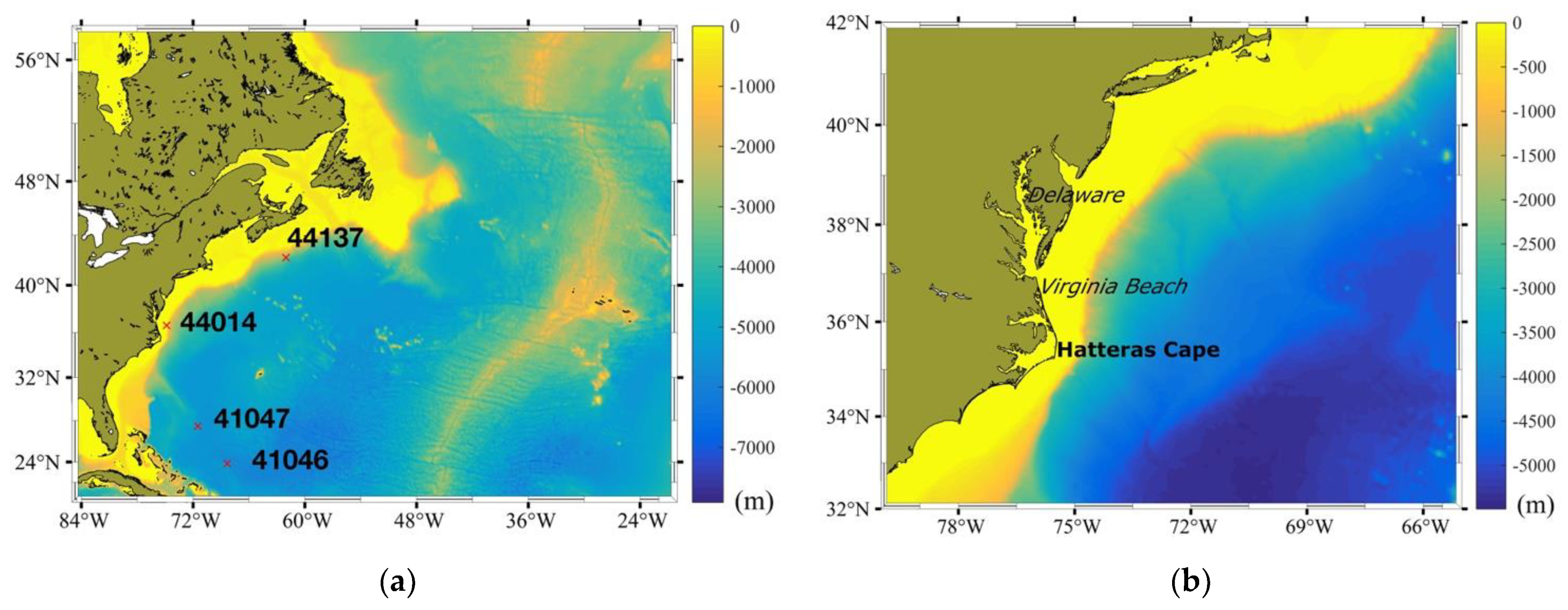
The configuration of WAM (Wave Advanced Modeling) [26,27,28] grid model covers the Gulf Stream region. In this configuration two different grids are implemented: a coarse and a nested high-resolution grid, at spatial resolution of 0.125° and 0.05°, respectively. Bathymetry grids for all domains are constructed from Etopo1 [29] from the NOAA’s National Geophysical Data Centre, with a resolution of 1 min of degree in latitude and longitude, which was linearly interpolated to the model grid. Figure 1 shows the bathymetry grids and the distribution of the WAM output locations that coincide with the wave buoys.
The wave spectrum for the coarse grid configuration is provided for 36 directional bands measured clockwise with respect to the true north, and 38 frequencies logarithmically spaced from the minimum frequency of 0.030 Hz at intervals of Df/f = 0.1. On the case of the high-resolution nested grid encompassing the Gulf Stream, 38 frequencies and 48 directions are used.
The open boundaries for the coarse grid model are forced by wave spectra taken from the ECMWF (European Centre for Medium-Range Weather Forecasts) ERA5 (ECMWF Reanalysis) reanalysis wave model (IFS documentation 2019). For the coarse and the nested grids shown in Figure 1, the ERA-5 ECMWF wind reanalysis [30] was chosen. More details about the wave model implementation used can be found in Table 1.
Current effects are considered in the WAM model (see Equation (1)). However, there are some difficulties to represent properly all the complex processes that are related with the wave–current interactions in the presence of strong currents such as Agulhas or Gulf Stream [31]. The most dramatic effects may be found when the waves propagate against the current. For sufficiently large current, wave propagation is prevented, and wave reflection occurs [32].
The evolution of the two-dimensional ocean wave spectrum F (f—frequency, θ—mean wave propagation direction, φ—latitude, λ—longitude) with respect to the frequency and direction as a function of latitude and longitude is governed by the transport Equation (1). The model is formulated in finite differences on regular and rectangular grids. In the presence of currents, the governing equation can be written as
where u is the current velocity, Cg is the group velocity, t is the time and Stot is the source function which considers all the physical processes that allow the growth and the decay of waves: the wave energy generation, dissipation, and nonlinear wave–wave interaction. The processes included in the model are wave generation by wind [33], nonlinear resonant wave–wave interactions ([34], and the whitecapping [35]).
Two independent numerical simulations are performed: with and without ocean currents. Current data comes from Mercator Ocean in the framework of the Copernicus Marine Environment Monitoring Service (CMEMS). The Operational Mercator global ocean analysis-forecast (phy-0010024) is an hourly product with a 1/12° of horizontal resolution [36]. Mercator Ocean monitoring and forecasting systems have been routinely operated in real time since early 2001.
2.2. Validation
The validation is performed for the significant wave height (Hs) using wave buoys data provided by NDBC (NOAA) (Figure 1) and Environment and Climate Canada. Table 2 shows some of the statistical parameters computed. The validation is made for the two hindcasts performed: (1) considering only waves (WWav) and (2) including currents (WCur). The bias is defined as the difference between the mean observation and the mean prediction. The scatter index (S.I.) is defined as the standard deviation of the predicted data with respect to the best fit line, divided by the mean observations.
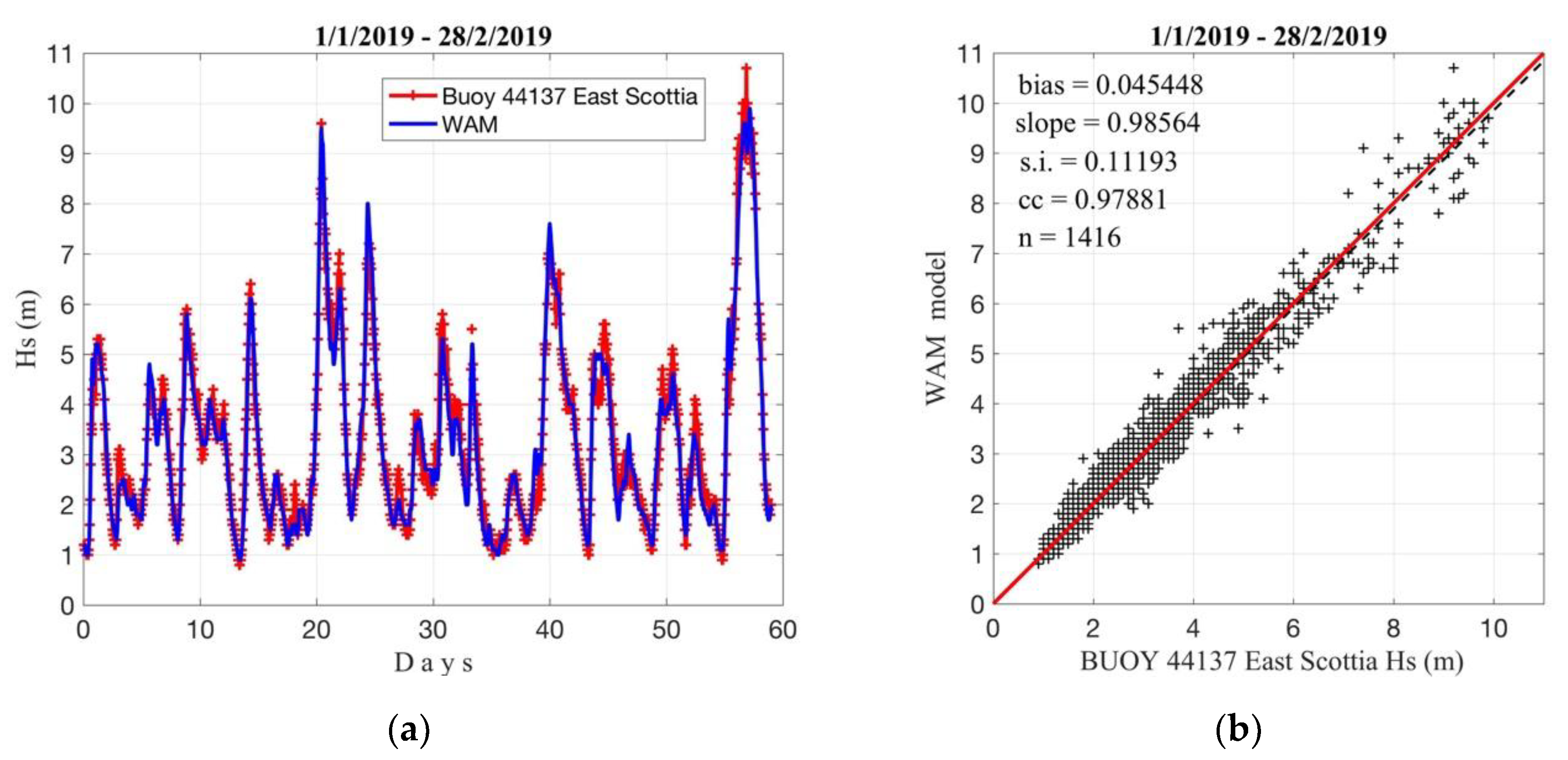
The best correlation coefficient found corresponds to the location 44137 from the simulation considering currents (0.98, case WCur with current) and the worst correlation was obtained for the wave buoy location (0.90, case WWav only waves). The scatter indexes varied in the range of 0.11 (WWav and WCur) to 0.13 (location 44137, WWav), whereas the bias varied from 0.05 (44137, WCur) and 0.13 (loc 41046, WWav). The best slope corresponded to the simulation with currents and to the location 44137 (0.99) (Table 2, Figure 2). As can be seen, the systematic deviation (bias) is always lower for the case with currents compared without currents, the absolute errors, as measured by the RMS error is lower for the simulation with currents, which also improves the dispersion (S.I) and the correlation coefficient between the hindcast and the wave buoys measurements.
The comparison of the modelled and observed Hs is depicted in Figure 2a for the best correlated simulation (considering current). As can be seen a good correlation was obtained for the location #44137 (East Scotia). During the study period at least eight storms can be identified with values higher than 5 m. The biggest storm with Hs = 11 m was underestimated by the model. In general, the model had the tendency of underestimate the observations with a positive bias (0.04) (Figure 2b, see Table 2).
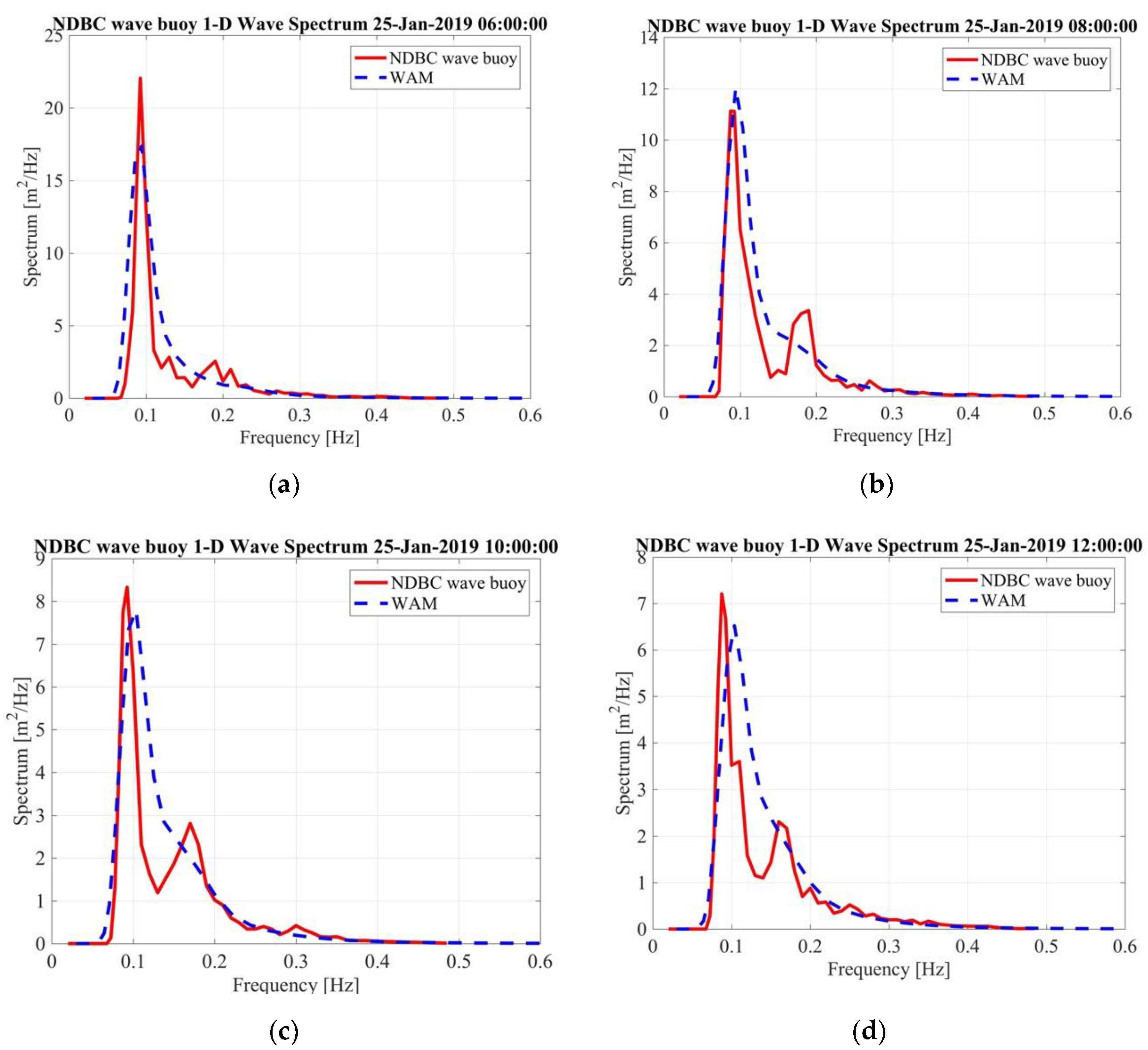
Usually, the validation of the numerical simulations is performed by a simple comparison of the typical averaged parameters (Hs, mean wave direction), but very seldom a comparison of the wave spectra is given. In terms of the spectral density in this study, a comparison (from the simulation with currents) of the one-dimensional wave spectra is presented for the location #44014 where 1d wave spectra were measured during the storm of the 25/01/2019 (Figure 3). This comparison shows that in general the wave model matches the peak frequency, and the wave spectra are of the same order of magnitude, however, sometimes the modelled spectral peak is slightly shifted to high frequencies (at 08 UTC (Coordinated Universal Time), 10 UTC, and at 12 UTC).
In this case, the wave model has less frequencies (38) and covers a higher frequency range (0.03–1.02 Hz) than the wave buoys (47 frequencies, from 0.02 Hz to 0.49 Hz). We believe it is for this reason that the differences in the spectral shapes exist. In the case of the missed second spectral peak, the model does not have sufficient resolution to capture it and/or the high frequency part components corresponding to local winds are not reproduced totally in the Era-5 reanalysis wind fields.
In addition, the measured wave spectra at times 06, 10, and 12 UTC are underestimated by the wave model whereas at high frequencies the observed wave spectra show secondary spectral peaks that the wave model cannot reproduce, which could be associated with several and different sources of errors of the numerical simulations: errors in the wind field, errors in the physical processes represented in the WAM model to cope with the wave–current interactions, some of these are: refraction by the current, reflection (absent) and wave blocking. The last one, is where waves and currents oppose each other and stop wave propagation, but the mechanism by which wave energy is removed at the blocking point is not understood yet [37].
3. Results and Discussions
Comparison of the Spatial Patterns in the Simulations with and without Currents
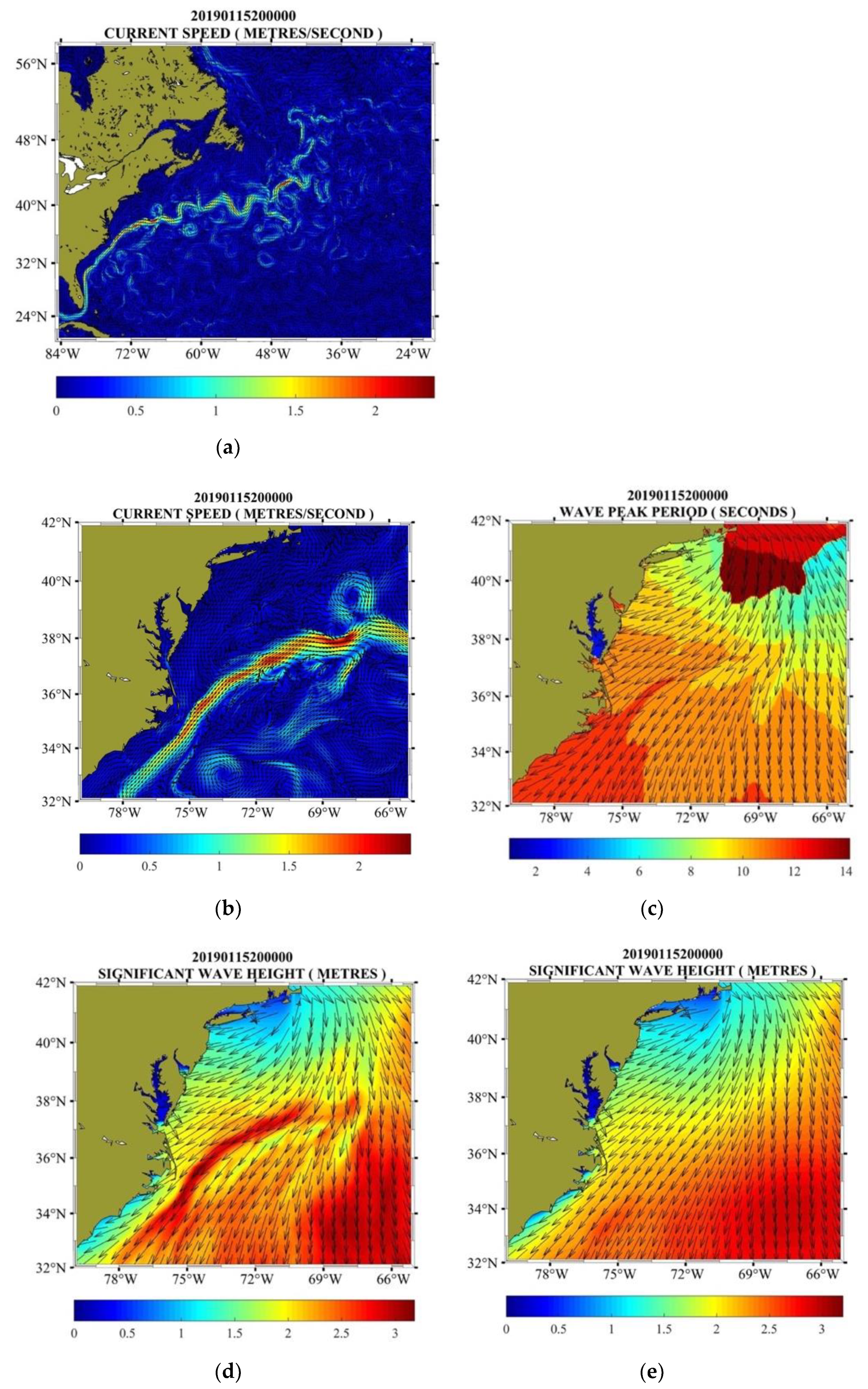
The MERCATOR current field for the coarse grid can be seen (Figure 4a) for the 15/01/2019 at 20 UTC showing current speeds higher than 2 m/s and depicting clearly the meandering character of the Gulf Stream propagating from the SW to the NE. Figure 4b shows the Gulf Stream in the frame of the high-resolution nested grid showing with more details the Gulf Stream and the meanders as obtained from the MERCATOR ocean current data.
The peak period (Figure 4c) is depicted for the same date showing high values above 12 s coinciding with the Gulf Stream from the SW side of the grid up to the latitude 36° N and the intrusion of the swell of 14 s propagating from the NE into the region of the simulation. A comparison between the modelled Hs is depicted in the bottom panels of Figure 4 from which the clear effect that has the Gulf Stream in the wave field can be seen.
Once the wave field propagates from the NE in an opposite direction facing the Gulf Stream one of the effects is the increase of the Hs inside the current (bottom left) as obtained from the simulation considering the current. In this case for the 15 January 2019 at 20 UTC the Hs reached the 3 m and repeats the shape of the Gulf Stream itself. The fact that waves propagate in opposite direction to the current increases the Hs. In addition, it seems that there are not noticeable variations in the mean wave propagation directions from both compared simulations with/without current.
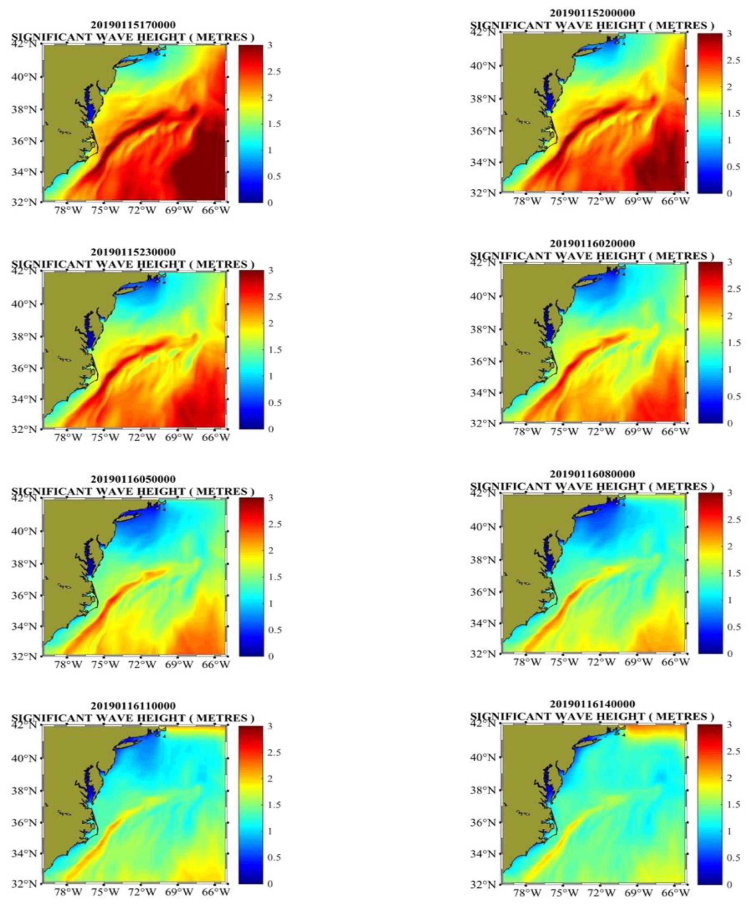
From the evolution of the wave field (15 January 2019–16 January 2019) (Figure 5) from the simulation considering currents, can be seen (top panels) the coexistent of mixed wave fields of Hs of 3 m covering almost whole the domain together with the high values of the Hs just in the location of the Gulf Stream as a fine feather which vanishes with time as the Hs decreases down to two meters on the 16 January 2019 (bottom panels).
4. Assessment of the Influence of the Gulf Stream on Waves
4.1. Analysis of Wave Spectra Along the Main Axis of the Gulf Stream
Since the interest is in knowing what the effect of the Gulf Stream on the spectral shapes is, the objective is to analyze the modelled wave spectra on the current. In this regard, hundreds of wave spectra were analyzed along the current axis. The Gulf stream’s axis is found by looking for the grid nodes with the maximum current magnitude at each grid longitude.
Two main cases are analyzed: when waves and the current are opposed and when waves and the current propagate with the almost same direction.
4.1.1. Case #1: Waves and Current Opposed
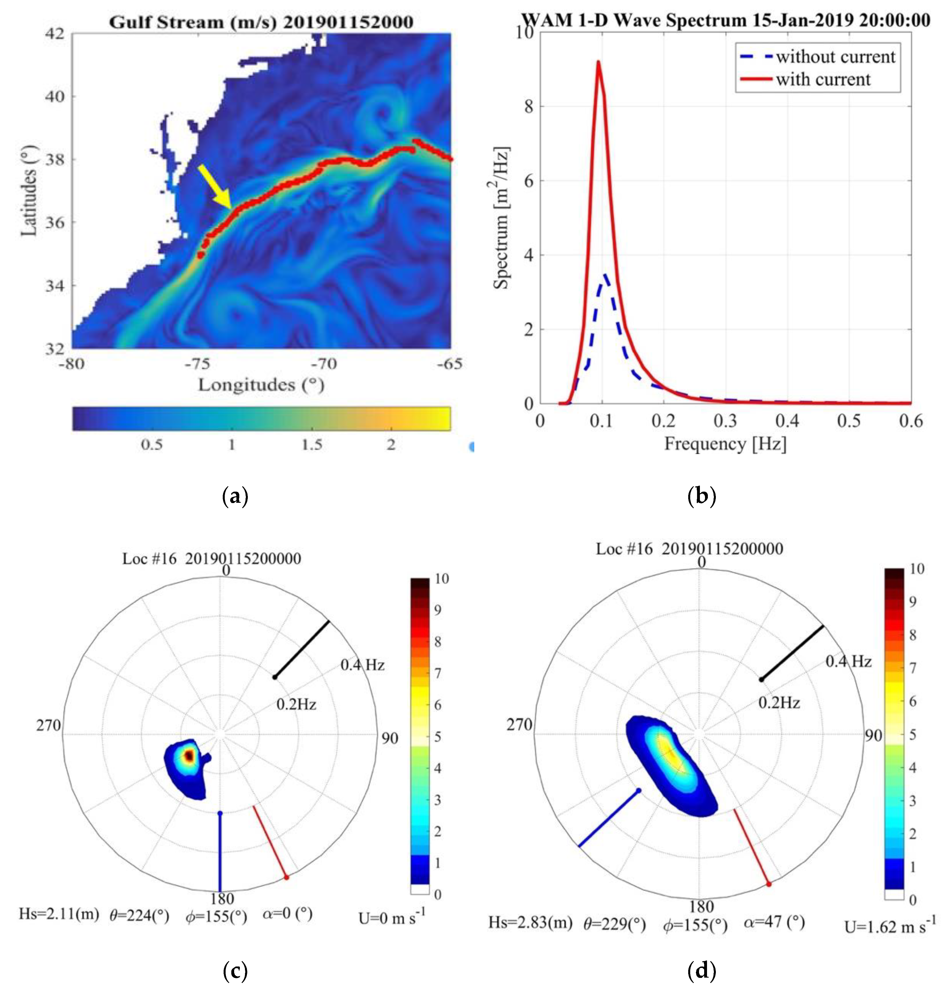
A comparison of the wave spectra from simulations with and without currents for the dates 15 January 2019 at 20 UTC is shown in Figure 6 at location #16 (Figure 6a). As can be seen the Gulf Stream flows almost stationary from the SW to NE (Figure 4a), at the same time waves propagates to the SW (Figure 4d) contrary to the current. This natural condition result in certain spectral shapes.
The effect of the Gulf Stream on the spectral wave shape is clear (Figure 6). For the 1d spectrum (Figure 6b), the blocking of wave energy due to the opposing current causes an increase in the spectral peak energy and in the Hs. The 2D spectrum without currents (Figure 6c) shows higher local energy levels with peak spectral energy above 10 m2/Hz/radian and is limited in the 210°–270° sector; however, the total spectral energy as measured by the Hs is lower (2.11 m) than the case with currents (2.83 m; Figure 6d). In this case, while the peak energy is lower, the spectrum is wider, occupying the whole SW sector with high energy levels spread instead of concentrated in the spectral peak region. The effect of the current on the 2D wave spectrum is thus to spread the wave energy due to the refraction caused by the current’s spatial gradients.
4.1.2. Case #2. Waves and Current Almost Aligned Propagating to the NE
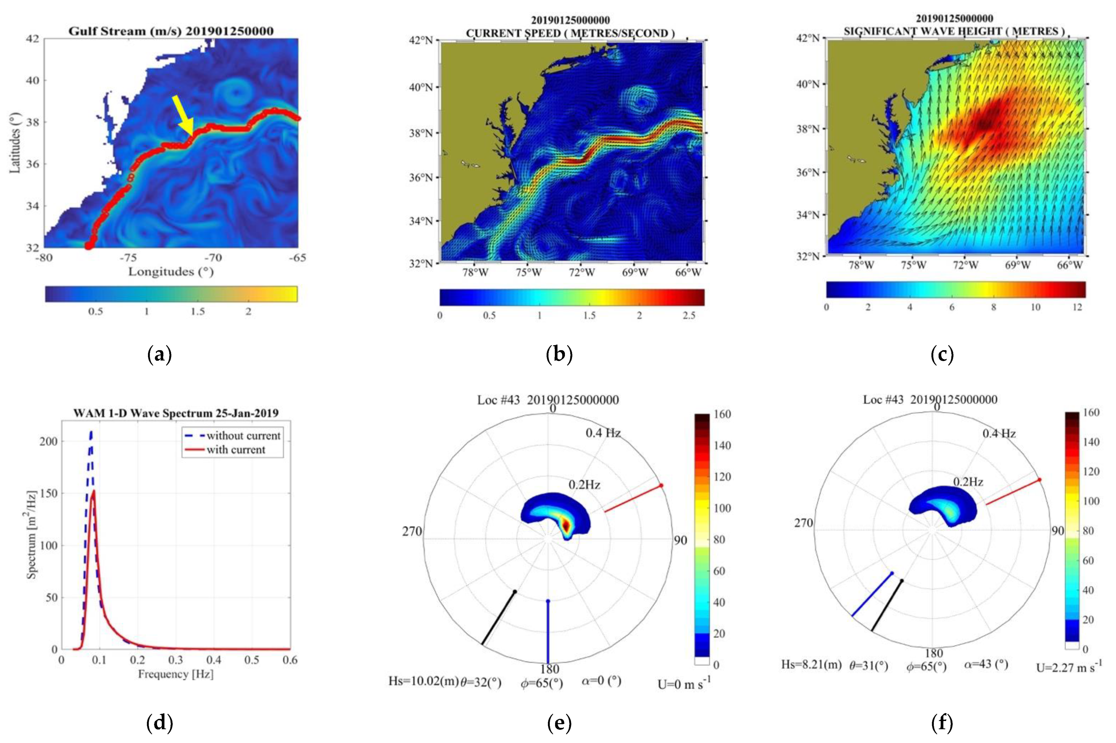
In the case when waves are almost aligned with the current (from the SW quadrant) and the wind blows from the NE (see the red vector in the wave spectra) the spectral wave energy is higher as can be seen in the comparison of the directional wave spectra of Figure 7e,f. Large swells coming from the SW are due to the formation of extra-tropical cyclones in the Gulf Stream region, which propagate north-easterly along the US Atlantic coast [38].
Again, the simulation with currents is observed to produce broader wave spectra, but since the waves are propagating in the same direction of the current the Hs decreases almost 2 m (Hs = 10.02 m without currents and Hs = 8.20 m with current) Figure 7e,f.
4.2. Analysis of the Characteristic Parameters Along a Transect Crossing the Gulf Stream
This section focuses on the analysis of the Hs and mean wave direction obtained from simulations with and without currents along a transversal transect. The transect was chosen in such a way that it crosses the Gulf Stream along the 75° W meridian between the latitude 33° N and 36° N and the analysis is performed from the South to the North. The objective was to understand how the velocity gradient affects the Hs.
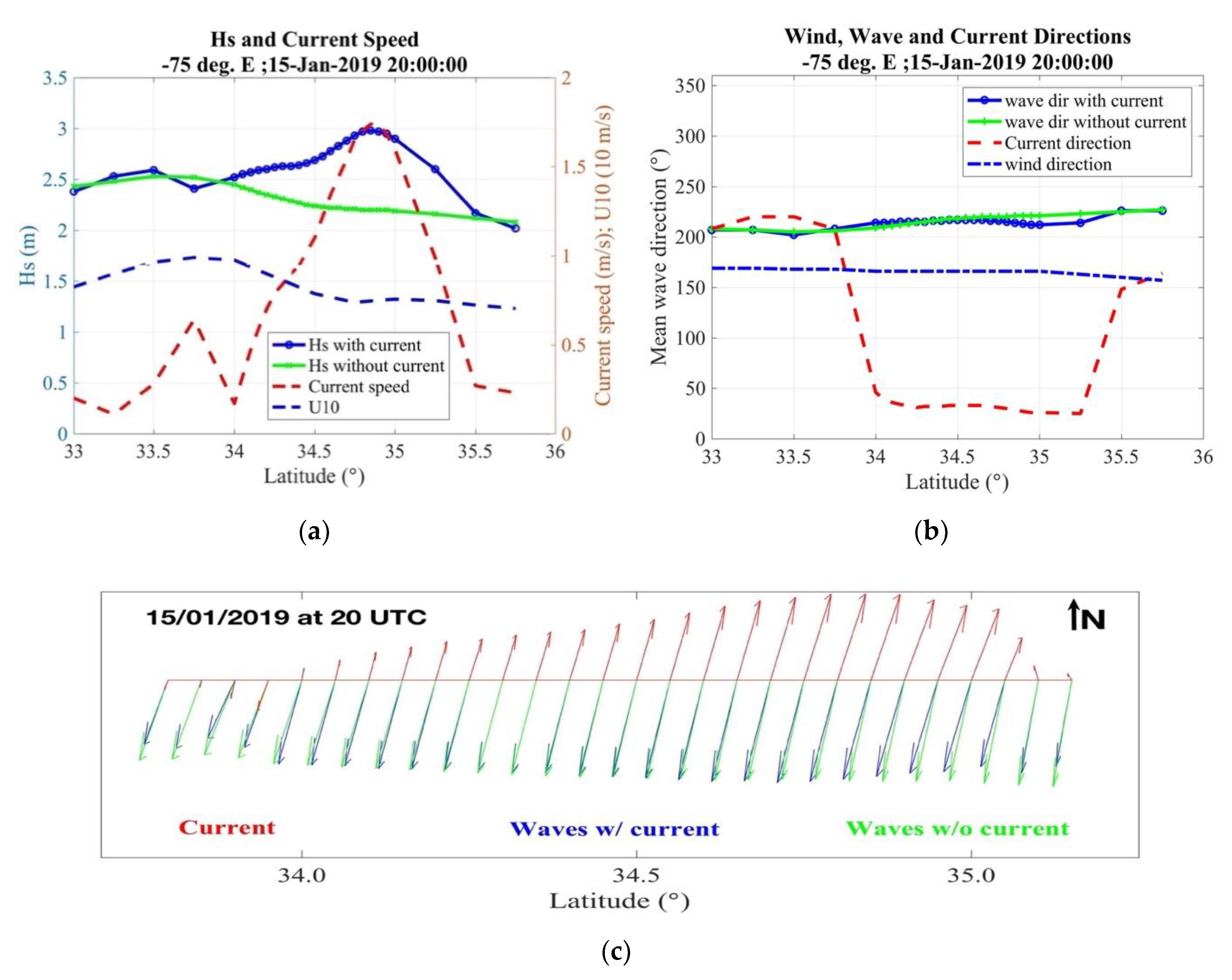
It can be seen how the Hs increases along the transect that crosses the Gulf Stream. The Hs is correlated with the current speed (max 1.75 m/s, see the right Y axis red dashed line), and its maximum value (Figure 8a, blue line with circles (with current)) is observed in the centre of the Gulf Stream between the 34.5° N and 35° N. In addition, the wind speed is about 7.5 m/s, which does not favour the increase of waves.
The Hs increases with the current speed only in the case that has currents, and it is conditioned by the orientation of the waves with respect to the Gulf Stream (see directions in the right panel), from latitude 34° N up to latitude 35.25° N. It is noteworthy that in this case the current does no change appreciably the wave propagation direction (Figure 8c).
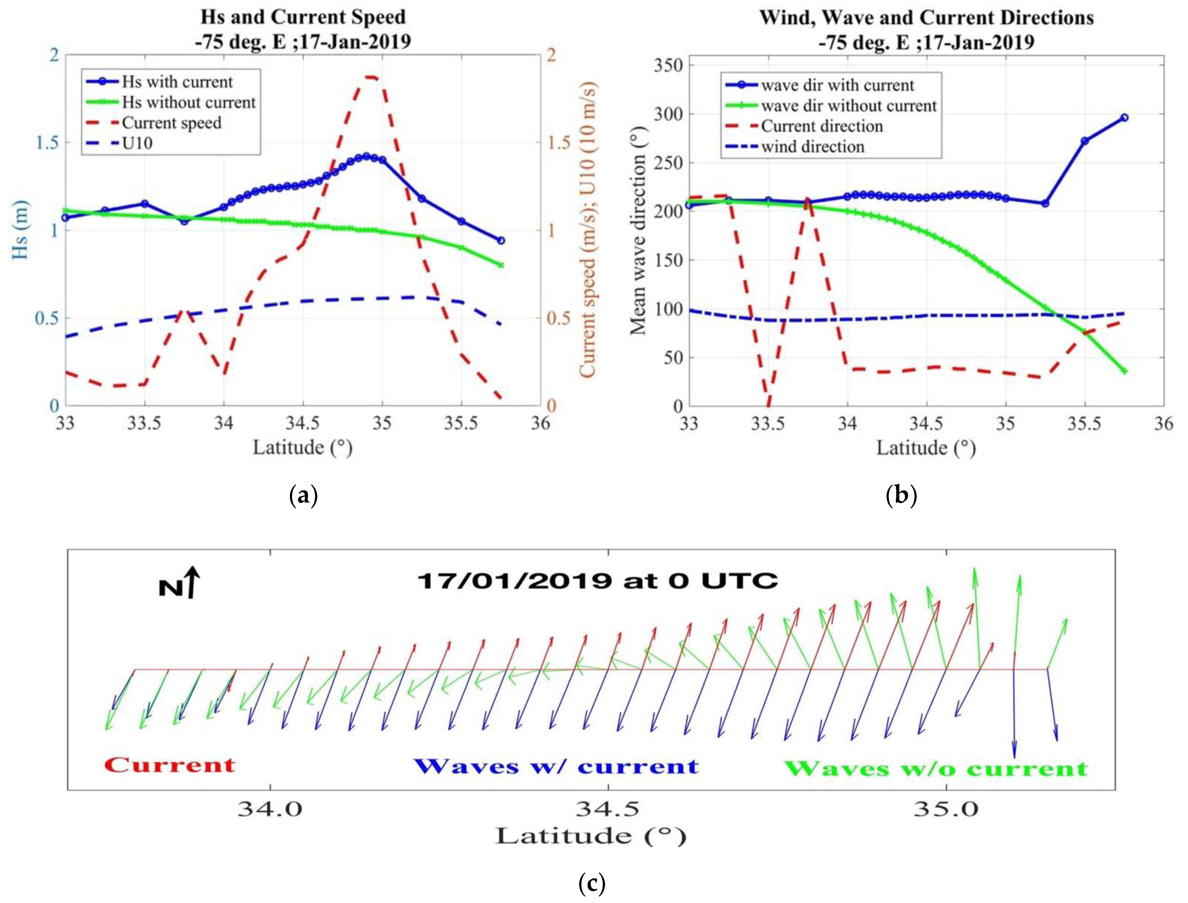
In the case that waves are opposed to the Gulf Stream (see the green, the blue and the dashed red lines, Figure 9a), it was observed from the simulation with current the same behavior as in Figure 8, i.e., the Hs increases (blue line with circles) in the centre between the latitudes 34.5° N and 35° N of the Gulf Stream (Figure 9a). Here the wind speed is about 5 m/s blowing from the NW, so the Hs does grow noticeably (Hs = 1.48 m). On the contrary the Hs (simulation without current, green line, left panel) does not show this increase of the Hs, on the contrary, it decreases with distance along the meridian 75° W. However, the most noticeable effect is in the wave propagation direction due to the current (Figure 9c). It can be observed that without currents, the direction changes from SW at 34° N to almost N at 35° N, while for the simulation with currents, the propagation direction is constant along the transect.
As shown, in general, the Gulf Stream speed varies from the high-speed centre of the current to the lower speed away from the centre. It seems that due to the non-uniform speed distribution across the Gulf Stream the focusing takes places generating steep waves, when wind flows from the North (Figure 8 and Figure 9), so the wave energy is focused in the centre of the stream. With a northerly wind the focusing takes place, which concentrate the wave energy in the centre of the stream that may lead to dangerous seas.
On the contrary when the wind flows from South the defocusing of the wave energy takes place resulting in milder waves.
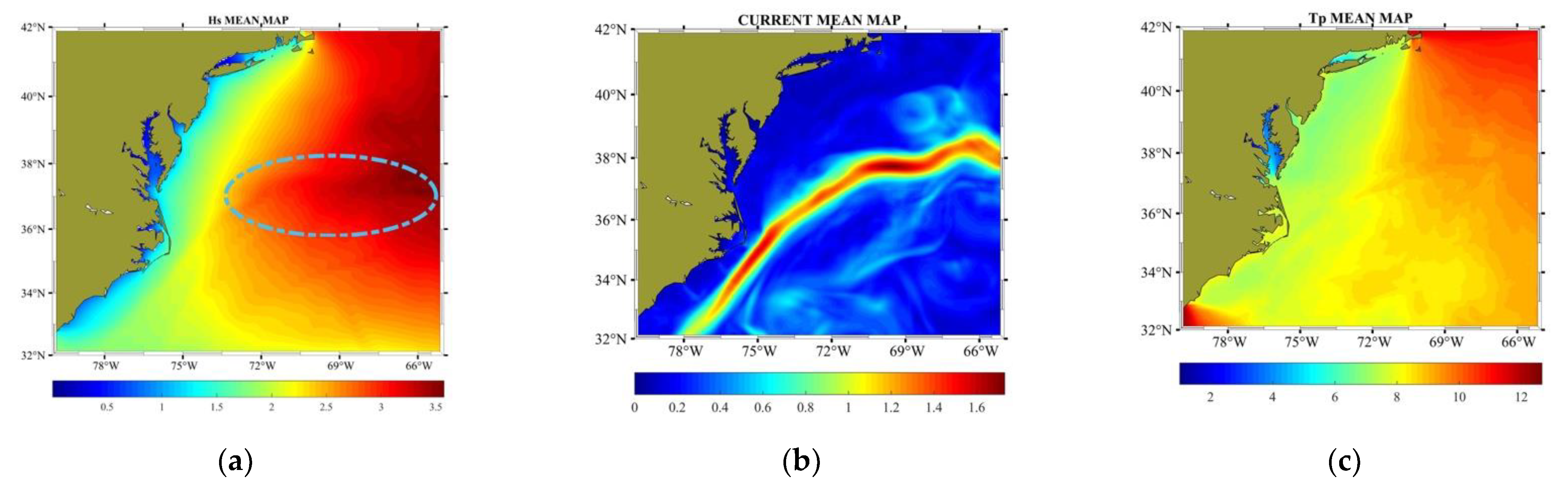
Some recommendations can be made regarding the navigation in the region of the Gulf Stream. From the hourly mean maps of the Hs, Tp, and the surface current it can be seen that dangerous places for the navigation are located along the path of the Gulf Stream showing high mean values of Tp (8–10 s) that coincides with the current, as well as the high Hs mean values ranging from 3 to 3.5 m. The most dangerous area for the navigation is located between the 36° N and 38° N and between the 73° W and 65° W (Figure 10a). This recommendation must be taken with caution since the performed simulations are short. In the future higher resolution simulations not only in time and space but also in the wave spectrum are planned.
The above results are in line with the reported ship accidents in severe weather in [39], where the region of the Gulf Stream was identified as one of the most frequent for accidents due to higher wave heights for a given wave period.
5. Conclusions
A characterization of inhomogeneities of the ocean surface wave field in the Gulf Stream region has been presented where strong influence of current on waves take place. This was accomplished with numerical simulations using a third-generation wave model with and without current.
In general, it was observed that the Hs is higher in the centre of the Gulf Stream than in the periphery. This fact has implications for the navigation.
With a northerly wind situation, focusing takes place, concentrating the wave energy in the centre of the Gulf Stream that may lead to dangerous seas. On the contrary when the wind flows from South the defocusing takes place resulting in milder waves. This conclusion is important to be taken into account for the shipping industry.
The wave spectrum has an elongated shape and steep peak when wave and current are opposed. The effect of the Gulf Stream resulted in a resulted in a widening of the spectrum angular distribution.
The limitations of the present study lies on three main items: the current field at 9 km of spatial resolution does not reproduce well the eddies, the bathymetry data also could have a higher resolution than the used (Etopo1), and the spatial resolution of the wave model need to be increased as well to fully characterize the influence of the Gulf Stream on the wave characteristics. In a follow-up study these three items will be considered.
Author Contributions
S.P.d.L.: Conceptualization; methodology; validation; formal analysis; writing—original; C.G.S.: writing—review and editing. All authors have read and agreed to the published version of the manuscript.
Funding
This work contributes to the Strategic Research Plan of the Centre for Marine Technology and Ocean Engineering (CENTEC), which is financed by the Portuguese Foundation for Science and Technology (Fundação para a Ciência e Tecnologia—FCT) under contract UIDB/UIDP/00134/2020.
Data Availability Statement
Data is available from the authors upon reasonable request.
Conflicts of Interest
The authors declare no conflict of interest.
References
- Stommel, H. The westward intensification of wind-Driven ocean currents. Trans. Am. Geophys. Union 1984, 29, 202–206. [Google Scholar] [CrossRef]
- Pedlosky, J. Ocean Circulation Theory, 1st ed.; Springer: Berlin/Heidelberg, Germany, 1996; p. 456. [Google Scholar] [CrossRef]
- Lutjeharms, J.R.E. The Agulhas Current; Springer: Berlin/Heidelberg, Germany, 2006; ISBN 10 3-540-42392-3. Available online: https://link.springer.com/content/pdf/10.1007/3-540-37212-1.pdf (accessed on 30 September 2020).
- Gula, J.; Molemaker, J.; McWilliams, J. Gulf Stream dynamics along the south eastern U.S. seaboard. J. Phys. Oceanogr. 2015, 45, 690–715. [Google Scholar] [CrossRef]
- Marez, C.D.; Lahaye, N.J.; Gula, J. Interaction of the Gulf Stream with small scale topography: A focus on lee waves. Sci. Rep. 2020, 10, 1–10. [Google Scholar] [CrossRef] [PubMed] [Green Version]
- Glenn, S.M.; Ebbesmeyer, C. The structure and propagation of a Gulf Stream frontal eddy along the North Carolina shelf break. J. Geophys. Res. 1994, 99, 5029–5046. [Google Scholar] [CrossRef]
- Thomas, G.P. Wave-Current Interactions: An Experimental and Numerical Study. Part 1. Linear Waves. J. Fluid Mech. 1981, 110, 457–474. [Google Scholar] [CrossRef]
- Kemp, P.H.; Simons, R.R. The Interaction between Waves and a Turbulent Current: Waves Propagating with the Current. J. Fluid Mech. 1982, 116, 227–250. [Google Scholar] [CrossRef] [Green Version]
- Kemp, P.H.; Simons, R.R. The Interaction of Waves and a Turbulent Current: Waves Propagating against the Current. J. Fluid Mech. 1983, 130, 73–89. [Google Scholar] [CrossRef] [Green Version]
- Nwogu, O.G. Effect of Steady Currents on Directional Wave Spectra. In Proc.12th Int. Conf. On Offshore Mechanics and Arctic Engineering (OMAE); OMAE: Glasgow, Scotland, 1993; Volume 1, pp. 25–32. [Google Scholar]
- Guedes Soares, C.; Pablo, H.D. Experimental study of the transformation of wave spectra by a uniform current. Ocean Eng. 2006, 33, 293–310. [Google Scholar] [CrossRef]
- Onorato, M.; Proment, D.; Toffoli, A. Triggering rogue waves in opposing currents. Phys. Rev. Lett. 2011, 107, 184502. [Google Scholar] [CrossRef]
- Toffoli, A.; Waseda, T.; Houtani, H.; Cavaleri, L.; Onorato, M. Rogue waves in opposing currents: An experimental study on deterministic and stochastic wave trains. J. Fluid Mech. 2015, 769, 277–297. [Google Scholar] [CrossRef] [Green Version]
- Melville, W.; Romero, L.; Kleiss, J. Extreme wave events in the Gulf of Tehuantepec. In Proceedings of the Rogue Waves: 14th ‘Aha Huliko‘a Hawaiian Winter Workshop 2005, University of Hawai‘i at Manoa, Honolulu, HI, USA, 23–28 January 2005. [Google Scholar]
- Romero, L.; Lenain, L.; Melville, W.K. Observations of surface wave-Current interaction. J. Phys. Oceanogr. 2017, 47, 615–632. [Google Scholar] [CrossRef]
- Rusu, L.; Guedes Soares, C. Modelling the Wave-Current Interactions in an Offshore Basin using the SWAN Model. Ocean Eng. 2011, 38, 63–76. [Google Scholar] [CrossRef]
- Booij, N.; Ris, R.C.; Holthuijsen, L.H. A third-Generation wave model for coastal regions. Part 1: Model description and validation. J. Geophys. Res. 1999, 104, 7649–7666. [Google Scholar] [CrossRef] [Green Version]
- Rusu, L.; Bernardino, M.; Guedes Soares, C. Modelling the influence of currents on wave propagation at the entrance of the Tagus estuary. Ocean Eng. 2011, 38, 1174–1183. [Google Scholar] [CrossRef]
- Hayes, J.G. Ocean current wave interaction study. J. Geophys. Res. 1980, 85, 5025–5031. [Google Scholar] [CrossRef]
- Mathiesen, M. Wave refraction by a current whirl. J. Geophys. Res. 1987, 92, 3905–3912. [Google Scholar] [CrossRef]
- Holthuijsen, L.H.; Tolman, H.L. Effects of the Gulf Stream on ocean waves. J. Geophys. Res. 1991, 96, 12755–12771. [Google Scholar] [CrossRef]
- Restano, M.; Esa-Esrin, S.C.; Passaro, M.; Vignudelli, S.; Benveniste, J.; Tum, C.; Esrin, E. Wave-Current interactions in the Agulhas Current. In Proceedings of the 12th Coastal Altimetry Workshop (CAW12), ESA-ESRIN, Fraskati (Rome), Italy, 4–7 February 2020; p. 39. [Google Scholar]
- Ponce de León, S.; Guedes Soares, C.; Johannessen, J.A. Modelling of the Stokes Drift in the Agulhas Current System; Guedes Soares, C., Santos, T.A., Eds.; Developments in Maritime Technology and Engineering: London, UK, 2021. [Google Scholar]
- Wang, D.W.; Liu, A.K.; Peng, C.Y.; Meindl, E.A. Wave-Current interaction near the Gulf Stream during the Surface Wave Dynamics Experiment. J. Geophys. Res. 1994, 99, 5065–5079. [Google Scholar] [CrossRef]
- Ardhuin, F.; Gille, S.T.; Menemenlis, D.; Rocha, C.B.; Rascle, N.; Chapron, B.; Gula, J.; Molemaker, J. Small-Scale open-Ocean currents have large effects on wind-Wave heights. J. Geophys. Res. Oceans 2017, 122, 4500–4517. [Google Scholar] [CrossRef] [Green Version]
- WAMDI Group. The WAM Model—A Third Generation Ocean Wave Prediction Model. J. Phys. Oceanogr. 1988, 18, 1775–1810. [Google Scholar] [CrossRef] [Green Version]
- Komen, G.J.; Cavaleri, L.; Donelan, M.A.; Hasselmann, K.; Hasselmann, S.; Janssen, P.A.E.M. Dynamics and Modelling of Ocean Waves; Cambridge University Press: Cambridge, UK, 1994. [Google Scholar]
- Gunther, H.; Berenhs, A. The WAM Model, Validation Document, Version 454; GKSS: Hamburg, Germany, 2012; p. 92. [Google Scholar]
- Amante, C.; Eakins, B.W. ETOPO1 1 Arc-Minute Global Relief Model: Procedures, Data Sources and Analysis. In NOAA Technical Memorandum 2009; NESDIS NGDC-24; National Geophysical Data Center, NOAA: Boulder, CO, USA, 2009. [Google Scholar] [CrossRef]
- Hersbach, H.; Bell, W.; Berrisford, P.; Horányi, A.; Muñoz-Sabater, J.; Nicolas, J.; Radu, R.; Schepers, D.; Simmons, A.; Soci, C.; et al. Global reanalysis: Goodbye ERA-Interim, hello ERA5. Chapter Meteorol. 2019, 59, 17–24. [Google Scholar] [CrossRef]
- Ponce de León, S.; Guedes Soares, C. Influence of Agulhas Current Retroflection on Extreme and Abnormal Waves. Unpublished work. 2020. [Google Scholar]
- IFS Documentation-Cy46r1. Operational Implementation. Part VII: ECMWF Wave Model. 99 pp. Copyright 2019 European Centre for Medium-Range Weather Forecasts Shinfield Park, Reading, RG2 9AX, England. Available online: https://www.ecmwf.int/sites/default/files/elibrary/2019/Part-VII-ECMWF-Wave-Model.pdf (accessed on 6 June 2019).
- Janssen, P.A.E.M. Quasi-Linear theory of wind wave generation applied to wave forecasting. J. Phys. Oceanogr. 1991, 21, 1631–1642. [Google Scholar] [CrossRef] [Green Version]
- Hasselmann, S.; Hasselmann, K.; Allender, J.H.; Barnett, T.P. Computations and parameterizations of the nonlinear energy transfer in a gravity-Wave spectrum, Part II. J. Phys. Oceanogr. 1985, 15, 1378–1391. [Google Scholar] [CrossRef] [Green Version]
- Komen, G.J.; Hasselmann, S.; Hasselmann, K. On the existence of a fully developed wind-Sea spectrum. J. Phys. Oceanogr. 1984, 14, 1271–1285. [Google Scholar] [CrossRef]
- Lellouche, J.-M.; Greiner, E.; Galloudec, L.O.; Garric, G.; Regnier, C.; Drevillon, M.; Benkiran, M.; Testut, C.-E.; Bourdalle-Badie, R.; Gasparin, F.; et al. Recent updates to the Copernicus Marine Service global ocean monitoring and forecasting real-Time 1/12°high-resolution system. Ocean. Sci. 2018, 14, 1093–1126. [Google Scholar] [CrossRef] [Green Version]
- Alves, J.-H.; Ardhuin, A.; Babanin, M.; Banner, A.; Benner, M.; Belibassakis, K.A.; Benoit, M.; Groeneweg, J.; Herbers, T.H.C.; Hwang, P.; et al. Wave modelling—The state of the art. Prog. Oceanogr. 2007, 75, 603–674. [Google Scholar]
- Ponce de León, S.; Bettencourt, J.H. Composite analysis of North Atlantic extra-Tropical cyclone waves from satellite altimetry observations. Adv. Space Res. 2019. [Google Scholar] [CrossRef]
- Guedes Soares, C.; Bitner-Gregersen, E.M.; Antao, P. Analysis of the frequency of ship accidents under severe North Atlantic weather conditions. In Proceedings of the Design and Operation for Abnormal Conditions II, RINA, London, UK, 6–7 November 2001; pp. 221–230. [Google Scholar]
Figure 1.
Bathymetry grids: coarse (a) and nested (b); locations of the NDBC wave buoys and WAM outputs.
Figure 1.
Bathymetry grids: coarse (a) and nested (b); locations of the NDBC wave buoys and WAM outputs.

Figure 2.
Comparison of the Hs time series for the wave buoy #44137 (a) from the simulation considering currents (blue line) and from the wave buoys observations (red line) and the scatter plots (b).
Figure 2.
Comparison of the Hs time series for the wave buoy #44137 (a) from the simulation considering currents (blue line) and from the wave buoys observations (red line) and the scatter plots (b).

Figure 3.
Comparison of the 1D wave spectra for the location of the NDBC wave buoy #44014 (Virginia from the simulation considering currents (blue line) and from the wave buoy observations (red line) for the 25 of January 2019 for 06 UTC (a), 08 UTC (b), 10 UTC (c) and12 UTC (d). Latitude: 36.609° N, Longitude: 74.842° W.

Figure 4.
Current velocity field (source: MERCATOR ocean) from the coarse grid domain (a), the current field from the high resolution nested grid (b), the WAM peak period (c), WAM modelled Hs considering currents (d) and the WAM Hs without current (e) for the 15th of January 2019 at 20 UTC.
Figure 4.
Current velocity field (source: MERCATOR ocean) from the coarse grid domain (a), the current field from the high resolution nested grid (b), the WAM peak period (c), WAM modelled Hs considering currents (d) and the WAM Hs without current (e) for the 15th of January 2019 at 20 UTC.

Figure 5.
Evolution of the wave field. Row wise from the top from the 15 January 2019 at 17 UTC up to 16/01/2019 at 14 UTC.
Figure 5.
Evolution of the wave field. Row wise from the top from the 15 January 2019 at 17 UTC up to 16/01/2019 at 14 UTC.

Figure 6.
The Gulf Stream snapshot (a) showing the position of the wave spectra along the current, comparison of the 1D WAM wave spectra (b). The 2D WAM total wave spectrum from the simulation without currents (c) and from the simulation considering the current (d) for the date 15 January 2019 at 20 UTC. Lat.: 36.17° N, 73.67° W. Red arrow-wind direction, black arrow-mean wave propagation direction, blue arrow-current direction. Symbols in the bottom of each wave spectra: φ (wind direction), θ (wave direction), α (current direction), U (Current velocity). Wave and current direction arrows were rotated 180° to show following or opposing waves and current. The arrowhead (circle) points to where the waves and currents propagate (oceanographic convention).

Figure 7.
The Gulf Stream snapshot (a) showing the position of the wave spectra along the current, current with vectors (b), wave field (c). Comparison of the 1D WAM wave spectra (d), the 2D WAM total wave spectrum (e) from the simulation without currents and considering the current (f) for the date 25 January 2019 at 00 UTC at location #43. Lat.: 37.167° N, 71.417° W. Red arrow-wind direction, black arrow-mean wave propagation direction, blue arrow-current direction.

Figure 8.
The Hs and the current speed (a) and the mean wave propagation direction and the current direction (b) along latitudes cross section from 33° up to 36° N from the South to the North keeping the same longitude −75° West. Feather plot showing the vectors (c).
Figure 8.
The Hs and the current speed (a) and the mean wave propagation direction and the current direction (b) along latitudes cross section from 33° up to 36° N from the South to the North keeping the same longitude −75° West. Feather plot showing the vectors (c).

Figure 9.
The Hs, wind speed (U10) and the current speed (a); the mean wind/wave propagation direction and the current direction (b) along latitudes cross section from 33° up to 36° N from the South to the North keeping the same longitude −75° West. Feather plot showing the vectors (c).
Figure 9.
The Hs, wind speed (U10) and the current speed (a); the mean wind/wave propagation direction and the current direction (b) along latitudes cross section from 33° up to 36° N from the South to the North keeping the same longitude −75° West. Feather plot showing the vectors (c).

Figure 10.
The averaged maps over the simulation winter period of 2019 for the Hs (a) and the dangerous places for the navigation (cyan dashed ellipse), the surface current (b) and the peak period map (c).
Figure 10.
The averaged maps over the simulation winter period of 2019 for the Hs (a) and the dangerous places for the navigation (cyan dashed ellipse), the surface current (b) and the peak period map (c).


Table 1.
Parameters of the WAM model implementation for Gulf Stream.
| Parameters | Coarse Grid | Nested Grid |
|---|---|---|
| Simulation period | 01/01/2019–28/02/2019 | |
| Geographical domain | 58° N, 20° N, 20° W, 85° W | 42° N, 32° N, 65° W, 80° W |
| Spatial resolution | 0.125° | 0.05° |
| Number of points | (521, 305) 158,905 | (301, 201) 60,501 |
| Number of directional bands | 36 | 48 |
| Number of frequencies | 38 | 38 |
| Frequency range (Hz) | 0.03–1.0201 Hz | |
| Type of spectral model | Deep water | |
| Propagation | Spherical | |
| Sin + Sdis from WAM cycle 4 (ECMWF WAM) | Yes | |
| Wind input | [33] | |
| Whitecapping dissipation | [35] | |
| Nonlinear interactions | [34] | |
| Current refraction | Yes | |
| Wind input time step (hour) | 1 | |
| Wave model output time step (hour) | 1 | |
| Integration & source time steps (seconds) | 200 | 90 |
| Wind data | Era-5 reanalysis | |
| Bathymetry data | Etopo 1 | |
Table 2.
Statistics for the Hs. S.I.—Scatter Index; cc-correlation coefficient, n—number of records. Bias, the best-fit scatter index and slopes between wave buoys observations and modelled Hs from WAM. Left column-results from simulation without current (WWav); Right column-results from simulation considering wave–current interactions (WCur).
| Parameter | Location 44137 | Location 41046 | Location 41047 | |||
|---|---|---|---|---|---|---|
| Coordinates (latitude, longitude) | 42.260° N | 62° W | 23.822° N | 68.822° W | 27.514° N | 71.494° N |
| simulation | WWav | WCur | WWav | Wcur | WWav | WCur |
| bias | 0.06 | 0.04 | 0.134 | 0.095 | 0.11 | 0.08 |
| slope | 0.97 | 0.99 | 0.918 | 0.94 | 0.94 | 0.95 |
| S.I. | 0.13 | 0.11 | 0.123 | 0.123 | 0.11 | 0.11 |
| RMSE | 0.44 | 0.36 | 0.253 | 0.24 | 0.23 | 0.22 |
| cc | 0.96 | 0.98 | 0.90 | 0.91 | 0.94 | 0.95 |
| n | 1416 | 1414 | 1414 | |||
Publisher’s Note: MDPI stays neutral with regard to jurisdictional claims in published maps and institutional affiliations. |
© 2021 by the authors. Licensee MDPI, Basel, Switzerland. This article is an open access article distributed under the terms and conditions of the Creative Commons Attribution (CC BY) license (http://creativecommons.org/licenses/by/4.0/).
Share and Cite
MDPI and ACS Style
Ponce de León, S.; Guedes Soares, C. Numerical Modelling of the Effects of the Gulf Stream on the Wave Characteristics. J. Mar. Sci. Eng. 2021, 9, 42. https://doi.org/10.3390/jmse9010042
AMA Style
Ponce de León S, Guedes Soares C. Numerical Modelling of the Effects of the Gulf Stream on the Wave Characteristics. Journal of Marine Science and Engineering. 2021; 9(1):42. https://doi.org/10.3390/jmse9010042
Chicago/Turabian StylePonce de León, Sonia, and C. Guedes Soares. 2021. "Numerical Modelling of the Effects of the Gulf Stream on the Wave Characteristics" Journal of Marine Science and Engineering 9, no. 1: 42. https://doi.org/10.3390/jmse9010042
Note that from the first issue of 2016, this journal uses article numbers instead of page numbers. See further details here.